Global optimization using Lévy flights

Abstract

This paper studies a class of enhanced diffusion processes in which random walkers perform Lévy flights and apply it for global optimization. Lévy flights offer controlled balance between exploitation and exploration. We develop four optimization algorithms based on such properties. We compare new algorithms with the well-known Simulated Annealing on hard test functions and the results are very promising.

Key words: Lévy flights, global optimization.
This is an edited version of a paper originally published in Proceedings of Second National Symposium on Research, Development and Application of Information and Communication Technology (ICT.rda’04), Hanoi, Sept 24-25, 2004.

1 Introduction

Optimization can be characterized as a process to minimize an objective function over a bounded or unbounded space. Of the widely used class of optimization algorithms known as meta-heuristics, that many of them imitate natural processes such as Simulated Annealing (SA - originated in physics), Genetic Algorithm (GA - imitating the Darwinian process of natural selection) [1], Ant Colony Optimization (ACO – mimicking behavior of foraging ants) [2] and Particle Swarm Optimization (PSO – modeling the flocking and schooling by birds) [3]. In particular, SA and GA have been practically successful although they never guarantee to reach global optima within limited time.

This paper studies a group of stochastic processes frequently observed in physics and biology called Lévy flights [4][5]. The goal is to realize the claim by Gutowski that Lévy flights can be used in optimization [6]. A new class of meta-heuristic algorithms called LFO (Lévy Flights Optimization) is introduced. To our knowledge, similar work has not been introduced in the optimization literature.

The rest of paper is organized as the following. Sec. 2 outlines some fundamentals of Lévy flights. Sec. 3 introduces four new LFO algorithms. Sec. 4 reports experiments and results. The last section provides several possible outlooks.

2 Lévy flights

Extensive investigations in diffusion processes have revealed that there exist some processes not obeying Brownian motion. One class is enhanced diffusion, which has been shown to comply with Lévy flights [5]. The Lévy flights can be characterized by following probability density function:

$$P(x) \sim \left|x\right|^{-1-\beta}\,\,\mbox{as}\,\,x\rightarrow\infty,\,\,\mbox{where}$$

$$0 <\beta\leq 2$$ (1)

Note that with $\beta\leq 0$, the distribution in Eq. (1) cannot be normalized, therefore it has no physical meaning although our computation needs not be concerned about such problem. For $0<\beta<1$, the expectation does not exist.

For the interest of this paper, we consider a random walk where step length $l$ obeys the distribution:

$$P(l)=\frac{\beta}{l_{0}\left(1+\frac{l}{l_{0}}\right)^{1+\beta}}$$ (2)

This is a normalized version of [6] with the scale factor $l_{0}$ added since it is more natural to think in term of physical dimension of given space. This form preserves the property of distribution in Eq. (1) for large $l$ but it is much simpler to deal with small $l$. The distribution is heavy-tailed, as shown on Fig. 1(a).

It is not difficult to verify that $l$ can be randomly generated as follows:

$$l=l_{0}\left(\frac{1}{U^{1/\beta}}-1\right)$$ (3)

where $U$ is uniformly distributed in the interval $[0,1)$.

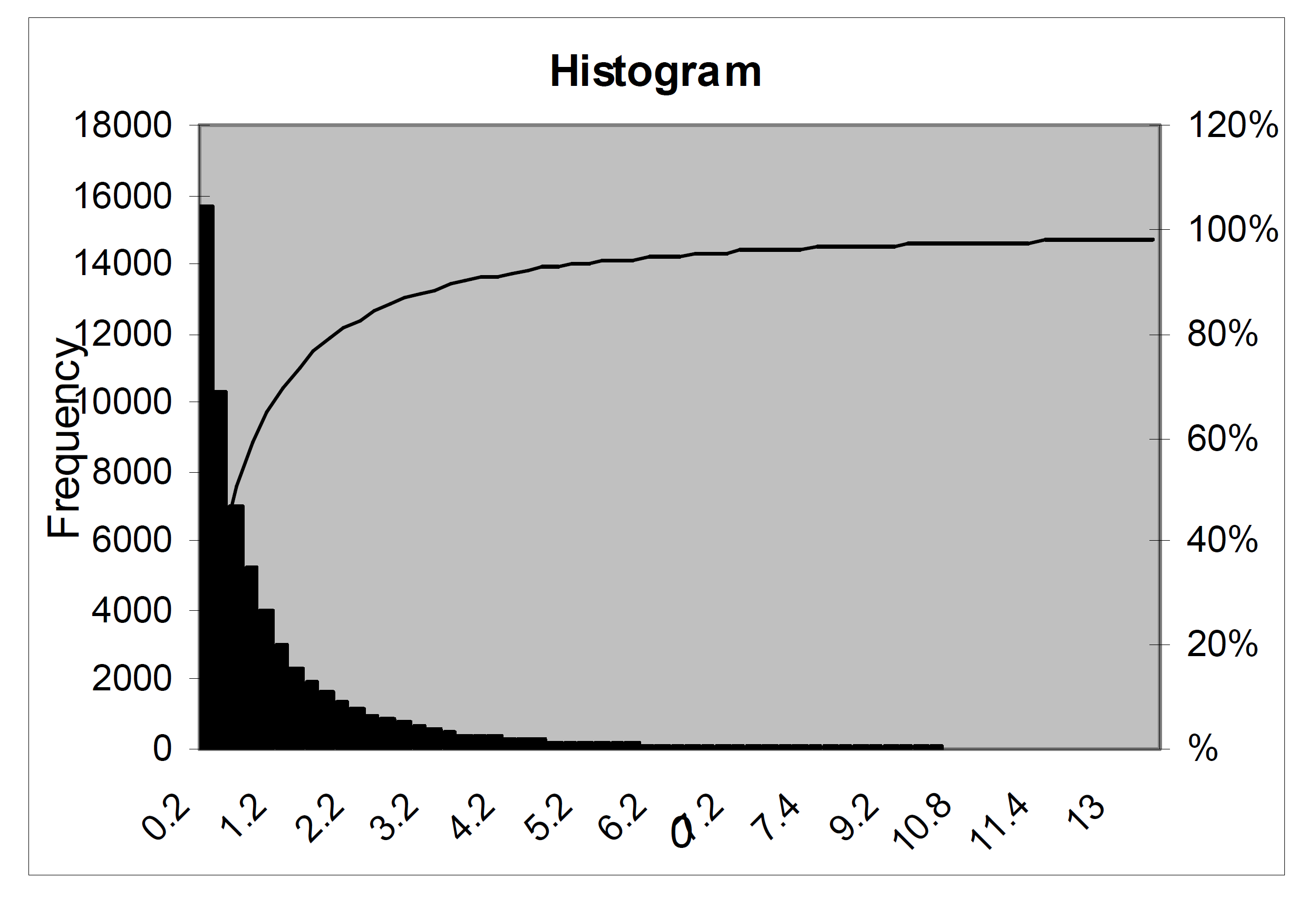
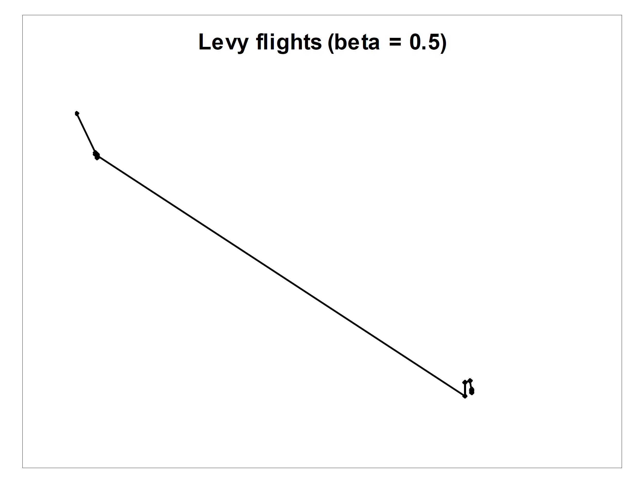
(a) $\beta=1.5$	(b) $\beta=0.5$
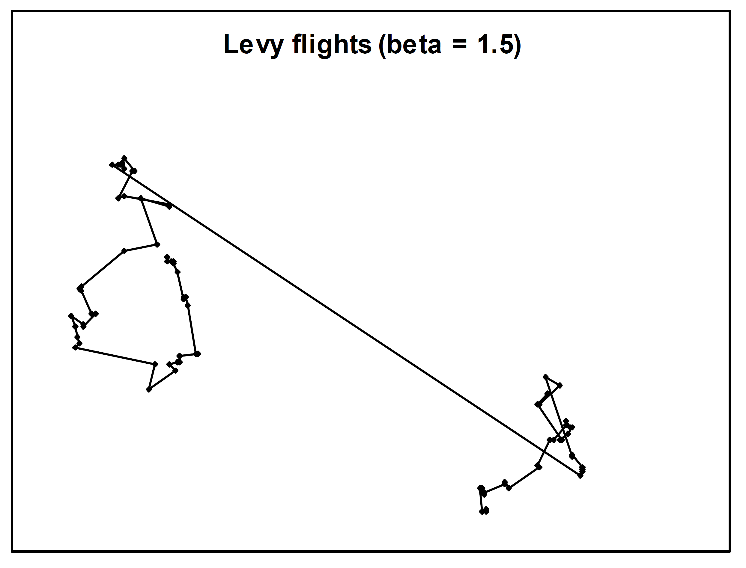
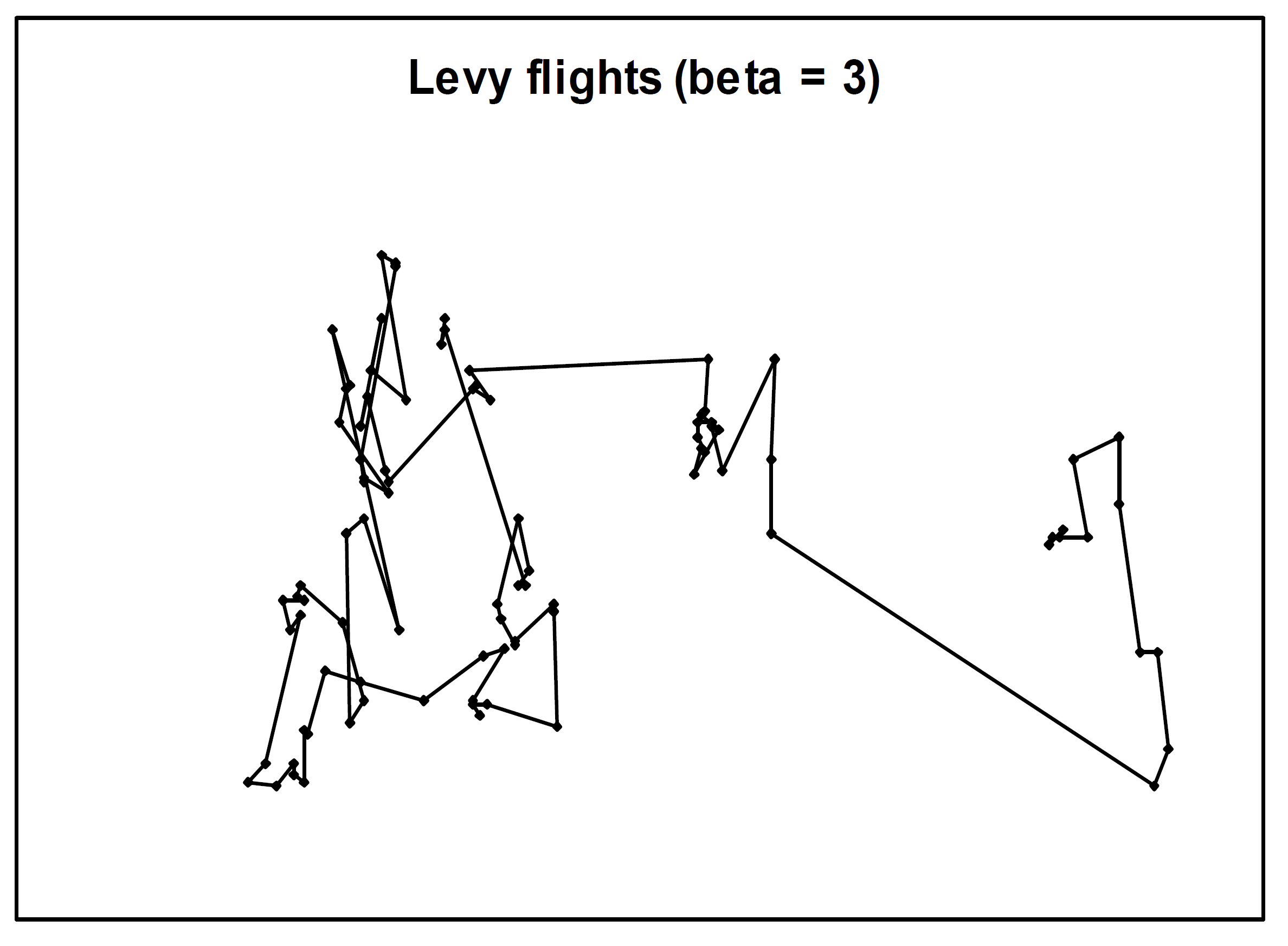
(c) $\beta=1.5$	(d) $\beta=3.0$

Figure 1: Flight length distributions with various $\beta$.

Figs. 1(b-d) show Lévy fights on a 2D landscape with $l_{0}=1$. Note that the scale of Fig. 1(b) is much larger than that of Fig. 1(d) (around order of 102). For small $\beta$, the random walker tends to get crowded around a central location and occasionally jumps a very big step to a new location. As $\beta$ increases, the probability of performing a long jump decreases. Note that Fig. 1(d) shows the random walks as $\beta=3$, which gets outside of the range given in Eq. (1). However, for the computational purposes, we need not to strictly be consistent with physics laws.

3 Algorithms

3.1 Search mechanisms

The goal in optimization is to efficiently explore the search space in order to find globally optimal. Lévy flights provide a mechanism to achieve this goal. We use the term “particle” to call the abstract entity that moves on the search landscape. From each position, the particle can “fly” to a new feasible position at a distance, which is randomly generated from Lévy flights distribution. It is known that a good search algorithm often maintains balance between local exploitation and global exploration [7]. Lévy flights offer a nice way: As in Eq. (2), we control the frequency and the length of long jumps by adjusting the parameters $\beta$ and $l_{0}$, respectively. Ideally, algorithms will dynamically tune these two parameters to best fit a given landscape.

There are several ways to formulate an algorithm that employs such Lévy-based distance. Firstly, Lévy flights define a manageable move strategy, which can include small local steps, global jumps and (or) mixing between the two. As the Lévy process can occasionally generate long jumps, it can be employed in the multistart model. Secondly, one can use a single particle (as in Greedy, SA, Tabu Search) [8, 9] or a set of particle(s) (as in GA, Evolution Strategy, Genetic Programming, ACO and Scatter Search) [7] moving over the search space. The third way, and probably the most promising, is to combine generic movement model provided by Lévy flights with other known single-solution, or population-based meta-heuristics. Such combinations could result in more powerful hybrid algorithms than the originals [9].

3.2 LFO algorithms

Here we propose five algorithms under the class of Lévy Flights Optimization (LFO). We first provide the brief description. Pseudocode for the first four algorithms is then given in Algorithms 1–4.

Basic LFO (LFO-B).

This basic algorithm uses a set of particles at each generation. Starting from one best-known location, the algorithm will generate a new generation at distances which are randomly distributed according to Lévy flights. The new generation will then be evaluated to select the most promising one. The process is repeated until stopping criteria are satisfied. The algorithm is quite closed to GA in a way that it iterates through generations of particle population, and at each generation it selects the good individuals for the next step. However, there selection policy in LFO-B is quite simple: only the best of population survives at each iteration.

Hybrid LFO with Local Search (LFO-LS).

This is an extension of LFO-B algorithm, where before the selection is made each particle performs its own search to reach local optima. The selection procedure then locates the best local optima found so far, and Lévy flights mechanism helps escape from such trap. It is open to implement the local search algorithm.

Local Search with Multiple LFO Restarts (LFO-MLS).

This can be viewed as a sequential version of LFO-LS algorithm and actually behaves as a Multi-start Local Search. Here only one particle is used. In each iteration the particle tries local search until getting trapped in local optima. To escape from such trap, it will jump to new location by a step generated from Lévy distribution. The jump is immediately accepted without further selection.

LFO with Iterated Local Search (LFO-ILS).

This is very similar to LFO-MLS except for the local minima escape strategy. Instead of immediately accepting the Lévy-based jump, the algorithm tries a number of jumps until a better solution is found. This behavior is identified as Iterated Local Search [10].

LFO-MLS + SA (LFO-SA).

This is a combination of LFO-MLS and SA separated in time: LFO-MLS is run first, then the SA takes the solution as the starting point. The idea is that LFO algorithms may locate the good solution quickly while SA helps improve the quality in the long run.

procedure: LFO_B()

   init_position();

   while (stopping_criteria_not_met)

      for each member in the new generation

         $l$$\leftarrow$Lévy_flights($l_{0}$,$\beta$);

         jump_randomly_at_distance($l$);

      endfor

      return_to_best_known_position();

   endwhile

endprocedure

Algorithm 1 Basic LFO (LFO-B).

procedure: LFO_LS()

   init_position();

   while (stopping_criteria_not_met)

      for each member in the new generation

         $l$$\leftarrow$Lévy_flights($l_{0}$,$\beta$);

         jump_randomly_at_distance($l$);

         perform_local_search();

      endfor

      return_to_best_known_position();

   endwhile

endprocedure

Algorithm 2 Hybrid LFO with Local Search (LFO-LS).

procedure: LFO_MLS()

   init_position();

   while (stopping_criteria_not_met)

      perform_local_search();

      $l$$\leftarrow$Lévy_flights($l_{0}$,$\beta$);

      jump_randomly_at_distance($l$);

   endwhile

endprocedure

Algorithm 3 Local Search with Multiple LFO Restarts (LFO-MLS).

procedure: LFO_ILS()

   init_position();

   while (stopping_criteria_not_met)

      perform_local_search();

      $l$$\leftarrow$Lévy_flights($l_{0}$,$\beta$);

      while(not found better solution)

         jump_randomly_at_distance($l$);

      endwhile

   endwhile

endprocedure

Algorithm 4 LFO with Iterated Local Search (LFO-ILS).

4 Experiments and Results

4.1 Test problems

Test problems are $f_{0}$ of [11], $f_{2}$ (Rosenbrock’s saddle) and $f_{5}$ (Shekel’s foxholes) in De Jong’s test function suite [1], Rastrigin’s $f_{6}$ [12] and Keane’s Bump [13].

$f_{0}$:

$$f_{0}(x_{1},x_{2},x_{3},x_{4}) = \sum_{i=1}^{4}\begin{cases}\left(t_{i}\mbox{sgn}(z_{i})+z_{i}\right)^{2}cd_{i}&\,\,\mbox{if}\,\left|x_{i}-z_{i}\right|<\left|t_{i}\right|\\ d_{i}x_{i}^{2}&\,\,\mbox{otherwise}\end{cases}$$

where:

$$z_{i} = \left\lfloor\left|\frac{x_{i}}{s_{i}}\right|+0.49999\right\rfloor\mbox{sgn}(x_{i})s_{i}$$

$$s_{i} = 0.2,\,t_{i}=0.05$$

$$d_{i} = \left\{1,1000,10,100\right\}$$

$$c = 0.15$$

$$-1000 \leq x_{i}\leq 1000.$$

$f_{2}$:

$$f_{2}(x_{1},x_{2},...,x_{N}) = \sum_{i=1}^{N-1}\left(100\left(x_{i}^{2}-x_{i+1}\right)^{2}+\left(1-x_{i}\right)^{2}\right)$$

where:

$$-2.048 \leq x_{i}\leq 2.048,\,\,i=1,2,...,N.$$

$f_{5}$:

$$f_{5}(x_{1},x_{2}) = \frac{1}{\frac{1}{500}+\sum_{j=1}^{25}\frac{1}{j+\sum_{i=1}^{2}(x_{i}-a_{ij})^{6}}}$$

$$a_{1j} = \{-32,-16,0,16,32,-32,-16,0,16,32,-32,-16,0,16,32,$$

$$\quad-32,-16,0,16,32,-32,-16,0,16,32\}$$

$$a_{2j} = \{-32,-32,-32,-32,-32,-16,-16,-16,-16,-16,0,0,0,0,0,$$

$$\quad 16,16,16,16,16,32,32,32,32,32\}$$

$$-65.536 \leq x_{i}\leq 65.536,\,i=1,2.$$

$f_{6}$:

$$f_{6}(x_{1},x_{2},...,x_{N}) = 10N+\sum_{i=1}^{N}\left(x_{i}^{2}-10\cos(2\pi x_{i})\right)$$

$$-5.12 \leq x_{i}\leq 5.12$$

Bump:

$$f_{BUMP}(x_{1},x_{2},...,x_{N}) = 1-\frac{\left|\sum_{i=1}^{N}\cos^{4}(x_{i})-2\prod_{i=1}^{N}\cos^{2}(x_{i})\right|}{\sqrt{\sum_{i=1}^{N}ix_{i}^{2}}}$$

$$0 < x_{i}<10;\,\prod_{i=1}^{N}x_{i}>0.75;\,\sum_{i=1}^{N}x_{i}<\frac{15N}{2}$$

Function $f_{0}$ is very difficult to minimize with $10^{20}$ local minima, and $f_{2}$ is also considered to be hard despite of being uni-modal [11]. $f_{6}$ is interesting because of the sinuous component. According to Keane [13], the Bump is a seriously hard test-function for optimization algorithms because the landscape surface is highly “bumpy” with very similar peaks and global optimum is generally determined by the product constraint. Among those functions, $f_{0}$ and $f_{5}$ have fixed dimensions while the rest can be set freely. In our tests, the dimension of 10 is set for $f_{2}$ and $f_{6}$ and of 50 for the Bump.

4.2 Algorithms implementation

We compare four proposed algorithm with the classic SA. This subsection provides greater details in algorithm realization, which can be classified into move strategy, stopping criteria, and algorithm specificity.

Move strategy.

Each move is selected in random directions spanning in all dimensions of search space where move length is measured in Euclidean metric. In the case of infeasible move to the region outside bounded space, two strategies are used: (i) the move selection is repeated until a feasible one is found, and (ii) the move is stopped at the edges. The first strategy is quite intuitive but it may result in many repetitions in case of long Lévy flights. The second gives chance to explore the boundary regions, in which high quality solutions may be found.

Stopping criteria.

The main stopping criteria used in main algorithms are time and the quality of best solution found so far (compared with known optimal one). Another stopping criterion is number of non-improvement moves. This can be either number of steps in neighborhood exploitation or number of jumps in global exploration. The first is used in greedy search, while the second applies for multiple restart type.

Algorithm specificity.

In SA, the initial temperature $T_{0}$ is chosen as 10% of randomly generated initial solution while the stopping temperature $T_{s}$ is fixed at $0.0001$. Although there are no exact reasons for such choice, it is based on author’s experience with SA so that transition probability is always 1 at the beginning and very close to 0 at the end of each run. The cooling schedule is the widely used power type:

$$T(t)=r^{t}T_{0}\,\,\mbox{where}\,\,r=e^{\mbox{ln}(T/T_{0})/t_{m}}$$

and $t_{m}$ is the maximum allocated run time. In all LFO algorithms, we use the power index $\beta=1.5$. The number of jumps is set at 100 for LFO-B and LFO-MLS algorithms, while the jump distance is limited at a half of largest size of search space’s dimensions.

4.3 Results and Discussions

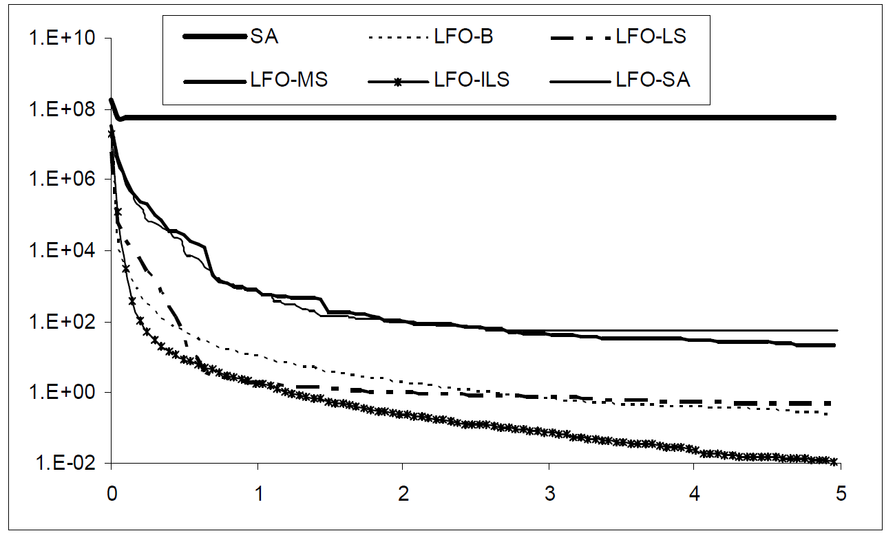
Figure 2: Test results for $f_{0}$.

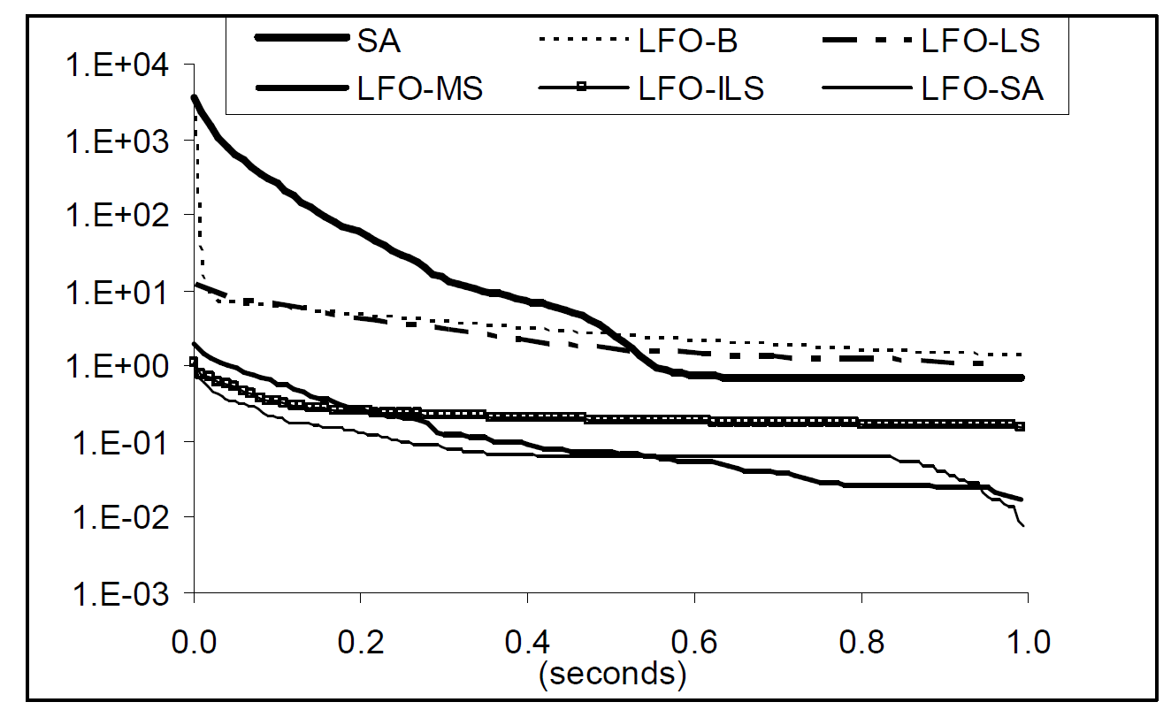
Figure 3: Test results for $f_{2}$.

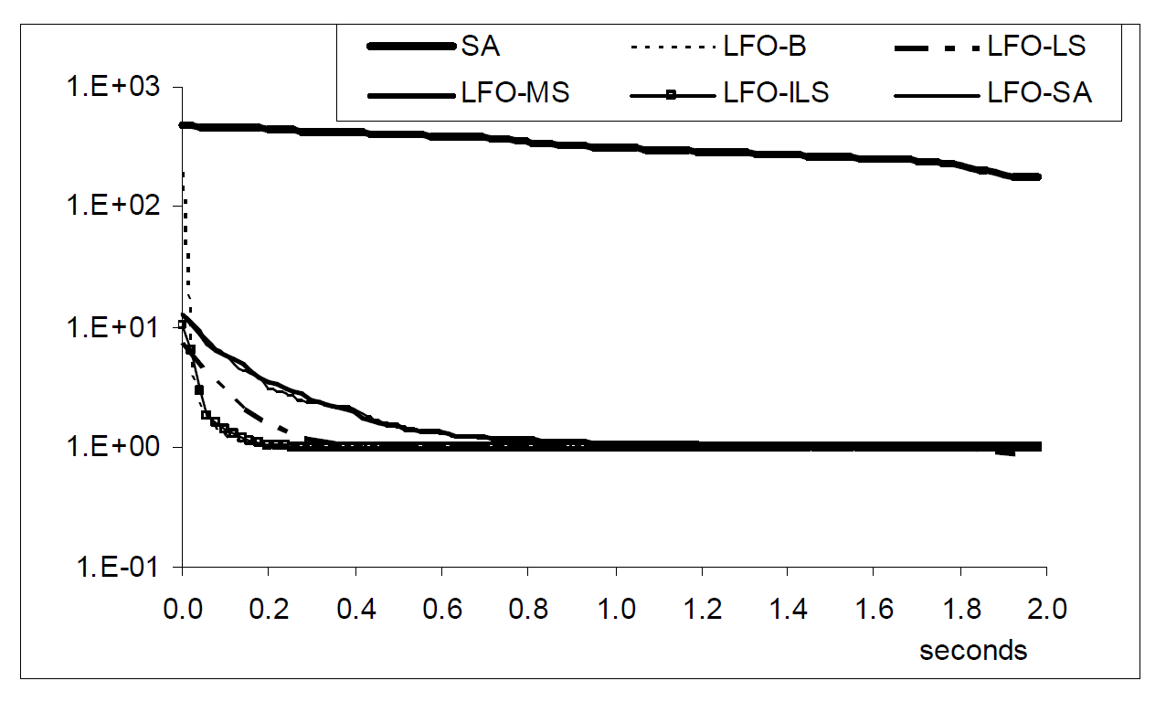
Figure 4: Test results for $f_{5}$.

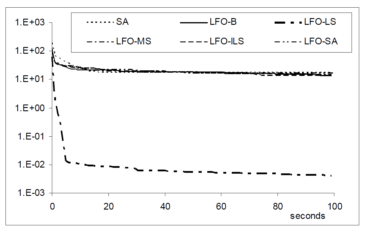
Figure 5: Test results for $f_{6}$.

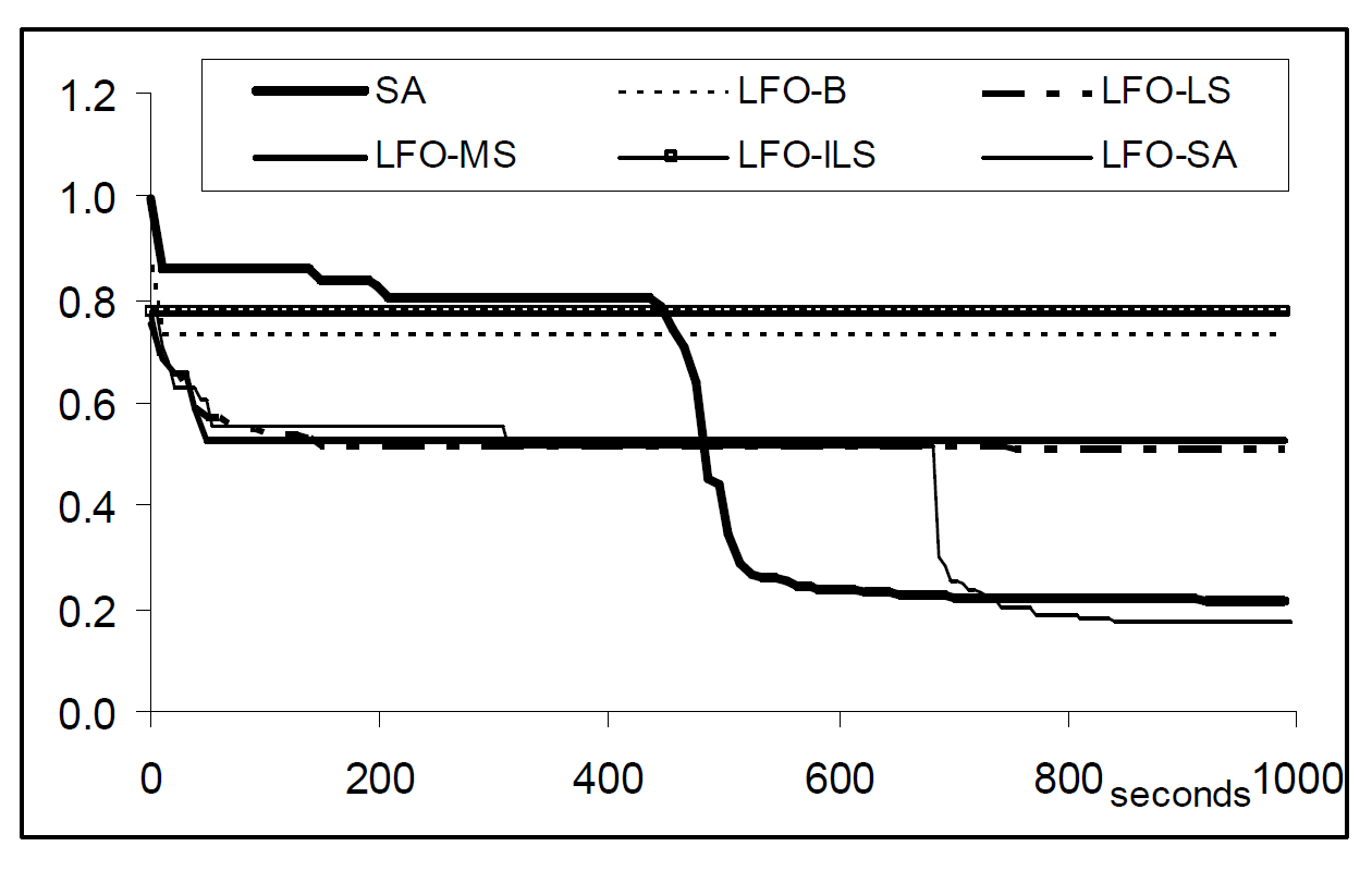
Figure 6: Test results for $f_{6}$.

The tests were run on 2.5GHz Intel computer within given periods of time. Every test was run repeatedly and best found solutions were sampled at relevant intervals and then averaged. Numbers of replications were 100 times for $f_{0}$, $f_{2}$, and $f_{5}$, 20 times for $f_{6}$ and 10 times for the Bump. Algorithms’ performances on the five test problems are presented in Figs. 2–6.

In all cases, some of LFO algorithms outperform SA although SA appears to improve its performance in the long runs. This is a proven beauty of SA but it will be impractical if the required time is too long for daily activities. LFO algorithms tend to sample good quality solutions (compared to initial random solution) very quickly, in most cases within a second. The only exception is the Bump problem, where SA seems to work best after a significant time.

Although there are not enough representative test cases to statistically conclude on the power of LFO algorithms over SA, there are several interesting points to note. Firstly, Lévy flights portrays well the distribution of flight lengths and times performed by foragers observed in natural experiments [5]. In the process of foraging over a given landscape, Lévy distribution helps reduce the probability of returning previously visited locations, compared to normal distribution. This is particularly advantageous in memoryless algorithms like basic stochastic SA or GA, where there are no built-in mechanisms to avoid revisits.

Secondly, as mentioned early in this paper, LFO algorithms work under assumption that good quality solutions can be found around local minima. Such property can be found in most test cases, where experiments have proved the algorithms’ favor. However, in the Bump problem, such “big valley” hypothesis does not hold because the global minimum is located on search space boundary. This property can help explain why LFO algorithms fail to model the Bump landscape structure but succeed in other cases.

Finally, the hybrid LFO-SA appears to work as well as or better SA in all cases while keeping the similar search power to other LFO algorithms. It is obvious that LFO-SA behaves exactly like LFO-MLS in the short run (in $f_{0}$, $f_{2}$, $f_{5}$ and $f_{6}$, see Figs. 2–5) and like SA in the long course (in Bump, see Fig. 6).

5 Conclusions & outlooks

The paper has proposed a set of optimization algorithms based on Lévy flights. The algorithms were validated against Simulated Annealing on several hard continuous test functions. Experiments have demonstrated that LFO (Lévy Flights Optimization) could be superior to SA.

Algorithms implemented in this paper are rather basic, and there are rooms for further extension. For example, the two main parameters of mean Lévy distance and the power index can be adjusted dynamically during the run. Or one may wish to extend the idea of Particle Swarm Optimization (PSO) in the way that the whole population keeps continuous flying while dynamically adjusting speed and direction based on information collected so far. Even each flying particle can be treated as an autonomous agent involving collective intelligent decision making. For those who are familiar with GA, it is possible to extend the practice of GA in the way that at each generation, we select a set of particles in stead of the best one to form the next generation.

References

- [1] K. A. D. Jong, “An analysis of the behavior of a class of genetic adaptive systems,” Ph.D. dissertation, Univ. Michigan, 1975.
- [2] M. Dorigo, V. Maniezzo, and A. Colorni, “Ant system: optimization by a colony of cooperating agents,” Systems, Man, and Cybernetics, Part B: Cybernetics, IEEE Transactions on, vol. 26, no. 1, pp. 29–41, 1996.
- [3] R. C. Eberhart and Y. Shi, “Particle swarm optimization: developments, applications and resources,” in Evolutionary Computation, 2001. Proceedings of the 2001 Congress on, vol. 1. IEEE, 2001, pp. 81–86.
- [4] F. Bardou, “Cooling gases with lévy flights: using the generalized central limit theorem in physics,” arXiv preprint physics/0012049, 2000.
- [5] G. Viswanathan, S. V. Buldyrev, S. Havlin, M. Da Luz, E. Raposo, and H. E. Stanley, “Optimizing the success of random searches,” Nature, vol. 401, no. 6756, pp. 911–914, 1999.
- [6] M. Gutowski, “Lévy flights as an underlying mechanism for global optimization algorithms,” arXiv preprint math-ph/0106003, 2001.
- [7] C. Blum and A. Roli, “Metaheuristics in combinatorial optimization: Overview and conceptual comparison,” ACM Computing Surveys (CSUR), vol. 35, no. 3, pp. 268–308, 2003.
- [8] F. Glover and M. Laguna, Tabu search. Springer, 1999.
- [9] E. Talbi, “A taxonomy of hybrid metaheuristics,” Journal of heuristics, vol. 8, no. 5, pp. 541–564, 2002.
- [10] H. R. Lourenco, O. C. Martin, and T. Stutzle, “Iterated local search,” International Series in Operations Research and Management Science, no. 57, pp. 321–354, 2003.
- [11] A. Corana, M. Marchesi, C. Martini, and S. Ridella, “Minimizing multimodal functions of continuous variables with the ”simulated annealing” algorithm,” ACM Transactions on Mathematical Software (TOMS), vol. 13, no. 3, pp. 262–280, 1987.
- [12] L. D. Whitley, K. E. Mathias, S. B. Rana, and J. Dzubera, “Building better test functions.” in ICGA, 1995, pp. 239–247.
- [13] A. J. Keane, “A brief comparison of some evolutionary optimization methods,” 1996.