KIAS-P14042

Holographic Entanglement Entropy of
Mass-deformed ABJM Theory

Kyung Kiu Kim,¹ O-Kab Kwon,² Chanyong Park,² and Hyeonjoon Shin³

¹Department of Physics and Photon Science, School of Physics and Chemistry,
GIST, Gwangju 500-712, Korea

²Institute for the Early Universe, Ewha Womans University, Seoul 120-750, Korea

³School of Physics, Korea Institute for Advanced Study, Seoul 130-722, Korea

kimkyungkiu@gmail.com, okabkwon@ewha.ac.kr, cyong21@ewha.ac.kr, hyeonjoon@kias.re.kr

Abstract

We investigate the effect of supersymmetry preserving mass deformation near the UV fixed point represented by the ${\cal N}=6$ ABJM theory. In the context of the gauge/gravity duality, we analytically calculate the leading small mass effect on the renormalized entanglement entropy (REE) for the most general Lin-Lunin-Maldacena (LLM) geometries in the cases of the strip and disk shaped entangling surfaces. Our result shows that the properties of the REE in (2+1)-dimensions are consistent with those of the $c$-function in (1+1)-dimensions. We also discuss the validity of our computations in terms of the curvature behavior of the LLM geometry in the large $N$ limit and the relation between the correlation length and the mass parameter for a special LLM solution.

Keywords : entanglement entropy, mass-deformed ABJM theory, LLM geometry
PACS numbers : 11.25.Tq, 11.27.+d, 03.65.Ud

1 Introduction

The entanglement entropy (EE) has become an important quantity in a wide range of research areas, from condensed matter physics to quantum gravity. In quantum field theory, one of its well-known features is the appearance of the area law describing short range correlation in the vicinity of the boundary of two subsystems. This correlation causes the ultra-violet (UV) divergence in the continuum limit, which can be regulated in terms of the UV cutoff [1, 2]. This implies that the EE is a UV sensitive quantity. However, the EE also includes some UV insensitive information for the degrees of freedom related to the long range correlations of the system. One important task for further exploration of such long range degrees of freedom is to define an appropriate finite quantity in the continuum limit, analogous to the Zamolodchikov $c$-function in 2-dimensional quantum field theory [3].

As for the actual computation of the EE itself, it is usually known that it is hard to evaluate the EE when the theory of interest is an interacting one. Actually, the majority of the computations of EE has been done in free field theories. However, the situation changes if a field theory has its gravity dual in the context of AdS/CFT correspondence. According to the suggestion of [4, 5] known as the holographic EE (HEE), the EE of the boundary field theory is given by the minimal surface area in the bulk under the condition that the boundary of the minimal surface is the entangling surface in the boundary theory. Because the HEE concerns only the geometric object, the minimal surface, which is simpler than the direct quantum computation of boundary theory, it can be regarded as a practical way to compute even the EE of interacting field theory, at least in the case where the system is in its ground state.

Among many possible boundary field theories appearing in the AdS/CFT correspondence, those originating from the explicit brane configurations are particularly interesting because they are related to the dual gravity or M/string theory stringently and believed to play any important role in uncovering the nature of AdS/CFT correspondence. One such theory is the $(2+1)$-dimensional $\mathcal{N}=6$ superconformal Chern-Simons matter theory with the gauge group $U(N)_{k}\times U(N)_{-k}$ at Chern-Simons level $k$. It describes the $N$ M2-branes probing a $\mathbf{C}^{4}/\mathbf{Z}_{k}$ orbifold and is called the Aharony-Bergman-Jafferis-Maldacena (ABJM) theory [7]. One feature of this theory is that it allows the supersymmetry preserving mass-deformation [8, 9]. It has been shown in [10] that the gravity dual of the supersymmetric vacua of this mass-deformed ABJM (mABJM) theory for a given $N$ and $k$ is identified with the half-BPS Lin-Lunin-Maldacena (LLM) geometry [11, 12] with SO(2,1)$\times$SO(4)$\times$SO(4) isometry in 11-dimensional supergravity. Interestingly, it was conjectured in [12] that this type of LLM geometry (corresponding to $k=1$ case) is dual to the supersymmetry preserving mass-deformation of the ${\cal N}=8$ CFT, even before the appearance of the ABJM theory.

Since the mABJM theory is a deformation from the conformal ABJM theory, it gives us a chance to study the behviour of the ABJM theory away from the UV conformal fixed point with respect to the change of the deformation parameter. At this point, the EE can be regarded as a good measure for exploring such behaviour. However, since the mABJM theory is highly interacting one, it is practically too hard to compute its EE. Fortunately, the dual geometries corresponding to various supersymmetric vacua have been constructed [13] as alluded to above and thus the HEE can be considered instead of EE.

In this paper, we are interested in the mABJM theory near the UV fixed point. Our main goal is to compute the HEE’s for general supersymmetric vacua and to investigate the effect of the mass deformation from the viewpoint of renormalization group (RG) flow. The RG flow itself is derived from the holographic renormalized EE (REE), which has been proposed by Liu and Mezei [14] to define a UV finite quantity from a given EE. It was shown that the REE for any (2+1)-dimensional Lorentz invariant field theories always monotonically decreases along the RG trajectory [15]. See also [16, 17, 18, 19, 20] for related works. Especially in [20], the present authors have done a study on the topic related with the REE of the mABJM theory, which is a preliminary work of our present work. There, a circle was taken as the entangling surface and the HEE for the most symmetric LLM geometry was calculated. In the present work, we extend the previous one. We study the REE’s of a strip as well as circular shaped entangling surface on the general LLM geometries, which correspond to all possible supersymmetric vacua of the mABJM theory. We also discuss the validity of our computation in terms of gauge/gravity duality in the large $N$ limit.

The organization of this paper is as follows. In the next section, we briefly review the supersymmetric vacuum structure of mABJM theory and the corresponding dual LLM geometry in terms of droplet picture. The HEE of the mABJM theory is studied in Sec. 3. As mentioned above, two types of entangling surface, strip and circular one, are considered. The configuration of droplet we take is quite general except that it represents the weakly curved LLM geometry. Based on the results of HEE, we compute the REE for each entangling surface. Finally, the summary of our results and discussion follow in Sec. 4. In Appendix A, we find the relation between the mass parameter and the correlation length which comes from a cutting off the tip of the minimal surface without mass-deformation. In Appendix B, we discuss the large $N$ behavior of the Ricci scalar at the $y=0$ region.

2 Vacua of the mABJM theory and the LLM geometry

The ${\cal N}=6$ ABJM theory allows the supersymmetry preserving mass deformation [8, 9] by imposing the same mass to 4-complex scalars and their superpartners. One intriguing feature of the mABJM theory is that it has discrete Higgs vacua which are classified by the partition of $N$. Here $N$ is the number of M2-branes in the ABJM theory. The supersymmetric vacua [10] of the mABJM theory with Chern-Simons level $k=1$ have one-to-one correspondence with the Lin-Lunin-Maldacena (LLM) background with SO(2,1)$\times$SO(4)$\times$SO(4) isometry in 11-dimensional supergravity [11, 12]. In this section we briefly review this correspondence and discuss the asymptotic properties of the LLM geometry.

2.1 Supersymmetric vacua of the mABJM theory

In this subsection, we summarize the supersymmetric vacua [10] of the mABJM theory. Before discussing it, we consider the classical vacuum equations, which are obtained by setting the bosonic potential of the mABJM theory to zero [7]. Since the SU(4) global symmetry of the original ABJM theory is broken to SU(2)$\times$SU(2)$\times$U(1) symmetry in the mABJM theory, it is convenient to split the SU(4)-symmetric 4-complex scalars into two SU(2)-symmetric complex scalars, i.e.,

$$Y^{A}=(Z^{a},\,W^{\dagger a}),\qquad Y_{A}^{\dagger}=(Z_{a}^{\dagger},\,W^{a}),$$ (2.1)

where $A=1,2,3,4$, $a=1,2$, and $Y_{A}^{\dagger}$ is the Hermitian conjugation of $Y^{A}$. Then the vacuum equations are written as,

$$Z^{a}Z^{\dagger}_{b}Z^{b}-Z^{b}Z^{\dagger}_{b}Z^{a}=-\frac{\mu k}{2\pi}Z^{a},\qquad W^{\dagger a}W_{b}W^{\dagger b}-W^{\dagger b}W_{b}W^{\dagger a}=\frac{\mu k}{2\pi}W^{\dagger a},$$

$$W_{a}Z^{b}W_{b}-W_{b}Z^{b}W_{a}=0,\qquad Z^{b}W_{b}Z^{a}-Z^{a}W_{b}Z^{b}=0.$$ (2.2)

Solutions of these equations in (2.1) have been found in the form of the GRVV matrices [9]. Each vacuum solution is well represented as a direct sum of irreducible rectangular $n\times(n+1)$ matrices, ${\cal M}_{a}^{(n)}$ $(a=1,2)$, and their Hermitian conjugates, $\bar{\cal M}_{a}^{(n)}$,[10, 13]

$${\cal M}_{1}^{(n)} =\left(\begin{array}[]{cccccc}\sqrt{n\!}\!\!\!&0&&&&\\ &\!\sqrt{n\!-\!1}\!\!&\!0&&&\\ &&\ddots&\ddots&&\\ &&&\sqrt{2}&0&\\ &&&&1&0\end{array}\right),\qquad{\cal M}_{2}^{(n)} =\left(\begin{array}[]{cccccc}0&1&&&&\\ &0&\sqrt{2}&&&\\ &&\ddots&\ddots&&\\ &&&0\!&\!\!\sqrt{n\!-\!1}\!&\\ &&&&0&\!\!\!\sqrt{n\!}\end{array}\right).$$ (2.13)

In terms of these matrices, the vacuum solutions are

$$Z^{a} =\sqrt{\frac{\mu k}{2\pi}}\left(\begin{array}[]{c}\begin{array}[]{cccccc}\mathcal{M}_{a}^{(n_{1})}\!\!&&&&&\\ &\!\!\ddots\!&&&&\\ &&\!\!\mathcal{M}_{a}^{(n_{i})}&&&\\ &&&{\bf 0}_{(n_{i+1}+1)\times n_{i+1}}&&\\ &&&&\ddots&\\ &&&&&{\bf 0}_{(n_{f}+1)\times n_{f}}\end{array}\\ \end{array}\right),$$ (2.21)

$$W^{\dagger a} =\sqrt{\frac{\mu k}{2\pi}}\left(\begin{array}[]{c}\begin{array}[]{cccccc}{\bf 0}_{n_{1}\times(n_{1}+1)}&&&&&\\ &\ddots&&&&\\ &&{\bf 0}_{n_{i}\times(n_{i}+1)}&&&\\ &&&\bar{\mathcal{M}}_{a}^{(n_{i+1})}\!\!&&\\ &&&&\!\!\ddots\!&\\ &&&&&\!\!\bar{\mathcal{M}}_{a}^{(n_{f})}\end{array}\\ \end{array}\right),$$ (2.29)

where ${\bf 0}_{i\times j}$ denotes $i\times j$ null matrix. Since $Z^{a}$ and $W^{\dagger a}$ are $N\times N$ matrices for the gauge group ${\rm U}(N)\times{\rm U}(N)$, we have the following constraints,

$$\sum_{n=0}^{N-1}\big{[}nN_{n}+(n+1)N_{n}^{\prime}\big{]}=N,\qquad\sum_{n=0}^{N-1}\big{[}(n+1)N_{n}+nN_{n}^{\prime}\big{]}=N,$$ (2.30)

where $N_{n}$ $(N_{n}^{\prime})$ denotes the number of blocks of ${\cal M}_{a}^{(n)}$ $(\bar{\cal M}_{a}^{(n)})$.

Any combination of $(N_{n},\,N_{n}^{\prime})$ satisfying the constraint (2.30) can be the solution of the vacuum equation (2.1). However, it was found that the possible combinations of $(N_{n},N_{n}^{\prime})$ are much more than the number of the expected configurations [9] in dual gravity theory, which are known as the LLM geometries. This problem was resolved by introducing quantum fluctuations to classical vacua. It was found that the occupation numbers for the quantum-level supersymmetric vacua are further constrained by the Chern-Simons level $k$,

$$0\leq N_{n}\leq k,\qquad 0\leq N_{n}^{\prime}\leq k,$$ (2.31)

for every $n$ [10]. Thus, only a subset of classical vacua remains supersymmetric at the quantum level.

2.2 LLM geometry with $\mathbb{Z}_{k}$ quotient

It was already conjectured in [12] that the LLM geometry with SO(2,1)$\times$SO(4)$\times$SO(4) isometry in 11-dimensional supergravity should correspond to the ${\cal N}=8$ effective field theory of M2-branes. Subsequently, there has been much progress in this direction, for instance, explicit matrix representation of discrete vacua [9], supersymmetric vacua [10], one-to-one mapping between the supersymmetric vacua of the mABJM theory and the LLM geometries for general $k$ and $N$ [13], etc.. See also [22, 23] for other developments.

The LLM geometry with ${\mathbb{Z}}_{k}$ quotient is given by

$$ds^{2} =-G_{tt}\left(-dt^{2}+dw_{1}^{2}+dw_{2}^{2}\right)+G_{xx}(dx^{2}+dy^{2})+G_{\theta\theta}ds_{S^{3}/\mathbb{Z}_{k}}^{2}+G_{\tilde{\theta}\tilde{\theta}}ds_{\tilde{S}^{3}/\mathbb{Z}_{k}}^{2}$$ (2.32)

with

$$ds^{2}_{S^{3}/\mathbb{Z}_{k}} =d\theta^{2}+\sin^{2}2\theta\,d\phi^{2}+\big{(}(d\lambda+d\varphi/k)+\cos 2\theta d\phi\big{)}^{2},$$

$$ds^{2}_{\tilde{S}^{3}/\mathbb{Z}_{k}} =d\tilde{\theta}^{2}+\sin^{2}2\tilde{\theta}\,d\tilde{\phi}^{2}+\big{(}(-d\lambda+d\varphi/k)+\cos 2\tilde{\theta}d\tilde{\phi}\big{)}^{2},$$

where

$$-G_{tt} =\left(\frac{4\mu_{0}^{2}y\sqrt{\frac{1}{4}-z^{2}}}{f^{2}}\right)^{2/3},$$

$$G_{xx} =\left(\frac{f\sqrt{\frac{1}{4}-z^{2}}}{2\mu_{0}y^{2}}\right)^{2/3},$$

$$G_{\theta\theta} =\left(\frac{fy\sqrt{\frac{1}{2}+z}}{2\mu_{0}\left(\frac{1}{2}-z\right)}\right)^{2/3},$$

$$G_{\tilde{\theta}\tilde{\theta}} =\left(\frac{fy\sqrt{\frac{1}{2}-z}}{2\mu_{0}\left(\frac{1}{2}+z\right)}\right)^{2/3},$$

$$f(x,y) =\sqrt{1-4z^{2}-4y^{2}V^{2}}.$$ (2.33)

The mass parameter $\mu_{0}$ corresponds to turning on a non vanishing 4-form field strength. The LLM geometry in (2.32) is completely determined in terms of $z(x,y)$ and $V(x,y)$,

$$z(x,y) =\sum_{i=1}^{2N_{B}+1}\frac{(-1)^{i+1}(x-x_{i})}{2\sqrt{(x-x_{i})^{2}+y^{2}}},$$

$$V(x,y) =\sum_{i=1}^{2N_{B}+1}\frac{(-1)^{i+1}}{2\sqrt{(x-x_{i})^{2}+y^{2}}},$$ (2.34)

where $N_{B}$ is the number of the black droplets and $x_{i}$’s represent the locations of the boundary lines between the black and white strips. The black and white strips in such a droplet representation indicate the $\mp\frac{1}{2}$ values of the function $z$ along the $y=0$ boundary. For the detailed prescription of the droplet representation for general $k$, see [13].

3 HEE of the mABJM Theory

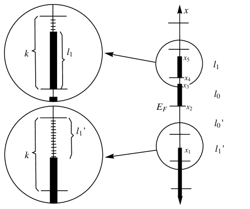
Figure 1: An example for $N_{B}=2$: $E_{F}$ is the Fermi-energy which is the level of black droplet defined when all excited black droplets sink down. The $k$ unit length divides the $x$-axis into sections denoted by indices $n=0,1,2,\ldots$, and each section has $l_{n}$ or $l_{n}^{\prime}$ which is the length of black part or white part, respectively. They are identified with $N_{n}$ and $N_{n}^{\prime}$ describing a field theory vacua.

The LLM geometry introduced in the previous section is asymptotically AdS${}_{4}\times{\rm S}^{7}/{\mathbb{Z}}_{k}$, which means that the conformal symmetry is restored in the UV limit and the dual field theory becomes the ABJM theory without mass deformation. Due to the mass deformation, the conformal symmetry of the system is broken and the dual geometry should be modified in the deep IR region. This correspondence makes it possible to investigate the effect of the mass deformation on the HEE near the UV conformal fixed point of the ABJM theory. Interestingly, it was shown that the REE derived from the HEE at the UV fixed point is consistent with the free energy of the ABJM theory obtained by the localization technique on ${\rm S}^{3}$ [24]. In this section, we compute the HEE and investigate the REE near the UV fixed point of the mABJM theory with a small mass deformation for two types of entangling surface, strip and disk. For consistency check of our results, we will discuss the validity of the dual LLM geometry .

3.1 Strip

First, let us consider the HEE of the strip defined at the boundary of the LLM geometry. Unlike the case of AdS${}_{5}\times S^{5}$, where the role of the compact manifold is trivial, the LLM geometry is not a simple product space so that one should be careful in evaluating the HEE. For the HEE of the strip, we regard a $9$-dimensional surface embedded in the LLM geometry which is called a holographic entangling surface for simplicity. Its boundary of course is identified with the boundary of the strip. If the coordinates of the holographic entangling surface are denoted by $\sigma^{i}$ with $i=1,\cdots,9$, the induced metric can be represented as a functional of the embedding function $X^{M}(\sigma^{i})$

$$g_{ij}=G_{MN}\ \frac{\partial X^{M}\partial X^{N}}{\partial\sigma^{i}\partial\sigma^{j}},$$ (3.35)

where $G_{MN}$ is the $11$-dimensional LLM metric. Then, the surface shape is governed by the following action

$$\gamma_{A}=\int d^{9}\sigma\,\sqrt{\det g_{ij}}.$$ (3.36)

It was conjecture in [4, 5] that the minimal area corresponding to the on-shell action is proportional to the HEE of the strip

$$S_{A}=\frac{{\rm Min}(\gamma_{A})}{4G_{N}}.$$ (3.37)

The boundary space of the LLM geometry can be represented by $R^{1,2}\times S^{7}/\mathbb{Z}_{k}$. If we consider a static strip configuration, it should be extended in the $2$-dimensional noncompact flat space and wrap the $7$-dimensional compact manifold. Let us suppose that the strip is extended in $w_{1}$-direction infinitely and has a finite width $l$ in $w_{2}$-direction. Then, the holographic entangling surface describing the HEE of the strip can be parameterized as follows

$$w_{1}=\sigma^{1},\quad\left(-\frac{L}{2}\leq w_{1}\leq\frac{L}{2}\right),$$

$$w_{2}=\sigma^{2},\quad\left(-\frac{l}{2}\leq w_{2}\leq\frac{l}{2}\right),$$

$$\alpha=\sigma^{3},\,\theta=\sigma^{4},\,\phi=\sigma^{5},\,\tilde{\theta}=\sigma^{6},\,\tilde{\phi}=\sigma^{7},\,\lambda=\sigma^{8},~{}\varphi=\sigma^{9},$$ (3.38)

where the infinite length of $w_{1}$ is regularized to $L$ for convenience. The holographic entangling surface is also extended in the radial direction $r$ which generally becomes a function of the noncompact coordinates. However, the translation symmetry in the $w_{1}$ direction requires $r$ to be a function of $w_{2}$ only, $r=r(w_{2})$.

Substituting the LLM metric into the induced metric formula leads to

$$ds^{2}=|G_{tt}|(dw_{1})^{2}+(|G_{tt}|+G_{xx}r^{\prime 2})(dw_{2})^{2}+G_{xx}r^{2}d\alpha^{2}+G_{\theta\theta}ds^{2}_{S^{3}/\mathbb{Z}_{k}}+G_{\tilde{\theta}\tilde{\theta}}ds^{2}_{\tilde{S}^{3}/\mathbb{Z}_{k}}.$$ (3.39)

Then the action of the holographic entangling surface, after performing the integrations over all angles but $\alpha$, reduces to

$$\gamma_{A}=\frac{4\pi^{4}L}{k}\int_{-l/2}^{l/2}dw_{2}\int_{0}^{\pi}d\alpha~{}r\sqrt{\left|G_{tt}\right|G_{xx}G_{\tilde{\theta}\tilde{\theta}}{}^{3}G_{\theta\theta}{}^{3}\left(\left|G_{tt}\right|+G_{xx}r^{\prime 2}\right)}\ ,$$ (3.40)

where the prime means a derivative with respect to $w_{2}$. Note that $x$, $y$ and $r$ have length square dimension. Let us introduce two dimensionless variables and a new radial coordinate with length dimension

$$\tilde{x}=\frac{4x}{R^{2}}\quad,\quad\tilde{y}=\frac{4y}{R^{2}}\quad{\rm and}\quad u=\frac{R^{3}}{4r},$$ (3.41)

which are related to each other as follows:

$$\tilde{x}=\frac{R}{u}\cos\alpha\quad{\rm and}\quad\tilde{y}=\frac{R}{u}\sin\alpha\ .$$ (3.42)

By using the relation between parameters

$$R=(32\pi^{2}k\tilde{N})^{1/6}l_{\rm P},$$ (3.43)

the action can be rewritten as

$$\gamma_{A} =\frac{\pi^{4}LR^{9}}{32k\mu_{0}}\int_{-l/2}^{l/2}dw_{2}\int_{0}^{\pi}d\alpha\,\frac{f\ \sin^{2}\alpha}{u^{3}}\sqrt{1+\frac{f^{2}u^{\prime 2}}{4\mu_{0}^{2}\sin^{2}\alpha\,u^{2}}}\ ,$$ (3.44)

with

$$f =\sqrt{1-4z^{2}-4y^{2}V^{2}}\,,$$

$$z =\sum_{i=1}^{2N_{B}+1}\frac{(-1)^{i+1}(x-x_{i})}{2\sqrt{(x-x_{i})^{2}+y^{2}}}$$

$$=\frac{1}{2}\left[\cos\alpha+\sum_{k=1}^{\infty}\sum_{i=1}^{2N_{B}+1}\left(\frac{x_{i}}{r}\right)^{k}(-1)^{i+1}\left(P_{1}(\cos\alpha)P_{k}(\cos\alpha)-P_{k-1}(\cos\alpha)\right)\right]\,,$$

$$V =\sum_{i=1}^{2N_{B}+1}\frac{(-1)^{i+1}}{2\sqrt{(x-x_{i})^{2}+y^{2}}}=\frac{1}{2}\sum_{k=0}^{\infty}\sum_{i=1}^{2N_{B}+1}(\frac{1}{r})^{k+1}x_{i}^{k}(-1)^{i+1}P_{k}(\cos\alpha)\,,$$ (3.45)

where $N_{B}$ is the number of black droplets.

Generally speaking, the Lagrangian density for the minimal surface is very complicated in the full LLM geometry and so it is hard to avoid difficulty in performing angle integration. However, our main goal is to see the small mass deformation effect. For this, it is enough to take into account the limit $\mu_{0}\ll r$ rather than the full geometry. In this approximation the mass deformation effect on the HEE appears as deviation from the HEE obtained in AdS₄. More specifically, using (3.45), the function $f$ in the small mass limit is expanded as follows.

$$f=D_{0}\,\mu_{0}\,u\sin\alpha\left[1+D_{1}\,\mu_{0}\,u\cos\alpha+(D_{2}+D_{3}\,\cos(2\alpha))\,\mu_{0}^{2}\,u^{2}+{\cal O}(\mu_{0}^{3})\frac{}{}\right],$$ (3.46)

where

$$D_{0}=\sqrt{2}\sqrt{C_{2}-C_{1}^{2}}~{},~{}D_{1}=-\frac{\left(C_{1}C_{2}-C_{3}\right)}{\sqrt{2}}~{},$$

$$D_{2}=\frac{1}{16}\left(-5C_{2}^{2}-2\left(C_{3}-C_{1}C_{2}\right){}^{2}-4C_{1}C_{3}+9C_{4}\right)~{},$$

$$D_{3}=\frac{1}{16}\left(-3C_{2}^{2}-2\left(C_{3}-C_{1}C_{2}\right){}^{2}-12C_{1}C_{3}+15C_{4}\right)~{}.$$ (3.47)

The coefficient $C_{k}$ appearing in the above formula is defined as

$$C_{k}=\sum_{i=1}^{2N_{b}+1}(-1)^{i+1}\left(\frac{\hat{x}_{i}}{\sqrt{Nk}}\right)^{k},$$ (3.48)

and satisfies $\left(C_{2}-C_{1}^{2}\right)=2$. Here $\hat{x}_{i}$ is defined as $x_{i}=2\pi l_{p}^{3}\mu_{0}\hat{x}_{i}$. When the Chern-Simon level $k$ is equal to 1, a vacuum of the mass deformed ABJM theory can be represented by a Young diagram with $\hat{x}_{i}$, whose area is given by $N$. This area implies the number of M2-branes [12].

Figure 2: k=1 case : The area of the Young-diagram is given by $\left(2\pi\mu_{0}l_{p}^{3}\right)^{2}N$.

Expanding the action with the small $\mu_{0}$, one can easily perform integration for the angle $\alpha$. Up to $\mu_{0}^{2}$ order, $\gamma_{A}$ is expanded as

$$\gamma_{A}\approx \frac{\pi^{4}LR^{9}}{12k}\int_{-l/2}^{l/2}dw_{2}\left(\frac{\sqrt{u^{\prime 2}+1}}{u^{2}}\right.$$

$$\left.+\frac{\mu_{0}^{2}\left(2\left(D_{1}^{2}+10D_{2}-6D_{3}\right)u^{\prime 4}+3\left(D_{1}^{2}+10D_{2}-6D_{3}\right)u^{\prime 2}+10D_{2}-6D_{3}\right)}{10\left(u^{\prime 2}+1\right)^{3/2}}\right).$$ (3.49)

If we regard $w_{2}$ as time, then $\gamma_{A}$ can viewed as an action of the mechanical problem. Since the Lagrangian is independent on $w_{2}$, one may construct a conserved Hamiltonian as follows.

$$H=-\frac{\pi^{4}LR^{9}}{12ku^{2}\sqrt{u^{\prime 2}+1}}-\frac{\pi^{4}\mu_{0}^{2}LR^{9}\left(\left(-3D_{1}^{2}+10D_{2}-6D_{3}\right)u^{\prime 2}+10D_{2}-6D_{3}\right)}{120k\left(u^{\prime 2}+1\right)^{5/2}}~{}~{}.$$ (3.50)

At the turning point denoted by $u_{0}$, $u^{\prime}(w_{2})$ vanishes. Applying this condition, the Hamiltonian turns out to be

$$H=-\frac{\pi^{4}LR^{9}}{12ku_{0}^{2}}+\frac{\pi^{4}\left(6D_{3}-10D_{2}\right)\mu_{0}^{2}LR^{9}}{120k}.$$ (3.51)

Comparing above two expressions, $u^{\prime}$ can be written in terms of $u$

$$u^{\prime}=-\frac{\sqrt{u_{0}^{4}-u^{4}}}{u^{2}}+\frac{\mu_{0}^{2}\left(-3D_{1}^{2}u^{10}+\left(3D_{1}^{2}-10D_{2}+6D_{3}\right)u_{0}^{4}u^{6}+2\left(5D_{2}-3D_{3}\right)u_{0}^{10}\right)}{10u^{2}u_{0}^{4}\sqrt{u_{0}^{4}-u^{4}}}$$ (3.52)

By integration of this equation, the width $l$ and the minimal area $\gamma_{A}$ are presented as functions of $u_{0}$ up to $\mu_{0}^{2}$ order,

$$l= \sqrt{\frac{2}{\pi}}u_{0}\Gamma\left(\frac{3}{4}\right)^{2}$$

$$+\frac{\mu_{0}^{2}u_{0}\left(5\left(3D_{1}^{2}+35D_{2}-21D_{3}\right)u_{0}^{2}\Gamma\left(\frac{1}{4}\right)\Gamma\left(\frac{5}{4}\right)+21\left(3D_{3}-5D_{2}\right)u_{0}^{2}\Gamma\left(\frac{3}{4}\right)^{2}\right)}{105\sqrt{2\pi}},$$

$$\gamma_{A}= \frac{\pi^{4}L\text{ }R^{9}}{6k}\text{ }\left(\frac{1}{\epsilon}-\frac{\Gamma\left(\frac{3}{4}\right)^{2}}{\sqrt{2\pi}u_{0}}+\frac{\mu_{0}^{2}u_{0}\left(15D_{1}^{2}\Gamma\left(\frac{1}{4}\right)^{2}+7\left(5D_{2}-3D_{3}\right)\left(5\Gamma\left(\frac{1}{4}\right)^{2}-4\Gamma\left(\frac{3}{4}\right)^{2}\right)\right)}{280\sqrt{2\pi}}\right),$$ (3.53)

where $\epsilon$ denotes a UV cutoff. Substituting $u_{0}$ into $\gamma_{A}$, the strip entanglement entropy up to $\mu_{0}^{2}$ order reads in terms of $l$

$$S_{A}=\frac{\gamma_{A}}{4G_{N}}=\frac{\pi^{4}L\text{ }R^{9}}{24G_{N}k}\left(\frac{1}{\epsilon}-\frac{\Gamma\left(\frac{3}{4}\right)^{4}}{\pi l}-\mu_{0}^{2}l\frac{\left(21D_{3}-3D_{1}^{2}-35D_{2}\right)\Gamma\left(\frac{1}{4}\right)^{4}}{336\pi^{2}}\right),$$ (3.54)

where $G_{N}=(2\pi l_{{\rm P}})^{9}/(32\pi^{2})$ denotes a $11$-dimensional Newton’s constant with the Planck length $l_{{\rm P}}$. The first and second terms on the right had side are consistent with the HEE obtained in AdS₄, as mentioned before, and the third term is the leading correction caused by the mass deformation in the small mass limit. According to [17], we can define a holographic $c$-function of the strip

$${\cal F}_{{\rm strip}}(l) \equiv l^{2}\partial_{l}\hat{S}_{A}$$

$$=\frac{\pi^{3}R^{9}}{24G_{N}k}\left[\Gamma\left(\frac{3}{4}\right)^{4}-\mu_{0}^{2}l^{2}\left(\frac{\pi\,\Gamma\left(\frac{1}{4}\right)^{2}\left(21D_{3}-3D_{1}^{2}-35D_{2}\right)}{168\Gamma\left(\frac{3}{4}\right)^{2}}\right)\right],$$ (3.55)

where $\hat{S}_{A}\equiv S_{A}/L$. If the coefficient of the $\mu_{0}^{2}l^{2}$ is negative, ${\cal F}^{\prime}_{{\rm strip}}(l)$ becomes negative, which implies that the holographic $c$-function monotonically decreases along the RG flow.

For more concrete example, now let us take into account the symmetric configuration where the parameters are given by

$$D_{1}=0,\quad D_{2}=-1/8,\quad{\rm and}\quad D_{3}=9/8.$$ (3.56)

Then the free energy or $c$-function of the symmetric strip reduces to

$${\cal F}_{{\rm strip}}(l)=\frac{\pi^{3}R^{9}\Gamma\left(\frac{3}{4}\right)^{4}}{24kG_{N}}-\mu_{0}^{2}l^{2}\frac{R^{9}\pi^{2}\Gamma\left(\frac{1}{4}\right)^{4}}{288kG_{N}}.$$ (3.57)

In this case the coefficient of the $\mu_{0}^{2}l^{2}$ is a negative number. This fact implies that the holographic $c$-function shows the monotonically decreasing behavior along the RG flow.

Before going to the disk case, we would like to give a comment on another way of the mass deformation. In [5], the authors considered the mass deformation of CFT in a bottom-up approach. So it is meaningful to make a comparison between our top-down result and theirs. We discuss the identification between them in Appendix A.

3.2 Disk

We now turn to the REE of a disk near the UV fixed point. Let us take a circular region with radius $l$ on the two spatial directions of the boundary noncompact manifold. The $9$-dimensional holographic entangling surface with two noncompact directions is embedded into the target space (2.32) as

$$u=u(\rho),\,w_{1}=\rho\cos\sigma^{1},\,w_{2}=\rho\sin\sigma^{1},\,$$

$$\alpha=\sigma^{3},\,\theta=\sigma^{4},\,\phi=\sigma^{5},\,\tilde{\theta}=\sigma^{6},\,\tilde{\phi}=\sigma^{7},\,\lambda=\sigma^{8},~{}\varphi=\sigma^{9},$$ (3.58)

where the radial coordinate of AdS₄ is given by $u=R/\sqrt{\tilde{x}^{2}+\tilde{y}^{2}}$ and is a function only of $\rho$ due to the rotation symmetry in the $(w_{1},w_{2})$ plane. $\alpha=\tan^{-1}(\tilde{y}/\tilde{x})$ is the angle in the $(x,y)$ plane and the range of $\rho$ is given by $0\leq\rho\leq l$. The action describing the holographic entangling surface, after integrating out angular variables of the compact space, reduces to

$$\gamma_{A}=\frac{\pi^{5}R^{9}}{16k\mu_{0}}\int_{0}^{l}d\rho\,\int_{0}^{\pi}d\alpha\,\frac{f\rho\sin^{2}\alpha}{u^{3}}\sqrt{1+\frac{f^{2}u^{\prime 2}}{4\mu_{0}^{2}\sin^{2}\alpha u^{2}}},$$ (3.59)

where the prime means a derivative with respect to $\rho$, and $f$ in the small mass limit is given in (3.46). In this small mass limit, the $\alpha$ integration up to $\mu_{0}^{2}$ order leads to

$$\gamma_{A}=\frac{\pi^{5}R^{9}}{6k}\int_{0}^{l}d\rho\,\rho\,\bigg{[}\frac{\sqrt{1+u^{\prime 2}}}{u^{2}}+\frac{(5D_{2}-3D_{3})\mu_{0}^{2}}{5\left(1+u^{\prime 2}\right)^{3/2}}+\frac{(D_{1}^{2}+10D_{2}-6D_{3})(3u^{\prime 2}+2u^{\prime 4})\mu_{0}^{2}}{10\left(1+u^{\prime 2}\right)^{3/2}}\bigg{]},$$ (3.60)

where the normalization used in the previous section $D_{0}=2$ is adjusted. Note that, unlike the strip case, there is no conserved charge due to the explicit dependence on $\rho$. So we can not apply the method used in the previous section to the disk case. Here we follow a different strategy.

The minimum value of $\gamma_{A}$ is given by the on-shell action. In the $\mu_{0}\to 0$ limit, $\gamma_{A}$ should be reduced to that of the AdS₄ up to an overall factor caused by the volume of the $7$-dimensional compact manifold. In this zero mass limit, it is well-known that a circle appears as a special solution satisfying the boundary conditions, $u^{\prime}(0)=0$ and $u(l)=0$,

$$u_{0}(\rho)=\sqrt{l^{2}-\rho^{2}}.$$ (3.61)

In order to figure out the mass deformation effect near the UV fixed point, we can take into account a small mass perturbation around the known circular solution. The leading contribution appears at $\mu_{0}^{2}$ order, so we take an ansatz

$$u(\rho)=u_{0}(\rho)+(\mu_{0}\,l)^{2}\ \delta u(\rho).$$ (3.62)

Then, the fluctuation field $\delta u$ is governed by an inhomogeneous second order differential equation

$$0= \delta u^{\prime\prime}+\frac{\left(l^{2}-2\rho^{2}\right)}{l^{2}\rho-\rho^{3}}\ \delta u^{\prime}-\frac{2l^{2}}{\left(l^{2}-\rho^{2}\right)^{2}}\ \delta u$$

$$+\frac{D_{1}^{2}\left(-6l^{4}+14l^{2}\rho^{2}-9\rho^{4}\right)-2\left(5D_{2}-3D_{3}\right)l^{2}\left(3l^{2}-2\rho^{2}\right)}{5l^{4}\sqrt{l^{2}-\rho^{2}}},$$ (3.63)

which allows two integration constants. For the fluctuation solution to be determined unambiguously, we must impose two natural boundary conditions. In the asymptotic region ($u\to 0$), the effect of the mass deformation is negligible, so the deformed solution should reduce to the undeformed one, $u(l)=u_{0}(l)$. This fact implies that the fluctuation field $\delta u(l)$ vanishs at the boundary. Assuming that the action in (3.59) is regular, the holographic entangling surface should be smooth. This smoothness, together with the rotational symmetry in the $(w_{1},w_{2})$ plane, enforces $\delta u^{\prime}(0)=0$ at the turning point. Imposing these two boundary conditions fixes the fluctuation field uniquely

$$\delta u(\rho) =\frac{l^{3}}{300\sqrt{1-(\rho/l)^{2}}}\Big{[}18D_{1}^{2}(\rho/l)^{6}-(61D_{1}^{2}+100D_{2}-60D_{3})(\rho/l)^{4}$$

$$+(112D_{1}^{2}+700D_{2}-420D_{3})(\rho/l)^{2}-69D_{1}^{2}-600D_{2}+360D_{3}$$

$$-8(11D_{1}^{2}+125D_{2}-75D_{3})\Big{(}\tanh^{-1}\sqrt{1-(\rho/l)^{2}}+\ln(\rho/l)-\sqrt{1-(\rho/l)^{2}}\Big{)}\Big{]}.$$ (3.64)

In Fig 2. we plot the deformed holographic entangling surface in the symmetric case in which the mass deformation pushes the turning point toward the AdS₄ center.

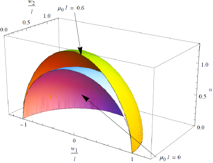
Figure 3: Minimal surfaces for the strip case : The upper surface is a deformed minimal surface due to the mass deformation and the lower surface is for the conformal case

After integrating over $\rho$, the on-shell action up to $\mu_{0}^{2}$ order leads to the HEE of the disk in terms of the radius $l$

$$S_{{\rm disk}}=\frac{\pi^{5}R^{9}}{24kG_{N}}\left(\frac{l}{\epsilon}-1-\frac{75D_{3}-11D_{1}^{2}-125D_{2}}{75}\,(l\mu_{0})^{2}\right),$$ (3.65)

where the UV cutoff in the $u$ coordinate is denoted by $\epsilon$. In the above, the first two terms on the right hand side correspond to the HEE of a disk in the ABJM theory and the last is the first correction caused by the mass deformation. For instance, in the simplest symmetric case of the droplet picture with $k=1$, the parameters $x_{i}$ have

$$x_{1}=-\sqrt{N}\ ,\quad x_{2}=0\ ,\quad{\rm and}\ x_{3}=\sqrt{N},$$ (3.66)

which give rise to $D_{1}=0$, $D_{2}=-1/8$ and $D_{3}=9/8$. Then, the HEE of the symmetric configuration is given by

$$S_{{\rm symm}}=\frac{\pi^{5}R^{9}}{24kG_{N}}\left(\frac{l}{\epsilon}-1-\frac{4}{3}\,(l\mu_{0})^{2}\right).$$ (3.67)

The free energy corresponding to the $c$-function of this system then reduces to

$${\cal F}_{\rm symm}\equiv \left(l\frac{\partial}{\partial l}-1\right)S_{\rm symm}$$

$$= \frac{\pi^{5}R^{9}}{72kG_{N}}\left[3-4(l\mu_{0})^{2}\frac{}{}\right].$$ (3.68)

This result shows that at a given $\mu_{0}$ the free energy decreases along the RG flow when the system size $l$ increases. As expected, this result coincides with the $F$-theorem, ${\cal F}_{\rm symm}^{\prime}<0$.

For general droplets, we finally obtain the REE up to $\mu_{0}^{2}$ order

$${\cal F}_{{\rm disk}}(l)={\cal F}_{ABJM}-\frac{\pi^{5}R^{9}(75D_{3}-11D_{1}^{2}-125D_{2})}{1800kG_{N}}\,(l\mu_{0})^{2},$$ (3.69)

where ${\cal F}_{ABJM}=\frac{\pi^{5}R^{9}}{24kG_{N}}$ is the free energy of the original ABJM theory. The REE counts the effective degrees of freedom of a given system at the length scale $l$ and is expected to play a role of a $c$-function in the holographic point of view. Since the mass deformation we consider is a relevant deformation with the dimensionless coupling constant $g=l\mu_{0}$, the monotonic decreasing of the REE along the RG flow is guaranteed by the following relation

$$75D_{3}-11D_{1}^{2}-125D_{2}>0.$$ (3.70)

If this relation is satisfied, our result supports the $F$-theorem in 3-dimensional field theory [25, 26]. In general droplets, it seems to be difficult to prove the above inequality. We first take into account the symmetric droplet configurations. In these cases, the validity of the dual LLM geometry, as will be shown in the next subsection, depends on the parameter regions. In the regions where the dual LLM geometry is weakly curved, the above inequality is really satisfied. As a result, the REE in (3.69) shows the desired holographic $c$-function behavior near the UV fixed point and, as the system size $l$ increases, monotonically decreases consistently with the $F$-theorem along the RG flow.

3.3 Validity

The results of REE given in (3.55) and (3.69) are for general LLM geometries near the UV fixed point for the strip and the disk cases, respectively. To guarantee their validity, we have to check whether the LLM geometries we have considered are weakly curved everywhere in the large $N$ limit. Here we sketch the validity of our calculations of the REE in the point of view of the gauge/gravity duality. The validity of the LLM geometry for the symmetric droplet case has already been considered in [23], where it was shown that the magnitude of the curvature scalar is decreasing from the droplet point $y=0$ as $y$ increases. On the contrary, the validation is broken for the cases where the curvature scalar does not decrease and remains constant near $y=0$ in the large $N$ limit. Therefore, in checking the validity, it is sufficient to investigate the behavior of the curvature at the droplet point, $y=0$. Following the same logic, we extend the discussion to more general droplet cases.

Let us consider the general droplet characterized by the data $x_{i}$, which specify $z(x,y)$ and $V(x,y)$ of (2.2) describing the full geometry. As one can find in Appendix B, if a given geometry does not have any strongly curved region, it is represented a droplet whose associated Young-diagram has only the long edges of order $\sqrt{N}$ [23, 20]. If there is a strongly curved region, the validity of the HEE is not guaranteed. As an example we consider the droplet corresponding to the rectangular shaped Young-diagram with sides of lengths $w$ and $b$. By parametrizing the lengths as $w=\frac{\sqrt{N}}{\hat{\sigma}},\,\,b=\hat{\sigma}\sqrt{N}$, (3.47) leads to

$$D_{1}=-\frac{\tilde{\sigma}}{\sqrt{2}},\quad D_{2}=\frac{1}{8}\big{(}\tilde{\sigma}^{2}-1\big{)},\quad D_{3}=\frac{1}{8}\big{(}5\tilde{\sigma}^{2}+9\big{)},$$ (3.71)

where $\tilde{\sigma}=\hat{\sigma}-\frac{1}{\hat{\sigma}}$. Here $k=1$ is taken for simplicity. Using these relations we obtain the REE for the strip and the disk,

$${\cal F}_{{\rm strip}}(l) =\frac{\pi^{3}R^{9}}{24G_{N}}\left[\Gamma\left(\frac{3}{4}\right)^{4}-\frac{\pi\,\Gamma\left(\frac{1}{4}\right)^{2}\left(29\tilde{\sigma}^{2}+112\right)}{672\Gamma\left(\frac{3}{4}\right)^{2}}\,(l\mu_{0})^{2}\right],$$

$${\cal F}_{{\rm disk}}(l) =\frac{\pi^{5}R^{9}}{24G_{N}}\left(1-\frac{103\tilde{\sigma}^{2}+400}{300}\,(l\mu_{0})^{2}\right).$$ (3.72)

From (B.78), we see that the finite $\hat{\sigma}$ gives weakly curved LLM geometry. So we expect that our result given in (3.3) is valid. However, in the case $\hat{\sigma}\sim\sqrt{N}$ or $\hat{\sigma}\sim\frac{1}{\sqrt{N}}$, the curvature scalar near $y=0$ region remains finite in the large $N$ limit. Therefore, the gauge/gravity duality may not be valid anymore. In turn, the leading contributions of the mass-deformation to the REE’s of (3.3) are going to diverge, and thus invalidate the gauge/gravity duality. In conclusion, as we discussed previously, in order to have valid results of HEE we have to consider the Young-diagram including only long edges of order $\sqrt{N}$.

4 Summary

Following the gauge/gravity duality, we have investigated the REE of the mass deformed ABJM theory and its RG flow. To do so, we have taken into account the LLM geometry corresponding to vacua of the mABJM theory which can be reinterpreted as droplets in the droplet picture. In general, the REE crucially depends on the droplet configuration, so it is a formidable take to find the analytic form of the general REE in the entire region. In this paper, we focused on the UV region where, due to the relatively small mass deformation, the perturbative and analytic studies on the mass deformation effect are possible. The entanglement entropy is an important concept to understand the degrees of freedom of a physical system. Interestingly, it was shown that the REE of the disk is associated with the free energy of an odd dimensional quantum field theory. The REE generally depends on the shape of the system we consider so that different shaped-systems result in different REE’s. Here, two types of the REE with the strip and disk shapes have been regarded.

The LLM geometry near the asymptotic boundary can be expanded in terms of the Legendre polynomials. In this region, the REE’s of the strip and disk are given by nontrivial functions of the expansion coefficients. We have shown the explicit dependence of the mass deformation in those two shapes. The first correction of the REE appears at $(l\mu_{0})^{2}$ order, which implies that the variation of the REE with respect to coupling $g=l\mu_{0}$ always vanishes as $l$ goes to zero. Therefore, the REE at the UV fixed point is always stationary. Near the UV fixed point, the variation of the REE explains the nontrivial dependence on the deformation parameter which is related to $c$-functions along the RG flow.

In a simple example with a rectangular shaped Young diagram, if the ratio between width and height is given by $1$ in the large $N$ limit, it describes a symmetric droplet configurations. In this case, the REE’s of the strip and disk have a negative slope. So the free energy corresponding the REE monotonically decreases along the RG flow and satisfies the $F$-theorem. In the asymmetric case slightly deviated from the symmetric one, the ratio runs away from $1$ but still remains a finite value. As expected, this slight modification does not change the desired $F$-theorem behavior. In the droplet configurations largely deviated from the symmetric one where the ratio becomes $0$ or $\infty$, we found that the variation of the REE has still a negative but an infinite slope for $(\mu_{0}l)^{2}$, which breaks the perturbative expansion. In this large asymmetric case, actually the dual LLM geometry becomes highly curved so that the dual gravity description of the mABJM theory is not allowed and we should also be careful in applying the AdS/CFT correspondence. Due to this reason, the appearance of the infinite slope does not indicate the breakdown of the $F$-theorem and non-stationarity of the REE at the UV fixed point. In more general droplet configurations, it is still difficult to say whether the $F$-theorem is still working or not. Even in the parameter regions allowing the dual LLM geometry, it is not clear that the slope of the REE is given by a negative number. It would be interesting to clarify the REE of the general droplet configurations along the RG flow and helpful to understand the $F$-theorem and the property of the REE further. We leave it as a future work.

Appendix A Cutting minimal surface and mass deformation

In [4, 5], the authors suggested a useful method for mass deformation in a bottom-up approach. The idea is to cut off the tip of the minimal surface in the conformal case, denoted by $u_{0}$, where the cut-off scale is interpreted as a correlation length $\xi$($<u_{0}$). According to this idea, the entanglement entropy for the strip is

$$S_{\text{strip},~{}\xi} =2\frac{R^{2}L}{4G_{N}^{(4)}}\int_{\epsilon}^{\xi}du\frac{\sqrt{(\frac{dw_{2}}{du})^{2}+1}}{u^{2}}$$ (A.73)

$$=\frac{R^{2}L}{2G_{N}^{(4)}}\left[\frac{1}{\epsilon}-\frac{1}{\xi}+\sum_{n=1}^{\infty}r_{n}\frac{\xi^{4n-1}}{l^{4n}}\right]~{}.$$

$r_{n}$’s are numerical values, some of which are

$$r_{1}=\frac{2\Gamma\left(\frac{3}{4}\right)^{8}}{3\pi^{2}},~{}r_{2}=\frac{6\Gamma\left(\frac{3}{4}\right)^{16}}{7\pi^{4}},~{}r_{3}=\frac{20\Gamma\left(\frac{3}{4}\right)^{24}}{11\pi^{6}},~{}r_{4}=\frac{14\Gamma\left(\frac{3}{4}\right)^{32}}{3\pi^{8}}~{}~{}.$$ (A.74)

When the correlation length is very close to $u_{0}$, one may take another approximation for (A.73). If we express the correlation length, $\xi\equiv u_{0}(1-\delta^{2})$, in terms of a small parameter $\delta$, then the above entanglement entropy is approximated as

$$S_{\text{strip},~{}\xi}\sim\frac{R^{2}L}{2G_{N}^{(4)}}\left[\frac{1}{\epsilon}-\frac{\Gamma\left(\frac{3}{4}\right)^{4}}{\pi l}-\sqrt{\frac{2}{\pi}}\frac{\Gamma\left(\frac{3}{4}\right)^{2}}{l}\delta+O\left(\delta^{3}\right)\right]\,,$$ (A.75)

where $l$ of (3.53) has been used. Up to a multiplicative overall factor, comparing this with (3.54) gives the following expression for $\delta$

$$\delta=\mu_{0}^{2}l^{2}\frac{\pi^{5/2}\left(21D_{3}-3D_{1}^{2}-35D_{2}\right)}{84\sqrt{2}\Gamma\left(\frac{3}{4}\right)^{6}}\,.$$ (A.76)

This allows us to relate the correlation length $\xi$ of the ABJM theory to the small mass deformation $\mu_{0}$ in the mABJM theory. In the symmetric configuration (3.56), $\delta$ is reduced to

$$\delta=\mu_{0}^{2}l^{2}\frac{\pi^{5/2}}{3\sqrt{2}\Gamma\left(\frac{3}{4}\right)^{6}}\sim 1.21769\mu_{0}^{2}l^{2}\,.$$ (A.77)

Appendix B Curvature Scalar at $y=0$

To figure out the validity of the gauge/gravity duality in the HEE calculation, we investigate the behavior of the curvature for general droplets. As discussed in [23], for some cases the geometry near $y\to 0$ limit is highly curved even in the large $N$ limit. The results of the HEE for these cases are not reliable. In the work [20], the authors concentrated on the LLM geometries corresponding to the case of symmetric droplet represented by a square shaped Young-diagram. Here we generalize this case and investigate the behavior of the curvature at $y=0$ in the large $N$ limit.

The curvature scalar at $y=0$ for general droplet is given by

$$l_{{\rm P}}^{2}{\cal R}(x,y)|_{y=0}=\frac{1}{6\pi^{\frac{2}{3}}}\,\frac{Q(\hat{x})}{P(\hat{x})},$$ (B.78)

where $\hat{x}$ is a rescaled dimensionless coordinate, $\hat{x}=2\pi l_{{\rm P}}^{3}\mu_{0}\,x$, and

$$P =\left[g^{\prime}(g^{\prime}-2g^{2})\right]^{\frac{7}{3}},$$

$$Q =\left[-40g^{4}{g^{\prime}}^{3}-8g^{2}{g^{\prime}}^{4}+6{g^{\prime}}^{5}+40g^{3}{g^{\prime}}^{2}g^{\prime\prime}-12g{g^{\prime}}^{3}g^{\prime\prime}-4g^{4}{g^{\prime\prime}}^{2}-2g^{2}g^{\prime}{g^{\prime\prime}}^{2}+{g^{\prime}}^{2}{g^{\prime\prime}}^{2}\right].$$ (B.79)

The curvature scalar is determined by the function $g(\hat{x})$,

$$g(\hat{x})=\frac{1}{2}\left(\sum_{i=1}^{2j}\frac{(-1)^{i+1}}{\hat{x}-\hat{x}_{i}}-\sum^{\infty}_{i=2j+1}\frac{(-1)^{i+1}}{\hat{x}-\hat{x}_{i}}\right),$$ (B.80)

where $\hat{x}_{2j}\leq\hat{x}\leq\hat{x}_{2j+1}$ in the $j$-th black strip. The rescaled coordinate originates from the quantization condition of the four-form flux [13],

$$x_{i+1}-x_{i}=2\pi l_{{\rm P}}^{3}\mu_{0}(\hat{x}_{i+1}-\hat{x}_{i})=2\pi l_{{\rm P}}^{3}\mu_{0}\,{\mathbb{Z}},$$ (B.81)

where ${\mathbb{Z}}$ represents an integer and hence $\hat{x}_{i}$’s can be set to integers. Then the number of M2-branes is represented in terms of $\hat{x}_{i}$ as

$$N=\frac{1}{2}\left(\sum_{i=1}^{\infty}(-1)^{i+1}\hat{x}_{i}^{2}-\sum_{i=1}^{\infty}\sum_{j=1}^{\infty}(-1)^{i+j}\hat{x}_{i}\hat{x}_{j}\right).$$ (B.82)

In the Young-diagram representation, $N$ corresponds to the area of a given diagram.

To obtain reliable results from the gauge/gravity duality, the dimensionless quantity $l_{{\rm P}}^{2}{\cal R}$ should be smaller than $1$ everywhere in the large $N$ limit. Now we investigate the behavior of $l_{{\rm P}}^{2}{\cal R}(x)$ in two representative cases.

(i) $\hat{x}_{1}=-a,\,\,\hat{x}_{2}=0,\,\,\hat{x}_{3}=b$, $\hat{x}_{4}=\hat{x}_{5}=\cdots=0$ case:
In this case $g(\hat{x})$ is given by

$$g(\hat{x})=\frac{1}{2}\left(\frac{1}{\hat{x}+a}-\frac{1}{\hat{x}}-\frac{1}{\hat{x}-b}\right).$$ (B.83)

Eq. (B.82) tells us the relation $N=ab$ with the range $1\leq a,b\leq N$. Let us look at the curvature scalar at the boundary of the black and white droplet and at the middle of the black droplet. For convenience, let us set $a=\alpha\sqrt{N}$ with a constant $\alpha$ with the range, $\frac{1}{\sqrt{N}}\leq\alpha\leq\sqrt{N}$. For finite value of $\alpha$, the curvature behaves as $l_{{\rm P}}^{2}{\cal R}\sim N^{-\frac{1}{3}}$ in the large $N$ limit. On the other hand, in the large value of $\alpha$, the leading contribution to the curvature scalar is given by

$$l_{{\rm P}}^{2}{\cal R}(0)=\frac{1}{3}\left(\frac{4\alpha}{\pi\sqrt{N}}\right)^{\frac{2}{3}},$$

$$l_{{\rm P}}^{2}{\cal R}\big{(}\frac{b}{2}\big{)}=\left(\frac{2\alpha}{\pi\sqrt{N}}\right)^{\frac{2}{3}}.$$ (B.84)

When $\alpha\sim\sqrt{N}$, the curvature scalar is non-vanishing in the large $N$ limit. That is, we see that the corresponding LLM geometry becomes highly curved near $y=0$ and the validity of the gauge/gravity duality is doubtable.

(ii) $\hat{x}_{1}=-a-b,\,\,\hat{x}_{2}=-b,\,\,\hat{x}_{3}=0,\,\,\hat{x}_{4}=c,\,\,\hat{x}_{5}=c+d$ and $\hat{x}_{6}=\hat{x}_{7}=\cdots=0$ case:
Here we set $a=\alpha\sqrt{N}$, $b=\beta\sqrt{N}$, $c=b$, $d=a$ for simplicity. Then due to the relation (B.82), we have the relation $\alpha=\sqrt{\beta^{2}+1}-\beta$ with the range of $\beta$, $\frac{1}{\sqrt{N}}\leq\beta\leq\frac{\sqrt{N}}{2}$. When we consider the curvature scalar on the first black droplet, the $g(\hat{x})$ is given by

$$g(\hat{x})=\frac{1}{2}\left(\frac{1}{\hat{x}+a+b}-\frac{1}{\hat{x}+b}-\frac{1}{\hat{x}}+\frac{1}{\hat{x}-c}-\frac{1}{\hat{x}-b-c}\right)\,.$$ (B.85)

In the small $\beta$ limit near $\hat{x}=0$, the leading contribution to the curvature scalar is given by

$$l_{{\rm P}}^{2}{\cal R}(0)=\frac{1}{3}\left(\frac{2}{\pi\beta\sqrt{N}}\right)^{\frac{2}{3}}.$$ (B.86)

Therefore, we see that when $\beta\sim\frac{1}{\sqrt{N}}$ the curvature scalar is finite in the large $N$ limit. On the other hand, in the large beta limit, the leading contribution to the curvature scalar is given by

$$l_{{\rm P}}^{2}{\cal R}(0)=\frac{4}{3}\left(\frac{\beta}{\pi\sqrt{N}}\right)^{\frac{2}{3}}.$$ (B.87)

We can also obtain the finite curvature scalar in the case of $\beta\sim\sqrt{N}$ in the large $N$ limit.

From the above investigation on the behavior of the curvature scalar for general droplet near $y=0$, we conclude that, in order to obtain a geometry weakly curved everywhere in the large $N$ limit, the length of each edge in the Young-diagram should be proportional to $\sqrt{N}$.

References

- [1] L. Bombelli, R. K. Koul, J. Lee and R. D. Sorkin, “A Quantum Source of Entropy for Black Holes,” Phys. Rev. D 34, 373 (1986).
- [2] M. Srednicki, “Entropy and area,” Phys. Rev. Lett. 71, 666 (1993) [hep-th/9303048].
- [3] A. B. Zamolodchikov, “Irreversibility of the Flux of the Renormalization Group in a 2D Field Theory,” JETP Lett. 43, 730 (1986) [Pisma Zh. Eksp. Teor. Fiz. 43, 565 (1986)].
- [4] S. Ryu and T. Takayanagi, “Holographic derivation of entanglement entropy from AdS/CFT,” Phys. Rev. Lett. 96, 181602 (2006) [hep-th/0603001].
- [5] S. Ryu and T. Takayanagi, “Aspects of Holographic Entanglement Entropy,” JHEP 0608, 045 (2006) [hep-th/0605073].
- [6] T. Nishioka, S. Ryu and T. Takayanagi, “Holographic Entanglement Entropy: An Overview,” J. Phys. A 42, 504008 (2009) [arXiv:0905.0932 [hep-th]]; T. Takayanagi, “Entanglement Entropy from a Holographic Viewpoint,” Class. Quant. Grav. 29, 153001 (2012) [arXiv:1204.2450 [gr-qc]].
- [7] O. Aharony, O. Bergman, D. L. Jafferis and J. Maldacena, “N=6 superconformal Chern-Simons-matter theories, M2-branes and their gravity duals,” JHEP 0810, 091 (2008) [arXiv:0806.1218 [hep-th]].
- [8] K. Hosomichi, K. -M. Lee, S. Lee, S. Lee and J. Park, “N=5,6 Superconformal Chern-Simons Theories and M2-branes on Orbifolds,” JHEP 0809, 002 (2008) [arXiv:0806.4977 [hep-th]].
- [9] J. Gomis, D. Rodriguez-Gomez, M. Van Raamsdonk and H. Verlinde, “A Massive Study of M2-brane Proposals,” JHEP 0809, 113 (2008) [arXiv:0807.1074 [hep-th]].
- [10] H. -C. Kim and S. Kim, “Supersymmetric vacua of mass-deformed M2-brane theory,” Nucl. Phys. B 839, 96 (2010) [arXiv:1001.3153 [hep-th]].
- [11] I. Bena and N. P. Warner, “A Harmonic family of dielectric flow solutions with maximal supersymmetry,” JHEP 0412, 021 (2004) [hep-th/0406145].
- [12] H. Lin, O. Lunin and J. M. Maldacena, “Bubbling AdS space and 1/2 BPS geometries,” JHEP 0410, 025 (2004) [hep-th/0409174].
- [13] S. Cheon, H. -C. Kim and S. Kim, “Holography of mass-deformed M2-branes,” arXiv:1101.1101 [hep-th].
- [14] H. Liu and M. Mezei, “A Refinement of entanglement entropy and the number of degrees of freedom,” JHEP 1304, 162 (2013) [arXiv:1202.2070 [hep-th]].
- [15] H. Casini and M. Huerta, “On the RG running of the entanglement entropy of a circle,” Phys. Rev. D 85, 125016 (2012) [arXiv:1202.5650 [hep-th]].
- [16] I. R. Klebanov, T. Nishioka, S. S. Pufu and B. R. Safdi, “On Shape Dependence and RG Flow of Entanglement Entropy,” JHEP 1207, 001 (2012) [arXiv:1204.4160 [hep-th]].
- [17] I. R. Klebanov, T. Nishioka, S. S. Pufu and B. R. Safdi, “Is Renormalized Entanglement Entropy Stationary at RG Fixed Points?,” JHEP 1210, 058 (2012) [arXiv:1207.3360 [hep-th]].
- [18] M. Ishihara, F. -L. Lin and B. Ning, “Refined Holographic Entanglement Entropy for the AdS Solitons and AdS black Holes,” Nucl. Phys. B 872, 392 (2013) [arXiv:1203.6153 [hep-th]]; T. Nishioka and K. Yonekura, “On RG Flow of for Supersymmetric Field Theories in Three-Dimensions,” JHEP 1305, 165 (2013) [arXiv:1303.1522 [hep-th]]; Y. Bea, E. Conde, N. Jokela and A. V. Ramallo, “Unquenched massive flavors and flows in Chern-Simons matter theories,” JHEP 1312, 033 (2013) [arXiv:1309.4453 [hep-th]]; H. Liu and Mr. Mezei, “Probing renormalization group flows using entanglement entropy,” JHEP 1401, 098 (2014) [arXiv:1309.6935 [hep-th], arXiv:1309.6935].
- [19] T. Nishioka, “Relevant Perturbation of Entanglement Entropy and Stationarity,” arXiv:1405.3650 [hep-th].
- [20] K. K. Kim, O-K. Kwon, C. Park and H. Shin, “Renormalized Entanglement Entropy Flow in Mass-deformed ABJM Theory,” arXiv:1404.1044 [hep-th].
- [21] O. Aharony, O. Bergman and D. L. Jafferis, “Fractional M2-branes,” JHEP 0811, 043 (2008) [arXiv:0807.4924 [hep-th]].
- [22] C. Kim, Y. Kim, O-K. Kwon and H. Nakajima, “Vortex-type Half-BPS Solitons in ABJM Theory,” Phys. Rev. D 80, 045013 (2009) [arXiv:0905.1759 [hep-th]]. R. Auzzi and S. P. Kumar, “Non-Abelian Vortices at Weak and Strong Coupling in Mass Deformed ABJM Theory,” JHEP 0910, 071 (2009) [arXiv:0906.2366 [hep-th]]; A. Hashimoto, “Comments on domain walls in holographic duals of mass deformed conformal field theories,” JHEP 1107, 031 (2011) [arXiv:1105.3687 [hep-th]]; O-K. Kwon and D. D. Tolla, “On the Vacua of Mass-deformed Gaiotto-Tomasiello Theories,” JHEP 1108, 043 (2011) [arXiv:1106.3700 [hep-th]].
- [23] Y. -H. Hyun, Y. Kim, O-K. Kwon and D. D. Tolla, “Abelian Projections of the Mass-deformed ABJM theory and Weakly Curved Dual Geometry,” Phys. Rev. D 87, no. 8, 085011 (2013) [arXiv:1301.0518 [hep-th]].
- [24] A. Kapustin, B. Willett and I. Yaakov, “Exact Results for Wilson Loops in Superconformal Chern-Simons Theories with Matter,” JHEP 1003, 089 (2010) [arXiv:0909.4559 [hep-th]].
- [25] D. L. Jafferis, I. R. Klebanov, S. S. Pufu and B. R. Safdi, “Towards the F-Theorem: N=2 Field Theories on the Three-Sphere,” JHEP 1106, 102 (2011) [arXiv:1103.1181 [hep-th]].
- [26] R. C. Myers and A. Sinha, “Holographic c-theorems in arbitrary dimensions,” JHEP 1101, 125 (2011) [arXiv:1011.5819 [hep-th]].