Hydromagnetic quasi-geostrophic modes in rapidly rotating planetary cores

Abstract

The core of a terrestrial-type planet consists of a spherical shell of rapidly rotating, electrically conducting, fluid. Such a body supports two distinct classes of quasi-geostrophic (QG) eigenmodes: fast, primarily hydrodynamic, inertial modes with period related to the rotation time scale and slow, primarily magnetic, magnetostrophic modes with much longer periods. Here, we investigate the properties of these hydromagnetic quasi-geostrophic modes as a function of non-dimensional parameters controlling the strength of the background magnetic field, the planetary rotation rate, and the amount of magnetic dissipation.

We first present analytic solutions that illustrate the essential parameter dependences of the modes and provide a convenient benchmark for our numerical scheme. A comparison between known three-dimensional inertial modes in a sphere and our axially invariant QG modes shows encouraging agreement at low azimuthal wavenumbers, particularly for the slowest modes. The container geometry and background magnetic field structure are found to influence the radial structure of the modes, but not the scaling of their frequency with the control parameters. When the background magnetic field decreases toward the outer boundary in a spherical shell, QG modes tend to be compressed towards the outer boundary. Including magnetic dissipation, we find a continuous transition from diffusionless slow magnetic modes into quasi-free decay magnetic modes. During that transition (which is controlled by the magnitude of the Elsasser number), we find that slow magnetic modes weakly modified by diffusion exhibit a distinctive spiralling planform. When magnetic diffusion is significant (Elsasser number much smaller than unity), we find quasi-free decay slow magnetic modes whose decay time scale is comparable to, or shorter than, their oscillation time scale.

Based on our analysis, we expect Mercury to be in a regime where the slow magnetic modes are of quasi-free decay type. Earth and possibly Ganymede, with their larger Elsasser numbers, may possess slow modes that are in the transition regime of weak diffusion, depending on the details of their poorly known internal magnetic fields. Fast QG modes, that are almost unaffected by the background magnetic field, are expected in the cores of all three bodies.

1 Introduction

Electrically conducting fluids permeated by magnetic fields support hydromagnetic waves (Alfvén, 1942). These waves play an important dynamical role. They are a means of transporting energy and momentum, and are the natural response of the system to forcing. The cores of terrestrial-type planets, consisting of approximately spherical shells of rapidly-rotating liquid metal, will support such waves provided they also possess an intrinsic magnetic field. Hydromagnetic waves in planetary cores are strongly influenced by rapid rotation which leads to the existence of two classes of waves, one with a time scale comparable to that of the rotation and another class with time scale much longer than that of rotation (Lehnert, 1954; Braginsky, 1964; Hide, 1966). The latter has been proposed as candidates for producing geomagnetic secular variation and may also contribute to the time variations of other planetary magnetic fields. Since planetary cores are closed containers, it is more appropriate to discuss free oscillations (or eigenmodes) rather than progressive waves in an unconfined system; we therefore use the terminology hydromagnetic modes hereinafter.

In this study we determine the hydromagnetic modes for a simple quasi-geostrophic (QG) model of planetary core dynamics, building on the pioneering studies of Hide (1966), Malkus (1967) and Busse (1976). Although hydromagnetic modes are often cited as an important ingredient of planetary core dynamics, there have been surprisingly few studies of them following these early important investigations. The QG model (Busse, 1970; Pais and Jault, 2008; Canet et al., 2009) assumes that disturbances are to leading order invariant parallel to the rotation axis. Studies of three-dimensional instabilities and waves in rapidly-rotating hydromagnetic systems have demonstrated the QG model is a useful approximation provided the period of the disturbance considered is slow compared to the rotation period (Zhang and Fearn, 1994; Gillet et al., 2011) but faster than the magnetic diffusion time scale (Schmitt, 2012).

Our model includes the spherical shell geometry essential for studies of planetary cores, rather than relying on a local $\beta$-plane (Hide, 1966) or annulus (Busse, 1976) approximation or being restricted to a full sphere (Malkus, 1967). Besides assuming it to be uniform (Hide, 1966) or linearly increasing with radius (Malkus, 1967), we also consider the possibility of an underlying azimuthal magnetic field that reaches a maximum value within the shell, in line with the profile found by Gillet et al. (2010) for the cylindrical radial magnetic field. Furthermore, we include realistic levels of magnetic dissipation in the plane perpendicular to the rotation axis where the smallest length scales of the field perturbation are likely to be located. Global mode solutions rather than local solutions are obtained numerically. The investigations presented here are complementary to recent three-dimensional investigations of hydromagnetic modes by Schmitt (2010, 2012) that focused on so-called quasi-free decay modes, which are closely related to the magnetic decay modes of a stationary conductor. In order to concentrate on the intrinsic mode properties, we do not explicitly consider the forcing of the hydromagnetic modes; they may be forced, for example, by convection (e.g. Fearn and Proctor, 1983; Zhang, 1995), shear, or magnetic field instability (e.g. Acheson, 1972; Zhang and Fearn, 1994). Our primary motivation is to better understand the linear dynamics possible within more complete (forced, nonlinear) QG models of rapid core dynamics, currently under development with the aim of modelling geomagnetic secular variation (e.g. Canet et al., 2009).

Laboratory experiments involving rapidly rotating liquid metals permeated by strong magnetic fields also provide compelling evidence for the existence of hydromagnetic modes (Schmitt et al., 2008; Nornberg et al., 2010). The detailed interpretation of these experiments is still under discussion, but it seems that the observed wave-like disturbances are influenced both by the magnetic field and by the rotation of the fluid. There have also been reports that hydromagnetic waves may be responsible for some azimuthal motions of flux patches in numerical geodynamo models (see e.g. Kono and Roberts, 2002). However, both in laboratory experiments and in numerical geodynamo models it has proven difficult to single out the particular wave mechanism at work. Here, by studying a simpler (linear, unforced) problem, and by making the additional assumption that the disturbances are axially invariant, we are able to fully characterize the nature of the oscillations.

Two fundamental non-dimensional parameters are found to control the properties of the hydromagnetic modes in our QG model. The first is the ratio of the rotation time scale over the time scale for Alfvén waves to cross the system, known as the Lehnert number,

$$\mathrm{Le}=\frac{B^{\star}}{\Omega\sqrt{\rho\mu_{0}}r_{o}}.$$ (1)

The second is the ratio between the magnetic diffusion time scale and the time scale of Alfvén waves , known as the Lundquist number

$$\mathrm{Lu}=\frac{r_{o}B^{\star}}{\eta\sqrt{\rho\mu_{0}}}.$$ (2)

Here the outer core radius $r_{o}$ has been taken as the length scale and $B^{\star}$ is the typical magnetic field intensity in the planetary core interior. $\rho$ is the density of the fluid, $\Omega$ is the angular rotation rate, $\mu_{0}$ is the magnetic permeability of free space, and $\eta=1/\sigma\mu_{0}$ is the magnetic diffusivity ($\sigma$ is the electrical conductivity). Table 1 summarizes estimated ranges of the Lehnert and Lundquist numbers for Mercury, Earth and Ganymede. For Earth’s core an upper estimate of the field strength comes from the recent study by Gillet et al. (2010) while for Mercury and Ganymede we use an upper estimate of ten times the observed field value downward continued to the core-mantle boundary (as suggested by the ratio between the mean field strength inside the shell and the surface poloidal field strength typically found in numerical geodynamo models).

	Mercury	Earth	Ganymede
core radius ($\mathrm{m}$)	$1.85\ 10^{6}$ (c) ; $2.02\ 10^{6}$ (i)	$3.48\ 10^{6}$	$4.8\ 10^{5}$ (a)
Field estimate ($\mathrm{T}$)	$\left[1.4\ 10^{-6\ (a)}-1.4\ 10^{-5\ (b)}\right]$	$\left[7.6\ 10^{-4\ (a)}-3\ 10^{-3\ (e)}\right]$	$\left[2.5\ 10^{-4\ (a)}-2.5\ 10^{-3\ (b)}\right]$
Rotation rate(c,a) ($\mathrm{s}^{-1}$)	$1.24\ 10^{-6}$	$7.27\ 10^{-5}$	$1.02\ 10^{-5}$
core density ($\mathrm{kg}/\mathrm{m}^{3}$)	$6980^{(i)}$ ; $8200^{(c)}$	$11000^{(d)}$	$6000^{(d)}$
Electrical resistivity ($\mu\Omega\cdot\mathrm{m}$)	$0.36^{(g)};0.44^{(g)};0.9^{(f)};1.67^{(c)}$	$0.6^{(f)};0.7^{(f)};0.8^{(f)};1.88^{(h)}$	$0.8^{(f)}-5^{(d)}$
Magnetic diffusivity ($\mathrm{m}^{2}/\mathrm{s}$)	$\left[0.29-1.3\right]$	$\left[0.48-1.5\right]$	$\left[0.64-4\right]$
Ekman number $\mathrm{E}$	$2\ 10^{-13}$	$10^{-15}$	$4\ 10^{-13}$
Lehnert number $\mathrm{Le}$	$\left[6\ 10^{-6}-9\ 10^{-3}\right]$	$\left[2.5\ 10^{-5}-10^{-4}\right]$	$\left[5.8\ 10^{-4}-5.8\ 10^{-3}\right]$
Lundquist number $\mathrm{Lu}$	$\left[20-960\right]$	$\left[14,750-186,000\right]$	$\left[345-21,700\right]$
Elsasser number $\mathrm{\Lambda}=\mathrm{Le}\ \mathrm{Lu}$	$\left[1.2\ 10^{-4}-5.4\ 10^{-2}\right]$	$\left[0.4-18.6\right]$	$\left[0.2-125\right]$

Table 1: Estimates of core radius, magnetic field intensity, rotation rate, core density and magnetic diffusivity for the computation of Ekman, Lehnert, Lundquist and Elsasser numbers for Mercury, Earth, and Ganymede. The magnetic field lower estimates are taken from the maximum poloidal field downward continued from observations to the Core-Mantle boundary. The field upper estimates are estimates of the core interior field (from torsional waves studies for Earth, and using a factor 10 between the poloidal and toroidal field estimated from numerical dynamos for Mecury and Ganymede). These ranges of field values lead to the ranges for the Lehnert number. For the computation of the magnetic diffusivities, we use a range of values of electrical resistivity including classical estimates from Stevenson (2003); Wicht et al. (2007); Olson (2007) and recent estimates from first principles calculations of de Koker et al. (2012) (in agreement with Pozzo et al. (2012)) or recent high pressure experiments of Deng et al. (2013). This leads to a range of possible Lundquist numbers. Deng et al. (2013) propose values at $7$ GPa and $1800-2200^{\circ}$C, for Mercury, we have taken De Koker et al.’s value at $7$ GPa and $2000^{\circ}$C, for Earth their values at $130$ GPa and $4000^{\circ}$C or $330$  GPa and $5000^{\circ}$C for Fe, Fe-Si, Fe-O and for Ganymede $10$ GPa and $2000^{\circ}$C (pressure and temperature proposed by Hauck et al. (2006) for a Fe-S composition). For the computation of $\mathrm{E}=\nu/(\Omega r_{0}^{2})$, following Cébron et al. (2012), we take a typical core kinematic viscosity $\nu=10^{-6}$ m²s^-1, consistent with a binary Fe/Fe-S composition. Superscript $(a)$ for estimates from Jones (2003), $(b)$ for ten times the observation based values, following numerical dynamo models. $(c)$ for Wicht et al. (2007), $(d)$ for Stevenson (2003), $(e)$ for Gillet et al. (2010), $(f)$ for de Koker et al. (2012), $(g)$ for Deng et al. (2013), $(h)$ for Olson (2007), $(i)$ for Hauck et al. (2013).

We focus our discussion on the terrestrial-type planets since their interior most likely includes a spherical shell of liquid metal surrounded by a solid silicate layer, and because, as assumed in our model, incompressibility of the liquid layer is likely to be a reasonable approximation. Since Venus and Mars do not presently possess an strong intrinisic field we discuss only Mercury, Earth and Jupiter’s largest moon Ganymede, which also has a dynamo generated internal field. Due to the lack of information concerning the aspect ratio of the inner core to outer core radii in Ganymede and Mercury, only the influence of changing $\mathrm{Le}$ and $\mathrm{Lu}$ (both of which depend on $r_{o}$) is studied here, although the aspect ratio will certainly affect both the period and spatial structure of the eigenmodes. Both the spatial and temporal spectrum of magnetic variations on Earth are now well known (Hulot et al., 2010). The nature of secular variation is currently unknown on Mercury (Anderson et al., 2008, 2012) and on Ganymede (Kivelson et al., 2002). Ambitious orbital missions carrying magnetometers are now planned to survey Mercury (ESA’s Bepi Colombo mission - see Yamakawa et al., 2004) and Ganymede (ESA’s Jupiter Icy Moon Explorer, JUICE, - see Dougherty et al., 2012) so it is of some interest to consider the role hydromagnetic QG modes could play in the magnetic secular variation of these bodies. Crucially, Table 1 shows that the Lehnert number is estimated to be very small for the cores of Mercury, Earth, and Ganymede, implying that rotation dominates magnetic forces for transient motions, suggesting that a QG model is appropriate (Jault, 2008) for studying them. Estimates of the Lundquist number vary by several orders of magnitude, due to uncertainties both in the field strength and in the electrical resistivity of the planetary cores. Nonetheless, it is certainly largest for the Earth and smallest for Mercury. We will show that the Lunquist number plays a crucial role in determining the relevance of slow magnetic QG modes in planetary core dynamics.

This paper is divided into five sections. Section 2 presents the mathematical formulation of our QG model. Section 3 presents an analytic solution describing many essential details of the modes including the splitting into fast and slow modes and the parameter dependence of the dispersion relations. Detailed numerical results are presented in Section 4. These include the influence of spherical geometry, the influence of the background zonal field structure, and the effects of magnetic dissipation on the modes. In Section 5 the implications of our results for planetary core motions and variations in their magnetic fields are discussed. An important comparison of modes periods in the absence of a magnetic field with the analytic full sphere inertial mode solutions is reported in A.

2 Model and methods

2.1 Fluid flow

As illustrated in Figure 1, we consider the dynamics of an incompressible fluid contained in a spherical shell of inner and outer radii $r_{i}$ and $r_{o}$, respectively, assumed to have an Earth-like ratio $r_{i}/r_{o}=0.35$. The background planetary rotation defines what we will refer to as the axial direction, that is the $z$-axis in our working cylindrical coordinate system $(s,\varphi,z)$. Note that we will restrict our attention to the dynamics occurring outside the tangent cylinder, where $r_{i}\leq s\leq r_{o}$, and that we will consider only non-zonal motions.

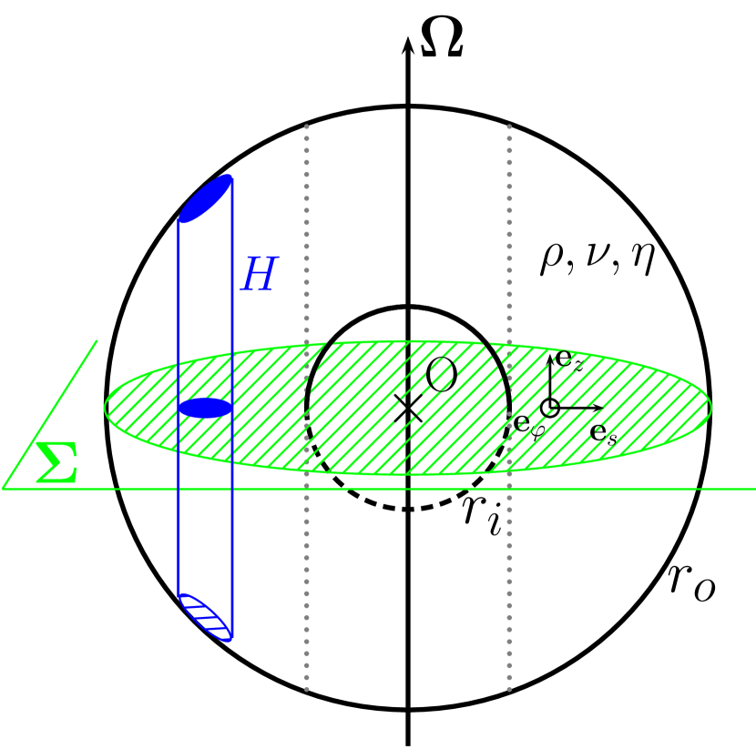
Figure 1: Side view of a planetary core. $\Sigma$ is the equatorial plane and the core-mantle boundary is the outer sphere, located at $r=r_{o}$. $r_{i}$ is the radius of the inner core. $\rho,\nu,\eta$ define the fluid density, viscosity and magnetic diffusivity. Dotted lines defines the cylinder tangent to the inner core. The column of height $2H$ illustrates an example columnar flow element (see text).

We are interested in the combined effect of rotation and magnetic forces on the dynamical behaviour of this system. This behaviour is governed by the Navier–Stokes equation

$$\rho\left(\frac{\mathrm{d}}{\mathrm{d}t}{\mathbf{u}}+2\boldsymbol{\Omega}\times{\mathbf{u}}\right)=-\boldsymbol{\nabla}\Pi+\rho\nu\nabla^{2}{\mathbf{u}}+\frac{1}{\mu_{0}}{\mathbf{B}}\cdot{\boldsymbol{\nabla}}{\mathbf{B}},$$ (3)

in which $\mathrm{d}/\mathrm{d}t$ designates the full material derivative, and ${\mathbf{u}}$, $\Pi$ and $(1/\mu_{0}){\mathbf{B}}\cdot{\boldsymbol{\nabla}}{\mathbf{B}}$ denote the fluid velocity, the modified pressure field and the magnetic tension, respectively (the magnetic pressure component of the Lorentz force has been absorbed into the modified pressure field). This equation has to be supplemented by boundary conditions (which we will specify below), and is completed by the equation for mass conservation, assuming incompressibility,

$$\boldsymbol{\nabla}\cdot{\mathbf{u}}=0.$$ (4)

The Lehnert number $\mathrm{Le}$ defined by (1) above quantifies the importance of rotation compared to magnetic effects in transient motions. Jault (2008) and Gillet et al. (2011) showed in a series of numerical experiments that, if $\mathrm{Le}\lesssim 10^{-2}$, transient motions possess a substantial degree of axial invariance. Since the Lehnert number can be understood as the ratio of the time scale of inertial waves to the time scale of Alfvén waves, small Lehnert number means that inertial waves react and communicate information from perturbations faster than Alfvén waves. This enables a relaxation towards axial invariant geostrophy, despite the presence of magnetic forces. The values of $\mathrm{Le}$ reported in Table 1 for the Earth, Ganymede and Mercury are well below the $10^{-2}$ threshold; this motivates us to introduce a quasi-geostrophic description of the fluid motions, by decomposing the flow ${\mathbf{u}}$ and modified pressure $\Pi$ into a geostrophic component $({\mathbf{u}}^{g},\Pi^{g})$ and a non-geostrophic component $({\mathbf{u}}^{a},\Pi^{a})$, according to

$${\mathbf{u}} = {\mathbf{u}}^{g}+{\mathbf{u}}^{a},$$ (5)

$$\Pi = \Pi^{g}+\Pi^{a}.$$ (6)

Our framework assumes that the main balance is geostrophic

$$2\rho\boldsymbol{\Omega}\times{\mathbf{u}}^{g}=-\boldsymbol{\nabla}\Pi^{g},$$ (7)

and that departures from this balance are described by

$$\rho\left(\frac{\mathrm{d}}{\mathrm{d}t}{\mathbf{u}}^{g}+2\boldsymbol{\Omega}\times{\mathbf{u}}^{a}\right)=-\boldsymbol{\nabla}\Pi^{a}+\rho\nu\nabla^{2}{\mathbf{u}}^{g}+\frac{1}{\mu_{0}}{\mathbf{B}}\cdot{\boldsymbol{\nabla}}{\mathbf{B}}.$$ (8)

The quasi-geostrophic approximation therefore amounts to restricting the contribution of the non-geostrophic components of motion in this last equation to the Coriolis and pressure terms (Gillet et al., 2011). The validity of this approximation has been extensively discussed in the literature (consult for instance Gillet and Jones (2006), Gillet et al. (2011), and references therein). It suffices here to mention that it stands on firm theoretical ground if the slope of the container,

$$H^{\prime}(s)\equiv{\mathrm{d}}H/{\mathrm{d}}s,$$ (9)

remains small. That condition does not hold in a spherical shell, for which

$$H(s)=\sqrt{r_{o}^{2}-s^{2}}.$$ (10)

In practice however, the quasi-geostrophic approximation can remain successful even if ${\mathrm{d}}H/{\mathrm{d}}s\sim 1$ (see Williams et al., 2010).

It is now useful to consider the non-dimensional form taken by (8), taking $B^{\star}$ as the magnetic field scale, the Alfvén wave speed

$$V_{A}\equiv\frac{B^{\star}}{\sqrt{\rho\mu_{0}}}$$ (11)

as the velocity scale, the outer radius $r_{o}$ at the length scale, the Alfvén time

$$T_{A}\equiv\frac{r_{o}}{V_{A}}$$ (12)

as the time scale, and the kinetic pressure $\rho V_{A}^{2}$ as the pressure scale. This yields

$$\frac{\mathrm{d}}{\mathrm{d}t}{\mathbf{u}}^{g}+\frac{2}{\mathrm{Le}}{\mathbf{e}}_{z}\times{\mathbf{u}}^{a}=-\boldsymbol{\nabla}{\Pi^{a}}+\frac{\mathrm{E}}{\mathrm{Le}}\nabla^{2}{\mathbf{u}}^{g}+{\mathbf{B}}\cdot{\boldsymbol{\nabla}}{\mathbf{B}},$$ (13)

where we understand that field variables are now non-dimensional. It appears that viscous forces are proportional to the ratio of the Ekman number $\mathrm{E}$ to the Lehnert number $\mathrm{Le}$. The smallness of $\mathrm{E}$ for the planetary cores of interest here is such that $\mathrm{E}/\mathrm{Le}\ll 1$ (see Table 1). We will therefore neglect viscous forces in the remainder of this study.

By virtue of the geostrophic balance written in (7), the geostrophic flow does not vary along the axial direction. We follow Schaeffer and Cardin (2005) and Canet et al. (2009) and describe it as

$${\mathbf{u}}^{g}(s,\varphi,t)=\frac{1}{H(s)}{\mathbf{e}}_{z}\times\left[\boldsymbol{\nabla}\Psi(s,\varphi,t)\right],$$ (14)

in which $\Psi$ is a time-dependent auxiliary streamfunction defined in the equatorial plane $\Sigma$ (recall Figure 1). This definition, when inserted into (4) for three-dimensional mass conservation, implies a connection between the $z$ component of ${\mathbf{u}}^{a}$ and the equatorial divergence of ${\mathbf{u}}^{g}$, namely that

$$\boldsymbol{\nabla}_{E}\cdot{\mathbf{u}}^{g}\equiv\frac{1}{s}\left[\partial_{s}\left(su_{s}^{g}\right)+\partial_{\varphi}u_{\varphi}^{g}\right]=-\beta u_{s}^{g}=-\partial_{z}u_{z}^{a},$$ (15)

in which

$$\beta(s)\equiv\frac{H^{\prime}(s)}{H(s)}.$$ (16)

The standard quasi-geostrophic approximation omits the $1/H(s)$ prefactor in (14). Consequently, it restricts the conservation of mass to the equatorial plane, and is only fully justified in the small slope situation discussed above. In A, we discuss further how faithfully this version of the quasi-geostrophic model can mimic fully three-dimensional (slow) inertial modes that have been analytically described by Zhang et al. (2001).

We now turn to the vorticity equation and consider the $z$-component of the curl of the axial average of (13) to obtain our working equation. It is expressed here directly in terms of $\Psi$, as

$$\left[\frac{{\mathrm{d}}}{{\mathrm{d}}t}\left(-\nabla^{2}_{E}+\beta\partial_{s}\right)-\frac{2}{\mathrm{Le}}\frac{\beta}{s}\partial_{\varphi}\right]\Psi=H\,{\mathbf{e}}_{z}\cdot\boldsymbol{\nabla}\times\langle\left({\mathbf{B}}\cdot{\boldsymbol{\nabla}}{\mathbf{B}}\right)\rangle,$$ (17)

where $\langle\cdot\rangle$ denotes axial averaging and the equatorial Laplacian $\nabla^{2}_{E}$ is defined by

$$\nabla^{2}_{E}\equiv\frac{1}{s}\partial_{s}s\partial_{s}+\frac{1}{s^{2}}\partial_{\varphi}^{2}.$$ (18)

Within the present inviscid framework, non-penetration at both boundaries implies

$$\Psi(s=r_{i},\varphi,t)=\Psi(s=r_{o},\varphi,t)=0\ \ \forall(\varphi,t).$$ (19)

In addition, notice that our choice of $\Psi$ guarantees that ${\mathbf{u}}\cdot{\mathbf{e}}_{r}=0$ at $z\pm H(s),\ \forall(s,\varphi)$.

As presented here, our description with the auxiliary function $\Psi$ does not account for zonal motions, which are beyond the scope of this study. Their consistent treatment would require the inclusion of the zonally averaged Navier–Stokes equation, following for instance the analysis of Plaut and Busse (2002).

2.2 Magnetic induction

We have deferred until now the discussion of the evolution of the magnetic induction ${\mathbf{B}}$, which is governed by the induction equation

$$\partial_{t}{\mathbf{B}}=\boldsymbol{\nabla}\times\left({\mathbf{u}}\times{\mathbf{B}}\right)+\frac{1}{\mu_{0}\sigma}\nabla^{2}{\mathbf{B}},$$ (20)

under the constraint of conservation of magnetic flux

$$\boldsymbol{\nabla}\cdot{\mathbf{B}}=0.$$ (21)

The induction equation must be complemented by suitable boundary conditions (see below). Its non-dimensional form is obtained using the scales defined above, which lead to

$$\partial_{t}{\mathbf{B}}=\boldsymbol{\nabla}\times\left({\mathbf{u}}\times{\mathbf{B}}\right)+\frac{1}{\mathrm{Lu}}\nabla^{2}{\mathbf{B}},$$ (22)

where, again, we understand that field variables are non-dimensional. Magnetic diffusion scales in inverse proportion to the Lundquist number, previously defined in the introduction, and which expresses the ratio of the magnetic diffusion time scale to the Alfvén wave time scale $T_{A}$. This number is much larger than unity for the systems we are interested in, but the smallness of $1/\mathrm{Lu}$ is by no means comparable to the smallness of the $\mathrm{E}/\mathrm{Le}$ ratio in the Navier–Stokes equation (13). We therefore retain this term in our analysis; in fact, we will show in the following that magnetic diffusion can have dramatic consequences concerning the time-dependence and spatial structure of hydromagnetic QG modes.

A consistent treatment of three-dimensional magnetic induction within the axially-averaged vorticity equation (17) involves consideration of the evolution of three quadratic quantities that stem from the application of axial averaging to the magnetic tension ${\mathbf{B}}\cdot\boldsymbol{\nabla}{\mathbf{B}}$, as described by Canet et al. (2009). Here we instead make a major simplifying assumption, and consider only axially invariant magnetic fields, whose analysis can conveniently be restricted to the equatorial plane $\Sigma$. The motivation behind this step is to obtain physical insight concerning the interaction of the magnetic field and rapidly rotating flow within a simple setting. Furthermore when magnetic diffusion is a secondary effect, one expects perturbations of the magnetic field to follow those of the flow. This assumption is not new; it was made by Busse (1976) in his annulus model of the geodynamo, and more recently by Tobias et al. (2007) in their $\beta$-plane analysis of MHD turbulence in the solar tachocline. Furthermore, this assumption enables us to introduce consistently the effects of magnetic diffusion – the quadratic formalism laid out by Canet et al. (2009) does not easily lend itself to including this important dissipative process.

Our mathematical description of two-dimensional magnetic induction ${\mathbf{B}}$ is analogous to that of the flow, and involves a magnetic potential $A$

$${\mathbf{B}}(s,\varphi,t)=\boldsymbol{\nabla}\times\left[A(s,\varphi,t){\mathbf{e}}_{z}\right].$$ (23)

This assumption allows us to rewrite the induction equation in the following scalar form

$$\partial_{t}A=-{\mathbf{u}}^{g}\cdot\boldsymbol{\nabla}A+\frac{1}{\mathrm{Lu}}\nabla^{2}_{E}A,$$ (24)

in which we notice that solely geostrophic flow interacts with the magnetic potential. In addition, the magnetic tension term ${\mathbf{e}}_{z}\cdot\boldsymbol{\nabla}\times({\mathbf{B}}\cdot{\boldsymbol{\nabla}}{\mathbf{B}})$ in (17) now writes $-{\mathbf{B}}\cdot\boldsymbol{\nabla}(\nabla^{2}_{E}A)$.

2.3 Basic state and modal equations

The modal analysis of interest here requires that we linearize the problem around a basic state, by decomposing

$${\mathbf{u}}(\mathbf{r},t) = \mathbf{U}_{0}(\mathbf{r})+\delta\mathbf{{\mathbf{u}}}(\mathbf{r},t),$$ (25)

$${\mathbf{B}}(\mathbf{r},t) = {\mathbf{B}}_{0}(\mathbf{r})+\delta{\mathbf{B}}(\mathbf{r},t).$$ (26)

We will assume throughout that the basic state is defined by a zero velocity and a zonal magnetic field, whose strength varies with cylindrical radius

$$\mathbf{U}_{0}(\mathbf{r}) = \mathbf{0},$$ (27)

$${\mathbf{B}}_{0}(\mathbf{r}) = B_{0}(s)\mathbf{e}_{\varphi}.\$$ (28)

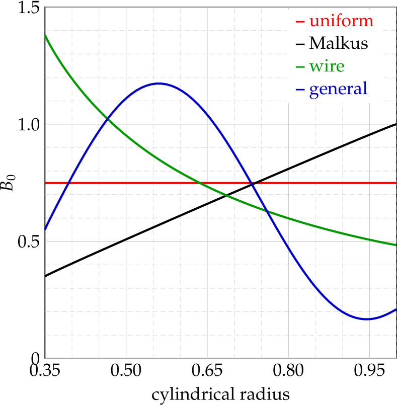
Figure 2: Radial profile of the zonal background fields $B_{0\varphi}$ studied. Red line: uniform toroidal field, black line: toroidal Malkus field (see text), green line: field corresponding to a wire, blue line: a more general zonal background field.

The assumption of a purely zonal background magnetic field is a simplification; in reality the background field within planetary cores will also contain a (cylindrical) radial field which is neglected here to focus attention on the most essential physics. In order to study the impact of the background magnetic field on the catalog of hydromagnetic modes, we shall consider different background magnetic field profiles, as illustrated in Figure 2.

1. A uniform profile (red curve in Figure 2)

   $$B_{0}^{u}(s)=C_{un},$$ (29)

   with $C_{un}$ a constant.

2. The Malkus field, named after the seminal work of (Malkus, 1967) (black curve in Figure 2), which has

   $$B_{0}^{\mathcal{M}}(s)=s.$$ (30)

3. The field created by an electrical wire placed along the $z$-axis (green curve in Figure 2)

   $$B_{0}^{w}(s)=C_{w}/s$$ (31)

   with $C_{w}$ a constant.

4. A more general field, whose variations are non-monotonic (blue curve in Figure 2), and whose non-dimensional expression writes

   $$B_{0}^{g}(s)=C_{g}f(s),$$ (32)

   in which $C_{g}$ is a constant and $f(s)=(3/2)\cos\left[\pi(\alpha_{1}-\alpha_{2}s)\right]+2$, with $\alpha_{1}=3/2$ and $\alpha_{2}=1/0.38$.

The constants $C_{un},C_{w}$, and $C_{g}$ appearing in these expressions are chosen under the constraint of obtaining the same root-mean-square field strength in all cases, and therefore the same definition of the Lehnert number, independent of the background configuration. This leads to $C_{un}=0.75$, $C_{w}=0.48$ and $C_{g}=0.34$.

We proceed by utilizing the scalar functions $\Psi$ and $A$ introduced above in order to describe the perturbations $\delta\mathbf{{\mathbf{u}}}$ and $\delta{\mathbf{B}}$, respectively. In addition, let $A_{0}$ denote the magnetic potential which characterizes ${\mathbf{B}}_{0}$. Upon linearization, (17) and (24) then become

$$\left[\partial_{t}\left(-\nabla^{2}_{E}+\beta\partial_{s}\right)-\frac{2}{\mathrm{Le}}\frac{\beta}{s}\partial_{\varphi}\right]\Psi = \frac{H}{s}\left(-{B_{0}}\partial_{\varphi}\nabla^{2}_{E}-\partial_{s}\nabla^{2}_{E}A_{0}\partial_{\varphi}\right)A,$$ (33)

$$\left(\partial_{t}-\frac{1}{\mathrm{Lu}}\nabla^{2}_{E}\right)A = \frac{B_{0}}{sH}{\partial_{\varphi}}\Psi.$$ (34)

These are supplemented with non-penetration boundary conditions for the flow (19), and vanishing magnetic perturbations at both boundaries, following Busse (1976). This later condition writes

$$A(s=r_{i},\varphi,t)=A(s=r_{o},\varphi,t)=0\ \ \forall(\varphi,t).$$ (35)

We note in passing that setting $A=0$ at the boundaries is equivalent to assuming the boundaries are perfectly conducting.

To carry out a global modal analysis, we consider trial solutions of the form

$$(\Psi,A)(s,\varphi,t)=\mathrm{Re}\left\{\left[\hat{\Psi}(s),\hat{A}(s)\right]\exp\left[-\mathrm{i}\left(m\varphi+\omega t\right)\right]\right\},$$ (36)

where $m$ and $\omega$ are the azimuthal wavenumber and angular frequency of the sought modes, respectively. Inserting this ansatz into (33)-(34) leads to the following system

$$\left[\omega\left(\frac{1}{s}\partial_{s}s\partial_{s}-\frac{m^{2}}{s^{2}}-\beta\partial_{s}\right)+\frac{2}{\mathrm{Le}}\frac{m\beta}{s}\right]\hat{\Psi} = \frac{mH}{s}\left[B_{0}\left(\frac{1}{s}\partial_{s}s\partial_{s}-\frac{m^{2}}{s^{2}}\right)+\partial_{s}\nabla^{2}_{E}A_{0}\right]\hat{A},$$ (37)

$$\left[\omega-\frac{\mathrm{i}}{\mathrm{Lu}}\left(\frac{1}{s}\partial_{s}s\partial_{s}-\frac{m^{2}}{s^{2}}\right)\right]\hat{A} = \frac{mB_{0}}{sH}\hat{\Psi}.$$ (38)

We next approximate the cylindrical radial dependence of $\hat{\Psi}$ and $\hat{A}$ using Chebyshev polynomials (Trefethen, 2000). If $\mathbf{x}$ denotes the state vector

$$\mathbf{x}\equiv\left[\hat{\Psi},\hat{A}\right]^{T},$$ (39)

this collocation approach allows us to cast the modal problem at hand into of a generalized eigenvalue problem of the form

$$\mathbf{P}\mathbf{x}=\omega\mathbf{Q}\mathbf{x}$$ (40)

in which $\mathbf{P}$ and $\mathbf{Q}$ are a complex-valued matrix and a real matrix, respectively. We solve that problem using standard linear algebra software.

To summarize, let us stress that this problem is controlled by the background magnetic profile, the Lehnert number, and the Lundquist number. We will study in detail in section 4 how each of these factors affects QG hydromagnetic modes in our spherical shell system.

3 Analytic solution and benchmarking

In order to gain more insight into the mode properties, we find it useful to first derive a QG analytic solution to equations (37)-(38). This derivation is akin to that proposed many years ago by Malkus (1967) in a full sphere, and it involves a background magnetic field increasing linearly with cylindrical radius as in (30). Furthermore, the solution requires that the small-slope approximation holds, namely that one can omit the $1/H(s)$ prefactor in (14), and correspondingly replace the operator $\frac{1}{s}\partial_{s}s\partial_{s}-\frac{m^{2}}{s^{2}}-\beta\partial_{s}$ by $\frac{1}{s}\partial_{s}s\partial_{s}-\frac{m^{2}}{s^{2}}$ in (37).

3.1 Eigenfrequencies

In the limit of small Lehnert number relevant to planetary cores, ($\mathrm{Le}\rightarrow 0$) and in the absence of dissipation ($\mathrm{Lu}=+\infty$), the Malkus field facilitates the derivation of analytic expressions for the frequency of the fast and slow modes, and allows their precise dependence on the Lehnert number $\mathrm{Le}$ to be determined. Under these conditions, we begin by combining (37)-(38) into a single equation for $\hat{\Psi}$

$$\left(\omega^{2}-m^{2}\right)\left(\frac{1}{s}\partial_{s}s\partial_{s}-\frac{m^{2}}{s^{2}}\right)\hat{\Psi}+\omega\frac{1}{\mathrm{Le}}\frac{2m\beta}{s}\hat{\Psi}=0.$$ (41)

Let us now introduce the frequency $\lambda$ as

$$\lambda\equiv\frac{\omega^{2}-m^{2}}{\omega/\mathrm{Le}}$$ (42)

We can rearrange Equation (41) into

$$-\nabla^{2}_{E}\hat{\Psi}=\frac{1}{\lambda}\frac{2m\beta}{s}\hat{\Psi}.$$ (43)

Note that this last equation remains unchanged in the more general case of a magnetic perturbation of the form $\delta{\mathbf{B}}(\mathbf{r},t)=\boldsymbol{\nabla}\times\left[A(s,\varphi,t)\mathbf{e}_{z}\right]+b_{z}(s,\varphi,z,t)\mathbf{e}_{z}$, provided one defines $\lambda=(\omega^{2}-m^{2})/(\omega/\mathrm{Le}-m)$, a relation derived by (Zhang et al., 2003, their Equation 27) in their study of fully three-dimensional magneto-inertial waves. In our setting, the roots of (42) are

$$\omega_{\mathrm{f}} = \frac{\lambda}{2\mathrm{Le}}\left[1+\sqrt{1+\frac{4m^{2}\mathrm{Le}^{2}}{\lambda^{2}}}\right],$$ (44)

$$\omega_{\mathrm{s}} = \frac{\lambda}{2\mathrm{Le}}\left[1-\sqrt{1+\frac{4m^{2}\mathrm{Le}^{2}}{\lambda^{2}}}\right].$$ (45)

in which the subscripts $\mathrm{f}$ and $\mathrm{s}$ stand for fast and slow modes, respectively. In the limit $\mathrm{Le}\rightarrow 0$, these expressions can be further simplified to first order as

$$\omega_{\mathrm{f}} = \frac{\lambda}{\mathrm{Le}},$$ (46)

$$\omega_{\mathrm{s}} = -\frac{m^{2}\mathrm{Le}}{\lambda}.$$ (47)

In terms of periods, this writes

$$T_{\mathrm{f}} = \frac{2\pi\mathrm{Le}}{\lambda},$$ (48)

$$T_{\mathrm{s}} = -\frac{2\pi\lambda}{m^{2}\mathrm{Le}}.$$ (49)

The frequency of fast modes is essentially that of Rossby modes, and it is of the order of the background angular velocity $\Omega$; the presence of the $1/\mathrm{Le}$ factor in (46) simply accounts for the fact that the time scale we chose is the Alfvén wave time scale (12). Equation (43) is formally identical to the equation obtained when seeking standard planetary Rossby modes, provided one sets $\lambda=\omega$. This implies in particular that the flow eigenfunctions are strictly the same for the hydrodynamic and hydromagnetic problems, and in the latter case for both the fast and slow modes.

The magnitude of the magnetic field eigenfunctions differs on the fast and slow branches. They are related through the diffusionless limit of (38) – in this section specified with the Malkus field and when the small-slope approximation holds – by

$$\hat{A}_{\mathrm{f/s}}=\frac{m}{\omega_{\mathrm{f/s}}}\hat{\Psi}.$$ (50)

This expression allows us to compute the ratio of the kinetic energy $E_{K}$ to the magnetic energy $E_{M}$ carried by a given mode. We find that

$$\left.\frac{E_{M}}{E_{K}}\right|_{\mathrm{f}/{\mathrm{s}}}=\frac{m^{2}}{\omega^{2}_{\mathrm{f}/\mathrm{s}}}$$ (51)

showing that fast (resp. slow) modes essentially carry kinetic (resp. magnetic) energy, and that in the planetary limit of low $\mathrm{Le}$ of interest in this study, equipartition between kinetic and magnetic energy characteristic of Alfvén waves is not relevant.

3.2 The constant $\beta$ case

Equation (43) admits analytical solutions in the case of constant $\beta$. Since $\beta=H^{\prime}(s)/H(s)$, this corresponds to a container with an exponentially varying height $H(s)=e^{\beta s}$. We define the following change of variables

$$x \equiv \sqrt{s},$$ (52)

$$\eta^{2} \equiv 8m\beta/\lambda,$$ (53)

in which $\lambda$ is defined as in (42). Upon application of this change of variables, the wave equation (43) simplifies to

$$x\partial_{x}\left(x\partial_{x}\hat{\Psi}\right)+\left[\eta^{2}x^{2}-(2m)^{2}\right]\hat{\Psi}=0,$$ (54)

in which we recognize a Bessel equation, whose solution writes

$$\hat{\Psi}(s)=k_{1}J_{2m}\left(\eta\sqrt{s}\right)+k_{2}Y_{2m}\left(\eta\sqrt{s}\right),$$ (55)

where $J_{2m}$ and $Y_{2m}$ are Bessel functions of order $2m$ of the first and second kind, respectively. The constants $k_{1}$ and $k_{2}$ are determined by the boundary conditions (19), which lead to

$$k_{1}J_{2m}(\eta\sqrt{r_{i}})+k_{2}Y_{2m}(\eta\sqrt{r_{i}}) = 0,$$ (56)

$$k_{1}J_{2m}(\eta\sqrt{r_{o}})+k_{2}Y_{2m}(\eta\sqrt{r_{o}}) = 0.$$ (57)

For this set to admit non-trivial solutions, its determinant $\mathcal{D}(\eta)$ must vanish. The zeroes of $\mathcal{D}$ define the collection of admissible $\eta$, and, by virtue of (53) and (42), the corresponding eigenfrequencies.

	1st zero	2nd zero	3rd zero	4th zero
$\eta$	$16.80$	$21.88$	$27.86$	$34.50$
$\lambda$	$-0.17$	$-0.10$	$-0.06$	$-0.04$
$\omega_{\mathrm{f}}$	$-1699.83$	$-1002.71$	$-618.49$	$-380.95$
$\omega_{\mathrm{s}}$	$0.021$	$0.036$	$0.058$	$0.095$
$\left.E_{M}/E_{K}\right|_{\mathrm{f}}$	$0.12\ 10^{-4}$	$0.36\ 10^{-4}$	$0.94\ 10^{-4}$	$2.48\ 10^{-4}$
$\left.E_{M}/E_{K}\right|_{\mathrm{s}}$	$8.03\ 10^{4}$	$2.80\ 10^{4}$	$1.06\ 10^{4}$	$0.40\ 10^{4}$

Table 2: First four zeros of the determinant $\mathcal{D}$ of the system (56) and (57), defined with a background magnetic field increasingly linearly with radius and a constant radial rate of change of the slope $\beta=-1$. Rows 2, 3 and 4 of this table feature the corresponding auxiliary frequency $\lambda$ (defined by (53)) and the frequencies of the first four fast and slow modes, respectively, computed with $Le=10^{-4}$. Also shown for completeness are the ratios of magnetic to kinetic energy carried by the modes. All quantities are non-dimensional.

As an illustration, Table 2 provides the first four zeros (in increasing order) of $\mathcal{D}$ in the case $\beta=-1$ for the intermediate azimuthal wave number $m=6$. We see that frequency increases with mode number (higher radial modes have higher frequency), as in the canonical case of tension modes on a string attached at both ends.

Note also that as in the string case, the $n$-th radial mode possesses $n+2$ nodes and $n+1$ anti-nodes in range $[r_{i},r_{o}]$. Table 2 also reveals than the non-dissipative slow modes of this setting oscillate on a time scale approximately one hundred times slower than the Alfvén wave time scale.

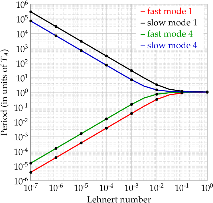
Figure 3: Left: Period $T$ (expressed in Alfvén time) as a function of Lehnert number $\mathrm{Le}$ for the first and fourth radial modes, for an azimuthal wavenumber $m=6$, in the same framework as reported in table 2. Right: Period $T$ as a function of azimuthal wavenumber $m$ for a fixed Lehnert number $\mathrm{Le}=10^{-4}$ for the first and fourth radial modes. Lines indicate theoretical periods, as taken from (44) and (45) in which $\lambda$ is also a function of $m$, black dots are calculated using our numerical code

Figure 3 displays the periods of the modes in the exponential container. The left panel shows the dependency of the period on the Lehnert number, for the first and fourth eigenmodes in radius, and for azimuthal wavenumber $m=6$. The results obtained in this global analytical case are in agreement with the asymptotic theory, (48)-(49) above, as the period is proportional to $\mathrm{Le}$ on the fast branch and to $\mathrm{Le}^{-1}$ on the slow branch. The right panel represents the dependency of the period on $m$ at $\mathrm{Le}=10^{-4}$, for the same eigenmodes. The periods seem to scale with $1/m$; this corresponds roughly to the zeros of the determinant $\mathcal{D}(\eta)$ since $m$ appears in the degree of the Bessel functions defining the determinant $\mathcal{D}$.

The value of the above simple solution is that it provides exact values for $\lambda$ in (42), which in turn allows the corresponding frequencies of the global modes to be exactly determined. The corresponding modes furthermore possess a precise analytic form, depending in a relatively simple fashion on $\beta$. These known eigenvalues and eigenfunctions provided us with a benchmark case that enabled us to validate the numerical method described in section 2 that was used in the following sections to compute catalogs of eigenmodes and eigenfrequencies for more general configurations of the boundary slope and the background zonal magnetic field.

4 Numerical results

4.1 Influence of container geometry: the hydrodynamic case

We begin by numerically investigating the influence of the shape of the container on the spatial structure of the modes. We compare the exponential container (also discussed in section 3, corresponding to a constant $\beta=-1$), a sloped cylinder (corresponding to a constant slope $H^{\prime}(s)=-1$), and a spherical shell all of inner radius $r_{i}=0.35$ and outer radius $r_{o}=1$. To simplify the comparison, we restrict the study to hydrodynamic Rossby modes defined by

$$\left[\omega\left(\frac{1}{s}\partial_{s}s\partial_{s}-\frac{m^{2}}{s^{2}}-\beta\partial_{s}\right)+2\frac{m\beta}{s}\right]\hat{\Psi}=0.$$ (58)

Since the Alfvén time scale is meaningless in this non-magnetic context, time has here been scaled by the rotation time scale $\Omega^{-1}$ and velocities with $r_{o}\Omega$. As in the hydromagnetic study, the information concerning the meridional shape of the axisymmetric container is contained in the $\beta$ parameter (first defined in Eq. (16)).

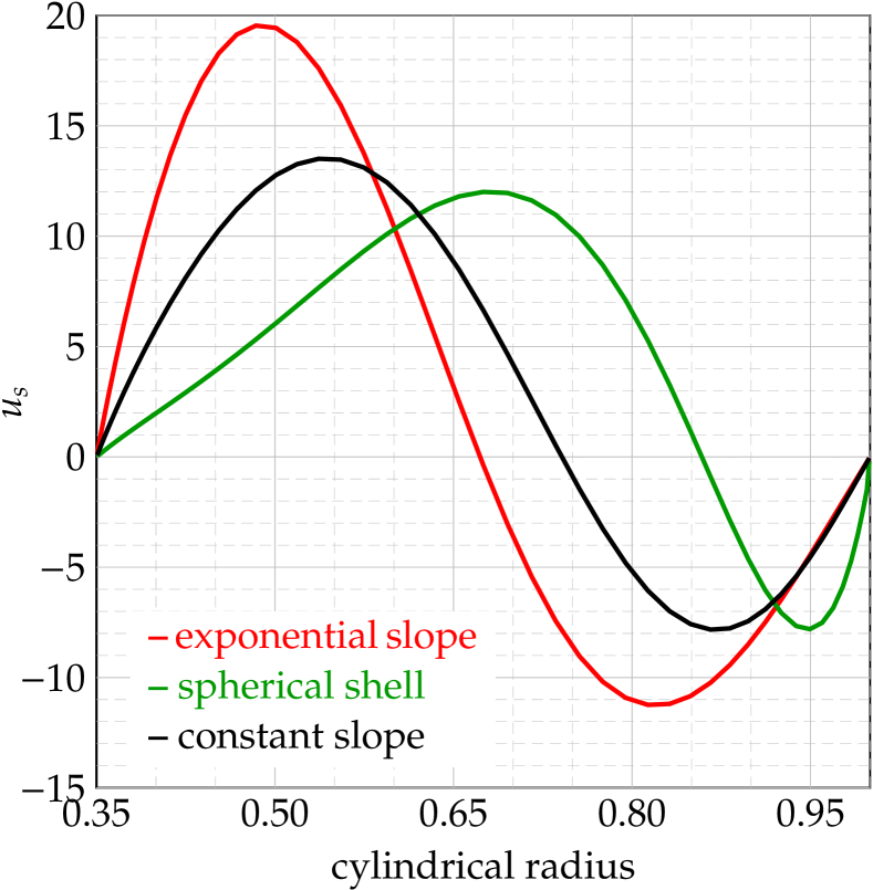
Figure 4: Influence of the shape of the container on the radial velocity ($u_{s}$) profile of the second eigenmode of azimuthal wavenumber $m=6$ as a function of the cylindrical radius $s$. Black curve: sloped container (constant slope $H^{\prime}(s)=-1$), red curve: exponential container (constant $\beta=-1$), green curve: spherical container

Figure 4 displays radial velocity profiles corresponding to the second eigenmodes in radius for the azimuthal wavenumber $m=6$, as a function of the cylindrical radius for three different containers. For the spherical shell and the constant-slope annulus, $\beta$ and thus the restoring force depend on $s$; the restoring force is stronger further away from the inner boundary – since (i) the slope is larger (in the spherical case), or (ii) the column height is smaller (in the annulus) near the outer boundary – leading to a smaller node spacing in the vicinity of the outer boundary. For example, for the sixth eigenmode in a sphere, the non-dimensional distance between two nodes near the tangent cylinder is 0.2 whereas it drops to 0.03 near the outer boundary. This results in the eigenfunction effectively being concentrated towards the outer boundary.

The shape of the container therefore clearly does influence the form of global QG modes, and a simple constant $\beta$ theory cannot capture the full nature of modes in a spherical shell. Another question of interest, in the spherical case, is the relevance of the QG approximation for accurately capturing global, fully three-dimensional inertial modes. We address this question in detail in A. In a nutshell, we find a remarkable agreement (in terms of the spectra predicted) when longest periods modes (with low $m$ and small radial wavenumber) are considered.

4.2 Influence of background zonal magnetic field

These initial findings encourage us to return to the (more complete) hydromagnetic problem defined by Eqs. (37) and (38), considering for now only the diffusionless scenario. We numerically find solutions to the eigenvalue problem (40), obtaining both flow and field eigenfunctions and their corresponding eigenfrequencies. We explore the influence of different background zonal field profiles defined in (29) - (32) on the dispersion relation and spatial structure of the QG hydromagnetic modes in the spherical shell geometry most relevant for planetary cores. Figure 5 displays the periods for the fast and slow modes as a function of $\mathrm{Le}$ (Left panels, with $m=6$) and a function of the azimuthal wavenumber $m$ (Right panels, with $\mathrm{Le}=10^{-4}$) for the four different background magnetic fields. The upper and lower panels corresponds to the radial structure of the mode, namely the first (upper) and fourth (lower) modes in radius.

The background magnetic field structure does not influence the scaling of the mode period with respect to $\mathrm{Le}$ and $m$. The scalings found here numerically for the slow waves are in agreement with the asymptotic theory presented earlier (see Eqs. (48) and  (49)). The fast mode, essentially a Rossby mode, is not sensitive to the background magnetic field for $\mathrm{Le}<10^{-2}$. Its period is proportional to $\mathrm{Le}$ and depends only weakly on the azimuthal wavenumber.

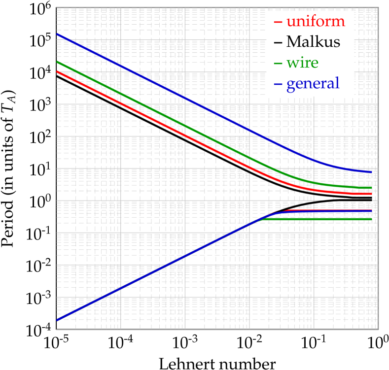
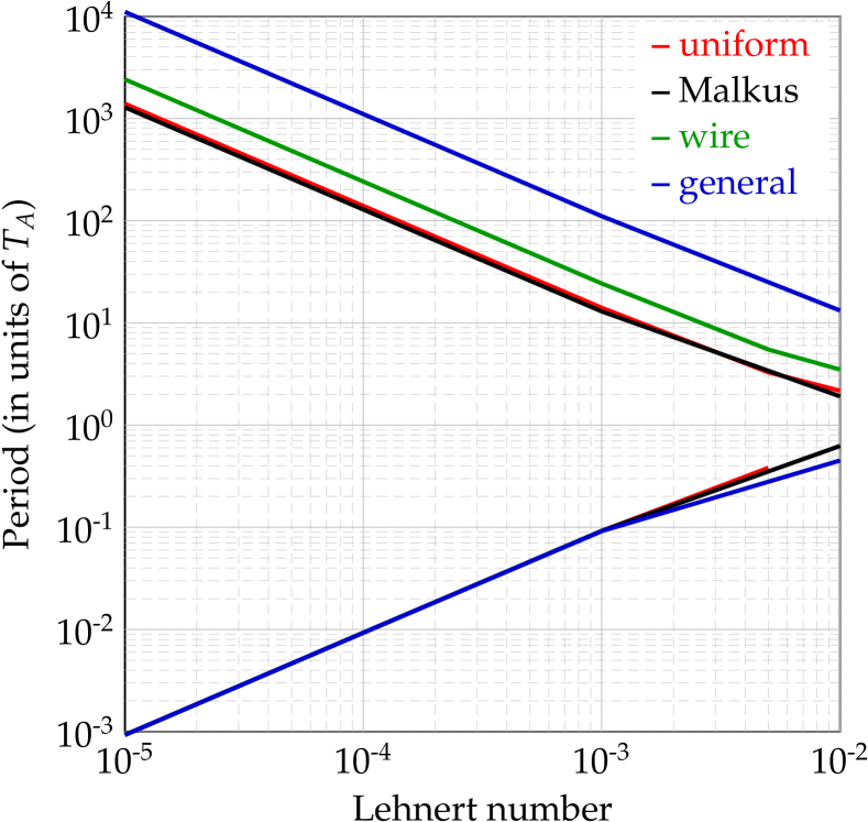
Fundamental mode
$m=6$ $\mathrm{Le}=10^{-4}$
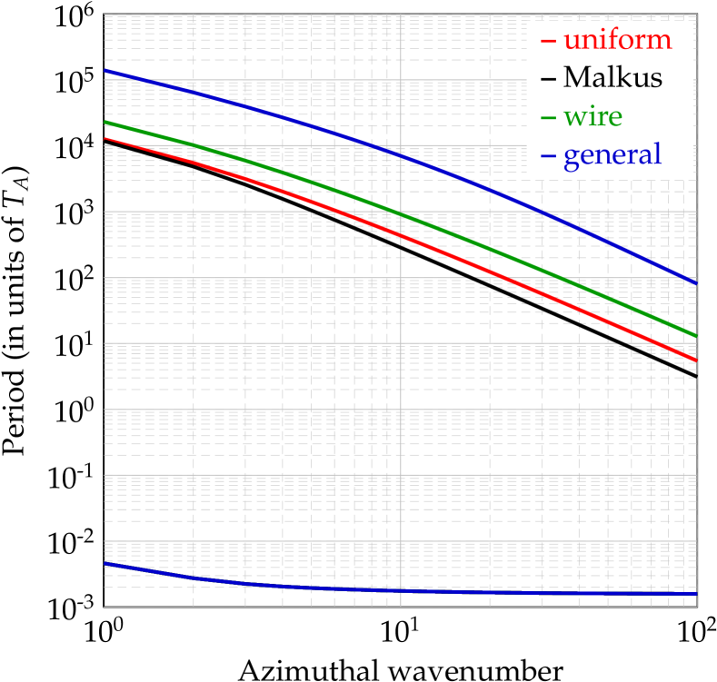
Third overtone
$m=6$ $\mathrm{Le}=10^{-4}$

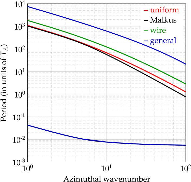
Figure 5: Periods of the fast and slow QG modes for varying Lehnert number, azimuthal wavenumber, and background magnetic field. The top row corresponds to the fast and slow fundamental modes, and the bottom row to the fast and slow third overtones (fourth modes in the catalog). The periods shown in the left column are those of modes having azimuthal wavenumber $m=6$ (with varying Lehnert number and background field). Those shown in the right column have fixed Lehnert number ($\mathrm{Le}=10^{-4}$), and varying wavenumber and background field. The effect of four different background zonal magnetic fields is also presented: uniform field (red curves), Malkus field (black curves), field due to a wire at the axis of rotation (green curves) and a more general zonal field (blue curves). Note that for the fast modes curves due to different fields overlap.

In the limit of rapid rotation ($\mathrm{Le}<10^{-2}$), the period of the slow mode scales as the inverse of $\mathrm{Le}$ but with the modes due to different zonal background fields offset from one another. The relation between the spatial structure of the background field and the exact period of the slow waves is not straigthforward. For example, the non-monotonic zonal field (labelled general) is the most complicated in space, involving large spatial gradients but the global analysis, perhaps surprisingly, shows that in this case, modes with longer periods are in fact produced, with the modes being concentrated near the outer boundary where the magnetic field is weakest (see Fig. 6). The restoring Lorentz force most relevant to the eigenmodes arises due to the gradients generated by the time-varying, disturbance magnetic field. Because the general background field is weakest at large s, and lower than any other choice of background field considered, the eigenfunctions can condense into that region resulting in a longer period for the modes.

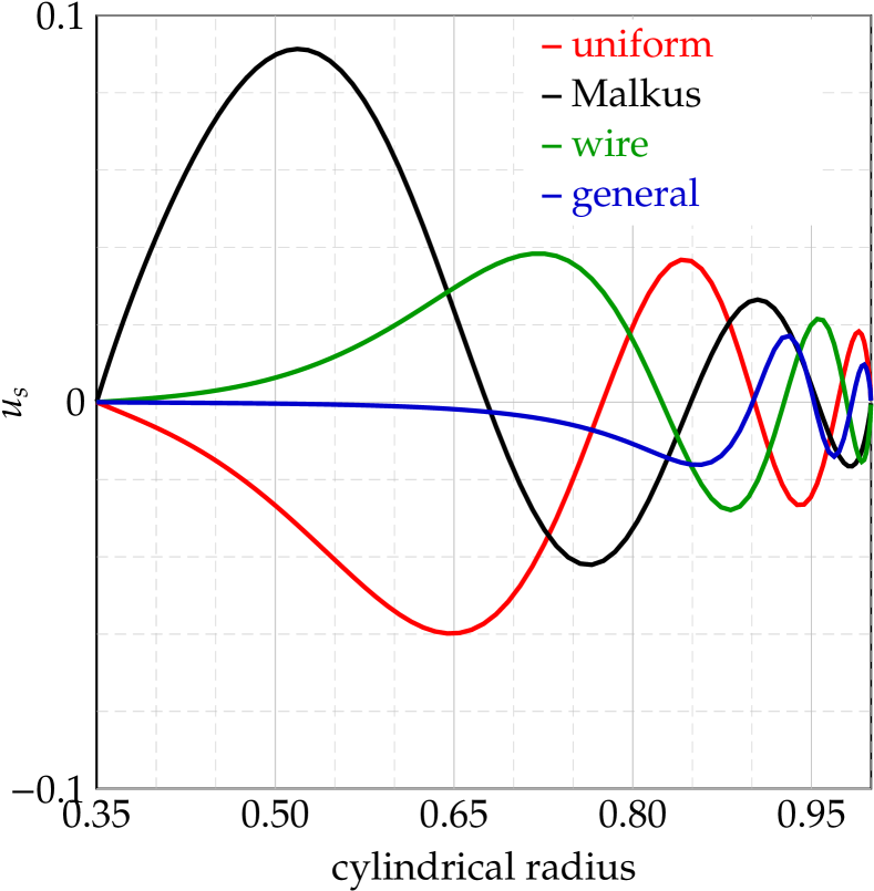
Figure 6: Profile of the radial velocity $u_{s}$ for the slow magnetic modes (4th modes (third overtones) in radius, $m=6$) for the four background magnetic fields described in the text: uniform field (red curve), Malkus field (black curve), field due to a wire current at the axis of rotation (green curve) and a more general zonal field (blue curve).

4.3 Influence of Ohmic dissipation

As described above, the slow modes are essentially magnetic, while the fast modes are essentially hydrodynamic and only weakly feel the magnetic field. When magnetic dissipation is included, local theory for plane hydromagnetic waves (e.g. Rüdiger and Hollerbach, 2004, section 2.5) suggests that the fast wave, which is essentially of inertial type, is not affected by magnetic dissipation, whereas the slow one is essentially forced to decay. How the structure of the mode is affected by magnetic diffusion is not addressed by the local theory. Here, we solve problem (40) in spherical shell geometry, in the presence of the general zonal background magnetic field, and including magnetic dissipation whose level is controlled by the Lundquist number as defined in (2).

$\Psi$, $\mathrm{Lu}=+\infty$, slow mode

$\Psi$, $\mathrm{Lu}=+\infty$, fast mode

$\Psi$, $\mathrm{Lu}=10^{4}$, slow mode

$\Psi$, $\mathrm{Lu}=10^{4}$, fast mode

$\Psi$, $\mathrm{Lu}=10^{2}$, slow mode

$\Psi$, $\mathrm{Lu}=10^{2}$, fast mode

Figure 7: Contours of the velocity streamfuction $\Psi$ in the equatorial plane as seen from above. Shape of the fundamental eigenfunction of azimuthal wavenumber $m=6$ for the slow mode (left panels) and the fast mode (right panels) in spherical shell geometry in the presence of the general background field. The first row corresponds to no magnetic dissipation whereas the second and third rows are for $\mathrm{Lu}=10^{4}$ and $\mathrm{Lu}=10^{2}$ respectively. All figures are $Le=10^{-4}$. All streamfunctions are normalized, and the plots show ten equally-spaced levels in positive (solid contours) and negative (dashed contours). The thick black line shows the background magnetic field profile.

$A$, $\mathrm{Lu}=+\infty$, slow mode

$A$, $\mathrm{Lu}=+\infty$, fast mode

$A$, $\mathrm{Lu}=10^{4}$, slow mode

$A$, $\mathrm{Lu}=10^{4}$, fast mode

$A$, $\mathrm{Lu}=10^{2}$, slow mode

$A$, $\mathrm{Lu}=10^{2}$, fast mode

Figure 8: Contours of the magnetic streamfuction $A$ in the equatorial plane as seen from above. Shape of the fundamental eigenfunction of azimuthal wavenumber $m=6$ for the slow mode (left panels) and the fast mode (right panels) in spherical shell geometry in the presence of the general background field. The first row corresponds to no magnetic dissipation whereas the second and third rows are for $\mathrm{Lu}=10^{4}$ and $\mathrm{Lu}=10^{2}$ respectively. All figures are for $\mathrm{Le}=10^{-4}$. All streamfunctions are normalized, and the plots show ten equally-spaced levels in positive (solid contours) and negative (dashed contours). The thick black line shows the background magnetic field profile.

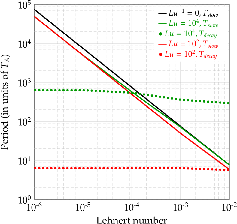
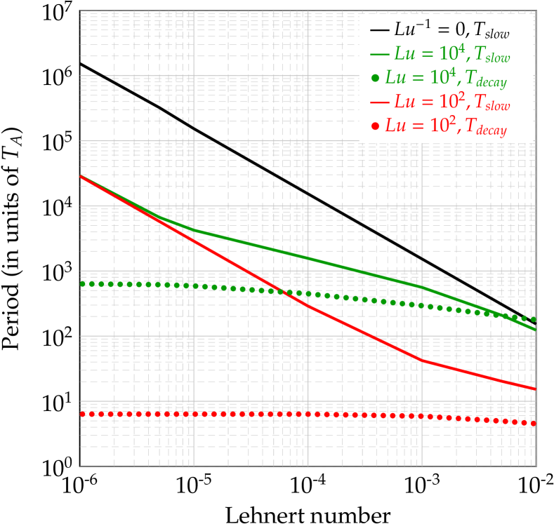
Figure 9: Oscillation (pseudo) periods and decay times for the modes as a function of $\mathrm{Le}$, for the fundamental mode in radius with azimuthal wavenumber $m=6$. Black solid curves for modes without dissipation $\mathrm{Lu}=+\infty$, Green curves for weak magnetic dissipation $\mathrm{Lu}=10^{4}$ (solid: period, bullets: decay time), blue curves for strong magnetic dissipation $\mathrm{Lu}=10^{2}$ (solid: period, bullets: decay time). The background field is the Malkus field (left panel) and the more general zonal field (right panel) respectively.

Figure 7 presents contours of the velocity stream function in the equatorial plane for the slow (left panels) and fast (right panels) fundamental hydromagnetic modes for azimuthal wavenumber $m=6$ with various amount of magnetic dissipation present. The upper panels show the diffusionless case ($\mathrm{Lu}=+\infty$), while the middle and lower panels involve $\mathrm{Lu}=10^{4}$ and $\mathrm{Lu}=10^{2}$ respectively. The basic structure of the fast modes is essentially unchanged by the introduction of magnetic dissipation although the velocity streamfunctions do show a small phase shift that depends on the amount of dissipation but is independent of the background magnetic field. The structure of the slow mode, on the other hand, is strongly influenced by the dissipation. At $\mathrm{Lu}=10^{4}$, the velocity field spirals as a function of cylindrical radius, while if dissipation is increased further up to $\mathrm{Lu}=10^{2}$ it becomes straight again but now shifted toward the inner core suggesting another mechanism then controls the mode structure.

Figure 8 presents similar plots of the magnetic streamfunction. Note the magnetic and velocity stream functions are now no longer identical, as was the case in the study of Malkus (1967) and for the analytic solutions we presented above, instead the velocity stream functions are now noticeably more compressed towards the core-mantle boundary than the magnetic stream functions. Considering the fast modes, the magnetic and velocity streamfunctions are found to be in anti-phase. Considering the slow modes, the magnetic and velocity streamfunctions are in phase for the diffusionless and weak diffusion cases, but exactly out-of-phase when the magnetic diffusion is strong (Lu=100). In both Figure 7 and Figure 8 the background magnetic field is plotted as the thick black line. It seems to dictate where spiralling of the modes (both in the velocity field and the magnetic field) takes place in the intermediate regime of weak magnetic diffusion. In particular, with the general zonal background field investigated here, the spiraling pattern is narrow and located where the gradient of the background field is large. With the Malkus background magnetic field the spirals are broader and fill the whole domain (not shown).

Figure 9 documents the influence of magnetic dissipation ($\mathrm{Lu}=10^{2},10^{4}$) or no dissipation on mode periods for the case of the Malkus (left panel) and more general (right panel) background zonal magnetic fields. The crucial change compared to the diffusionless case is that the eigenfrequency becomes complex. The real part of the eigenfrequency then defines the pseudo-period or oscillations period of the mode, for example,

$$T_{slow}=\frac{2\pi}{\mathrm{Re}\left\{\omega\right\}}$$ (59)

while the imaginary part of the eigenfrequency corresponds to its decay time

$$T_{decay}=\frac{2\pi}{\mathrm{Im}\left\{\omega\right\}}.$$ (60)

In both panels, there are regions of parameter space where the decay timescale $T_{decay}$ is comparable to, or shorter than, the pseudo-period $T_{slow}$. In such cases, the mode will have no time to oscillate before it is dissipated.

5 Discussion

A fundamental assumption in this study is that the axially invariant QG model is an adequate description of transient flow disturbances on time scales slower than the rotation time scale. Detailed comparisons with slow (three-dimensional) inertial waves in a sphere (see A) suggest that this is indeed the case in the hydrodynamic scenario, provided that one considers large scale (low $m$) motions that are slow enough for inertia to be negligible. In the hydromagnetic case, a further requirement is that the Lorentz force should remain much weaker than the the Coriolis force. At the very low Lehnert numbers of $10^{-3}-10^{-6}$ relevant for planetary cores this is the case, even if the background magnetic field is fully three dimensional (Gillet et al., 2011). A more troublesome assumption is that the magnetic field perturbation is also axially invariant. This is likely reasonable in the diffusionless limit, and probably also when magnetic diffusion is weak, but when magnetic diffusion is strong it will certainly break down. In the quasi-free decay regime (which is likely of limited dynamical relevance because the decay time scale of these modes is shorter than their oscillation time scale) full three-dimensional models such as described by Schmitt (2012) should be preferred to a QG approach.

Interestingly, the QG model implemented here is not restricted to a spherical shell, but can be used to study any axisymmetric container. This allows comparisons to be made with earlier annulus type models with constant boundary slope. The spherical shell geometry appropriate for planetary cores, with the boundary slope increasing as a function of the cylindrical radius, causes eigenfunctions to become more compressed towards the outer boundary at large cylindrical radius, particularly when higher radial overtones are considered. If the background magnetic field also varies with cylindrical radius, this provides an additional modulation of the radial structure of the modes. As illustrated in Figure 6, the mode amplitude tends to be enhanced where the magnetic field is weaker. Since in planetary cores the toroidal field is expected to decay towards the outer boundary (since silicate mantles are relatively poor electrical conductors) this will also tend to push the mode minima and maxima out to large cylindrical radius. A prediction of our QG model of hydromagnetic modes in a spherical shell is therefore that the free oscillation modes are more likely to be observed at mid to low latitudes.

Perhaps the most important finding of this study is that magnetic dissipation will strongly influence the properties of slow magnetic modes in planetary cores. In our numerical experiments a transition from diffusionless slow modes to slow modes dominated by diffusion (referred to as quasi free decay (QFD) modes by Schmitt (2012)) occurs as the Lehnert number becomes smaller than the inverse Lundquist number. For lower Lehnert numbers, the decay time of the slow modes is much shorter than their oscillation time, so they will rapidly decay and are precluded from playing an important role in the core dynamics or producing observable secular variation. The transition from diffusionless to QFD slow magnetic modes happens at higher Lehnert number when the background magnetic field is more complex in the radial direction. Since $\mathrm{Le}\cdot\mathrm{Lu}=\mathrm{\Lambda}$ is the traditional Elsasser number, another way to state this is that for $\mathrm{\Lambda}\ll 1$, free slow magnetic modes are expected to rapidly decay. This conclusion was essentially arrived at previously by Schmitt (2012) in his study of a small number of 3D modes, here we confirm this finding for our more extensive catalogue of QG modes.

	$m$	$m=3$			$m=6$			$m=12$
	radial mode	1	2	4	1	2	4	1	2	4
Malkus	$T_{slow}$ (yrs)	$10300$	$3100$	$1244$	$3080$	$1310$	$529$	$833$	$380$	$171$
	$T_{decay}$ (yrs)	$41750$	$13900$	$4013$	$15500$	$6800$	$2707$	$4800$	$2400$	$1212$
General	$T_{slow}$ (yrs)	$43800$	$7600$	$1840$	$24000$	$5000$	$1260$	$11100$	$2900$	$794$
	$T_{decay}$ (yrs)	$24000$	$5300$	$1478$	$12600$	$3400$	$969$	$5700$	$2000$	$627$

Table 3: Pseudo-period $T_{slow}=\frac{2\pi}{\mathrm{Re}(\omega)}$ and decay time $T_{decay}=\frac{2\pi}{\mathrm{Im}(\omega)}$ in years for Earth’s core (taking $\mathrm{Le}=10^{-4}$ and $\mathrm{Lu}=10^{5}$, a value representative of the range estimated for Earth’s core $\left[59,000-186,000\right]$ assuming the core interior field strength of $3$ mT proposed by Gillet et al. (2010)). Results for slow QG modes with azimuthal wave numbers $m=3,6,12$ and three radial modes (the 1st, 2nd and 4th modes) are presented. Results are shown for both the Malkus general field and the more realistic general zonal field. To obtain these times in years, the non-dimensional results from the numerical model were rescaled using $1T_{A}=4.51$ years, as is appropriate for $\mathrm{Le}=10^{-4}$.

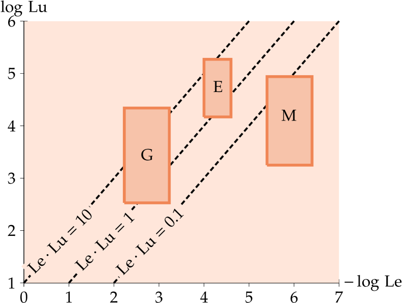
Figure 10: Approximate location of Earth (E), Ganymede (G) and Mercury (M) in the $\mathrm{Le}-\mathrm{Lu}$ plane (logarithmic scales). The estimates come from the data presented in table 1.

For the Earth’s core we estimate the Lehnert number lies in the range $\mathrm{Le}=\left[2.5\cdot 10^{-5}-10^{-4}\right]$ while the Lundquist number is estimated to lie in a range $\left[14,750-186,000\right]$ so the Elsasser number is in the range $\left[0.4-18.6\right]$ (see Table 1). It is therefore possible that a transient slow hydromagnetic mode might be observed for a few periods before it decays, especially if the strong field proposed by Gillet et al. (2010) and the most recent values for core conductivities (de Koker et al., 2012; Pozzo et al., 2012), which lead to the upper estimates of $\mathrm{Le}$ and $\mathrm{Lu}$, prove to be correct. However, this will also depend on the complexity of the background magnetic field. This point is demonstrated in Table 3 where the pseudo-periods and decay times in years, rescaled using parameters appropriate for the Earth’s core, are presented for the Malkus background field and the general zonal background field. For the Malkus background field, we find decay times longer than the oscillation times while for the general zonal background field the opposite is true. The decay time approaches the oscillation time for higher overtones, so these may still be of observational relevance. It is the low Lehnert number in planetary cores that ensures the slow modes have a magnetic energy much larger than their kinetic energy - see (51). This underlies the important role played by magnetic diffusion for the slow modes. The opposite is true for the fast modes which have kinetic energy much larger than their magnetic energy. An additional source of dissipation that may be important in planetary cores, but which has for simplicity been neglected here, is boundary coupling. For example, if the lowermost mantle involves a layer with high electrical conductivity then the magnetic field will penetrate into it and the differential motion between the core fluid and the mantle will shear the magnetic field dissipating energy. Dumberry and Mound (2008) investigate this source of damping in a study of torsional oscillations. Consideration of this mechanism would require a modification of our simple boundary conditions, and may further shorten the decay time scale for the slow magnetic modes.

It is noticeable that the periods of the large-scale slow magnetic modes obtained using the general zonal background field (see table 3) are rather longer than the time scales of order 300 years normally associated with westward drifting flux patches at Earth’s core surface. Furthermore, in his pioneering study, Hide (1966) highlighted somewhat shorter periods for the slow magnetic modes. We find that the periods of the slow magnetic modes are very sensitive to both the shape and the strength of the background magnetic field, for example, even in the simplest case the dimensional period of the slow mode scales as $B_{0}^{2}$ (in (49), units of $T_{A}$ are used), so a change in the field strength by only a factor of 3 would result in an order of magnitude change in the mode period. For our specific choice of background field structure and strength (see table 3) some westward bulk advection would be necessary in addition to the QG modes in order to explain the observed rate of westward drift. More accurate conclusions must await an improved knowledge of the background magnetic field in Earth’s core. It has not escaped our attention that this sensitivity of mode structure to the background magnetic field may provide a means of probing (inverting) for magnetic field structure within Earth’s core.

Figure 10 presents the location of Earth, Ganymede and Mercury in a $\mathrm{Le}-\mathrm{Lu}$ plane, about a $\mathrm{\Lambda}=1$ straight line. Our results imply that free oscillation, slow, magnetic modes will be rapidly damped by magnetic dissipation in the core of Mercury, while in Earth and possibly Ganymede QG modes modified by diffusion may persist for a few periods before decaying. The fast modes, on the other hand are only weakly influenced by magnetic dissipation and are expected to be present in all the planetary cores considered. If hydromagnetic modes were continuously or intermittently forced in the cores of Earth or Ganymede they could play an important role in transient dynamics, particularly if the Elsasser number for these bodies turns out to be at the larger end of current estimates. It will nonetheless be a major observational challenge to conclusively observe these hydromagnetic modes. One requires globally distributed magnetic observations for a time scale comparable to their period. For the slow magnetic modes, this is hard to envisage except perhaps for the Earth. But for the fast modes observational identification using magnetic measurements from orbital satellites may be mor feasible, provided mantle conductivities of the planets are not so large as to filter out the mode signatures, and provided the external (non-core) magnetic field fluctuations can be efficiently separated at the periods of the modes.

In an effort to focus on the intrinsic properties of QG modes, no excitation source was included in our model. The logic of first establishing the properties of the free oscillations and then using them within a Green’s function framework, with a particular excitation source, is well known from normal mode seismology and more recently from study of torsional oscillations in Earth’s core (Buffett et al., 2009). A similar development could be envisaged for the non-axisymmetric hydromagnetic QG modes discussed here, although their non-normal nature should be borne in mind. What are the possible excitation sources? Most obviously there is thermochemical core convection. The time scales of several hundred years for convective overturn in the Earth’s core are appropriate for exciting axially invariant motions and QG hydromagnetic modes. Other possibilities include shear flow instability or instability of magnetic field itself. A final intriguing possibility is topographic forcing along the lines originally proposed by Hide (1966). The time scale and spatial structure of the forcing mechanisms (e.g. fluctuations in columnar convection outside the tangent cylinder, shear instability near the tangent cylinder, or magnetic field instability at low latitudes close to the outer boundary where the shear in the toroidal field may be large) will determine which modes are preferentially excited and possibly maintained against diffusion long enough to be observed.

Linear models of waves and modes, such as that presented here, have proven important in obtaining physical insight in other geophysical and planetary scale fluid systems, including Earth’s atmosphere and oceans. But to explain geophysical observations in detail it is usually necessary to go beyond such simple linear models, and to consider not only excitation sources but also coupling, feedback and saturation between the mean state and the disturbances. The linear model presented here is not suitable for such studies, these require fully nonlinear QG models of core dynamics that are currently under development. Indeed the long periods obtained for the slow magnetic modes in this study lead us to expect that the background magnetic field will evolve on a time scale similar to that of the slow modes. Nonlinear models are thus essential for an assessment of the physical relevance of the slow magnetic modes. Such nonlinear models will more generally enable us to answer important questions such as whether transient hydromagnetic modes riding apon large-scale gyres (generated by convection in planetary cores), could have an observable imprint on the magnetic field variations of these bodies.

Appendix A Comparison between quasi-geostrophic modes and slow inertial modes in a sphere

In this appendix, we present a comparison between free oscillations predicted by our QG model with a spherical outer boundary, and previously derived analytical solutions for slow inertial modes in a full sphere (Zhang et al., 2001). The later solutions involve no a priori assumption of quasi-geostrophy (i.e. no axial averaging). This comparison is an interesting test of our QG model, providing a quantitative benchmark against known solutions, and allow us to ascertain the conditions under which the QG approximation breaks down.

It has long been recognized that Rossby modes in a closed container are no more than a special class of inertial modes, in which ${\partial{\bf u}/\partial t}$ is much smaller than the pressure and Coriolis forces, so that related motions are very close to geostrophic (Longuet-Higgins, 1964; Greenspan, 1968; Busse et al., 2005). Although we present a comparison here of purely hydrodynamic modes, it is interesting to note that in the case of an imposed Malkus magnetic field (30), then a very similar comparison can also be made for hydromagnetic modes – see Malkus (1967); Zhang et al. (2003).

Since the comparison in this section relies on the inertial mode solutions of Zhang et al. (2001), we briefly remind the reader of their salient characteristics.

The inertial modes in a sphere are the solutions to

$$\partial_{t}\mathbf{u}+2\boldsymbol{e}_{z}\times\mathbf{u}=-\boldsymbol{\nabla}p$$ (61)

and

$$\boldsymbol{\nabla}\cdot\mathbf{u}=0,$$ (62)

subject to the impenetrable boundary condition $u_{r}=0$ on the the spherical surface at $r=r_{o}$. To facilitate comparisons with Zhang et al. (2001), the rotation time scale $\Omega^{-1}$ has been used here to non-dimensionalize. Expanding these vector equations into cylindrical co-ordinates, considering solutions of the form

$$\mathbf{u}(s,\varphi,z)=\left[U_{s}(s,z),U_{\varphi}(s,z),U_{z}(s,z)\right]e^{\mathrm{i}(m\varphi+2\sigma t)},$$ (63)

and substituting between the components to eliminate pressure, Zhang et al. (2001) show how the half frequencies $\sigma$ for equatorial symmetric solutions i.e. for which $(U_{s},U_{\varphi},U_{z})(\cdot,z)=(U_{s},U_{\varphi},-U_{z})(\cdot,-z)$ (the symmetry compatible with the QG model) can be found from the roots of the equation

$$\sum^{N}_{j=0}(-1)^{j}\frac{[2(2N+m-j)]!}{j!(2N+m-j)![2(N-j)]!}\left[(m+2N-2j)-\frac{2(N-j)}{\sigma_{Nmn}}\right]\sigma_{Nmn}^{2(N-j)}=0.$$ (64)

Different solutions are obtained for $N=0,1,2,\dots$ and $n$ indexes the possible modes for a given choice of $N$ and $m$. Zhang et al. (2001) describe how in the triplet $\left\{Nmn\right\}$, $m$ denotes the azimuthal wavenumber, $N$ defines the degree of possible complexity in the axial ($z$) direction and $n$ is related to the cylindrical radial structure.

Considering the special case of slow inertial modes for which

$$\sigma_{si}=\sigma_{Nmn}\ll\mathcal{O}(m/(N+m),$$ (65)

that are close to geostrophy and so possess relatively simple structures in the axial $z$ direction, then an analytic approximation to (64) is available (Zhang et al., 2001; Busse et al., 2005)

$$\omega_{si}\simeq-{2\over m+2}\left[\sqrt{1+\frac{m(m+2)}{N(2N+2m+1)}}-1\right],$$ (66)

where $\omega_{si}=2\sigma_{Nmn}$ and this approximation is exact for the case $N=1$. All such slow modes propagate eastwards and are none other than the well known Rossby modes in a full sphere(Busse et al., 2005).

Here, we compare the mode frequencies determined from the Zhang et al. (2001) theory (64) with those computed numerically using our QG model in the absence of any magnetic field, with spherical boundaries and with a vanishingly small inner core (tests showed that provided this is chosen sufficiently small, the inner core has a negligible effect on the modes discussed here). In this case our QG model reduces to (58) :

$$\left[\omega_{qg}\left(\frac{1}{s}\partial_{s}s\partial_{s}-\frac{m^{2}}{s^{2}}-\beta\partial_{s}\right)+2\frac{m\beta}{s}\right]\hat{\Psi}=0,$$ (67)

where, as before, $\beta(s)=H^{\prime}(s)/H(s)$ and we impose the boundary conditions $\Psi=0$ at $s=1$ and $s=0.01$. As previously, we expand $\hat{\Psi}$ as a sum of Chebyshev polynomials and impose the equations and boundary conditions using a collocation method. In this scenario a rather simple real, linear, algebraic eigenvalue problem in $\omega_{qg}$ is obtained. Results for both $\omega_{si}$ and $\omega_{qg}$ are presented for comparison in Figure 11, as a function of the azimuthal wavenumber $m$ for five example radial modes.

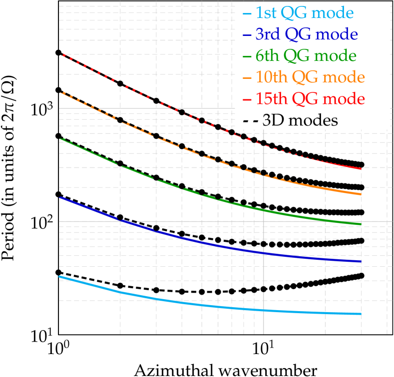
Figure 11: Periods (in units of $2\pi/\Omega$) of hydrodynamic QG modes in a sphere as a function of azimuthal wavenumber. The coloured lines show the results for quasi-geostrophic modes of increasing complexity (smaller wavelength) in the radial direction. The corresponding predictions from the Zhang et al. (2001) theory are shown as dashed-bulleted lines.

For the longest period (slowest) modes (with low $m$ but high radial wavenumber) the agreement between the QG numerical model and the predictions of the Zhang et al. (2001) analytic theory is excellent. This is encouraging since it shows that when the flow disturbances are very close to geostrophic then the QG model performs as desired, giving good agreement with full three-dimensional solutions. We can also see that for azimuthal wave numbers below $m=10$ the QG model generally performs rather well, especially for disturbances with short wavelength in the radial direction.

Nonetheless, there is evidently a poor agreement between our QG model and the three-dimensional theory for the modes with largest radial wavelengths, particularly when the azimuthal wavenumber is very high. Examination of the associated eigenfunctions shows that, for a given radial mode, as $m$ increases the eigenfunction is increasingly pushed towards the outer boundary; in this region the boundary slope is large and the three-dimensional solutions show more prominent departures from axial invariance that are incompatible with the QG assumption, compare for example Figures 1 and 2 from Busse et al. (2005) for $m=6$. The failure of the QG model manifests itself in terms of an incorrect slope of the dispersion curve at very large $m$, see for example the mode with larges radial length scale (the blue curve in Figure 11); physically this implies that the azimuthal group velocity of such modes is incorrect in the QG model.

We note here in passing that we have presented results from a quasi-geostrophic formulation that includes three-dimensional mass conservation, rather the simpler small-slope approximation that was imposed in early models (Schaeffer and Cardin, 2005; Canet et al., 2009). The agreement between the QG model predictions including three-dimensional mass conservation and the Zhang et al. (2001) modes was found to be superior than that for a formulation based on the small-slope approximation.

The results presented here provide evidence that our QG model is a useful tool for study the dynamics of Earth’s core, provided most of the flow energy lies at small azimuth wavenumber, and especially if structures also possess short length scales in the cylindrical radial direction.

References

- Acheson (1972) Acheson, D. J., 1972. On hydromagnetic stability of a rotating fluid annulus. J. Fluid Mech. 52, 529–541.
- Alfvén (1942) Alfvén, H., 1942. Existence of EM-hydrodynamic waves. Nature 150, 405–406.
- Anderson et al. (2008) Anderson, B. J., Acuña, M. H., Korth, H., Purucker, M. E., Johnson, C. L., Slavin, J. A., Solomon, S. C., McNutt, R. L., 2008. The structure of Mercury’s magnetic field from MESSENGER’s first flyby. Science 321 (5885), 82–85.
- Anderson et al. (2012) Anderson, B. J., Johnson, C. L., Korth, H., Winslow, R. M., Borovsky, J. E., Purucker, M. E., Slavin, J. A., Solomon, S. C., Zuber, M. T., McNutt, R. L., 2012. Low-degree structure in Mercury’s planetary magnetic field. J. Geophys. Res. 117, E00L12.
- Braginsky (1964) Braginsky, S. I., 1964. Magnetohydrodynamics of the Earth’s core. Geomagnetism and Aeronomy 4, 698–712.
- Buffett et al. (2009) Buffett, B. A., Mound, J., Jackson, A., 2009. Inversion of torsional oscillations for the structure and dynamics of earth’s core. Geophys. J. Int. 177, 878–890.
- Busse (1970) Busse, F. H., 1970. Thermal instabilities in rapidly rotating systems. J. Fluid Mech. 44, 441–460.
- Busse (1976) Busse, F. H., 1976. Generation of planetary magnetism by convection. Phys. Earth Planet. Int. 12, 350–358.
- Busse et al. (2005) Busse, F. H., Zhang, K., Liao, X., 2005. On slow inertial waves in the solar convection zone. Astr. J. 631, L171–L174.
- Canet et al. (2009) Canet, E., Fournier, A., Jault, D., 2009. Forward and adjoint quasi-geostrophic models of the geomagnetic secular variation. J. Geophys. Res. 114, doi:10.1029/2008JB006189.
- Cébron et al. (2012) Cébron, D., Le Bars, M., Moutou, C., Le Gal, P., 2012. Elliptical instability in terrestrial planets and moons. Astron. Astrophys. 539, 1–16.
- de Koker et al. (2012) de Koker, N., Steinle-Neumann, G., Vlček, V., 2012. Electrical resistivity and thermal conductivity of liquid alloys at high and , and heat flux in Earth’s core. Proc. Natl. Acad. Sci. 109, 4070–4073.
- Deng et al. (2013) Deng, L., Seagle, C., Fei, Y., Shahar, A., 2013. High pressure and temperature electrical resistivity of iron and implications for planetary cores. Geophys. Res. Lett. 40, 33–37.
- Dougherty et al. (2012) Dougherty, M., Grasset, O., Erd, C., Titov, D., Bunce, E., Coustenis, A., Blanc, M., Coates, A., Drossart, P., Fletcher, L., Hussmann, H., Jaumann, R., Krupp, N., Prieto-Ballesteros, O., Tortora, P., Tosi, F., van Hoolst, T., 2012. JUpiter ICy moons Explorer (JUICE): An ESA L-Class Mission Candidate to the Jupiter System. In: Lunar and Planetary Institute Science Conference Abstracts. Vol. 43. p. 1806.
- Dumberry and Mound (2008) Dumberry, M., Mound, J. E., 2008. Constraints on core-mantle electromagnetic coupling from torsional oscillation normal modes. J. Geophys. Res. 113 (B03102).
- Fearn and Proctor (1983) Fearn, D. R., Proctor, M. R. E., 1983. Hydromagnetic waves in a differentially rotating sphere. J. Fluid Mech. 128, 1–20.
- Gillet et al. (2010) Gillet, N., Jault, D., Canet, E., Fournier, A., 2010. Fast torsional waves and strong magnetic field within the Earth’s core. Nature 465, 74–77.
- Gillet and Jones (2006) Gillet, N., Jones, C., 2006. The quasi-geostrophic model for rapidly rotating spherical convection outside the tangent cylinder. J. Fluid Mech. 554, 343–369.
- Gillet et al. (2011) Gillet, N., Schaeffer, N., Jault, D., 2011. Rationale and geophysical evidence for quasi-geostrophic rapid dynamics within the earth’s outer core. Phys. Earth Planet. Int. 187 (3), 380–390.
- Greenspan (1968) Greenspan, H. P., 1968. The theory of rotating fluids. Cambridge University Press.
- Hauck et al. (2006) Hauck, S. A., Aurnou, J. M., Dombard, A. J., 2006. Sulfur’s impact on core evolution and magnetic field generation on ganymede. J. Geophys. Res. 111 (E09008).
- Hauck et al. (2013) Hauck, S. A., Margot, J.-L., Solomon, S. C., Phillips, R. J., Johnson, C. L., Lemoine, F. G., Mazarico, E., McCoy, T. J., Padovan, S., Peale, S. J., Perry, M. E., Smith, D. E., Zuber, M. T., 2013. The curious case of mercury’s internal structure. J. Geophys. Res. 118 (Planets), 1204–1220.
- Hide (1966) Hide, R., 1966. Free hydromagnetic oscillations of the Earth’s core and the theory of geomagnetic secular variation. Phil. Trans. R. Soc. Lond. A 259, 615–647.
- Hulot et al. (2010) Hulot, G., Finlay, C. C., Constable, C. G., Olsen, N., Mandea, M., 2010. The magnetic field of planet Earth. Space Sci. Rev. 152 (1-4), 159–222.
- Jault (2008) Jault, D., 2008. Axial invariance of rapidly varying diffusionless motions in the Earth’s core interior. Phys. Earth Planet. Int. 166, 67–76.
- Jones (2003) Jones, C., 2003. Dynamos in planets. In: Stellar Astrophysical Fluid Dynamics, Edited : M. J. Thompson and J. Christensen-Dalsgaard. Cambridge University Press, pp. 159–176.
- Kivelson et al. (2002) Kivelson, M. G., Khurana, K. K., Volwerk, M., 2002. The permanent and inductive magnetic moments of Ganymede. Icarus 157 (2), 507–522.
- Kono and Roberts (2002) Kono, M., Roberts, P. H., 2002. Recent geodynamo simulations and observations of the geomagnetic field. Rev. Geophys. 40 (4), 1013, doi:10.1029/2000RG00102.
- Lehnert (1954) Lehnert, B., 1954. Magnetohydrodynamic waves under the action of the coriolis force. Astr. J. 119, 647–654.
- Longuet-Higgins (1964) Longuet-Higgins, M. S., 1964. Planetary waves on a rotating sphere. Proc. R. Soc. Lond. A 279, 446–473.
- Malkus (1967) Malkus, W. V. R., 1967. Hydromagnetic planetary waves. J. Fluid Mech. 28, 793–802.
- Nornberg et al. (2010) Nornberg, M., Ji, H., Schartman, E., Roach, A., Goodman, J., 2010. Observation of magnetocoriolis waves in a liquid metal Taylor-Couette Experiment. Phys. Rev. Lett. 104, 074501.
- Olson (2007) Olson, P., 2007. Overview. In: Treatise on Geophysics. Vol. 8: Core Dynamics. ed. Olson, P., Elsevier, Oxford, pp. 1–30.
- Pais and Jault (2008) Pais, A., Jault, D., 2008. Quasi-geostrophic flows responsible for the secular variation of the Earth’s magnetic field. Geophys. J. Int. 173, 421–443.
- Plaut and Busse (2002) Plaut, E., Busse, F., 2002. Low-prandtl-number convection in a rotating cylindrical annulus. J. Fluid Mech. 464, 345–363.
- Pozzo et al. (2012) Pozzo, M., Davies, C., Gubbins, D., Alfè, D., 2012. Thermal and electrical conductivity of iron at Earth’s core conditions. nature 485, 355–358.
- Rüdiger and Hollerbach (2004) Rüdiger, G., Hollerbach, R., 2004. The Magnetic Universe. Wiley-VCH, Ch. 2: Earth and Planets, pp. 3–46.
- Schaeffer and Cardin (2005) Schaeffer, N., Cardin, P., 2005. Quasi-geostrophic model of the instabilities of the Stewartson layer in flat and depth varying containers. Prog. Ocean. 17, 104111.
- Schmitt (2010) Schmitt, D., 2010. Magneto-inertial waves in a rotating sphere. Geophys. Astrophys. Fluid Dyn. 604, 135–151.
- Schmitt (2012) Schmitt, D., 2012. Quasi-free-decay magnetic modes in planetary cores. Geophys. Astrophys. Fluid Dyn. 106, 660–680.
- Schmitt et al. (2008) Schmitt, D., Alboussière, T., Brito, D., Cardin, P., Gagnière, N., Jault, D., Nataf, H.-C., 2008. Rotating spherical Couette flow in a dipolar magnetic field: experimental study of magneto-inertial waves. J. Fluid Mech. 604, 175–197.
- Stevenson (2003) Stevenson, D., 2003. Planetary magnetic fields. Earth Planet. Sci. Lett. 208, 1–11.
- Tobias et al. (2007) Tobias, S., Diamond, P., Hughes, D., 2007. -plane magnetohydrodynamic turbulence in the solar tachocline. The Astrophysical Journal Letters 667 (1), L113.
- Trefethen (2000) Trefethen, L. N., 2000. Spectral methods in MATLAB. Vol. 10. Society for Industrial and Applied Mathematics.
- Wicht et al. (2007) Wicht, J., Mandea, M., Takahashi, F., Christensen, U., Matsushima, M., Langlais, B., 2007. The origin of Mercury’s internal magnetic field. Space Science Reviews 132, 261–290.
- Williams et al. (2010) Williams, P., Read, P., Haine, T., 3 2010. Testing the limits of quasi-geostrophic theory: application to observed laboratory flows outside the quasi-geostrophic regime. J. Fluid Mech. 649, 187–203.
- Yamakawa et al. (2004) Yamakawa, H., Ogawa, H., Kasaba, Y., Hayakawa, H., Mukai, T., Adachi, M., 2004. Current status of the bepicolombo/mmo spacecraft design. Advances in Space Research 33 (12), 2133–2141.
- Zhang (1995) Zhang, K., 1995. Spherical shell rotating convection in the presence of a toroidal magnetic field. Proc. R. Soc. Lond. 448, 245–268.
- Zhang et al. (2001) Zhang, K., Earnshaw, P., Liao, X., Busse, F., 2001. On inertial waves in a rotating fluid sphere. J. Fluid Mech. 437, 103–119.
- Zhang and Fearn (1994) Zhang, K., Fearn, D. R., 1994. Hydromagnetic waves in rapidly rotating spherical shells, generated by magnetic toroidal decay modes. Geophys. Astrophys. Fluid Dyn. 77, 133–157.
- Zhang et al. (2003) Zhang, K., Liao, X., Schubert, G., 2003. Non-axisymmetric instabilities of a torioidal magnetic field in a rotating sphere. Astr. J. 585, 1124–1137.