Hopf fibrations for turbulent pipe flows

Abstract

We propose a generalization of Hopf fibrations to quotient the streamwise translation symmetry of turbulent pipe flows viewed as dynamical systems. In particular, we exploit the geometric structure of the associated high dimensional state space, which is that of a principal fiber bundle. The relation between the comoving frame velocity $U_{d}$ associated with the dynamical phase of an orbit in the bundle and the Taylor’s hypothesis is investigated. As an application, Laser-Induced-Fluorescence techniques are exploited to capture planar fluorescent dye concentration fields tracing a turbulent pipe flow at the bulk Reynolds number $\mathfrak{\mathsf{Re}}=3200$. The symmetry reduction analysis of the experimental data reveals that the speed $u$ of dye concentration bursts is associated with the dynamical and geometric phases of the corresponding orbits in the fiber bundle. In particular, in the symmetry-reduced frame we unveil a pattern-changing dynamics of the passive scalar structures, which explains the observed speed $u\approx U_{d}+U_{g}$ of intense bursting events in terms of the geometric phase velocity $U_{g}\approx 0.43U_{d}$ associated with the orbits in the bundle.

1 Introduction

In the last decade, Navier-Stokes turbulence in channel flows has been studied as a chaotic dynamics in the state space of a high-dimensional system at moderate Reynolds numbers (see, for example, Gibson et al. (2008); Willis et al. (2013)). Here, turbulence is viewed as an effective random walk in state space through a repertoire of invariant solutions of the governing equations (Cvitanović (2013) and references therein). In state space, turbulent trajectories visit the neighbourhoods of equilibria, travelling waves or periodic orbits, switching from one saddle to the other through their stable and unstable manifolds (Cvitanovic & Eckhardt (1991), see also Cvitanović et al. (2013)). Recent studies on the geometry of the state space of Kolmogorov flows (Chandler & Kerswell (2013)) and barotropic atmospheric models (Gritsun (2011, 2013)) give evidence that unstable periodic orbits provide the skeleton underpinning the chaotic dynamics of fluid turbulence.

In pipe flows, the intrinsic continuous streamwise translation symmetry and azimuthal discrete symmetry make difficult identifying invariant flow structures, such as traveling waves or relative equilibria (Faisst & Eckhardt (2003); Wedin & Kerswell (2004)) and relative periodic orbits (Viswanath (2007)), embedded in turbulence. These travel downstream with their own mean velocity and there is no unique comoving frame that can simultaneously reduce all relative periodic orbits to periodic orbits and all travelling waves to equilibria. Recently, this issue has been addressed by Willis et al. (2013) using the method of slices (Siminos & Cvitanović (2011); Froehlich & Cvitanović (2012), see also Rowley & Marsden (2000); Rowley et al. (2003)) to quotient group symmetries and reveal the geometry of the state space of pipe flows at moderate Reynolds numbers. Further, Budanur et al. (2014) exploit the ’first Fourier mode slice’ to reduce the $SO(2)$-symmetry in spatially extended systems. In particular, they separate the dynamics of the Kuramoto-Shivasinsky equation into a ‘shape-changing’ dynamics within a quotient or symmetry-reduced space (base manifold) and a one-dimensional (1-D) transverse space (fiber) associated with the group symmetry. This is the geometric structure of a principal fiber bundle (e.g. Husemöller (1994)), the main topic of our work. In particular, we propose a generalization of Hopf fibrations (Hopf (1931), see also Steenrod (1999)) for dynamical systems with translation symmetries, and apply it to symmetry-reduce the evolution of passive scalars of turbulent pipe flows.

The paper is organized as follows. We first discuss the limitations of the method of comoving frames, also referred to as the method of connections (e.g. Rowley & Marsden (2000)). Then, we provide an overview of principal fiber bundles and present the symmetry reduction scheme via Hopf fibrations. As an application, two-dimensional (2-D) Laser-Induced-Fluorescence (LIF) techniques are exploited to capture planar fluorescent dye concentration fields tracing turbulent pipe flow patterns at Reynolds number $\mathsf{Re}=2U_{b}R/\nu=3200$, where $U_{b}$ is the bulk velocity, $R$ is the radius and $\nu$ is the kinematic viscosity of water. Symmetry reduction of the acquired experimental data is then presented and discussed.

2 Comoving frame velocities and Taylor’s hypothesis

Consider a 2-D passive scalar field $C(x,y,t)$ advected by a velocity field $\mathbf{u}(x,y,t)=(U,V)$ and that evolves according to

$$\partial_{t}C+\mathbf{u}\cdot\nabla C=d\nabla^{2}C+f-s,$$ (2.1)

where $d$ is the diffusion coefficient, $f$ and $s$ are sources and sinks, and ($x,y$) are the horizontal streamwise and vertical cross-stream directions, respectively. The generalization to three-dimensional geometries is straightforward, and it will not be discussed here. Assume that (2.1) admits streamwise translation symmetry, that is if $C(x,y,t)$ is a solution so is $C(x-x_{d},y,t)$ for any drift $x_{d}$. This can be time-varying and related to a comoving frame velocity $U_{d}=\frac{dx_{d}}{dt}$, for which the material derivative

$$\frac{DC}{Dt}=\partial_{t}C+U_{d}\partial_{x}C$$ (2.2)

is, in average, the smallest possible, namely

$$\left\langle\left(\partial_{t}C+U_{d}\partial_{x}C\right)^{2}\right\rangle_{x,y}$$ (2.3)

is minimal if

$$U_{d}(t)=-\frac{\left\langle\partial_{t}C\partial_{x}C\right\rangle_{x,y}}{\left\langle\left(\partial_{x}C\right)^{2}\right\rangle_{x,y}},$$ (2.4)

where the brackets $\left\langle\cdotp\right\rangle{}_{x,y}$ denote space average in $x$ and $y$. In the comoving frame $\left(x-U_{d}t,t\right)$, the passive scalar appears to flow ’calmly’, but still slowly drifting (see, for example, Kreilos et al. (2014) for a study of Couette flows). Only when $\frac{DC}{Dt}=0$, namely diffusion, sources and sinks balance, the flow is steady in the comoving frame (Krogstad et al. (1998)), as for travelling waves (Faisst & Eckhardt (2003); Wedin & Kerswell (2004)). From (2.1), (2.4) can be written as

$$U_{d}(t)=\frac{\left\langle U\left(\partial_{x}C\right)^{2}+V\partial_{x}C\partial_{y}C-(f-s)\partial_{x}C\right\rangle_{x,y}}{\left\langle\left(\partial_{x}C\right)^{2}\right\rangle_{x,y}},$$ (2.5)

which reveals that the comoving frame velocity is a weighted average of the local flow velocities, sources and sinks. Although diffusion processes are invariant under translation, they indirectly affect $U_{d}$ through the concentration gradients. From (2.4), averaging along the $x$ direction only yields the vertical comoving frame velocity profile

$$U_{d}(y,t)=-\frac{\left\langle\partial_{t}C\partial_{x}C\right\rangle_{x}}{\left\langle\left(\partial_{x}C\right)^{2}\right\rangle_{x}}.$$ (2.6)

The comoving frame speed $\widehat{U}_{d}$ of a Fourier mode $\widehat{C}(k,y,t)e^{ikx}$ then follows as

$$\widehat{U}_{d}(k,y,t)=-\mathrm{Im}\frac{\partial_{t}\widehat{C}(k,y,t)\overline{\widehat{C}}(k,y,t)}{k\left|\widehat{C}(k,y,t)\right|^{2}},$$ (2.7)

where $\overline{\widehat{C}}$ is the complex conjugate of $\widehat{C}$ and $\mathrm{Im}(a)$ denotes the imaginary part of $a$. Note that $\widehat{U}_{d}$ is the same as the convective turbulent velocity formulated by Del Álamo & Jimenez (2009) in the context of Taylor’s (1938) abstraction of turbulent flows as fields of frozen eddies advected by the mean flow. If the turbulent fluctuation $u$ is small compared to the mean flow speed $U_{m}$, then the temporal response at frequency $\omega$ at a fixed point in space can be viewed as the result of an unchanging spatial pattern of wavelength $2\pi/k$ convecting uniformly past the point at velocity $U_{m}$, viz. $U_{m}=\omega/k$. This is the Taylor’s hypothesis that relates the spatial and temporal characteristics of turbulence. However, eddies can deform and decay as they are advected by the mean flow and their speed may differ significantly from $U_{d}$.

In this regard, Del Álamo & Jimenez (2009) concluded that the comoving frame velocity $U_{d}$ of the largest-scale motion is close to the local mean speed $U_{m}$, whereas $U_{d}$ drops significantly as the scales are reduced (Krogstad et al. (1998)). Hence, there is no unique convection velocity, which insteads depends upon the state of evolution of the flow. For example, it is well known that the turbulent motion in channel flows is organized in connected regions of the near wall flow that decelerate and then erupt away from the wall as "ejections". These decelerated motions are followed by larger scale connected motions toward the wall from above as "sweeps". Krogstad et al. (1998) found that the convection velocity for ejections is distinctly lower than that for sweeps.

To gain more insights into the physical meaning of comoving frame velocities, we have performed experiments to trace turbulent pipe flow patterns exploiting non-intrusive LIF techniques (Tian & Roberts (2003)) as discussed below.

2.1 LIF measurements

The experiments were performed in the Environmental Fluid Mechanics Laboratory at the Georgia Institute of Technology. The LIF configuration is illustrated in Fig. (2.1) and a detailed description of the system is given in Tian & Roberts (2003). The tank has glass walls $6.10$ m long × $0.91$ m wide × $0.61$ m deep. The front wall consists of two three-meter long glass panels to enable long unobstructed view. The $5.5$ meter long pipe located on the tank floor and tank was filled with water that was filtered and dechlorinated. The pipe was transparent Perspex tube with radius $R=2.5\mbox{ cm}$. The tank was filed up to well above the pipe to avoid reflections of the laser sheet on the pipe wall. The water first pomp into a damping chamber to get calm. Then, after passing a rigid polyester air filter, it flowed into the pipe. A volume of fluorescent dye solution continuously injected into the flow through a small hole in the pipe wall upstream of the capture zone of length of $20R$. The solution, a mixture of water and fluorescent dye, is supplied from a reservoir by a rotary pump at a flowrate measured by a precision rotameter. The flow was begun and, after waiting few minutes for the flow to establish, laser scanning started to record the experiment. To acquire high resolution data, we captured planar fluorescent dye concentration fields $C(x,y,t)$ tracing turbulent pipe flow patterns at Reynolds number $\mathsf{Re}=2U_{b}R/\nu=3200$ (bulk velocity $U_{b}=6.42\mbox{ cm/s}$). As shown in Fig. (2.1), a laser sheet was located at the center of the pipe to focus on flow properties in the central plane ($y=0$ is the pipe centerline). Images of the capture zone ($2R\times 20R=5\times 50\>\mbox{c$m^{2}$}$) were acquired at $50$ Hz for a duration of $240$ seconds (see Fig. (2.2)). Their vertical and horizontal resolutions are of $65\times 622$ pixels and $0.0794$ cm/pixel.

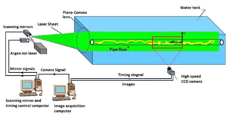
Figure 2.1: Schematic of the LIF system of the Georgia Tech Environmental Fluid Mechanics Laboratory (Tian & Roberts (2003)).

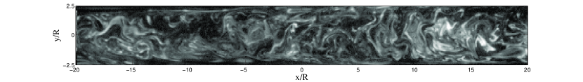
Figure 2.2: LIF experiments: snapshot of the planar fluorescent dye concentration field $C(x,y,t)$ (log scale) tracing turbulent pipe flow patterns at Reynolds number $\mathsf{Re}=3200$ (bulk velocity $U_{b}=6.42\mbox{ cm/s}$, flow from right to left).

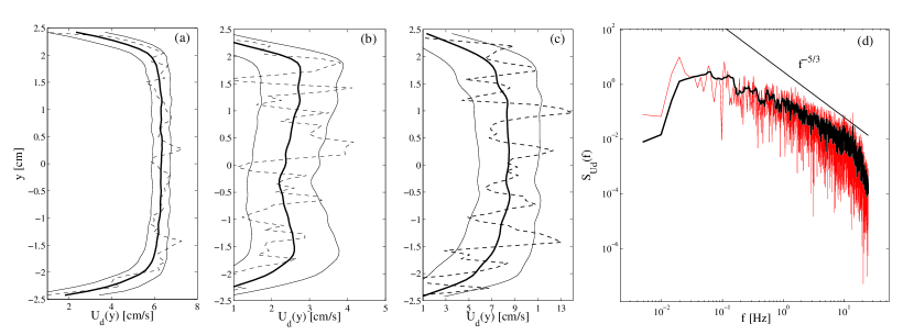
Figure 2.3: Comoving frame velocity profile $U_{d}(y)$ estimated from (a) all space scales, $U_{d,max}$$=6.32$ cm/s, (b) small scales (wavelengths $L_{x}<0.2R$, $L_{y}<0.2R$), $U_{d,max}$$=2.76$ cm/s, and (c) large scales ($L_{x}>2R$, $L_{y}>0.4R$), $U_{d,max}$$=8.52$ cm/s, and pipe radius $R=2.5$ cm; (d) frequency spectrum of the large-scale comoving frame velocity $U_{d}$ [see Eq. (2.4)].

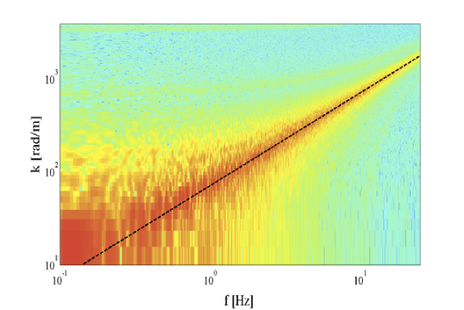
Figure 2.4: Observed frequency-wavenumber spectrum of the fluorescent dye concentration $C(x,y=0,t)$ at the pipe centerline. Estimated mean velocity $U_{m}=\omega/k\sim 8.78$ cm/s (dashed line). $U_{m}/U_{b}=1.37$ and bulk velocity $U_{b}=6.42$ cm/s.

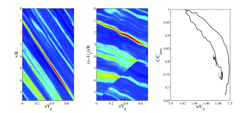
Figure 2.5: LIF experiments: space-time evolution of the dye concentration $C(x,y=0,t)$ at the pipe centerline in the (left) lab frame ($x,t)$ and (center) comoving frame $(x-U_{d}t,t)$; (right) normalized concentration peak intensity $C/C_{max}$ tracked from the initial time $t/T_{d}=0$ ($\Circle$) as function of the observed peak speed $u/U_{d}$, with $C_{max}$ denoting the observed maximum value of $C$. $U_{d}\approx$6.34 m/s and $T_{d}=U_{d}/R$.

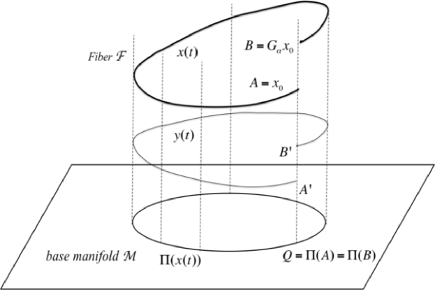
Figure 2.6: Principal fiber bundle: a relative periodic orbit AB reduces to a periodic orbit in the base manifold $\mathcal{M}$ by properly phase-shifting the trajectory along the fiber $\mathcal{F}$ (or Lie-group space). The shift is composed by a dynamical and geometric phases. The shift induced by the dynamical phase yields the comoving trajectory A’C’B’, which is locally transversal to the fibers (parallel transport through the fiber bundle), but it is not a closed trajectory. A further shift by the geometric phase reduces A’C’B’ to a periodic orbit on the base manifold $\mathcal{M}$.

2.2 Data analysis

The vertical comoving frame velocity profile can be estimated from the measured fluorescent dye concentration field $C(x,y,t)$ using Eq. (2.6). For example, Fig. (2.3) shows $U_{d}(y)$ computed accounting for (Panel $a$) all space scales , (Panel $\mathit{b}$) small scales (wavelengths $L_{x}<0.2R$, $L_{y}<0.2R$) and (Panel $c$) large scales of $C$ ($L_{x}>2R$, $L_{y}>0.4R$). Clearly, small scales advect at lower speed than larger scales, in agreement with Krogstad et al. (1998). Moreover, the maximum convective velocity of large scales ($=8.52\mbox{ cm/s}$) is close to the centerline mean flow speed (=$8.78$ cm/s) estimated from the frequency-wavenumber spectrum of $C(x,y=0,t)$ [see Figure (2.4)]. The frequency spectrum of $U_{d}(t)$ estimated from Eq. (2.4) accounting for large scales only is also shown in Panel $d$ of Fig. (2.3). It decays approximately as $f^{-5/3}$ as an indication that the Taylor’s hypothesis is approximately valid, possibly due to the non-dispersive behavior of large scale motions.

In the lab frame $(x,t)$, the space-time evolution of the measured fluorescent dye concentration $C(x,y=0,t)$ at the pipe centerline is shown in the left panel of Figure (2.5). The associated evolution in the comoving frame $\left(x-U_{d}t,t\right)$ is also shown in the center panel. Here, $U_{d}$ is estimated from Eq. (2.4) accounting for all space scales of $C$. Note the pattern-changing dynamics of the passive scalar structures, which still experience a drift in the comoving frame. Moreover, a generic slowdown or decelerated motion is observed as the dye concentration bursts, possibly related to the abovementioned turbulent flow ejections. This is clearly seen in the the right panel of the same Figure, which reports the normalized concentration peak intensity $C/C_{max}$ as function of the observed peak speed $u/U_{d}$, with $C_{max}$ denoting the maximum value of $C$. Further, $u$ is approximately 40-50% larger than the comoving frame velocity $U_{d}$, which is also roughly constant during the event ($U_{d}=6.32\pm 0.22$ cm/s). Note that in oceanic wave groups, large focusing crests tend to slow down as they evolve within the group, as a result of the natural wave dispersion of unsteady wave trains (Banner et al. (2014); Fedele (2014b, a)). Thus, we argue that the observed slowdown of the passive scalar bursts may be due to the wave dispersive nature of small-scale turbulent structures.

In the following, drawing from differential geometry we will study the fiber bundle structure of the state space associated with the fluorescent dye concentration field evolution, which allows to explain the observed excess speed $u-U_{d}$ of concentration bursts in terms of geometric phases of the orbits in the bundle.

3 Principal fiber bundles

The geometric structure of the state space $\mathcal{P}\in\mathbb{R}^{N}$ of a dynamical system with a continuous Lie-group symmetry $G_{\alpha}$ and parameter $\alpha\in\mathbb{\mathcal{\mathbb{R}}}$, is that of a principal fiber bundle: a base manifold $\mathcal{M}$ of dimension $N-1$ (quotient space) and one-dimensional (1-D) fibers attached to any point of $\mathcal{M}$ (e.g. Steenrod (1999); Husemöller (1994)). The fiber $\mathcal{F}$ is the subspace of the Lie group orbit $G_{\alpha}(z)$. One can think of the group as being an action, which pushes points in the bundle around the bundle along the fibers (see Fig. 2.6). For example, the Euclidean space $\mathbb{R}^{3}$ can be seen as a fiber bundle of parallel straight lines. The base manifold is a plane cutting the whole set of parallel lines. This is a trivial fibration since the total space $\mathcal{P}$ is both locally and globally the direct product of the base $\mathcal{M}$ and the fiber $\mathcal{F}$, that is $\mathbb{R}^{3}=\mbox{$\mathcal{M}\text{\texttimes}$$\mathbb{\mathcal{F}=}$}\mathbb{R}^{2}\times\mathbb{R}$. A famous non trivial fiber bundle is the Hopf fibration of $S^{3}$ spheres by great circles $S^{1}$ and base space $S^{2}$ (Hopf (1931), see also Steenrod (1999)). The Hopf fibration, like any fiber bundle, is locally a product space, i.e. $S^{3}=S^{2}\times S^{1}$, but not globally. There are numerous generalizations of it. For example, the unit sphere $S^{2n+1}$ in the complex space $\mathbb{C}^{n+1}$ fibers naturally over the complex projective space $\mathbb{C}P^{n}$ with circles as fibers (see appendix).

A principal fiber bundle is denoted with the quadruplet $(\mathcal{P},\mathcal{M},G_{\alpha},\Pi)$ with total space $\mathcal{P}$ over the base manifold $\mathcal{M}$, and a Lie group $G_{\alpha}$. The map $\Pi:\mathcal{P}\overset{}{\rightarrow}\mathcal{M}$ projects an element $z$ of the state space $\mathcal{P}$ and all the elements of the group orbit $G_{\alpha}(z)$ into the same point $\Pi(z)$ of the base manifold $\mathcal{M}$, viz. $\Pi(z)=\Pi(G_{\alpha}z)$, with $\alpha\in\mathbb{R}$. In $\mathcal{P}$, a trajectory or orbit $z(t)$ can be observed in a special comoving frame, within which the motion is an horizontal transport through the fiber bundle, that is the comoving orbit $y=G_{\alpha_{d}}z$ is locally transversal to the fibers (see Fig. 2.6). The proper shift $\alpha_{d}$ along the fibers to bring the motion in the comoving frame is called dynamical phase. This increases with the time spent by the trajectory to wander around $\mathcal{P}$ and system’s answer to: ” how long did your trip take? ” (Berry (1984)). For example, the translational shift induced by the constant speed of traveling waves, or relative equilibria, is the dynamical phase. They reduce to equilibria within the base manifold $\mathcal{M}$, whereas relative periodic orbits reduce to periodic orbits (see Fig. 2.6). In this case, the shift along the fibers includes also a geometric phase $\alpha_{g}$, induced by the projected motion within the $\mathcal{M}$ (Pancharatnam (1956); Simon (1983); Aharonov & Anandan (1987); Garrison & Chiao (1988)). This phase is independent of time and it depends only upon the curvature of $\mathcal{M}$, and system’s answer to:” where have you been? ” (Berry (1984)).

Geometric phases arise due to anholonomy, that is global change without local change. The classical example is the parallel transport of a vector on a sphere. The change in the vector direction is equal to the solid angle of the closed path spanned by the vector and it can be described by Hannay’s angles (Hannay (1985)). The rotation of Foucault’s pendulum can be explained by means of such a anholonomy. Pancharatnam (1956) discovered this effect for polarized light, and later on Berry (1984) rediscovered it for quantum-mechanical systems. In fluid mechanics, Shapere & Wilczek (1989) exploited geometric phases to explain self-propulsion at low Reynolds numbers. Note that non-periodic orbits in $\mathcal{M}$ induce also a geometric phase, that is the motion does not have to be periodic to have geometric drift (Anandan (1992)).

In summary, the total phase associated with any orbital path on the base manifold is a measure of the motion induced within the fibers of the bundle by the path. In the following, we will propose an Hopf bundle for dynamical systems with translation symmetries.

4 Symmetry reduction via Hopf fibrations

For the sake of simplicity, consider a 1-D space-periodic passive scalar field $C(x,t)$, which evolves according to

$$\partial_{t}C=\mathcal{N}(C),$$ (4.1)

where $\mathcal{N\mathrm{(\mbox{$C$})}}$ is a differential operator of its argument. The extension to higher dimensions is straightforward. The dynamics admits a continuous translation symmetry, that is if $C(x,t)$ is a solution, so is $C(x+x_{s},t)$ for any drift $x_{s}$. It is convenient to express $C$ as the Fourier series

$$\begin{array}[t]{c}C(x,t)=C_{0}(t)+\frac{1}{2}\sum_{m=1}^{N}z_{m}(t)\exp\left(imk_{0}x\right)+c.c.=\\ \\ C_{0}(t)+\sum_{m=1}^{N}\left|z_{m}\right|\cos\left(imk_{0}x+\theta_{m}\right),\end{array}$$ (4.2)

where $C_{0}(t)$ is the mean, $z_{m}=\left|z_{m}\right|\exp(i\theta_{m})$ are complex Fourier amplitudes with phases $\theta_{m}$ and $k_{0}=2\pi/L_{0}$, with $L_{0}$ denoting the domain length. The mean $C_{0}$ is invariant under the group action and it can be decoupled from the vector $z(t)=\{z_{m}\}=\left(z_{1},...z_{N}\right)$. This satisfies the dynamical system

$$\frac{dz}{dt}=\mathcal{\widehat{N}}(z,C_{0}),$$ (4.3)

coupled with

$$\frac{dC_{0}}{dt}=\left\langle\mathcal{N}(C_{0},z)\right\rangle_{x},$$ (4.4)

the space average of (4.1). The vector

$$\mathcal{\widehat{N}}(z,C_{0})=\left\{\widehat{\mathcal{N}}_{m}(z,C_{0})\right\}=\left(\widehat{\mathcal{N}}_{1}(z,C_{0}),...,\widehat{\mathcal{N}}_{N}(z,C_{0})\right),$$ (4.5)

follows from the discrete Fourier transform of $\mathcal{N}$ in Eq. (4.1).

The orbit $z(t)$ wanders in the state space $\mathcal{P}\in\mathbb{C^{\mathrm{\mathit{N}}}}$, and the symmetry group $G_{x_{s}}$ of $z$ is the subspace

$$G_{x_{s}}(z)=\left\{w\in\mathbb{C^{\mathit{N}}}:w=\{z_{m}\exp(imk_{0}x_{s})\},\>\forall x_{s}\in\mathbb{R}\right\}.$$ (4.6)

The state space $\mathcal{P}$ is geometrically a principal fiber bundle: a base manifold $\mathcal{M}$ of dimension $2N-1$ (quotient space) and one dimensional (1-D) fibers $G_{x_{s}}(Z)$ attached to any point $Z\in\mathcal{M}$ (e.g. Steenrod (1999); Husemöller (1994)). The bundle is described by the quadruplet $(\mathcal{P},\mathcal{M},G_{x_{s}},\Pi_{j})$ and the map $\Pi_{j}$ is given as follows. For a non-vanishing Fourier mode $z_{j}$, the desymmetrized orbit $z_{D}(t)$ within the base manifold $\mathcal{M}\in\mathbb{C^{\mathit{N}}}$ is given by the map $\Pi_{j}:\mathit{\mbox{\mbox{$\mathcal{\mathrm{\mathcal{P}}}$}}}\rightarrow\mathcal{M}$

$$z_{D}=\Pi_{j}(z)=Z=(Z_{1},...Z_{m},...Z_{N}),$$ (4.7)

where the complex amplitudes

$$Z_{m}=\left|z_{m}(t)\right|\exp(i\phi_{m}(t)),$$ (4.8)

and phases

$$\phi_{m}=\theta_{m}-\frac{m\theta_{j}}{j}.$$ (4.9)

Note that $Z_{j}$ is real and $\mathcal{M}$ is a $2N-1$ dimensional manifold of $\mathbb{C}^{N}$. For $j>1$, the phase $\theta_{j}$ needs to be unwrapped in order to avoid introducing spurious discrete symmetries. For $j=1$, the fibration reduces to the ’first Fourier mode slice’ proposed in Budanur et al. (2014). The map $\Pi_{j}$ projects an element $z=\{z_{m}\}$ of the state space $\mathcal{P}$ and all the elements of its group orbit $G_{x_{d}}(z)$ into the same point $z_{D}=\Pi_{j}(z)$ in $\mathcal{M}$, namely

$$\Pi_{j}(z)=\Pi_{j}(G_{x_{s}}(z))\mathrm{.}$$ (4.10)

The scalar field $C_{D}$ in the symmetry-reduced frame follows from (4.2) as

$$C_{D}(x,t)=C_{0}(t)+\sum_{m=1}^{N}\left|Z_{m}\right|\cos\left(mk_{0}x+\phi_{m}\right).$$ (4.11)

Note that $\Pi_{j}$ can be written in the equivalent form

$$\begin{array}[t]{c}z_{D}=\Pi_{j}(z)=\left\{z_{m}\left(\frac{\left|z_{j}\right|}{z_{j}}\right)^{m/j}\right\}_{m=1,...N}=\\ \\ \left(z_{1}\left(\frac{\left|z_{j}\right|}{z_{j}}\right)^{1/j},...z_{j-1}\left(\frac{\left|z_{j}\right|}{z_{j}}\right)^{(j-1)/j}\mbox{$,$$\left|z_{j}\right|,z_{j+1}$\text{$\left(\frac{\left|z_{j}\right|}{z_{j}}\right)^{(j+1)/j}$$,...$}$z_{N}\left(\frac{\left|z_{j}\right|}{z_{j}}\right)^{N/j}$}\right),\end{array}$$ (4.12)

which reveals the geometric structure of a Hopf bundle (e.g. Steenrod (1999)). In the following, it is shown that the associated base manifold $\mathcal{M}$, hereafter referred to as $\mathbb{C}T^{n}$, is a generalization of $\mathbb{C}P^{n}$ projective spaces.

4.1 $\mathbb{C}T^{n}$ projective spaces

The complex projective space $\mathbb{C}P^{n}$ is the quotient space of the unit $S^{2n+1}$ hypersphere

$$S^{2n+1}=\left\{z=(z_{1},...z_{n+1})\in\mathbb{C}^{n+1}:\sum_{j=1}^{n+1}\left|z_{j}\right|^{2}=1\right\}$$ (4.13)

with circles $S^{1}$ as fibers under the action of the $U(1)$ group (see also appendix). The projection $\pi_{H}:S^{2n+1}\rightarrow\mathbb{C}P^{n}$ is called the Hopf map. Since $\mathbb{C}P^{1}=S^{2}$ is the Riemann sphere, we obtain the classical Hopf bundle $S^{3}\rightarrow S^{2}$ with fiber $S^{1}$ (Hopf (1931), see also Steenrod (1999)). Hereafter, we generalize $\mathbb{C}P^{n}$ spaces to complex manifolds defined as quotient spaces

$$\mathbb{C}T^{n}=E^{2n+1}/T(1)$$ (4.14)

of the $E^{2n+1}$ hypersurface in $\mathbb{C}^{n+1}$

$$E^{2n+1}=\left\{z=(z_{1},...z_{n+1})\in\mathbb{C}^{n+1}:\sum_{j=1}^{n+1}\left|z_{j}\right|^{\frac{2(n+1)}{j}}=1\right\}$$ (4.15)

under the action of the translation group $T(1)$

$$T_{\lambda}(z)=\left\{Z=(Z_{1},...Z_{n+1})\in\mathbb{C}^{n+1}:Z_{k}=z_{k}\lambda^{k},\quad\left|\lambda\right|=1\right\}.$$ (4.16)

An element $z$ of $\mathbb{C}T^{n}$ is identified with the equivalence class

$$[z]=[z_{1},...z_{n+1}]\sim(\lambda z_{1},...\lambda^{n+1}z_{n+1}),\qquad\lambda\neq 0.$$

Two points of $\mathbb{C}^{n+1}\left\backslash\left\{0\right\}\right.$ are equivalent if they lie on the same subspace or group orbit $T_{\lambda}(z)$. For $n=1$, the group orbit is the space of complex parabolas $z_{2}=\lambda z_{1}^{2}$ ($z_{1}\neq 0$) and, for $n>1$, that of complex hypercurves $z_{n}=\lambda z_{j}^{n/j}$ ($z_{j}\neq 0$). All points of $T_{\lambda}(z)$ reduce to the same point of $\mathbb{C}T^{n}$ and the projection map $\pi:\mathbb{C}^{n+1}\rightarrow\mathbb{C}T^{n}$ can be defined as follows.

The $\mathbb{C}T^{n}$ manifold can be covered by an atlas of charts or slices $U_{j}=\left\{[z]\left|z_{j}\neq 0\right.\right\}\subset\mathbb{C}T^{n}$, where the complex hyperplane $B_{j}=\left\{z_{j}=0\right\}$ is the “border” of $U_{j}$ (Siminos & Cvitanović (2011)). Then, the projection onto a chart or slice $U_{j}$ is given by the map $\pi_{j}:\mathbb{C}^{n+1}\rightarrow U_{j}$

$$\pi_{j}([z])=\pi_{j}([z_{1},...z_{n+1}])=\left\{z_{k}\left(\frac{\left|z_{j}\right|}{z_{j}}\right)^{k/j}\right\}_{k=1,...n+1},$$ (4.17)

which is the same map as in Eq. (4.12) for $n=N-1$. Thus, the fiber bundle formulated in the previous section is generalization of a Hopf fibration for dynamical systems with $T(1)$ symmetries. The associated state space fibrates over a $\mathbb{C}T^{n}$ manifold with fibers as the hypercurves $T_{\lambda}(z)$. fibrates over a $\mathbb{C}T^{n}$ manifold with fibers as the hypercurves $T_{\lambda}(z)$. Within the charts or slices, relative equilibria reduce to equilibria and relative periodic orbits reduce to periodic orbits. Clearly, when $z_{j}$ approaches zero, but likely never completely vanishes, the trajectory in $\mathbb{C}T^{n}$ wanders nearby the border $B_{j}$ of the slice $U_{j}$ and the associated geometric phase tends to become singular (see, for example, Budanur et al. (2014)). As described in Siminos & Cvitanović (2011), a different chart can then be chosen and the charts’ borders can be glued together via ridges into an atlas that spans the state space region of interest.

4.2 Dynamical and geometric phases

The desymmetrized orbit $z_{D}(t)=Z(t)=\left\{Z_{m}(t)\right\}$ within the base manifold $\mathcal{M}$ is determined by properly shifting $z(t)=\left\{z_{m}(t)\right\}$ along the fibers by $x_{s}(t)$, that is $Z=G_{-x_{s}}(z)$ and components

$$z_{m}=Z_{m}\exp(imk_{0}x_{s}),\qquad m=1,...N,$$ (4.18)

To find $x_{s}$, we impose the condition of transversality to the fiber or group orbit

$$\overline{T_{x_{s}}(Z)}\frac{dZ}{dt}=0,$$ (4.19)

namely the tangent $\frac{dZ}{dt}$ at $Z$ must be orthogonal to the group tangent space

$$T_{x_{s}}(Z)=(G_{x_{s}}^{-1}\partial_{x_{s}}G)Z=\{imk_{0}Z_{m}\}.$$ (4.20)

From (4.3) and (4.18), (4.19) yields

$$\overline{T_{x_{s}}(Z)}\left(\frac{dZ}{dt}+\frac{dx_{s}}{dt}T_{x_{s}}(Z)-\widehat{\mathcal{N}}(Z,C_{0})\right)=0,$$

from which

$$\frac{dx_{s}}{dt}=\frac{dx_{d}}{dt}+\frac{dx_{g}}{dt},$$ (4.21)

where

$$\frac{dx_{d}}{dt}=U_{d}=\frac{\mathrm{Re}\left[\overline{T_{x_{s}}(Z)}\widehat{\mathcal{N}}(Z,C_{0})\right]}{\left|T_{x_{s}}(Z)\right|^{2}}=-\frac{\mathrm{Im}\sum mk_{0}\overline{Z_{m}}\widehat{\mathcal{N}}_{m}(Z,C_{0})}{\sum m^{2}k_{0}^{2}\left|Z_{m}\right|^{2}}$$ (4.22)

is the velocity associated with the dynamical phase $x_{d}$, and

$$\frac{dx_{g}}{dt}=U_{g}=-\frac{\mathrm{Re}\left(\overline{T_{x_{s}}(Z)}\frac{dZ}{dt}\right)}{\left|T_{x_{s}}(Z)\right|^{2}}=\frac{\mathrm{Im}\sum mk_{0}\overline{Z_{m}}\frac{dZ_{m}}{dt}}{\sum m^{2}k_{0}^{2}\left|Z_{m}\right|^{2}}$$ (4.23)

is that associated with the geometric phase $x_{g}$. Here, the sum is over $m=1,...N$ and $\mathrm{\mathrm{Re}\mbox{$(\mbox{$a$})$},Im}(a)$ denote the real and imaginary parts of $a$. Note that $\overline{T_{x_{s}}(Z)}\widehat{\mathcal{N}}(Z,C_{0})$ and $\left|T_{x_{s}}(Z)\right|^{2}$ in (4.22) are invariant under the $T(1)$ group action, and $x_{d}$ can also be determined replacing $Z$ with the orbit $z$ in $\mathcal{P}$, which is usually known or observable in applications. The total shift or drift

$$x_{s}=x_{d}+x_{g},$$ (4.24)

where

$$x_{d}(t)=\int_{0}^{t}V_{d}d\tau,\qquad x_{g}(t)=\int_{0}^{t}V_{g}d\tau.$$ (4.25)

For the Hopf bundle given by the map (4.7) or equivalently (4.12), the total drift

$$x_{s}=-\frac{\theta_{j}}{k_{0}j},\qquad j\geq 1.$$

The dynamical phase $x_{d}$ increases with the time spent by the trajectory $z(t)$ to wander around $\mathcal{P}$, whereas the geometric phase $x_{g}$ depends upon the path $\gamma$ associated with the motion of $Z(t)$ in the base manifold $\mathcal{M}$. Indeed, from (4.23) $x_{g}$ can be rewritten as the path integral

$$x_{g}=-\int_{\gamma}\frac{\mathrm{Re}\left(\overline{T_{x_{s}}(Z)}dZ\right)}{\left|T_{x_{s}}(Z)\right|^{2}}=\int_{\gamma}\frac{\mathrm{Im}\sum mk_{0}\overline{Z_{m}}dZ_{m}}{\sum m^{2}k_{0}^{2}\left|Z_{m}\right|^{2}}.$$ (4.26)

Clearly, the geometric phase is independent of time and it depends only upon the reduced motion within $\mathcal{M}$.

It is straightforward to recognize that $U_{d}$ in (4.22) is the comoving frame velocity introduced in (2.4) and specialized for the dynamical system (4.3). In particular, if we shift the orbit $z(t)$ along the fibers by $x_{d}(t)$, we obtain the comoving frame orbit

$$Z_{d}(t)=G_{-x_{d}}(z)=\left\{z_{m}(t)\exp(-imk_{0}x_{d}(t)\right\}$$

that moves through the fiber bundle locally transversal to the fibers. This motion is referred to as an “horizontal transport” through the fiber bundle. In physical space, this corresponds to an evolution in the comoving frame $\left(x-U_{d}t,t\right)$ (see Fig. (2.5)). In general, $Z_{d}$ still experiences a shift, the geometric $x_{g}$, if any. Indeed, the projected path $z_{D}=Z$ within the base manifold $\mathcal{M}$ is obtained by further shifting $Z_{d}$ along the fibers by $x_{g}$ (see Fig. 2.6), namely

$$Z(t)=G_{-x_{g}}(Z_{d})=G_{-x_{d}-x_{g}}(z)=\left\{z_{m}(t)\exp\left[-imk_{0}\left(x_{d}+x_{g}\right)\right]\right\}.$$

In physical space, this corresponds to a pattern-changing dynamics in the symmetry-reduced frame $\left(x-(U_{d}+U_{g})t,t\right)$ as discussed later on. Only relative equilibria or traveling waves have null geometric phase, since their pattern is not dynamically changing in the base manifold as they reduce to equilibria. In this case the comoving and symmetry-reduced frames are the same.

5 Symmetry reduction of LIF data

In this section, we apply Hopf fibrations to symmetry-reduce LIF measurements of turbulent pipe flows at $\mathsf{Re}=3200$ (see section 2.1). Figure (5.1) illustrates the space-time evolution of a passive scalar burst event. The left panel shows the fluorescent dye concentration $C(x,y=0,t)$ at the pipe centerline in the lab frame $(x,t)$. A drift in the streamwise direction $x$ is observed. The corresponding orbit $z(t)$ in the subspace {$\mbox{Re}(z_{11}),\mbox{Im}(z_{13}),\mbox{Re}(z_{15})$} of the state space $\mathcal{P}$ of dimensions $N=65\times 622=40430$ is shown in the left panels of Fig. (5.2). Note that the excursion of the orbit while the concentration $c$ lingers above the threshold $0.8C_{max}$ is complicated (bold line) since it wanders around its group orbit $G_{x_{s}}(z)$ as a result of the drift induced by the translation symmetry. The center panel of Fig. (5.1) shows the space-time evolution in the comoving frame $\left(x-U_{d}t,t\right)$. Note that the dye concentration patterns still experience a significant drift, the geometric phase $x_{g}$ at velocity $U_{g}$ [see Eqs. (4.23),(4.26)]. As a result, the associated orbit in state space still wanders around the group orbit $G_{x_{s}}(z)$. The drift disappears in the symmetry-reduced frame $\left(x-(U_{d}+U_{g})t,t\right)$ associated with the dynamics in the chart or slice $U_{36}$ of the base manifold $\mathcal{M}$, as shown in the right panel of Figure (5.1). Here, one slice is sufficient to symmetry-reduce the orbit $z$ over the analyzed time span as its component $z_{36}$ never lingers closely near zero. A pattern-changing dynamics of the passive scalar structures is revealed as clearly seen in Figure (5.3). The corresponding symmetry-reduced orbit $z_{D}(t)=Z(t)$, computed from Eq. (4.7), is shown in the right panels of Fig. (5.2) and plotted in the subspace {$\mbox{Re}(Z_{11}),\mbox{Im}(Z_{13}),\mbox{Re}(Z_{15})$} of $\mathcal{M}$. Here, the excursion of the orbit while the concentration $C$ is high (bold line) indicates an homoclinic type behavior.

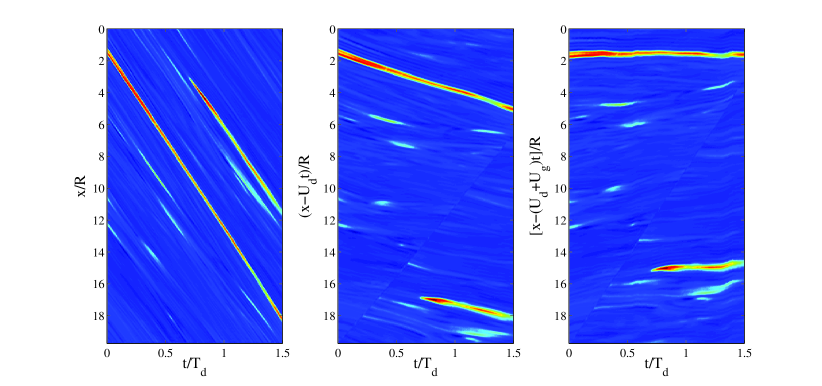
Figure 5.1: Symmetry reduction of LIF data: space-time evolution of a passive scalar burst event; measured concentration $C(x,y=0,t)$ at the pipe centerline in the (left) lab frame $(x,t)$, (center) comoving frame $\left(x-U_{d}t,t\right)$ and (right) symmetry-reduced frame $\left(x-(U_{d}+U_{g})t,t\right)$; time average $U_{d}\approx 6.74$ cm/s, $U_{g}\approx 0.4U_{d}$ and $T_{d}=U_{d}/R$.

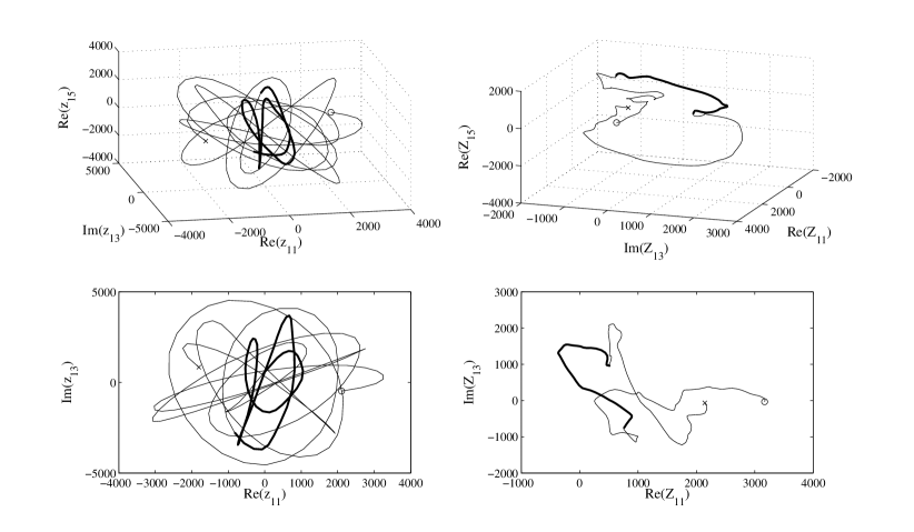
Figure 5.2: Symmetry reduction of LIF data: (left) Orbit trajectories in the subspace ($\mbox{Re}(z_{11}),\mbox{Im}(z_{13}),\mbox{Re}(z_{15})$) of the state space $\mathcal{P}$ associated with the passive scalar dynamics in the lab frame of Fig. 7; (right) corresponding symmetry-reduced orbit within the chart or slice $U_{36}$ of the base manifold $\mathcal{M}$ (subspace ($\mbox{Re}(Z_{11}),\mbox{Im}(Z_{13}),\mbox{Re}(Z_{25})$). The bold line indicates the excursion of the orbit while the concentration $C$ lingers above the threshold $0.8C_{max}$ ($\Circle$ =initial time, $\times$=final time).

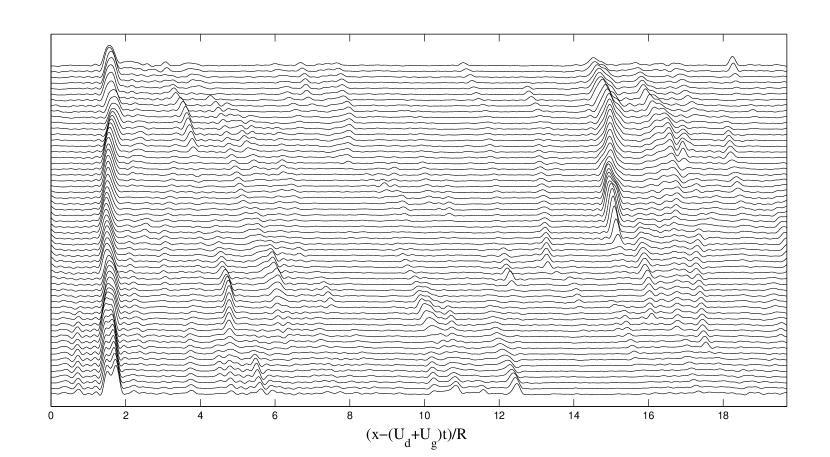
Figure 5.3: Symmetry reduction of LIF data: pattern-changing profiles at increasing instants of time (from bottom to top) of the measured concentration $C(x,y=0,t)$ at the pipe centerline in the symmetry-reduced frame $\left(x-(U_{d}+U_{g})t,t\right)$. Associated 2-D pattern is shown in the right panel of Fig. (5.1).

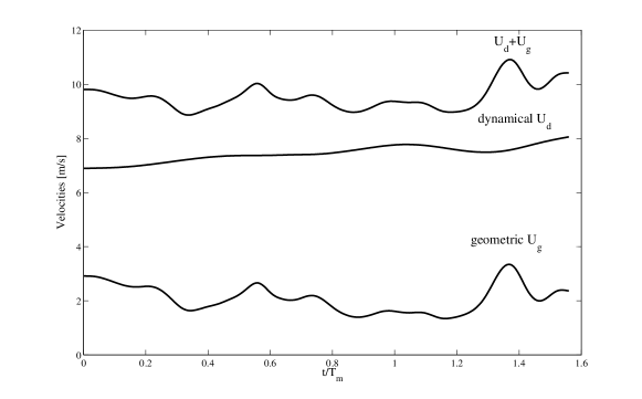
Figure 5.4: Symmetry reduction of LIF data: dynamical and geometric velocities $U_{d}$ and $U_{g}$ associated with the orbit in state space of Fig. (5.2).

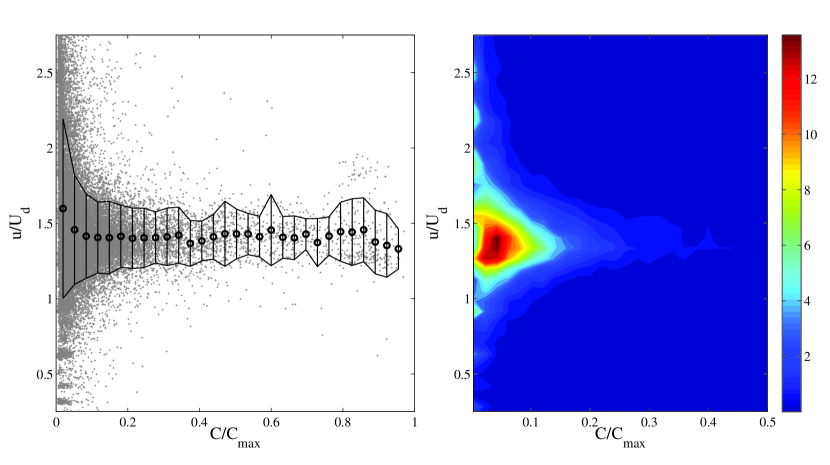
Figure 5.5: LIF experiments: (left) observed normalized dye concentration peak speed $u/U_{d}$ as function of the amplitude peak $C/C_{max}$, and (right) associated probability density function.

Note that the speed $u\approx U_{d}+U_{g}$ of the dye concentration burst is approximately 40% larger than the comoving frame velocity $U_{d}$, which slighlty changes during the event, whereas the geometric phase velocity $U_{g}\approx 0.4U_{d}$ as seen in Figure (5.4). This appears a generic trend of the flow as clearly seen in Fig. 5.5, which shows the observed normalized speed $u/U_{d}$ of dye concentration peaks tracked in space as function of their amplitude $C/C_{max}$, and the associated probability density function. As the peak amplitude of concentration bursts increases, their speed $u$ tend to be close to $1.43U_{d}$. Thus, the space-time evolution in the comoving frame cannot explain the excess speed $\delta u=u-U_{d}$ (see center panel of Fig. 5.4). Indeed, $\delta u$ is roughly the geometric phase velocity $U_{g}$ induced by the motion in the symmetry-reduced state space $\mathcal{M}$. In physical space, this results in the pattern-changing dynamics of the passive scalar structures revealed in the symmetry-reduced frame (see Figure (5.3)). Only when geometric phases are small, viz. $U_{g}\ll U_{d}$, Taylor’s approximation is valid and the flow structures slightly deform as they are advected at the comoving frame speed $U_{d}$.

6 Conclusions

We have presented a theoretical study on the fiber bundle structure of the state space of dynamical systems with continuous translation symmetries. A generalization of Hopf fibrations is proposed to quotient such symmetries in the complex manifold $\mathbb{C}T^{n}$, which generalizes $\mathbb{C}P^{n}$ projective spaces. As an application, we have exploited LIF techniques to capture planar fluorescent dye concentration fields tracing a turbulent pipe flow at Reynolds number $\mathsf{Re}=3200$. The symmetry reduction of LIF measurements unveils that the motion of the passive scalar structures is associated with the dynamical and geometric phases of the corresponding orbits in the Hopf bundle. In particular, the observed speed $u\approx U_{g}+U_{d}\approx 1.43U_{d}$ of dye concentration bursts exceeds the comoving or convective velocity $U_{d}$. The excess speed $u-U_{d}$ can be explained in terms of the pattern-changing dynamics in the symmetry-reduced frame and associated geometric phase velocity $U_{g}\approx 0.43U_{d}.$

Hopf fibrations are promising for symmetry reduction of three-dimensional LIF and PIV measurements as well as simulated flows of pipe turbulence, in order to unveil the skeleton of its chaotic dynamics in state space. Further studies along these directions are desirable.

7 Acknowledgments

FF acknowledges the Georgia Tech graduate courses “Classical Mechanics II” taught by Prof. Jean Bellissard in Spring 2013 and “Nonlinear dynamics: Chaos, and what to do about it¿‘ taught by Prof. Predrag Cvitanovic in Spring 2012. FF also thanks Prof. Alfred Shapere for discussions on geometric phases, and Profs. Predrag Cvitanovic, Bruno Eckhardt and Dr. Evangelos Siminos for discussions on symmetry reduction.

8 Appendix: $\mathbb{C}P^{n}$ complex projective spaces

A $\mathbb{C}P^{n}$ space is the set of 1-dimensional complex-linear subspaces, or lines of the complex space $\mathbb{C}^{n+1}$. In particular, $\mathbb{C}P^{n}$ is the quotient of $\mathbb{C}^{n+1}\left\backslash\left\{0\right\}\right.$ by the equivalent relation

$$z\sim w\Longleftrightarrow\exists\lambda\in\mathbb{C}\left\backslash\left\{0\right\}\right.:\>w=\lambda z,\qquad\left|\lambda\right|=1.$$ (8.1)

Two points of $\mathbb{C}^{n+1}\left\backslash\left\{0\right\}\right.$are equivalent iff they lie on the same line, viz. they are complex linear independent. We denote the equivalence class of $z$ by $[z]$, which is an element of the $U(1)$ group.

The projection map $\pi:\mathbb{C}^{n+1}\rightarrow\mathbb{C}P^{n}$ can be defined as follows. Consider

$$z=(z_{1},...z_{n+1})\in\mathbb{C}^{n+1},\qquad z\neq 0,$$ (8.2)

then $\mathbb{C}P^{n}$ is a complex manifold, which can be covered by charts $U_{j}=\left\{[z]\left|z_{j}\neq 0\right.\right\}\subset\mathbb{C}P^{n}$, i.e. the space of all lines not contained in the complex hyperplane or border $B_{j}=\left\{z_{j}=0\right\}$. Then, the maps $\pi_{j}:\mathbb{C}^{n+1}\rightarrow U_{j}$ are defined as

$$\begin{array}[t]{c}\pi_{j}([z])=\pi_{j}([z_{1},...,z_{n+1}])=\left(z_{k}\left(\frac{\left|z_{j}\right|}{z_{j}}\right)\right)_{k=1,...n+1}\\ \\ \left(z_{1}\left(\frac{\left|z_{j}\right|}{z_{j}}\right),...z_{j-1}\left(\frac{\left|z_{j}\right|}{z_{j}}\right),\left|z_{j}\right|,z_{j+1}\left(\frac{\left|z_{j}\right|}{z_{j}}\right),...z_{n+1}\left(\frac{\left|z_{j}\right|}{z_{j}}\right)\right).\end{array}$$ (8.3)

It is straightforward to see that $\mathbb{C}P^{n}$ is the quotient space of a unit $S^{2n+1}$ sphere under the action of the $U(1)$ group, namely

$$\mathbb{C}P^{n}=S^{2n+1}/U(1).$$ (8.4)

Indeed, every line in $\mathbb{C}^{n+1}$ intersects the unit $S^{2n+1}$ sphere in a circle $S^{1}$, and we obtain a point of $\mathbb{C}P^{n}$ defined by this line by identifying all points on $S^{1}$.

References

- Aharonov & Anandan (1987) Aharonov, Y. & Anandan, J. 1987 Phase change during a cyclic quantum evolution. Phys. Rev. Lett. 58, 1593–1596.
- Anandan (1992) Anandan, Jeeva 1992 The geometric phase. Nature 360 (6402), 307–313.
- Banner et al. (2014) Banner, M. L., Barthelemy, X., Fedele, F., Allis, M., Benetazzo, A., Dias, F. & Peirson, W. L. 2014 Linking reduced breaking crest speeds to unsteady nonlinear water wave group behavior. Phys. Rev. Lett. 112, 114502.
- Berry (1984) Berry, M. V. 1984 Quantal phase factors accompanying adiabatic changes. Proceedings of the Royal Society of London. A. Mathematical and Physical Sciences 392 (1802), 45–57.
- Budanur et al. (2014) Budanur, N. B., Cvitanović, P., Davidchack, R. L. & Siminos, E. 2014 Reduction of so(2) symmetry for spatially extended dynamical systems.
- Chandler & Kerswell (2013) Chandler, G. J. & Kerswell, R. R. 2013 Invariant recurrent solutions embedded in a turbulent two-dimensional kolmogorov flow. Journal of Fluid Mechanics 722, 554–595.
- Cvitanović (2013) Cvitanović, Predrag 2013 Recurrent flows: the clockwork behind turbulence. Journal of Fluid Mechanics 726, 1–4.
- Cvitanović et al. (2013) Cvitanović, P., Artuso, R., Mainieri, R., Tanner, G. & Vattay, G. 2013 Chaos: Classical and quantum.
- Cvitanovic & Eckhardt (1991) Cvitanovic, P. & Eckhardt, B. 1991 Periodic orbit expansions for classical smooth flows. Journal of Physics A: Mathematical and General 24 (5), L237.
- Del Álamo & Jimenez (2009) Del Álamo, J. C. & Jimenez, J. 2009 Estimation of turbulent convection velocities and corrections to taylor’s approximation. Journal of Fluid Mechanics 640, 5–26.
- Faisst & Eckhardt (2003) Faisst, H. & Eckhardt, B. 2003 Traveling waves in pipe flow. Phys. Rev. Lett. 91 (22), 224502.
- Fedele (2014a) Fedele, F. 2014a Geometric phases of water waves.
- Fedele (2014b) Fedele, Francesco 2014b On certain properties of the compact zakharov equation. Journal of Fluid Mechanics 748, 692–711.
- Froehlich & Cvitanović (2012) Froehlich, S. & Cvitanović, P. 2012 Reduction of continuous symmetries of chaotic flows by the method of slices. Communications in Nonlinear Science and Numerical Simulation 17 (5), 2074 – 2084.
- Garrison & Chiao (1988) Garrison, J. C. & Chiao, R. Y. 1988 Geometrical phases from global gauge invariance of nonlinear classical field theories. Phys. Rev. Lett. 60, 165–168.
- Gibson et al. (2008) Gibson, J. F., Halcrow, J. & Cvitanović, P. 2008 Visualizing the geometry of state space in plane couette flow. Journal of Fluid Mechanics 611, 107–130.
- Gritsun (2011) Gritsun, A. 2011 Connection of periodic orbits and variability patterns of circulation for the barotropic model of atmospheric dynamics. Doklady Earth Sciences 438 (1), 636–640.
- Gritsun (2013) Gritsun, A. 2013 Statistical characteristics, circulation regimes and unstable periodic orbits of a barotropic atmospheric model. Philosophical Transactions of the Royal Society A: Mathematical, Physical and Engineering Sciences 371 (1991).
- Hannay (1985) Hannay, J H 1985 Angle variable holonomy in adiabatic excursion of an integrable hamiltonian. Journal of Physics A: Mathematical and General 18 (2), 221.
- Hopf (1931) Hopf, Heinz 1931 Über die abbildungen der dreidimensionalen sphäre auf die kugelfläche. Mathematische Annalen 104 (1), 637–665.
- Husemöller (1994) Husemöller, Dale 1994 Fibre Bundles, 3rd edn. Graduate Texts in Mathematics, Book 20 1. New York, Springer.
- Kreilos et al. (2014) Kreilos, T., Zammert, S. & Eckhardt, B. 2014 Comoving frames and symmetry-related motions in parallel shear flows. Journal of Fluid Mechanics 751, 685–697.
- Krogstad et al. (1998) Krogstad, P.-Å., Kaspersen, J. H. & Rimestad, S. 1998 Convection velocities in a turbulent boundary layer. Physics of Fluids 10 (4), 949–957.
- Pancharatnam (1956) Pancharatnam, S. 1956 Generalized theory of interference, and its applications. Proceedings of the Indian Academy of Sciences - Section A 44 (5), 247–262.
- Rowley et al. (2003) Rowley, C. W., Kevrekidis, I. G., Marsden, J. E. & K., Lust 2003 Reduction and reconstruction for self-similar dynamical systems. Nonlinearity 16 (4), 1257.
- Rowley & Marsden (2000) Rowley, Clarence W. & Marsden, Jerrold E. 2000 Reconstruction equations and the karhunen–loève expansion for systems with symmetry. Physica D: Nonlinear Phenomena 142 (1–2), 1 – 19.
- Shapere & Wilczek (1989) Shapere, Alfred & Wilczek, Frank 1989 Geometry of self-propulsion at low reynolds number. Journal of Fluid Mechanics 198, 557–585.
- Siminos & Cvitanović (2011) Siminos, E. & Cvitanović, P. 2011 Continuous symmetry reduction and return maps for high-dimensional flows. Physica D: Nonlinear Phenomena 240 (2), 187 – 198.
- Simon (1983) Simon, Barry 1983 Holonomy, the quantum adiabatic theorem, and berry’s phase. Phys. Rev. Lett. 51 (24), 2167–2170.
- Steenrod (1999) Steenrod, Norman 1999 The Topology of Fibre Bundles. Princeton, University Press.
- Taylor (1938) Taylor, G. I. 1938 The spectrum of turbulence. Proceedings of the Royal Society of London. Series A - Mathematical and Physical Sciences 164 (919), 476–490.
- Tian & Roberts (2003) Tian, X. & Roberts, P. J.W. 2003 A 3d lif system for turbulent buoyant jet flows. Experiments in Fluids 35 (6), 636–647.
- Viswanath (2007) Viswanath, D. 2007 Recurrent motions within plane couette turbulence. Journal of Fluid Mechanics 580, 339–358.
- Wedin & Kerswell (2004) Wedin, H. & Kerswell, R. R. 2004 Exact coherent structures in pipe flow: travelling wave solutions. Journal of Fluid Mechanics 508, 333–371.
- Willis et al. (2013) Willis, A. P., Cvitanović, P. & Avila, M. 2013 Revealing the state space of turbulent pipe flow by symmetry reduction. Journal of Fluid Mechanics 721, 514–540.