Statistical Mechanics of Hamiltonian Adaptive Resolution Simulations

Abstract

The Adaptive Resolution Scheme (AdResS ) is a hybrid scheme that allows to treat a molecular system with different levels of resolution depending on the location of the molecules. The construction of a Hamiltonian based on the this idea (H-AdResS ) allows one to formulate the usual tools of ensembles and statistical mechanics. We present a number of exact and approximate results that provide a statistical mechanics foundation for this simulation method. We also present simulation results that illustrate the theory.

I Introduction

Biological and soft matter systems are characterized by the existence of processes with many different length and time scales. These processes are usually coupled, making their theoretical, experimental, and computer simulation description a daunting task. The functioning of a protein, for example, involves chemical processes at active sites as well as the overall dynamics of the protein and its environment Neri et al. (2005). Crack propagation is another example in which the atomic processes occuring at the crack tip affect crucially the overall elastic behaviour of the sample, and vice-versa Csányi et al. (2004). From a computational point of view, the brute force approach of treating the system with full molecular detail is not possible, and one needs to deal with simplified, or coarse-grained versions of the system Voth (2009). By definition, in any coarse-grained model some atomic/molecular detail is lost. In some fortunate cases, the need for atomistic detail is confined in small regions of space as in the examples above, and there is hope that a hybrid scheme coupling all atom (AA) with coarse-grained (CG) descriptions may be a successful approach. The coupling of different models describing the system at different resolutions is an active field of research Park and Heyden (2009); Wang et al. (2013) and in our opinion it will become useful in a broad range of calculations, beyond the multi-scale community Wang et al. (2013).

We have recently developed an Hamiltonian Adaptive Resolution Scheme (H-AdResS ) Potestio et al. (2013a, b). Other proposals for Hamiltonian hybrid (AA/CG) schemes have been presented Park and Heyden (2009) which are technically challenging as compared with H-AdResS . As opposed to previous versions of AdResS, where a force interpolation principle was the crucial element, in H-AdResS potentials are interpolated. The proposed Hamiltonian in H-AdResS includes a switching field that allows for a swift interpolation between the truly microscopic Hamiltonian and a CG version of it. When a molecule crosses the interface between the AA and CG regions, its interaction with other molecules changes accordingly. Usually the CG potential of interaction used in the CG region is only an approximate version of the actual potential of mean force. The discrepancies between the CG potential and the potential of mean force are taken into account in the H-AdResS Hamiltonian through a free energy compensation term Potestio et al. (2013a, b).

The idea of interpolating AA an CG potentials through a hybrid region is not new and was introduced in Refs. Ensing et al. (2007),Nielsen et al. (2010) under the name of adaptive Multiscale Molecular Dynamics (MMD)Nielsen et al. (2010). However, the detailed form of the interpolation is slightly different in H-AdResS and leads to the existence of a well-defined Hamiltonian that allows for the natural use of the principles of Statistical Mechanics. In the original version of MMD, energy was not conserved Delle Site (2007),Praprotnik et al. (2011) and thermostats were required Ensing et al. (2007),Nielsen et al. (2011). In the original thermostatted AdResS Praprotnik et al. (2007) and also in more recent versions Wang et al. (2013), the mass in the atomistic domain fluctuates according to the Grand-Canonical ensemble; at least up to the second moment of the probability density function, as it has numerically Delgado-Buscalioni et al. (2008a), and theoretically shown Wang et al. (2013). Density fluctuations are determined by the fluid compressibility, specified by the integral of the radial distribution function, and by finely tunning the CG potential one can match the compressilibities of the CG and AA domains. Having the same compressibility does not however ensure the same pressure equation of state and to ensure a constant density profile over the CG and AA domains, a recent work Fritsch et al. (2012) proposes the imposition of a “correction force field”, which is iteratively evaluated according to the idea of imposing pressure balance (and thus involving compressibilities). The existence of a Hamiltonian permits us to derive a fundamental relation between the force density and the density gradient, which turns out to be independent on the compressibility. This relation explains the basis of the “correction force field” used to control the density profile, not only in Ref. Fritsch et al. (2012) but also in many other algorithms using domain decomposition (see e.g. Refs. Issa and Poesio (2014); Kotsalis et al. (2007)).

The Hamiltonian system of H-AdResS also allows to extend the working ensemble also to the $E,N,V$ microcanonical ensemble, with no need of any extraneous thermostats. However, the benefits of a Hamiltonian description will prove to be substantially broader, as already shown in Ref. Potestio et al. (2013b).

In the present paper, we derive the Statistical Mechanics basis for the H-AdResS method. Several exact results concerning the local equations of state for the pressure and temperature allow for the formulation of the free energy compensation term in an iterative way. We also show that under a local equilibrium approximation, valid when the hybrid region is wide, the iterative procedure can be simplified leading to an approximate but very efficient way for the calculation of the free energy compensation term in the Hamiltonian. We have analyzed the effect of the width of the transition layer where molecules gradually change their resolution. A relevant outcome is that the H-AdResS total free energy compensation is independent on the layer, even for widths of the same order of the molecular diameter. Another very important observation is that the H-AdResS total free energy correction is equal, within error bars, to the free energy difference between both fluids (atomistic and coarse-grained) evaluated from Kirkwood thermodynamic integration Kirkwood (1935). Although more research is required in this direction, this would allow H-AdResS to be used as a flexible tool for estimation of free energy differences in different scenarios.

In what follows, we first present the H-AdResS Hamiltonian formulation in Sec. II. The free energy corresponding to the H-AdResS Hamiltonian is introduced in Sec. III. In Sec. IV we derive expressions for the temperature and the pressure tensor fields. In Sec. V we demonstrate that the condition of constant pressure over the H-AdResS simulation stems from the condition of translational invariance of the free energy. The force balance equation derived in Sec. VI permits to rationalize the different types of H-AdResS compensation terms, for either constant pressure or density fields. Section VII shows that under local equilibrium (LE) conditions, the FEC is just the Kirkwood free energy difference Kirkwood (1935), thus justifying the non-iterative route used in our previous works Potestio et al. (2013a, b). Finally, the theoretical framework is validated through simulations in Sec. VIII where we also provide relaxational schemes for the iterative route to the FEC. We also study the effect of the transition layer width and the deviation from the Kirkwood approximation to the FEC. Conclusions and some future perspectives are given in Sec. IX.

II The AdResS Hamiltonian

Consider a classic molecular system composed of $N$ constituent atoms. The microscopic state of the system is described by the positions and momenta of the atoms, denoted generically by $r,p$. The system is coarse-grained by considering the centers of mass (CoM) of $M$ groups of atoms that are bound together and that are termed blobs. A blob may be, for example, a single molecule or a part of a bigger molecule. The position of the $\mu$-th blob CoM is $\hat{\bf R}_{\mu}$ which is defined as the following phase function

$$\hat{\bf R}_{\mu}(r) =\sum_{i}^{N}\delta_{\mu}(i){\bf r}_{i}\frac{m_{i}}{M_{\mu}}=\sum^{N_{\mu}}_{i_{\mu}}{\bf r}_{i_{\mu}}\frac{m_{i_{\mu}}}{M_{\mu}}$$

$$M_{\mu} =\sum_{i}^{N}\delta_{\mu}(i)m_{i}$$ (1)

where the indicator symbol $\delta_{\mu}(i)$ takes the value 1 if atom $i$ is in blob $\mu$ and zero otherwise. The last definition makes use of the notation $i_{\mu}$ that corresponds to the $i$-th atom of blob $\mu$ and ${N_{\mu}}$ is the number of atoms of blob $\mu$. The microscopic Hamiltonian governing the dynamics of the atoms is

$$H^{1}(r,p) =\sum_{i}^{N}\frac{{\bf p}_{i}^{2}}{2m_{i}}+\sum_{\mu}^{M}V^{\rm intra}_{\mu}(r)+V^{1}(r)$$ (2)

where the total potential energy of interaction of the atoms is decomposed into the potential of interaction between atoms within a blob $V^{\rm intra}_{\mu}(r)$ and the potential of interaction between atoms of different blobs $V^{1}$. This potential energy can be decomposed as $V^{1}=\sum_{\mu}^{M}V^{1}_{\mu}$ where the terms $V^{1}_{\mu}(r)$ are the potential energy of interaction of the atoms of different blobs where one of the atoms of the pair is in blob $\mu$. Explicitly

$$V^{1}_{\mu}(r) =\frac{1}{2}\sum_{ij}^{N}\delta_{\mu}(i)\phi^{\rm inter}(r_{ij})$$ (3)

where $\phi^{\rm inter}$ is the pair potential between atoms $i,j$ of different blobs. It is understood that $\phi^{\rm inter}(r_{ij})$ is zero if atoms $i,j$ belong to the same blob. Note that any Hamiltonian that differs from the one in Eq. (2) by a constant term will produce exactly the same dynamics. The usual convention is to chose the zero of potential energy in such a way that when the particles are very far apart and, therefore, non-interacting, the potential energy is zero. This fixes the origin of the energy scale. We will assume that the above Hamiltonian has, through a mixing property of its Hamiltonian flow, a well defined equilibrium ensemble. For this to be true it is necessary that the finite system of $N$ atoms were confined, either by a time-independent external field (not included in (2)) or through periodic boundary conditions.

The central idea of H-AdResS is to introduce a switching field $\lambda({\bf r})$ that takes the value 1 in the region of space where the system is described in full all atomic (AA) detail, and the value 0 in the region of space where the system is described in a coarse-grained (CG) way. In the transition region between the two zones the switching field changes monotonously from 0 to 1. The field $\lambda({\bf r})$ gives the degree of detail of the description. Instead of the microscopic Hamiltonian (2), the dynamics of the atoms is modified with the following H-AdResS Hamiltonian,

$$H_{[\lambda]}(r,p) =\sum_{i}^{N}\frac{{\bf p}_{i}^{2}}{2m_{i}}+V_{[\lambda]}(r)$$

$$V_{[\lambda]}(r) =\sum_{\mu}^{M}V^{\rm intra}_{\mu}(r)+\sum_{\mu}^{M}\lambda(\hat{\bf R}_{\mu})V^{1}_{\mu}(r)$$

$$+\sum_{\mu}^{M}(1-\lambda(\hat{\bf R}_{\mu}))V^{0}_{\mu}(R)+\sum_{\mu}^{M}{\cal F}(\lambda(\hat{\bf R}_{\mu}))$$ (4)

The potential $V^{0}_{\mu}(R)$ is assumed to depend on the atomic coordinates $r$ only through the position of the centers of mass, denoted collectively as $R=\{\hat{\bf R}_{\mu}(r),\mu=1,\cdots,M\}$. Although the present formalism is general and allows for multi-body CG potentials, in most practical cases a pair-wise form will be assumed, this is

$$V^{0}_{\mu}(R) =\frac{1}{2}\sum_{\nu}^{M}V^{0}(\hat{\bf R}_{\mu}-\hat{\bf R}_{\nu})$$ (5)

The potential $V^{0}_{\mu}(R)$ describes the interaction between blobs in a coarse-grained way. The term $\sum_{\mu}^{M}{\cal F}(\lambda(\hat{\bf R}_{\mu}))$ in the Hamiltonian is referred to as the free energy compensation term. Its effect is very much like an external field acting on the blobs. We require that ${\cal F}(1)=0$.

The rationale for postulating the above Hamiltonian is the following. When $\lambda({\bf r})=1$ the above Hamiltonian coincides with the microscopic Hamiltonian (2), this is $H_{[1]}=H^{1}$. On the other hand, when $\lambda({\bf r})=0$ the Hamiltonian becomes

$$H_{[0]}(r,p) =\sum_{i}^{N}\frac{{\bf p}_{i}^{2}}{2m_{i}}+\sum_{\mu}^{M}V^{\rm intra}_{\mu}(r)$$

$$+\sum_{\mu}^{M}V^{0}_{\mu}(R)+\sum_{\mu}^{M}{\cal F}(0)$$ (6)

where, apart from the constant term $\sum_{\mu}^{M}{\cal F}(0)$, the potential of interaction between atoms of different blobs is given by the CG interaction. Therefore, the idea is that with a spatially varying $\lambda({\bf r})$ the blobs change its interaction from its real microscopic interaction $V^{1}(r)$ to a CG interaction through its centers of mass $V^{0}(R)$. In fact, the equations of motion produced by the Hamiltonian (4) are (assume that particle $i$ belongs to blob $\mu$)

$$\dot{\bf r}_{i} =\frac{{\bf p}_{i}}{m_{i}}$$

$$\dot{\bf p}_{i} =-\frac{\partial V_{\mu}^{\rm intra}}{\partial{\bf r}_{i}}-\sum^{M}_{\nu}\lambda(\hat{\bf R}_{\nu})\frac{\partial V_{\nu}^{1}}{\partial{\bf r}_{i}}-\sum^{M}_{\nu}(1-\lambda(\hat{\bf R}_{\nu}))\frac{\partial V^{0}_{\nu}}{\partial{\bf r}_{i}}$$

$$-\nabla\lambda({\bf R}_{\mu})\frac{m_{i}}{m_{\mu}}\left(V^{1}_{\mu}-V^{0}_{\mu}+{\cal F}^{\prime}(\lambda(\hat{\bf R}_{\mu}))\right),$$ (7)

where the prime (${\cal F}^{\prime}=d{\cal F}/d\lambda$) denotes derivative with respect to $\lambda$. When $\lambda=1$ Eq. (7) correspond to the fully resolved microscopic dynamics, this is

$$\dot{\bf r}_{i} =\frac{{\bf p}_{i}}{m_{i}}$$

$$\dot{\bf p}_{i} =-\frac{\partial V_{\mu}^{\rm intra}}{\partial{\bf r}_{i}}-\sum^{M}_{\nu}\frac{\partial V_{\nu}^{1}}{\partial{\bf r}_{i}}$$ (8)

When $\lambda=0$ Eq. (7) become

$$\dot{\bf r}_{i} =\frac{{\bf p}_{i}}{m_{i}}$$

$$\dot{\bf p}_{i} =-\frac{\partial V_{\mu}^{\rm intra}}{\partial{\bf r}_{i}}-\sum^{M}_{\nu}\frac{\partial V^{0}_{\nu}}{\partial{\bf r}_{i}}$$ (9)

that describes the motion of the atoms as given in terms of microscopic forces due to the atoms of the same blob and CG interactions between the centers of mass of the blobs. In this way, in the CG region, the Hamiltonian of H-AdResS moves the atoms with CG interactions.

In the transition region when $0<\lambda<1$ the atoms move with a combination of the microscopic and CG potentials and, in addition, feel the presence of an “external field”, represented in the last term of the momentum equation (7), which is proportional to the gradient of $\lambda$. The contribution ${\cal F}^{\prime}(\lambda)$ that appears in Eq. (7) has the mission to make this “external field” effect as small as possible, in a statistical sense. We will give in the next section a thermodynamic interpretation to the ${\cal F}(\lambda)$ contribution in the Hamiltonian. A molecular dynamics simulation with the Hamiltonian (4) can be coded in a way that the simulation proceeds much faster than the one given by the full microscopic Hamiltonian (2). Indeed, in the CG region the forces on the atoms need a search only of the neighbouring blobs whose number is much smaller than the number of atoms required in the microscopic evaluation and indeed in the CG domain, the number of force evaluations is drastically reduced.

Note that the way in which the AA and CG potentials are interpolated in the Hamiltonian (4) is different from the interpolation in the MMD method Ensing et al. (2007); Nielsen et al. (2011) where in the latter method the switching function depends on the position of the centers of mass of two blobs instead of just one blob in H-AdResS .

III The free energy

The thermodynamic free energy corresponding to the AdResS Hamiltonian (4) is given by the usual statistical mechanics formula

$$F_{[\lambda]} =-k_{B}T\ln\int{d^{3N}rd^{3N}p}\exp\left\{-\beta H_{[\lambda]}(r,p)\right\}$$

$$=-k_{B}T\ln\int\frac{d^{3N}r}{\Lambda^{3N}}\exp\left\{-\beta V_{[\lambda]}(r)\right\}$$ (10)

and it is a functional of the switching field $\lambda({\bf r})$. In this expression the momentum integrals of the kinetic energy in the Hamiltonian have been performed giving rise to the factor $\Lambda^{3N}$

$$\Lambda^{3N}\equiv\prod_{\mu}^{M}\prod_{i_{\mu}}^{N_{\mu}}\Lambda_{i_{\mu}}^{3}$$ (11)

where the thermal wavelength of atom $i_{\mu}$ is defined as

$$\Lambda_{i_{\mu}}=\left(\frac{h^{2}}{2\pi k_{B}Tm_{i_{\mu}}}\right)^{1/2}$$ (12)

The macroscopic thermodynamic free energy can be expressed in terms of a potential of mean force by introducing the identity in the form

$$1=\int d^{3M}R\prod_{\mu}^{M}\delta({\bf R}_{\mu}-\hat{\bf R}_{\mu}(r))$$ (13)

Recall that $\hat{\bf R}_{\mu}(r)$ is a phase function that depends on the positions of the atoms of blob $\mu$, i.e. Eq. (1). By inserting (13) inside the free energy (10) leads to

$$F_{[\lambda]} =-k_{B}T\ln\int\frac{d^{3M}R}{\Lambda_{0}^{3M}}\exp\left\{-\beta\left[\sum_{\mu}^{M}(1-\lambda({\bf R}_{\mu}))V^{0}_{\mu}(R)+V^{\rm mf}_{[\lambda]}(R)+\sum_{\mu}^{M}{\cal F}(\lambda({\bf R}_{\mu}))\right]\right\}$$ (14)

where the potential of mean force is defined as

$$V^{\rm mf}_{[\lambda]}(R) \equiv-k_{B}T\ln\int\frac{d^{3N}r}{\Lambda^{3N}}\exp\left\{-\beta\left[V^{\rm intra}(r)+\sum_{\mu}^{M}\lambda({\bf R}_{\mu})V^{1}_{\mu}(r)\right]\right\}\Lambda_{0}^{3M}\prod_{\mu}^{M}\delta({\bf R}_{\mu}-\hat{\bf R}_{\mu}(r))$$ (15)

$\Lambda_{0}$ is an arbitrary length scale that renders the argument of the logarithms in Eqs. (14) and (15) dimensionless.

The potential of mean force (15) is a functional of the switching field $\lambda$. When $\lambda({\bf r})=1$, the effective potential $V^{\rm mf}_{[1]}(R)$ coincides with the potential of mean force of the fully microscopic Hamiltonian $H_{[1]}(r,p)$, this is

$$V^{\rm mf}_{[1]}(R) \equiv-k_{B}T\ln\int\frac{d^{3N}r}{\Lambda^{3N}}\exp\left\{-\beta\left[V^{\rm intra}(r)+\sum_{\mu}^{M}V^{1}_{\mu}(r)\right]\right\}\Lambda_{0}^{3M}\prod_{\mu}^{M}\delta({\bf R}_{\mu}-\hat{\bf R}_{\mu})$$ (16)

On the other hand, when $\lambda({\bf r})=0$, we have

$$V^{\rm mf}_{[0]}(R) \equiv-k_{B}T\ln\int\frac{d^{3N}r}{\Lambda^{3N}}\exp\left\{-\beta V^{\rm intra}(r)\right\}\Lambda_{0}^{3M}\prod_{\mu}^{M}\delta({\bf R}_{\mu}-\hat{\bf R}_{\mu}(r))$$

$$=-k_{B}T\ln\prod_{\mu}^{M}\int\frac{d^{3N_{\mu}}r}{\Lambda^{3N}}\exp\left\{-\beta V_{\mu}^{\rm intra}(r_{\mu})\right\}\Lambda_{0}^{3}\delta({\bf R}_{\mu}-\hat{\bf R}_{\mu})=\sum_{\mu}^{M}F_{\mu}^{\rm intra}$$ (17)

where we have introduced the actual thermodynamic free energy $F^{\rm intra}_{\mu}$ that a blob would have should it be isolated from the rest of blobs, this is

$$\exp\left\{-\beta F_{\mu}^{\rm intra}\right\} \equiv\int\frac{d^{3N_{\mu}}r}{\Lambda^{3N_{\mu}}}\exp\left\{-\beta V_{\mu}^{\rm intra}(r_{\mu})\right\}\Lambda_{0}^{3}\delta({\bf R}_{\mu}-\hat{\bf R}_{\mu})$$ (18)

Note that, in spite of the appearance of the Dirac delta function in Eq. (18) depending on ${\bf R}_{\mu}$, this internal blob free energy $F_{\mu}^{\rm intra}$ is independent of ${\bf R}_{\mu}$ due to translational invariance. Therefore, we may integrate both sides of (18) with respect to ${\bf R}_{\mu}$ leading to

$$\exp\left\{-\beta F_{\mu}^{\rm intra}\right\} =\frac{\Lambda_{0}^{3}}{V}\int\frac{d^{3N_{\mu}}r}{\Lambda^{3N_{\mu}}}\exp\left\{-\beta V_{\mu}^{\rm intra}(r_{\mu})\right\}$$ (19)

where $V$ is the total volume of the system.

Therefore, in the two limits $\lambda({\bf r})=1$, $\lambda({\bf r})=0$, the free energy (10) becomes

$$F_{[1]} =-k_{B}T\ln\int\frac{d^{3M}R}{\Lambda_{0}^{3M}}\exp\left\{-\beta V_{[1]}^{\rm mf}(R)\right\}$$

$$F_{[0]} =-k_{B}T\ln\int\frac{d^{3M}R}{\Lambda_{0}^{3M}}\exp\left\{-\beta\sum_{\mu}^{M}\left[V^{0}_{\mu}(R)+F^{\rm intra}_{\mu}\right]\right\}$$

$$+M{\cal F}(0)$$ (20)

The requirement of thermodynamic consistency between both levels of resolution enforces that the thermodynamic free energy should be exactly the same in both limits, that is,

$$F_{[0]} =F_{[1]}$$ (21)

This thermodynamic consistency requirement gives light to the meaning of the free energy compensating term ${\cal F}(\lambda)$. In the spirit of changing the resolution, we expect that $V_{0}(R)$ in Eq. (4) is given by the potential of mean force of the microscopic Hamiltonian (2). This potential of mean force can be measured in different ways, from Boltzmann inversion Faller (2004) to relative entropy Shell (2008) methods. These methods allow one to obtain $V_{0}(R)$ up to an arbitrary constant. Indeed $V_{0}(R)$ is a mesoscopic free energy for which only relative values may be computed. This constant is usually fixed by requiring that $V_{0}(R)$ vanishes as the centers of mass become apart, i.e. $|{\bf R}_{\mu}-{\bf R}_{\nu}|\to\infty$. On the other hand, the potential of mean force $V_{[1]}^{\rm mf}(R)$ of the microscopic Hamiltonian contains information of not only the interactions between blobs but also about the internal free energy of the molecules. One way in which this clearly manifests is when the blobs in which we have grouped the atoms correspond to full molecules. In that case it makes sense to look at the low density regime in which the molecules are very far from each other. In this limit, we obtain from Eq. (16) that when the centers of mass are separated beyond the range of interaction of the potentials, then we may neglect the term $V_{\mu}^{1}(r)$ in Eq. (16), leading to $V^{\rm mf}_{[1]}(R)=\sum_{\mu}F_{\mu}^{\rm intra}$. As a result, the potential of mean force $V_{[1]}^{\rm mf}(R)$ does not vanish as the distance between particles goes to infinity, as opposed to $V_{0}(R)$. If we momentarily assume that the many-body potential of mean force $V^{\rm mf}_{[1]}(R)$ could be very well approximated by a pair-wise form, we would choose the pair-wise potential $V^{0}(R)$ as $V^{0}(R)=V^{\rm mf}_{[1]}(R)-\sum_{\mu}F_{\mu}^{\rm intra}$ (vanishing as the CoM separate). In that situation, the consistency (21) would imply ${\cal F}(0)=0$. It is clear, therefore, that the contribution ${\cal F}(0)$ has the effect of “curing”, at the level of thermodynamics, the errors due to the use of an approximate pair-wise potential $V_{0}(R)$ for the actual many-body potential of mean force $V_{[1]}^{\rm mf}(R)$.

The free energy (10) is a functional of the switching field $\lambda({\bf r})$. For future reference, we compute explicitly the functional derivative of the free energy with respect to $\lambda({\bf r})$, this is

$$\frac{\delta F_{[\lambda]}}{\delta\lambda({\bf r})} =\left\langle\frac{\delta H_{[\lambda]}}{\delta\lambda({\bf r})}\right\rangle^{[\lambda]}$$ (22)

In this expression, $\langle\cdots\rangle^{[\lambda]}$ is a canonical average with the AdResS Hamiltonian $H_{[\lambda]}$ in Eq. (4). By using

$$\frac{\delta H_{[\lambda]}}{{\delta\lambda({\bf r})}} =\left(u^{1}_{{\bf r}}-u^{0}_{{\bf r}}+{\cal F}^{\prime}(\lambda({\bf r}))n_{{\bf r}}\,\right)$$ (23)

where have defined the potential energy densities ${u}^{0}_{\bf r},{u}^{1}_{\bf r}$ and the center of mass density ${n}_{\bf r}$ as

$${u}^{1}_{\bf r} \equiv\sum^{M}_{\mu}V^{1}_{\mu}\delta(\hat{\bf R}_{\mu}-{\bf r})$$

$${u}^{0}_{\bf r} \equiv\sum^{M}_{\mu}V^{0}_{\mu}\delta(\hat{\bf R}_{\mu}-{\bf r})$$

$${n}_{\bf r} \equiv\sum^{M}_{\mu}\delta(\hat{\bf R}_{\mu}-{\bf r})$$ (24)

we finally obtain the explicit expression for the functional derivative of the free energy of H-AdResS

$$\frac{\delta F_{[\lambda]}}{\delta\lambda({\bf r})}=\left\langle{u}^{1}_{\bf r}-{u}^{0}_{\bf r}\right\rangle^{[\lambda]}+{\cal F}^{\prime}(\lambda({\bf r}))\left\langle{n}_{\bf r}\right\rangle^{[\lambda]}$$ (25)

This expression will be used below.

IV The temperature and pressure fields

In the previous section, we have presented a consistency argument in Eq. (21) based on the global thermodynamics of the H-AdResS system. In this section we formulate the local thermodynamics of H-AdResS in terms of the equations of state for the temperature and the pressure. In order to achieve this, it is convenient to look at the molecular momentum density field because its time derivative will give information about mechanical equilibrium and, hence, pressure. The molecular momentum density field is defined as

$$\hat{\bf g}_{\bf r}(z) \equiv\sum_{\mu}^{M}\hat{\bf P}_{\mu}\delta(\hat{\bf R}_{\mu}-{\bf r})$$ (26)

where the momentum $\hat{\bf P}_{\mu}$ of blob $\mu$ is given by

$$\hat{\bf P}_{\mu}(r) =\sum_{i}^{N}\delta_{\mu}(i){\bf p}_{i}$$ (27)

The time derivative of the phase function (26) is obtained by applying the Liouville operator onto this function, providing

$$iL\hat{\bf g}_{\bf r} =\hat{\bf f}_{\bf r}-\nabla\hat{\bf K}_{\bf r}$$ (28)

where the kinetic part of the stress tensor is defined as

$$\hat{\bf K}_{\bf r} \equiv\sum_{\mu}^{M}\hat{\bf P}_{\mu}\hat{\bf V}_{\mu}\delta(\hat{\bf R}_{\mu}-{\bf r}).$$ (29)

The velocity is $\hat{\bf V}_{\mu}=\hat{\bf P}_{\mu}/M_{\mu}$, and the force density is defined as

$$\hat{\bf f}_{\bf r} \equiv\sum_{\mu}^{M}\hat{\bf F}_{\mu}\delta(\hat{\bf R}_{\mu}-{\bf r})$$ (30)

Here, $\hat{\bf F}_{\mu}$ is the force on molecule $\mu$ which is given by

$$\hat{\bf F}_{\mu} \equiv-\sum_{i}\delta_{\mu}(i)\frac{\partial H_{[\lambda]}}{\partial{\bf r}_{i}}.$$ (31)

In the Appendix XII, it is shown that the force ${\bf F}_{\mu}$ on molecule $\mu$ introduced in Eq. (31) has the following form

$$\hat{\bf F}_{\mu} =\sum_{\nu}\hat{\bf G}_{\mu\nu}$$

$$-\nabla\lambda(\hat{\bf R}_{\mu})(V^{1}_{\mu}(r)-V^{0}_{\mu}(R)+{\cal F}^{\prime}(\lambda_{\mu}(R)))$$ (32)

where we have introduced the pair force

$$\hat{\bf G}_{\mu\nu} \equiv\left[\frac{\lambda(\hat{\bf R}_{\mu})+\lambda(\hat{\bf R}_{\nu})}{2}\right]{\bf F}^{1}_{\mu\nu}(R_{\mu\nu})$$

$$+\left[1-\frac{\lambda(\hat{\bf R}_{\mu})+\lambda(\hat{\bf R}_{\nu})}{2}\right]{\bf F}^{0}_{\mu\nu}(R_{\mu\nu})$$ (33)

This force satisfies Newton’s Third Law $\hat{\bf G}_{\mu\nu}=-\hat{\bf G}_{\nu\mu}$. The forces ${\bf F}^{1}_{\mu\nu},{\bf F}^{0}_{\mu\nu}$ introduced in Appendix XII are the original microscopic and CG forces between blobs, respectively. We may compute now the force density $\hat{\bf f}_{\bf r}$ in Eq. (30) and obtain

$$\sum_{\mu}^{M}\hat{\bf F}_{\mu}\delta(\hat{\bf R}_{\mu}-{\bf r}) =\sum_{\mu\nu}\delta(\hat{\bf R}_{\mu}-{\bf r})\hat{\bf G}_{\mu\nu}$$

$$-\nabla\lambda({\bf r})\left[\hat{u}^{1}_{\bf r}-\hat{u}^{0}_{\bf r}+{\cal F}^{\prime}(\lambda({\bf r}))\hat{n}_{\bf r}\right]$$ (34)

Note that the last term may be written as the divergence of a tensor, because

$$\sum_{\mu\nu}\delta(\hat{\bf R}_{\mu}-{\bf r})\hat{\bf G}_{\mu\nu} =\sum_{\mu\nu}\hat{\bf G}_{\mu\nu}\frac{1}{2}\left[\delta(\hat{\bf R}_{\mu}-{\bf r})-\delta(\hat{\bf R}_{\nu}-{\bf r})\right]$$

$$=-\nabla\hat{\bm{\Pi}}_{\bf r}$$ (35)

where we have used the usual trick Grabert (1982)

$$\delta(\hat{\bf R}_{\mu}-{\bf r})-\delta(\hat{\bf R}_{\nu}-{\bf r}) =\int_{0}^{1}d\epsilon\frac{d}{d\epsilon}\delta(\hat{\bf R}_{\nu}+\epsilon\hat{\bf R}_{\mu\nu}-{\bf r})$$

$$=-\nabla{\hat{\bf}R}_{\mu\nu}\int_{0}^{1}d\epsilon\delta(\hat{\bf R}_{\nu}+\epsilon\hat{\bf R}_{\mu\nu}-{\bf r})$$ (36)

where we have defined $\hat{\bf R}_{\mu\nu}=\hat{\bf R}_{\mu}-\hat{\bf R}_{\nu}$ and $R_{\mu\nu}=|{\bf R}_{\mu\nu}|$ and introduced the virial part of the stress tensor

$$\hat{\bm{\Pi}}_{\bf r} \equiv\frac{1}{2}\sum_{\mu\nu}\hat{\bf G}_{\mu\nu}\hat{\bf R}_{\mu\nu}\int_{0}^{1}d\epsilon\delta(\hat{\bf R}_{\nu}+\epsilon\hat{\bf R}_{\mu\nu}-{\bf r})$$ (37)

In summary, we may write the force density as

$$\hat{\bf f}_{\bf r} =-\nabla\hat{\bm{\Pi}}_{\bf r}-\nabla\lambda({\bf r})\frac{\delta H^{[\lambda]}}{\delta\lambda({\bf r})}$$ (38)

where we have used (23). As a consequence, the momentum equation (28) takes the form

$$iL\hat{\bf g}_{\bf r} =-\nabla\hat{\bm{\Sigma}}_{\bf r}-\nabla\lambda({\bf r})\frac{\delta H^{[\lambda]}}{\delta\lambda({\bf r})}$$ (39)

where the full stress tensor $\hat{\bm{\Sigma}}_{\bf r}=\hat{\bf K}_{\bf r}+\hat{\bm{\Pi}}_{\bf r}$ is given by the Irwing-Kirkwood (IK) form, generalized for H-AdResS ,

$$\hat{\bm{\Sigma}}_{\bf r} =\sum_{\mu}^{M}\hat{\bf P}_{\mu}\hat{\bf V}_{\mu}\delta(\hat{\bf R}_{\mu}-{\bf r})$$

$$+\frac{1}{2}\sum_{\mu\nu}\hat{\bf G}_{\mu\nu}{\bf R}_{\mu\nu}\int_{0}^{1}d\epsilon\delta({\bf R}_{\nu}+\epsilon{\bf R}_{\mu\nu}-{\bf r})$$ (40)

IV.1 The temperature

It is worth considering the equilibrium average computed with the canonical ensemble of the kinetic part of the stress tensor in Eq. (29). It is computed easily because momentum is distributed according to the Gaussian Maxwell distribution, with the result

$$\langle\hat{\bf K}_{\bf r}\rangle^{[\lambda]} =k_{B}T\langle n_{\bf r}\rangle^{[\lambda]}{\bf 1}$$ (41)

Closely related to the kinetic part of the stress tensor is the kinetic energy density field of the centers of mass which is defined as

$$k_{\bf r} \equiv\sum_{\mu}^{M}\frac{m_{\mu}}{2}{\bf V}_{\mu}^{2}\delta({\bf r}-{\bf R}_{\mu})$$ (42)

and whose average is

$$\langle k_{\bf r}\rangle^{[\lambda]} =\frac{3k_{B}T}{2}\langle n_{\bf r}\rangle^{[\lambda]}$$ (43)

We may introduce a CoM temperature field as the kinetic energy density divided by the number density, providing an idea of the local kinetic energy of the system, through the following definition

$$k_{B}T({\bf r}) \equiv\frac{2}{3}\frac{\langle k_{\bf r}\rangle^{[\lambda]}}{\langle n_{\bf r}\rangle^{[\lambda]}}=k_{B}T$$ (44)

where the last identity is just Eq. (43). This result states that in all space including the transition region the temperature field is constant, $T({\bf r})=T$.

IV.2 The stress and the pressure

The equilibrium average of the time rate of change of the momentum density field is zero at equilibrium, this is $\langle iL{\bf g}_{\bf r}\rangle^{[\lambda]}=0$ (as can be shown by integrating by parts the Liouville operator and use of $LH^{[\lambda]}=0$). By taking the equilibrium average of Eq. (28) we obtain then

$$0 =-\nabla\langle\hat{\bf K}_{\bf r}\rangle^{[\lambda]}+\langle{\bf f}_{\bf r}\rangle^{[\lambda]}$$ (45)

which, on account of Eq. (41) gives an explicit form for the force density field

$$\langle{\bf f}_{\bf r}\rangle^{[\lambda]} =k_{B}T\nabla\langle n_{\bf r}\rangle^{[\lambda]}$$ (46)

In passing, we note that Eq. (46) is valid for any Hamiltonian system: notably, this intimate relation between the force density field and the density gradients is independent on the fluid compressibility. It explains the essence of many algorithms Fritsch et al. (2012); Issa and Poesio (2014); Kotsalis et al. (2007) designed to impose a flat density profile by adding an external force “correction” to the system (which, according to Eq. (46) has to ensure vanishing total force density field ${\bf f}_{\bf r}=0$). Figure 1 (middle panel) offers a numerical check of the relation (46) in one of our H-AdResS systems (in that case with ${\bf f}_{\bf r}\neq 0$). Now, let us consider the equilibrium average of Eq. (39) by introducing

$$\bm{\Sigma}({\bf r}) \equiv\langle\hat{\bm{\Sigma}}_{\bf r}\rangle^{[\lambda]}=k_{B}Tn({\bf r})+\bm{\Pi}({\bf r})$$

$$\bm{\Pi}({\bf r}) =\langle\hat{\bm{\Pi}}_{\bf r}\rangle^{[\lambda]}$$ (47)

Here $\bm{\Sigma}({\bf r})$ is the average of the Irwing-Kirkwood (IK) stress tensor in Eq. (40), which is decomposed into its ideal and interaction (or excess over ideal) parts. With the IK stress tensor, Eq. (39) gives

$$\nabla\bm{\Sigma}({\bf r})=k_{B}T\nabla n({\bf r})+\nabla\bm{\Pi}({\bf r}) =-\frac{\delta F^{[\lambda]}}{\delta\lambda({\bf r})}\nabla\lambda({\bf r})$$ (48)

Under equilibrium conditions, Eq. (48) just represents the hydrostatic balance Landau and Lifshitz (1959a) i.e. the response of the system’s equilibrium stress field to an external force. When the switching field is sufficiently smooth, we expect from symmetry reasons that the average of the interaction part of the stress tensor is isotropic

$$\bm{\Pi}({\bf r}) =p^{\rm ex}({\bf r}){\bf 1}$$ (49)

where we have introduced the excess (over ideal) part of the pressure. The total pressure is defined as

$$p({\bf r}) \equiv p^{\rm id}({\bf r})+p^{\rm ex}({\bf r})$$

$$p^{\rm id}({\bf r}) \equiv k_{B}Tn({\bf r})$$

$$p^{\rm ex}({\bf r}) \equiv\frac{1}{3}{\rm Tr}\left[\bm{\Pi}({\bf r})\right]$$ (50)

Therefore, Eq. (48) takes the form

$$\bm{\nabla}p({\bf r})=k_{B}T\bm{\nabla}n({\bf r})+\bm{\nabla}p^{\rm ex}({\bf r}) =-\frac{\delta F^{[\lambda]}}{\delta\lambda({\bf r})}\nabla\lambda({\bf r})$$ (51)

The two exact results (44) and (48) give the local thermodynamics of the system in terms of its equations of state. They are one of the main important results of the present work.

V Translation invariance

V.1 The free energy

A nice theorem about the free energy involves its behaviour under translations. Assume that there are no external potential fields and that the system is either infinite or has periodic boundary conditions. We may perform in the definition (10) the change of variables ${\bf r}_{i}={\bf r}_{i}^{\prime}+{\bf a}$ where ${\bf a}$ is an arbitrary translation vector. Because all the potentials are translational invariant, we arrive at the identity

$$F_{[\lambda]} =F_{[T_{\bf a}\lambda]}$$ (52)

where $T_{\bf a}$ is a translational operator that when applied to a function gives

$$T_{\bf a}\lambda({\bf r}) =\lambda({\bf r}+{\bf a})$$ (53)

We may now take the derivative of both sides of Eq. (52) with respect to ${\bf a}$ and obtain

$$0 =\frac{\partial F_{[T_{a}\lambda]}}{\partial{\bf a}}=\int d{\bf r}\frac{\delta F_{[T_{\bf a}\lambda]}}{\delta\lambda({\bf r})}\frac{\partial}{\partial{\bf a}}T_{\bf a}\lambda({\bf r})$$ (54)

where the chain rule has been used. By using (53) and evaluating the result at ${\bf a}=0$ we obtain

$$\int d{\bf r}\frac{\delta F_{[\lambda]}}{\delta\lambda({\bf r})}\nabla\lambda({\bf r})=0$$ (55)

One consequence of the translation invariance of the free energy (52) is that the average total force on the system is zero. The average total force is

$$\langle{\bf F}\rangle^{[\lambda]} =\frac{1}{Z[\lambda]}\int\frac{d^{3N}r}{\Lambda^{3N}}\exp\{-\beta H_{[\lambda]}\}\sum_{i}^{N}\left(-\frac{\partial H_{[\lambda]}}{\partial{\bf r}_{i}}\right)$$

$$=k_{B}T\frac{1}{Z}\int\frac{d^{3N}r}{\Lambda^{3N}}\sum_{i}^{N}\frac{\partial}{\partial{\bf r}_{i}}\exp\{-\beta H_{[\lambda]}\}$$ (56)

We may again perform a translation of the origin of coordinates and produce the change of variables ${\bf r}_{i}={\bf r}_{i}^{\prime}+{\bf a}$ that becomes

$$\langle{\bf F}\rangle^{[\lambda]} =k_{B}T\frac{1}{Z[\lambda]}\int\frac{d^{3N}r^{\prime}}{\Lambda^{3N}}\sum_{i}^{N}\frac{\partial}{\partial{\bf r}^{\prime}_{i}}\exp\{-\beta H_{[T_{\bf a}\lambda]}\}$$

$$=k_{B}T\frac{1}{Z[\lambda]}\frac{\partial}{\partial{\bf a}}\int\frac{d^{3N}r^{\prime}}{\Lambda^{3N}}\exp\{-\beta H_{[T_{\bf a}\lambda]}\}$$

$$=k_{B}T\frac{1}{Z[T_{\bf a}\lambda]}\frac{\partial}{\partial{\bf a}}\int\frac{d^{3N}r^{\prime}}{\Lambda^{3N}}\exp\{-\beta H_{[T_{\bf a}\lambda]}\}$$

$$=-\frac{\partial}{\partial{\bf a}}F_{[T_{\bf a}\lambda]}=0$$ (57)

where the last identity follows from Eq. (54). More generally, we have derived an important relation between the derivative of the free energy functional and the total force on the system,

$$\langle{\bf F}\rangle^{[\lambda]}=-\int d{\bf r}\frac{\delta F_{[\lambda]}}{\delta\lambda({\bf r})}\nabla\lambda({\bf r})$$ (58)

which indicates that $-\nabla\lambda({\bf r})\delta F_{[\lambda]}/\delta\lambda({\bf r})$ is the force density field induced by the jump in potential energy densities (“the drift force” in Ref. Potestio et al. (2013a)) and the free energy correction (see Eq. 25). However to reach a well-defined equilibrium state, any prescription for computing the free energy compensating term entering the free energy $F_{[\lambda]}$ has to comply with Eq. (55). Otherwise, a net force (58) will appear in the system. In this sense, the requirement (55) provides global thermodynamic consistency. By integrating Eq. (48) over the system volume and using Gauss theorem, leads to

$$\oint{\bm{\Sigma}}_{\bf r}\cdot{\bf n}dr^{2}=-\int\nabla\lambda({\bf r})\frac{\delta F^{[\lambda]}}{\delta\lambda({\bf r})}d{\bf r}.$$ (59)

Therefore in periodic systems (where by construction $\oint\bm{\Sigma}_{\bf r}\cdot{\bf n}=0$) translational invariance (55) and global thermodynamic consistency (in particular, mechanical equilibrium) are trivially satisfied for any choice of the free energy correction.

V.2 Averages of local functions

Consider a local function based on the CoM of the form

$$A_{{\bf r}}(r,p) =\sum_{\mu}^{M}A_{\mu}(r,p)\delta(\hat{\bf R}_{\mu}-{\bf r})$$ (60)

where $A_{\mu}(r,p)$ is traslationally invariant, so the effect of changing ${\bf r}_{i}$ with ${\bf r}_{i}+{\bf a}$ for any vector ${\bf a}$ leaves $A_{\mu}$ invariant. Examples of local functions are those defined in Eqs. (24). In this case, we have the following identity

$$\left\langle A_{\bf r}\right\rangle^{[T_{\bf a}\lambda]} =\left\langle A_{{\bf r}+{\bf a}}\right\rangle^{[\lambda]}$$ (61)

as we can check explicitly

$$\left\langle A_{\bf r}\right\rangle^{[T_{\bf a}\lambda]} =\frac{1}{Z[T_{\bf a}\lambda]}\int d^{3N}rd^{3N}pA_{\bf r}(r,p)$$

$$\times\exp\left\{-\beta\left[K+V^{\rm intra}+\sum_{\mu}^{M}\lambda(\hat{\bf R}_{\mu}+{\bf a})V^{1}_{\mu}+\sum_{\mu}^{M}(1-\lambda(\hat{\bf R}_{\mu}+{\bf a}))V^{0}_{\mu}+{\cal F}(\lambda(\hat{\bf R}_{\mu}+{\bf a}))\right]\right\}$$

$$=\left\langle A_{{\bf r}+{\bf a}}\right\rangle^{[\lambda]}$$ (62)

where we have performed a change of variables ${\bf r}_{i}\to{\bf r}_{i}-{\bf a}$ in the last identity. By taking the derivative of Eq. (61) with respect to ${\bf a}$ and setting afterwards ${\bf a}=0$ we have

$$\nabla\left\langle A_{{\bf r}}\right\rangle^{[\lambda]} =\int d{\bf r}^{\prime}\nabla^{\prime}\lambda({\bf r}^{\prime})\frac{\delta}{{\delta\lambda({\bf r}^{\prime})}}\left\langle A_{{\bf r}}\right\rangle^{[\lambda]}$$ (63)

The functional derivative of the average is given by

$$\frac{\delta}{{\delta\lambda({\bf r}^{\prime})}}\left\langle A_{{\bf r}}\right\rangle^{[\lambda]} =\beta\langle A_{\bf r}\rangle^{[\lambda]}\left\langle\frac{\delta H_{[\lambda]}}{{\delta\lambda({\bf r}^{\prime})}}\right\rangle^{[\lambda]}-\beta\left\langle A_{\bf r}\frac{\delta H_{[\lambda]}}{{\delta\lambda({\bf r}^{\prime})}}\right\rangle^{[\lambda]}=-\beta\left\langle\delta A_{\bf r}\frac{\delta H_{[\lambda]}}{{\delta\lambda({\bf r}^{\prime})}}\right\rangle^{[\lambda]}$$ (64)

where $\delta A_{\bf r}=A_{\bf r}-\langle A_{\bf r}\rangle^{[\lambda]}$. By using (23) we obtain the exact result for local functions

$$\nabla\left\langle A_{{\bf r}}\right\rangle^{[\lambda]} =-\beta\int d{\bf r}^{\prime}\nabla^{\prime}\lambda({\bf r}^{\prime})\left\langle\delta A_{\bf r}(u^{1}_{{\bf r}^{\prime}}-u^{0}_{{\bf r}^{\prime}}+{\cal F}^{\prime}(\lambda({\bf r}^{\prime}))n_{{\bf r}^{\prime}})\right\rangle^{[\lambda]}$$ (65)

This expression clearly shows that the inhomogeneities of any local function along space will show up basically in the transition region $0<\lambda<1$ for which $\nabla\lambda\neq 0$ and are exclusively due to the correlations of this local function with the functional derivative of the Hamiltonian. For example, take the center of mass density field $n_{\bf r}$ as the local function $A_{\bf r}$. The above expression gives

$$\nabla\left\langle n_{{\bf r}}\right\rangle^{[\lambda]} =-\beta\int d{\bf r}^{\prime}\nabla^{\prime}\lambda({\bf r}^{\prime})\left[\left\langle\delta n_{\bf r}(u^{1}_{{\bf r}^{\prime}}-u^{0}_{{\bf r}^{\prime}})\right\rangle^{[\lambda]}+{\cal F}^{\prime}(\lambda({\bf r}^{\prime}))\left\langle\delta n_{\bf r}n_{{\bf r}^{\prime}}\right\rangle^{[\lambda]}\right]$$ (66)

This expression connects (linearly) the gradients of the density field with the gradients of the switching function. It explains why there should be molecular density variations in the region where the switching function changes its value.

VI The free energy compensation term ${\cal F}(\lambda)$ through an iterative route

Up to now we have presented a number of exact results in Eqs. (44), (51), and (65), that are valid for a general Hamiltonian of the form (4). The particular functional form of the free energy compensation term ${\cal F}(\lambda)$ has not yet been specified. We will now use these exact results in order to fix the functional form of the free energy compensating term.

VI.1 Constant stress field

The basic requirement that the free energy in the AA region coincides with the free energy of the CG region, $F_{[1]}=F_{[0]}$ (i.e. that the free energy does not depend on the actual value of $\lambda$) can be generalized to the case that the parameter $\lambda$ is space dependent. We require that the actual free energy is independent of the switching field $\lambda({\bf r})$. This requirement is mathematically expressed as the vanishing of the functional derivative

$$\frac{\delta F_{[\lambda]}}{\delta\lambda({\bf r})}=0$$ (67)

The condition (67) will be referred to as the local thermodynamic consistency requirement of H-AdResS . Note that the requirement (67) ensures automatically the translational invariance of the system expressed in Eq. (54). It also ensures, through Eq. (51), that the stress field and, therefore the pressure, is constant through space. In general, however, the density field will not be constant and the system may experience differences between the value of the density in the AA region and the GG region. Of course, the variations of the density are compensated with the variations of the excess pressure $p^{\rm ex}({\bf r})$ in order to have a constant pressure field.

By using Eq. (25), Eq. (67) becomes

$$0=\left\langle{u}^{1}_{\bf r}-{u}^{0}_{\bf r}\right\rangle^{[\lambda]}+{\cal F}^{\prime}(\lambda({\bf r}))\left\langle{n}_{\bf r}\right\rangle^{[\lambda]}$$ (68)

This equation can be understood as a non-linear functional equation to be solved for ${\cal F}(\lambda)$ (where ${\cal F}(\lambda)$ appears explicitly as well as implicitly in the definition of the averages $\langle\cdots\rangle^{[\lambda]}$). An iterative method to solve Eq. (68) is given in Sec. VIII.

VI.2 Constant density field

The Hamiltonian (4), with ${\cal F}(\lambda)$ obtained from the condition that its free energy does not depend on the field $\lambda({\bf r})$ (i.e. conditions (67) and (68)), ensures that the pressure field is constant through the simulation box. However, it does not ensure that the molecular mass density or the molecular energy density are the same in the AA and CG regions. We expect that, to the extend that the CG model is a good model in that it reproduces correctly the molecular radial distribution function, the density mismatch between AA and CG regions cannot be very large.

However, the CG potential is approximate and there may be situations in which keeping the molecular density field through the system may be more important than keeping the pressure field constant. In these situations, an alternative definition of the term ${\cal F}(\lambda({\bf R}_{\mu}))$ in the Hamiltonian (4) is required. Eq. (48) suggests a route to an alternative definition of ${\cal F}(\lambda)$ that ensures a constant density field. By setting $\nabla\langle\hat{n}_{\bf r}\rangle^{[\lambda]}=0$ in Eq. (48) we obtain

$$\nabla\lambda({\bf r})\frac{\delta F^{[\lambda]}}{\delta\lambda({\bf r})}+\nabla\left\langle\hat{\bm{\Pi}}_{\bf r}\right\rangle^{[\lambda]} =0$$ (69)

this is

$$\nabla\lambda({\bf r})\left[\langle\hat{u}^{1}_{\bf r}\rangle^{[\lambda]}-\langle\hat{u}^{0}_{\bf r}\rangle^{[\lambda]}+{\cal F}^{\prime}(\lambda({\bf r}))\langle\hat{n}_{\bf r}\rangle^{[\lambda]}\right]+\nabla\langle\hat{\bm{\Pi}}_{\bf r}\rangle^{[\lambda]} =0$$ (70)

This equation is a non-linear implicit equation for ${\cal F}^{\prime}(\lambda({\bf r}))$ that may be computed iteratively in a simulation because all terms, except ${\cal F}^{\prime}$ are explicitly computable. This ${\cal F}(\lambda)$ will, by construction, ensure that $\nabla\langle\hat{n}_{\bf r}\rangle^{[\lambda]}=0$, but will not satisfy, in general, the thermodynamic consistency property (68). The pressure field $\bm{\Sigma}({\bf r})$ will not be constant across the system and its gradient will be given by

$$\nabla\bm{\Sigma}({\bf r}) =-\nabla\lambda({\bf r})\frac{\delta F^{[\lambda]}}{\delta\lambda({\bf r})}$$ (71)

where we have used (47) and (69). Note that in general, (69) does not comply with the global thermodynamic consistency requirement (55) that the free energy (10) is translationally invariant. However, as stated [see Eq. (59)], such requirement is automatically fulfilled in periodic systems, where global mechanical equilibrium is always guaranteed.

VII The free energy compensating term ${\cal F}(\lambda)$ through local equilibrium

In this section, we explore the simplifications that result in the calculation of the free energy compensation term when the switching field is sufficiently smooth in the length scale of the molecular correlations. As formally justified in Appendix XI, in this case, we may resort to a local equilibrium approximation (LEA). The LEA essentially consists on assuming that the average of any local microscopic quantity $\langle\hat{A}_{\bf r}\rangle^{[\lambda]}$ obtained from the H-AdResS Hamiltonian $H_{[\lambda]}$, is close to the average where the field $\lambda$ is constant $\overline{\lambda}$ and equal to the value $\overline{\lambda}=\lambda({\bf r})$ at the space point ${\bf r}$. Each value of this function determines a hybrid molecular model. The (canonical) average of such “hybrid” fluid (using $H_{\overline{\lambda}}$) is denoted as $\langle\hat{A}\rangle^{\overline{\lambda},n,T}$, where the prescribed values of $n$ and $T$ are indicated. If $\lambda({\bf r})$ is smooth enough, the H-AdResS local average at ${\bf r}$ is close to the standard canonical average of a fluid model with a constant $\overline{\lambda}=\lambda({\bf r})$ (see Eq. Appendix XI),

$$\langle\hat{A}_{\bf r}\rangle^{[\lambda]}\approx\langle\hat{A}\rangle^{\overline{\lambda}=\lambda({\bf r}),\langle n_{\bf r}\rangle^{[\lambda]},\langle T_{\bf r}\rangle^{[\lambda]}}\equiv\langle\hat{A}_{\bf r}\rangle^{\lambda_{\bf r}}$$ (72)

where the last definition is introduced to alleviate the fully explicit heavy notation of the local average.

In what follows we use the LEA expressed in Eq. (72) with two purposes. First, we derive a non-iterative route to find the free energy correction ${\cal F}(\lambda)$. This non-iterative procedure connects the H-AdResS formalism to the process used in thermodynamic integration Kirkwood (1935); Frenkel and Smith (2002), from which the H-AdResS idea actually stems. Second, we use the LEA to explore the relations between the thermodynamic variables along the transition region for the different forms of the free energy corrections proposed hereby and in previous papers Potestio et al. (2013a, b).

VII.1 Kirkwood route to constant stress field

When the switching field varies very smoothly, we may use the approximation (72) in Eq. (25) in order to obtain a method that does not require an iterative procedure. Indeed, to first order in gradients of $\lambda({\bf r})$ we have

$$0=\left\langle{u}^{1}_{\bf r}-{u}^{0}_{\bf r}\right\rangle^{\lambda}+{\cal F}^{\prime}(\lambda)\left\langle{n}_{\bf r}\right\rangle^{\lambda}$$ (73)

where the actual value of $\lambda$ is $\lambda({\bf r})$. According to the LEA, this identity can be also understood in terms of averages of hybrid fluids with constant $\lambda$. By integrating over space and using the definitions (24) we obtain

$$0 =\left\langle{U}^{1}-{U}^{0}\right\rangle^{\lambda}+{\cal F}^{\prime}(\lambda)M$$ (74)

where we have defined the inter-blob potential energy of the microscopic and CG systems as

$${U}^{1} =\sum_{\mu}^{M}V^{1}_{\mu}$$

$${U}^{0} =\sum_{\mu}^{M}V^{0}_{\mu}$$ (75)

By integrating with respect to $\lambda$, we may write Eq. (74) as

$${\cal F}^{K}(\lambda)=-\frac{1}{M}\int_{0}^{\lambda}d\lambda^{\prime}\left\langle\frac{\partial U}{\partial\lambda^{\prime}}\right\rangle^{\lambda^{\prime}}+{\rm C}$$ (76)

where we have defined the potential energy $U\equiv\lambda U^{1}+(1-\lambda)U^{0}$. For consistency with Eq. (20), the arbitrary constant C should be set to fix ${\cal F}^{K}(1)=0$ (i.e. the free energy correction is zero in the atomistic domain). On the right hand side of Eq. (76) one recognizes the Kirkwood formula for standard thermodynamic integration Kirkwood (1935) which indicates that ${\cal F}^{K}(0)$ is the change in free energy over an alchemic transformation of the interblob interaction from $U^{1}$ to $U^{0}$. This is consistent with the interpretation given after Eq. (21). Evaluation of the RHS of Eq. (76) from a series of simulations at fixed $\lambda$ offers a non-iterative protocol to the free energy correction ${\cal F}$. Kirkwood calibration of ${\cal F}$ relies however on the local thermodynamic equilibrium [see (72)] as Eq. (76) does not ensure the thermodynamic consistency (67), except if the switching function is smooth enough. Simulations presented in Sec. VIII show that in practice Kirkwood non-iterative approximation works quite well, at least for the test cases considered here. This was also observed in previous works with different fluid models Potestio et al. (2013a, b), although a study of the validity of Kirkwood TI as a function of the transition layer length and the coupled fluid models was not considered. We will perform such study in Sec. VIII.

VII.2 Kirkwood route to constant density field.

We now consider the local equilibrium approximation (LEA) to find a non-iterative way to compute the free energy compensation term when the target is to keep the density field constant across the simulation box. The exact result in Eq. (48) can be written as

$$k_{B}T\bm{\nabla}\langle\hat{n}_{\bf r}\rangle^{[\lambda]}+\bm{\nabla}\left\langle\hat{p}^{\rm ex}_{\bf r}\right\rangle^{[\lambda]}+\frac{\delta F^{[\lambda]}}{\delta\lambda({\bf r})}\nabla\lambda({\bf r}) = 0$$

$$k_{B}T\bm{\nabla}\langle\hat{n}_{\bf r}\rangle^{[\lambda]}+\bm{\nabla}\left\langle\hat{p}^{\rm ex}_{\bf r}\right\rangle^{[\lambda]}+\left[\langle\hat{u}^{1}_{\bf r}-\hat{u}^{0}_{\bf r}\rangle^{[\lambda]}+{\cal F}^{\prime}(\lambda)\langle\hat{n}_{\bf r}\rangle^{[\lambda]}\right]\nabla\lambda({\bf r}) = 0$$ (77)

where the microscopic excess pressure is defined by

$$\hat{p}^{\rm ex}_{\bf r}=\frac{1}{3}{\rm Tr}\left[\bm{\Pi}_{\bf r}\right]$$ (78)

We assume that $\langle\hat{n}_{\bf r}\rangle^{[\lambda]}=n$ is constant and, therefore, the first term in Eq. (77) vanishes. The second term, with the local equilibrium approximation (72), becomes

$$\bm{\nabla}\left\langle\hat{p}^{\rm ex}_{\bf r}\right\rangle^{[\lambda]} \approx\frac{d}{d\lambda}\left.\langle\hat{p}^{\rm ex}_{\bf r}\rangle^{\lambda}\right|_{\lambda=\lambda({\bf r})}\nabla\lambda({\bf r})$$ (79)

The term involving the difference between potential energy densities is, under the local equilibrium approximation (72)

$$\left\langle\hat{u}^{1}_{\bf r}-\hat{u}^{0}_{\bf r}\right\rangle^{[\lambda]}\approx\left.\left\langle\hat{u}^{1}_{\bf r}-\hat{u}^{0}_{\bf r}\right\rangle^{\lambda}\right|_{\lambda=\lambda({\bf r})}$$ (80)

This may be written as a total derivative with respect to $\lambda$ as

$$\left\langle\hat{u}^{1}_{\bf r}-\hat{u}^{0}_{\bf r}\right\rangle^{\lambda} =\frac{d}{d\lambda}\int_{0}^{\lambda}d\lambda^{\prime}\left\langle\hat{u}^{1}_{\bf r}-\hat{u}^{0}_{\bf r}\right\rangle^{\lambda^{\prime}}$$ (81)

By collecting these last results, Eq. (77) becomes

$$\left.\frac{d}{d\lambda}\left[\langle\hat{p}^{\rm ex}_{\bf r}\rangle^{\lambda}+\int_{0}^{\lambda}d\lambda^{\prime}\left\langle\hat{u}^{1}_{\bf r}-\hat{u}^{0}_{\bf r}\right\rangle^{\lambda^{\prime}}+{\cal F}(\lambda)n\right]\right|_{\lambda=\lambda({\bf r})}$$

$$\times\nabla\lambda({\bf r})=0$$ (82)

One way to ensure this identity and, therefore, a constant density field through the system is by requiring

$$\langle\hat{p}^{\rm ex}_{\bf r}\rangle^{\lambda}+\int_{0}^{\lambda}d\lambda^{\prime}\left\langle\hat{u}^{1}_{\bf r}-\hat{u}^{0}_{\bf r}\right\rangle^{\lambda^{\prime}}+{\cal F}(\lambda)n ={\rm C}$$ (83)

where C is a constant. Because the averages are performed with a constant switching field, we have translation invariance and we can get rid off the position dependence by simply averaging (83) over the whole volume. This gives

$$\langle\hat{P}^{\rm ex}\rangle^{\lambda}+\frac{1}{V}\int_{0}^{\lambda}d\lambda^{\prime}\left\langle\hat{U}^{1}-\hat{U}^{0}\right\rangle^{\lambda^{\prime}}+{\cal F}(\lambda)n ={\rm C}$$ (84)

where

$$\hat{P}^{\rm ex} \equiv\frac{1}{V}\int d{\bf r}\hat{p}_{\bf r}^{\rm ex}=\frac{1}{V}\frac{1}{6}\sum_{\mu\nu}\hat{\bf G}_{\mu\nu}\!\cdot\!\hat{\bf R}_{\mu\nu}$$ (85)

where we have used (49) and (37). Therefore, the non-iterative prescription for the free energy compensating term, valid for smooth switching fields, that produces a constant density field is

$${\cal F}^{K}(\lambda) =-\frac{1}{M}\int_{0}^{\lambda}d\lambda^{\prime}\left\langle\hat{U}^{1}-\hat{U}^{0}\right\rangle^{\lambda^{\prime}}-\frac{\langle\hat{P}^{\rm ex}\rangle^{\lambda}}{n}+{\rm C}$$ (86)

to be compared with the prescription (76) that produces a constant pressure field. Again, the constant C should be set to fix ${\cal F}(1)=0$. The non-iterative calibration of ${\cal F}$ based on Eq. (86) involves a series of simulations of constant-$\lambda$ fluids in the canonical ensemble at the target density $n=M/V$ and temperature $T$. The first term in the RHS of Eq. (86) is then the difference in the Helmholtz excess free energy (per particle) $f^{ex}(0)-f^{ex}(\lambda)$ between the CG fluid model ($\lambda=0$) and a fluid model with fixed $\lambda$. The free energy correction ${\cal F}$ acts like an external potential field in the system so the system’s chemical potential is Landau and Lifshitz (1959b) $\mu=g(\lambda)+{\cal F}(\lambda)$ where, $g(\lambda)=f(\lambda)+p/n$ is the Gibbs free energy per particle, containing ideal and excess parts $g=g^{id}(n)+g^{ex}$. At constant density, the ideal part contribution of any thermodynamic function is constant and Eq. (86) can be written as,

$$g(\lambda)+{\cal F}(\lambda)=g(1)=\mu,$$ (87)

showing that the constant density H-AdResS consistently provides a constant chemical potential $\mu$ over the system.

VIII Simulations

This section presents molecular dynamics (MD) simulations to illustrate and validate the H-AdResS theoretical framework. Simulations of the microcanonical ensemble of the H-AdResS Hamiltonian in Eq. (2) were done in periodic boxes with dimensions $L_{x},L_{y}=L_{z}$. We have used the tetrahedral fluid model Praprotnik et al. (2005, 2007); Delgado-Buscalioni et al. (2008b); Potestio et al. (2013a) which has become one of the benchmark models for Adaptive Resolution. Each tetrahedral molecule contains four atoms bonded by FENE potentials. Non-bonded interactions are described by a purely repulsive Lennard-Jones potential (cutoff at $r_{cut}=2^{1/6}\sigma$ (where $\sigma$ is the atomic LJ-diameter). The coarse-grained potential used for $\lambda=0$ (CG domain) corresponds to the Morse potential proposed in Ref. Praprotnik et al. (2005); Delgado-Buscalioni et al. (2008b)

$$U_{cg}(r)=\gamma\left(1.0-\exp\left[-\kappa(r-r_{0})\right]\right)^{2}$$ (88)

The parameters $\gamma=0.105$, $\kappa=2.4$ and $r_{0}=2.31$, were originally fitted so as to correctly reproduce the molecular radial distribution function of the polyatomic fluid and its pressure. In order to study the flexibility of H-AdResS to compensate for free energy differences between the coarse-grained and atomistic model we have tweaked the CG potential to consider two cases,

• Fitted CG: $\gamma=0.105$, $\kappa=2.4$ and $r_{0}=2.31$,

• Non-fitted CG: $\gamma=0.305$, $\kappa=2.4$ and $r_{0}=2.31$

The Inverse Boltzmann procedure was used to set the fitted CG potential for a molecular density $\rho_{m}=0.1\sigma^{-3}$ (atomic density $n=4\rho_{m}$) and temperature $T\simeq 1.0\epsilon/K_{B}$. The CG potential also ensures $p^{0}(n,T)=p^{1}(n,T)$. We consider a simple H-AdResS set-up where the switching function only depends on the $x$-coordinate, $\lambda=\lambda(x)$ and its gradient is directed in $x$-direction, $\nabla\lambda({\bf r})=\lambda^{\prime}(x){\bf e}_{x}$. The resolution function $\lambda(x)$ is $\lambda=1$ at the AA domain and $\lambda=0$ at the CG domain while in the transition layer it varies like,

$$\lambda(x)=\cos^{2}\left[\frac{\pi}{2}\frac{x-x_{1}}{{l}_{hyb}}\right]$$ (89)

with ${l}_{hyb}=|x_{1}-x_{0}|$ the width of the transition region, where $\lambda^{\prime}\neq 0$. Here $x_{1}=x(\lambda=1)$ is the position of the AA-HYB border and $x_{0}$ the location of the $\lambda=0$ border.

VIII.1 Basic equilibrium thermodynamics of H-AdResS 

The MD algorithm was implemented in single precision arithmetic using a standard second order velocity-Verlet integrator and a Verlet list for neighbours search. As shown in Fig. 1 (top panel) the total energy is conserved (up to about $0.1\%$ deviation) and the energy drift over long runs is practically zero. Figure 1 (middle panel) illustrates a numerical cross-check of the interesting relation (46), that relates the force density with the density gradient (in the figure, for a system without free energy correction).

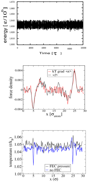
Figure 1: Top panel: Energy of a H-Adress simulation. There is practically no drift in total energy over long simulation runs (here $5\times 10^{5}\tau$, with $\tau=\sigma\sqrt{(}m/\epsilon)$ the standard Lennard-Jones time unit of the atomic potential). Middle panel: A numerical cross-check of the relation (46). Bottom panel: The temperature profile over the system. Simulations were done at density $n=0.4\sigma^{-3}$ with fitted CG-potentials.

Also, in Fig. 1 (bottom panel) the temperature profiles obtained in several type of H-AdResS simulations (with or without correction) is presented. In all cases, thermal equilibrium is attained and ensures a constant temperature profile over the simulation box. In microcanonical simulations the temperature is not an input simulation parameter so one should expect small variations in temperature upon inclusion of some form of the free energy correction (see for instance Fig. (1). In fact, a modification of the FEC term changes the overall Hamiltonian of the system and in general its second derivatives (e.g. the heat capacity) determining the caloric equation of state. For this reason, here we use a standard (canonical) thermostat while adjusting the free energy compensation in the iterative way.

VIII.2 Iterative evaluation of the free energy correction

The iterative evaluation of the free energy correction (FEC) is based on the force balance in Eq. (48), where the free energy derivative is given by Eq. (25). The virial pressure gradient in Eq. (48) stems from the inter-blob forces. Instead of evaluating its gradient, it is more efficient to use Eq. (35). We assume that the field $\lambda({\bf r})$ changes only along the $x$ axis, i.e. $\lambda({\bf r})=\lambda(x)$ and that there is translation invariance along the $y,z$ axis due to the periodic boundary conditions. This allows to average (48) with respect $y,z$. We introduce the following $x$ dependent fields

$$g(x) \equiv\langle\nabla\hat{\bm{\Pi}}_{\bf r}\cdot{\bf e}_{x}\rangle^{[\lambda]}=\left\langle\sum_{\mu\nu}\delta(\hat{X}_{\mu}-x)\hat{\bf G}_{\mu\nu}\cdot{\bf e}_{x}\right\rangle^{[\lambda]}$$

$${u}^{1}(x)-{u}^{0}(x) \equiv\left\langle\sum^{M}_{\mu}\left(V^{1}_{\mu}-V^{0}_{\mu}\right)\delta(\hat{X}_{\mu}-x)\right\rangle^{[\lambda]}$$

$$n(x) \equiv\left\langle\sum^{M}_{\mu}\delta(\hat{X}_{\mu}-x)\right\rangle^{[\lambda]}$$ (90)

The density field $a(x)$ of any microscopic quantity $A_{\mu}$ is numerically evaluated by a binned Dirac delta: $\delta_{h}(r)=\Theta_{h}(r)/V_{h}$ where $V_{h}$ is the volume of the bin and in 1D the characteristic function is $\Theta_{h}(x)=1$ if $|x|\leq h/2$ and zero otherwise. As customary we assume ergodicity and use temporal averages instead of ensemble averages

$$a(x)=\frac{1}{T_{\rm sample}}\int_{T_{\rm sample}}dt\sum_{\mu}A_{\mu}(t)\delta_{\Delta x}\left(x-x_{\mu}\right).$$ (91)

The sampling time is $T_{\rm sample}$ and the volume of the bin is $V_{\Delta x}=\Delta xL_{y}\,L_{z}$ with $L_{\alpha}$ the system’s size in $\alpha$ direction.

With the definitions (90), the mechanical equilibrium equation Eq. (48) becomes in the 1D setting

$${F_{\mathrm{c}}}(x)= \frac{u^{1}(x)-u^{0}(x)}{n(x)}\lambda^{\prime}(x)$$

$$+\frac{g(x)}{n(x)}-k_{B}T\frac{d\ln n(x)}{dx}$$ (92)

where we have introduced the “compensation” force

$${F_{\mathrm{c}}}(x)\equiv-{\cal F}^{\prime}(\lambda(x))\lambda^{\prime}(x)$$ (93)

As it is clear from Eq. (7), this is the $x$ component of the force due to the FEC acting on the atoms of the system when they have the $x$ coordinate.

Eq. (92) is valid for any form of the FEC ${\cal F}(\lambda)$ as it reflects the condition of mechanical equilibrium. The prescription to have a constant pressure field in all the system, i.e. Eq. (68), becomes in the 1D setting

$${F_{\mathrm{c}}}(x) =\frac{u^{1}(x)-u^{0}(x)}{n(x)}\lambda^{\prime}(x)$$ (94)

while the condition of constant density field, Eq. (70), becomes

$${F_{\mathrm{c}}}(x) =\frac{u^{1}(x)-u^{0}(x)}{n(x)}\lambda^{\prime}(x)+\frac{g(x)}{n(x)}$$ (95)

Note the the fields $n(x),u^{0}(x),u^{1}(x),g(x)$ depend implicitly on ${\cal F}(\lambda)$ because they are given in terms of equilibrium averages computed with a Hamiltonian that contains ${\cal F}(\lambda)$. Therefore, we need to solve (94) and (95) iteratively. The general structure of Eqs. (94),(95) is

$${F_{\mathrm{c}}}=\Phi({F_{\mathrm{c}}})$$ (96)

One way to solve this equation iteratively is

$$F_{\mathrm{c}}^{n+1}=\Phi(F_{\mathrm{c}}^{n})$$ (97)

with some initial good guess ${F_{\mathrm{c}}}^{0}$. In the present case, the Kirkwood estimate for ${\cal F}(\lambda)$ is a good guess that allows to use (97). If we do not have such a good initial estimate, we need to change the atomic forces ${F_{\mathrm{c}}}(x)$ slowly, otherwise the abrupt change in the forces on the atoms may lead to undesirable perturbations such as heat production (here we use thermostats only during the FEC calibration), density waves (that in a periodic system take a long time to be adsorbed), or even the system explosion. For this reason it is better to consider the iterative protocol

$${F_{\mathrm{c}}}^{n+1}={F_{\mathrm{c}}}^{n}+\alpha(\Phi({F_{\mathrm{c}}}^{n})-{F_{\mathrm{c}}}^{n})$$ (98)

where $\alpha$ is sufficiently small. When convergence is reached ${F_{\mathrm{c}}}^{n+1}\approx{F_{\mathrm{c}}}^{n}$ implying ${F_{\mathrm{c}}}^{n}\approx\Phi({F_{\mathrm{c}}}^{n})$. Note that $\alpha$ can be seen as the inverse of a relaxation time (the solution ideally converging exponentially fast to the converged solution, ${F_{\mathrm{c}}}^{n+1}={F_{\mathrm{c}}}^{n}$). We update Eq. (98) each sampling interval $T_{sample}=N_{s}\Delta t$ (with $N_{s}\sim 10^{3}$ time steps) and in such case $\alpha=\widehat{\alpha}\,\delta_{Kr}\left[\mathtt{mod}(n,N_{f});0\right]$, where $\delta_{Kr}$ is the Kronecker delta, $n$ is the time step, $\mathtt{mod}(n;m)$ is the modulus function and $\hat{\alpha}<1$.

The iterative solution of the constant pressure FEC equation (94) becomes now

$$F_{\mathrm{c}}^{n+1}(x) =F_{\mathrm{c}}^{n}(x)$$

$$+\alpha\left(\left[\frac{u^{1}(x)-u^{0}(x)}{n(x)}\right]^{n}\lambda^{\prime}(x)-F_{\mathrm{c}}^{n}(x)\right)$$ (99)

where the notation $[\cdots]^{n}$ means that all averages are computed with the force $F_{\mathrm{c}}^{n}(x)$ known at the $n$-th iteration.

The iterative solution of the constant density FEC equation (95) requires a further step in order to have a faster convergence rate. The idea is to first perform an iteration of the type (98)

$$F^{*}_{\mathrm{c}} =F^{n}_{\mathrm{c}}(x)+\alpha\left(\left[\frac{u^{1}(x)-u^{0}(x)}{n(x)}\right]^{n}\lambda^{\prime}(x)\right.$$

$$+\left.\left[\frac{g(x)}{n(x)}\right]^{n}-F^{n}_{\mathrm{c}}(x)\right)$$ (100)

Then, we iterate the equivalent condition $k_{B}T\nabla\ln n(x)=0$

$$F_{\mathrm{c}}^{n+1}(x) =F_{\mathrm{c}}^{n}(x)+\alpha k_{B}T\frac{d}{dx}\ln n(x)$$ (101)

which we further integrate over the hybrid layer to have

$${\cal F}^{n+1}(0) ={\cal F}^{n}(0)+\alpha k_{T}\ln\frac{n(x_{1})}{n(x_{0})}$$ (102)

where we have introduced

$${\cal F}^{n}(0) \equiv\int_{x_{0}}^{x_{1}}dxF^{n}_{\mathrm{c}}(x)$$ (103)

and finally correct the result (100) as

$$F_{\mathrm{c}}^{n+1}(x) =F_{\mathrm{c}}^{*}(x)\frac{{\cal F}^{n+1}(0)}{{\cal F}^{n}(0)}$$ (104)

The step in Eq. (102) involves the integral (103) over the transition layer so it permits to substantially reduce the fluctuations of the (total) free energy jump estimation [${\cal F}(0)$]. This fastens up the iterative evaluation of the compensation force $F_{\mathrm{c}}(x)$. An analysis of the convergence rates is however left for future work.

VIII.3 Fitted CG potentials

VIII.3.1 Kirkwood TI versus iterative evaluation of ${\cal F}$: the effect of hybrid layer width ${l}_{hyb}$.

This section analyzes the dependence of ${\cal F}(\lambda)$ on the width ${l}_{hyb}$ of the transition layer. Results will be compared with the Kirkwood thermodynamic integration ${\cal F}^{K}(\lambda)$ whose value ${\cal F}^{K}(0)$ at $\lambda=0$ is the free energy difference between both fluid models (CG and AA). Recall that by construction ${\cal F}(1)=0$, and that for fitted CG potentials, by definition of fitted, we have that ${\cal F}(0)=0$. At some $0<\lambda(x)<1$, the agreement between the Kirkwood free energy ${\cal F}^{K}(\lambda)$ and the iterative evaluation of ${\cal F}(\lambda)$ will indicate the validity of the local equilibrium approximation introduced in Sec. VII. For large enough CG and AA domains the value of ${\cal F}(0)$ has to be independent on the width of the transition layer.

The optimal result would be ${\cal F}(0)={\cal F}(0)^{K}$ for any $\lambda$, (i.e. for any width ${l}_{hyb}$). Such result would allow the H-AdResS scheme to act as a flexible and efficient tool for free energy differences evaluation. Although we will not focus here on this important thermodynamic aspect of H-AdResS , we will analyze the effect of ${l}_{hyb}$ on ${\cal F}$ by considering systems with fitted CG potentials (${\cal F}(0)={\cal F}(1)=0$) in constant pressure H-AdResS simulations. These issues will be also considered later when analyzing constant density H-AdResS under non-fitted potentials, ${\cal F}(0)\neq 0$.

The convergence of ${\cal F}^{\prime}$ is particularly fast in constant pressure simulations because it only involves averages of extensive quantities (energies). To get enough statistics for ${\cal F}^{\prime}$ in each iteration, $T_{\rm sample}$ can be chosen to be few molecular collision times. We usually started the iterative FEC evaluation using ${\cal F}(\lambda)=0$ as starting seed which is certainly a benefit, as it avoids the pre-evaluation of the Kirkwood free energy ${\cal F}^{K}$ as starting point for the iterative route. It has to be said that Molecular Dynamics H-AdResS only requires the derivative of the FEC ${\cal F}^{\prime}$ for time stepping. In this context, MD-H-AdResS Potestio et al. (2013a) offers a benefit over Monte Carlo H-AdResS Potestio et al. (2013b) because it permits to use a force balance like Eq. (94) to iteratively evaluate/update the FEC on-the-fly.

Fig. 2 compares the Kirkwood approximation to ${\cal F}$ with the iterative solution of Eq. (92) in a case with ${l}_{hyb}=5\sigma$. For large enough transition layers, molecular correlations effects lessen and we expect ${\cal F}^{\prime}$ to approach to Kirkwood’s value. To analyze how molecular correlations affect ${\cal F}^{\prime}$ we have reduced the width of the hybrid layer ${l}_{hyb}$ up to quite small values. Fig. 2 presents results for ${l}_{hyb}=2$, $2.5$ and $5\sigma$, which are similar to the molecules’ diameters (about $2.5\sigma$). Remarkably, ${\cal F^{\prime}}$ becomes quite close the Kirkwood free energy as soon as ${l}_{hyb}$ is larger than about twice the molecular cutoff radius. Maybe not unexpectedly, deviations between the iterative ${\cal F}$ and ${\cal F}^{K}$ (Kirkwood) increase around $\lambda=0$ and $\lambda=1$. Despite differences in ${\cal F}(\lambda)$, it is important to stress that for any choice of ${l}_{hyb}$ (see Fig. 2b) the iterative evaluation of ${\cal F}$ correctly predicts ${\cal F}(0)={\cal F}(1)$. We shall come back to this later in the case of non-fitted potentials.

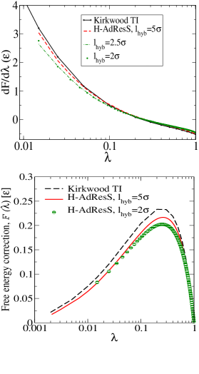
Figure 2: The derivative ${\cal F}^{\prime}$ (top) and FEC ${\cal F}(\lambda)$ (bottom) between the atomistic tetrahedral fluid and the fitted CG model as a function of $\lambda$ in constant pressure simulations. Comparison is made between the Kirkwood TI (76) and the iterative solution of Eq. (92) for several transition layer widths ${l}_{hyb}$.

Fig. 3 illustrates the effect of reducing ${l}_{hyb}$ in the density and pressure profiles in H-AdResS simulations with constant pressure. An interesting observation is that the jump of not-compensated quantities over the transition layer (here density) does not significantly increase as ${l}_{hyb}$ is made shorter. It is important to notice that in a closed system, any mass difference in the transition layer (which is a lower density region in Fig. 3) induces finite size effects. The mass excluded from the transition domain is transferred to the CG and AA domains (according to their local chemical potential) so the density in both domains will increase over the mean value $\bar{n}=M/V$ (which is indicated with a dashed line in Fig. 3a). Paradoxically, for this reason the density profile using ${l}_{hyb}=2.5\sigma$ is closer to $\bar{n}$ than the profile using from ${l}_{hyb}=5.0\sigma$ (see Fig. 3a). This mismatch in the bulk densities is reflected in the total pressure, whose (constant) value slightly depends on ${l}_{hyb}$ (see Fig. 3b).

Figure 3: The effect of reducing ${l}_{hyb}$ in the density and pressure profiles. Results corresponds to fitted CG potential at constant H-AdResS pressure.

VIII.3.2 Other finite box effects in closed systems

Fig. 4 shows the density and pressure profiles for ${l}_{hyb}=5\sigma$ in the case of fitted CG potentials. Comparison is made between simulations with ${\cal F}$ given by the pressure correction Eq. (92) and with ${\cal F}=0$. Some conclusions can be extracted. First the non-compensated version presents a larger density jump over the transition regime, when compared with the pressure compensated H-AdResS . The overall density mismatch across the transition region is slightly larger in the non-compensated H-AdResS , although it is not a large difference neither. Second, in closed boxes (here periodic) a rarefied transition region induces finite size effects on the bulk densities which become larger than $\bar{n}=M/V$. The effect is larger for ${\cal F}=0$, although this effect is observed in both simulations. This brings about consequences in the kinetic and virial pressure profiles, shown in Fig. 4b. Notably, the kinetic pressure $p^{id}=\langle k_{x}\rangle$ is equal to $k_{B}T\langle n_{x}\rangle$ (see Eq. 44) so any mismatch in density is reproduced in $p^{id}$. The total pressure $p(x)=p^{id}(x)+p^{ex}(x)$ is robustly fixed to a constant value $p(x)=P$ by the FEC. Consequently $p^{ex}$ compensates any variation in $p^{id}$ across the transition layer.

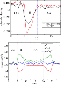
Figure 4: (a) Density profile obtained from H-AdResS with fitted CG potentials with constant pressure FEC and without FEC. (b) The kinetic $p^{id}$ and virial $p^{ex}$ contributions to the total pressure $p=p^{id}+p^{ex}$ in the pressure compensated H-AdResS with fitted CG potential. The mean pressure is $P=(1/L)\int_{0}^{L}p(x)dx$.

VIII.4 Non-fitted CG potentials

We now explore one of the main benefits of H-AdResS which is the possibility of working with non-fitted CG potentials. This benefit is not only to alleviate the time consuming and computational effort related to pre-evaluation of CG potentials. In fact, fitting the CG potential is a good practice as we have already seen that it minimizes the mismatch in non-fitted thermodynamic variables. The benefits arise from the possibility of performing simulations involving thermodynamic processes, which involve changes in the global environmental variables (temperature, pressure, chemical potential). In these cases H-AdResS permits to work with a single CG model whose ${\cal F}$ is self-adapted over the whole process to keep the desired global constraint (pressure, density, etc). In this sense H-AdResS offers an alternative to the (probably more involved) problem of potential transferability. Other benefits to be considered are the evaluation of free energies differences in systems involving large solute molecules. For these applications the estimation of the total free energy difference between (CG and AA) models should be independent on the choice of the hybrid layer and should coincide with the Kirkwood thermodynamic value. On the other hand we expect that the iterative evaluation of ${\cal F}^{\prime}$ will reduce or suppress the oscillations in the density (or pressure) profiles around the transition layer. As stated around Eq. (66), these are due to molecular correlations and have been reported in Kirkwood based pre-evaluated FEC corrections (see e.g. Potestio et al. (2013a, b)).

We start by presenting the free energy differences, pressure and density profiles obtained for the three cases considered (constant pressure and constant density FEC and no FEC) of a tetrahedral fluid facing a non-fitted CG fluid. These results are shown in Fig. 5 (FEC) and Fig. 6 (pressure and densities). Note that in this case the Kirkwood free energy ${\cal F}^{K}$ is practically equal to the constant pressure FEC correction, reflecting again the strong connection of H-AdResS with standard statistical mechanics. We will in fact hereafter focus on the constant density FEC and on its iterative evaluation. Constant density results of Fig. 5 and 6, obtained with the Kirkwood route ${\cal F}^{K}$, reveal a relatively large free energy difference between both fluids, of about ${\cal F}(0)\simeq 2.7\,k_{B}T$ per molecule. Under no-FEC contribution, this leads to substantial deviations in density and pressure across the simulation box as reflected in Fig. 6.

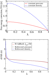
Figure 5: (Top) The FEC ${\cal F}$ evaluated from Kirkwood TI for constant pressure and constant density. (Bottom) Derivatives of Kirkwood free energies. In the constant pressure case, the H-AdResS FEC derivative ${\cal F}^{\prime}$ is compared with Kirkwood’s result. In this case, the total Helmholtz free energy difference (Kirkwood) is ${\cal F}^{K}(0)=0.85(2)$ while the iterative H-AdResS provides ${\cal F}(0)=0.86(4)$.

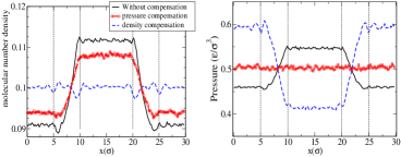
Figure 6: The density (left) and pressure (right) obtained using H-AdResS in simulations of tetrahedral molecules with the non-fitted CG potential. The corresponding FEC ${\cal F}$ is shown in Fig. 5

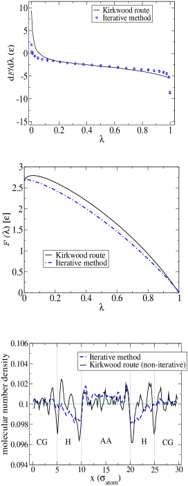
Figure 7: Free energies (top) and density profiles (bottom) for constant density H-AdResS simulations of non-fitted CG potentials. The Kirkwood free energy ${\cal F}^{K}(\lambda)$ is compared with the relaxation algorithm of Eqs. (100)-(104) for the FEC. Kirkwood total free energy jump is ${\cal F}^{K}(0)=2.67(0)$ and compares quite well with the H-AdResS iterative result ${\cal F}(0)=2.69(7)$.

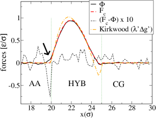
Figure 8: Details of the force balance of Eq. (95) at one of the hybrid layers of a constant density H-AdResS simulation. The iterative evaluation of ${\cal F}^{\prime}$ was performed with the algorithm of Eqs. (100)-(104) using $\Delta t=0.005$, $N_{f}=5000$ and $\hat{\alpha}=0.01$ and $\Phi=\lambda^{\prime}(x)\left(u^{1}(x)-u^{0}(x)\right)/n(x)+g(x)/n(x)$ [see Eq. (95)].

VIII.4.1 Iterative constant density FEC

Fig. 7 compares the results for ${\cal F}^{\prime}$ and ${\cal F}$ using the iterative evaluation in Eqs. (100)-(104) and the Kirkwood TI in Eq. (86) for constant density field. The first thing to highlight from Fig. 7 (top,half) is that although ${\cal F}^{\prime}(\lambda)$ (and its integral ${\cal F}(\lambda)$) differ substantially, the overall H-AdResS free energy difference ${\cal F}(0)$ results to be equal to the Kirkwood TI value. For the reasons explained before, this is an important result. Second, the density profile resulting from the iterative protocol are not completely flat, although the oscillations deviating from the mean density are softer and smaller than those obtained from Kirkwood ${\cal F}^{K}$ (maximum density deviations are $2\%$ while about $5\%$ for Kirkwood). To understand the origin of the density differences resulting from the iterative protocol (100)-(104) we plot in Fig. 8 the terms involved in the force balance over the $x$-direction. The system’s average force per molecule [RHS of Eq. 95)] is compared with the imposed compensation force ${F_{\mathrm{c}}}$. Density variations along $x$ arise with any difference between both terms; from Eq. (92), such difference is precisely $k_{B}Td\ln n/dx$ and for clarity it has been amplified by a factor 10 in Fig. 8. Indeed, ${F_{\mathrm{c}}}=0$ inside the atomistic domain but due to the small width of the transition layer and the sharp decay to zero of ${F_{\mathrm{c}}}(x)$ (particularly near $\lambda=1$, indicated with an arrow in Fig. 8) the fluid is compressed and creates density oscillations. It seems reasonable that the density oscillations are larger where the difference in compressibility is (i.e. near the atomistic border, $\lambda=1$). Fig. 8 shows that the transition of ${F_{\mathrm{c}}}$ to zero is softer at $\lambda=0$, where the density profile is also softer. These observations indicate two things: first, that density variations should eventually decrease with increasing ${l}_{hyb}$ (by allowing smaller values of $|d{F_{\mathrm{c}}}/dx|$ within the transition layer) and second, that there might also be an optimal shape of $\lambda(x)$. A study of these issues is however left for future work.

IX Conclusions

This work presented the statistical mechanics foundations of H-AdResS Potestio et al. (2013a, b). Because the method is based on a Hamiltonian, the standard techniques of Statistical Mechanics allow one to obtain a wealth of information about the thermodynamics of AA and CG models. The Hamiltonian in H-AdResS is an interpolation of the actual microscopic potential with a CG representation of the system in terms of blobs. In this way, when a blob moves from the AA region to the CG region its interactions change accordingly. We have shown why and how H-AdResS can be adapted to “connect” two different fluid models (here the atomistic and the coarse-grained models) by keeping both to coexist in the same fixed ensemble (for instance, same density or same pressure) over the same simulation box. The work required to do that is precisely the free energy compensation ${\cal F}$ which is the central ingredient of H-AdResS . We have proved that ${\cal F}(\lambda)$ is close to the free energy difference obtained from Kirkwood thermodynamic integration ${\cal F}^{K}(\lambda)$ and that both energies are equal in the limit of local thermodynamic equilibrium (in practice, wide enough transition layers). We have developed schemes to iteratively evaluate the free energy correction under either constant pressure or constant density simulations. This iterative route has several benefits. The first is a practical one, because it avoids the extra burden of implementing Kirkwood thermodynamic integration each time a FEC needs to be evaluated. Moreover, iterative evaluation of ${\cal F}$ will permit to self-adapt the FEC under a (slow enough) thermodynamic process. It is important to stress that the overall free energy jump in H-AdResS is a thermodynamic quantity which does not depend on the shape or width of the transition layer. This is confirmed by simulation results which agree withing error bars with the Kirkwood TI free energy evaluation and indeed explains the good performance of Kirkwood TI approximations to ${\cal F}$ used in Refs. Potestio et al. (2013a, b). The limits and potentiality of H-AdResS as a flexible, fast and self-adaptive free energy estimator will surely deserve further studies on denser and more disparate systems.

The emphasis in the present paper has been on equilibrium Statistical Mechanics. In order to look at problems in which dynamics is of importance, it is necessary to include the possibility in the algorithm of interpolating the full CG dynamics. In addition to the CG potential of interaction, the full CG dynamics requires the presence of friction and stochastic forces in order to fully account for eliminated degrees of freedom in the CG region Hijón et al. (2009). As it is well-known, the equilibrium properties should not be affected by the presence of these additional forces that are, however, crucial in non-equilibrium or dynamic situations. This further development is left for future work.

X Acknowledgments

We acknowledge the KAVLI Institute in Santa Barbara where this work was initiated for its hospitality and support. MINECO provided support through projects FIS2010-22047-C05-01 and FIS2010-22047-C05-03. Comunidad Autónoma de Madrid has financially supported this work through the project MODELICO.

XI Appendix: Local equilibrium in the transition layer

The exact result (65) leads to an interesting result when the typical length of variation of $\lambda({\bf r})$ is much larger than the typical length of decay of the correlations. In this case, because in the length scale in which the correlation decays, the field $\lambda({\bf r}^{\prime})$ hardly changes, we may approximate (65) by taking $\nabla\lambda({\bf r}^{\prime})\approx\nabla\lambda({\bf r})$ outside the integral as follows

$$\nabla\left\langle A_{{\bf r}}\right\rangle^{[\lambda]} \approx-\beta\nabla\lambda({\bf r})\int d{\bf r}^{\prime}\left\langle\delta A_{\bf r}(u^{1}_{{\bf r}^{\prime}}-u^{0}_{{\bf r}^{\prime}}+{\cal F}^{\prime}(\lambda({\bf r}^{\prime}))n_{{\bf r}^{\prime}})\right\rangle^{[\lambda]}$$ (105)

This approximation is equivalent to set, in Eq. (63)

$$\nabla\left\langle A_{{\bf r}}\right\rangle^{[\lambda]} \approx\nabla\lambda({\bf r})\int d{\bf r}^{\prime}\frac{\delta}{{\delta\lambda({\bf r}^{\prime})}}\left\langle A_{{\bf r}}\right\rangle^{[\lambda]}$$ (106)

Now, let us consider the average of the local function $\left\langle A_{{\bf r}}\right\rangle^{[\lambda]}$, when $\lambda({\bf r})$ changes smoothly. Consider the following rewriting of the Hamiltonian

$$H_{[\lambda]}(r,p) =H_{\lambda({\bf r})}+\delta H_{[\lambda]}$$ (107)

where we have added and subtracted a $\lambda({\bf r})$ term by defining

$$H_{\lambda({\bf r})} \equiv\sum_{i}\frac{{\bf p}_{i}^{2}}{2m_{i}}+\sum_{\mu}^{M}V^{\rm intra}_{\mu}(r)+\lambda({\bf r})\sum_{\mu}^{M}V^{1}_{\mu}(r)+(1-\lambda({\bf r}))\sum_{\mu}^{M}V^{0}_{\mu}(R)+\sum_{\mu}^{M}{\cal F}(\lambda({\bf r}))$$

$$\delta H_{[\lambda]} \equiv\sum_{\mu}^{M}(\lambda(\hat{\bf R}_{\mu})-\lambda({\bf r}))V^{1}_{\mu}(r)-\sum_{\mu}^{M}(\lambda(\hat{\bf R}_{\mu})-\lambda({\bf r}))V^{0}_{\mu}(R)+\sum_{\mu}^{M}{\cal F}(\lambda(\hat{\bf R}_{\mu}))-\sum_{\mu}^{M}\cal F(\lambda({\bf r}))$$

$$=\int d{\bf r}^{\prime}(\lambda({\bf r}^{\prime})-\lambda({\bf r}))u^{1}_{{\bf r}^{\prime}}(r)-\int d{\bf r}^{\prime}(\lambda({\bf r}^{\prime})-\lambda({\bf r}))u^{0}_{{\bf r}^{\prime}}(R)+\int d{\bf r}^{\prime}(\cal F(\lambda({\bf r}^{\prime}))-\cal F(\lambda({\bf r})))\hat{n}_{{\bf r}^{\prime}}(r)$$ (108)

Clearly, $H_{\lambda({\bf r})}$ is the Hamiltonian of a constant switching field where the value of the constant is picked to be the local value $\lambda({\bf r})$. We can now consider the average of a local function of the form

$$\langle\hat{A}_{\bf r}\rangle^{[\lambda]} =\int dz\frac{1}{Z[\lambda]}\exp\{-\beta H_{[\lambda]}\}\sum_{\mu}^{M}A_{\mu}\delta({\bf r}-{\bf R}_{\mu})$$ (109)

By expanding the exponential with respect to $\delta H_{[\lambda]}$ we have

$$\langle\hat{A}_{\bf r}\rangle^{[\lambda]} =\langle\hat{A}_{\bf r}\rangle^{\lambda=\lambda({\bf r})}+\langle\delta H_{[\lambda]}\delta\hat{A}_{\bf r}\rangle^{\lambda=\lambda({\bf r})}+\cdots$$ (110)

By using the definition (108), we have

$$\langle\delta H_{[\lambda]}\delta\hat{A}_{\bf r}\rangle^{\lambda=\lambda({\bf r})} =\int d{\bf r}^{\prime}(\lambda({\bf r}^{\prime})-\lambda({\bf r}))\langle u^{1}_{{\bf r}^{\prime}}(r)\delta\hat{A}_{\bf r}\rangle^{\lambda=\lambda({\bf r})}-\int d{\bf r}^{\prime}(\lambda({\bf r}^{\prime})-\lambda({\bf r}))\langle u^{0}_{{\bf r}^{\prime}}(R)\delta\hat{A}_{\bf r}\rangle^{\lambda=\lambda({\bf r})}$$

$$+\int d{\bf r}^{\prime}({\cal F}(\lambda({\bf r}^{\prime}))-{\cal F}(\lambda({\bf r})))\langle\hat{n}_{{\bf r}^{\prime}}(r)\delta\hat{A}_{\bf r}\rangle^{\lambda=\lambda({\bf r})}$$ (111)

It is apparent that if the switching field does not changes much on the length scale of decay of the correlations, all the above contributions may be neglected and we have

$$\langle\hat{A}_{\bf r}\rangle^{[\lambda]}\approx\langle\hat{A}_{\bf r}\rangle^{\lambda=\lambda({\bf r})}$$ (112)

This is a very natural result that tells that when the switching field does not vary appreciably in the length scale of the molecular correlations, the average of a local function in the spatially varying switching field is very well approximated with the average at a constant value of the switching field with the local value at the point ${\bf r}$ that we are considering. By using this approximation in Eq. (106), we obtain finally

$$\nabla\langle\hat{A}_{\bf r}\rangle^{[\lambda]} \approx\nabla\lambda({\bf r})\int d{\bf r}^{\prime}\frac{\delta}{{\delta\lambda({\bf r}^{\prime})}}\left\langle A_{{\bf r}}\right\rangle^{\lambda=\lambda({\bf r})}$$

$$=\nabla\lambda({\bf r})\left.\frac{d}{d\lambda}\left\langle A_{{\bf r}}\right\rangle^{\lambda}\right|_{\lambda=\lambda({\bf r})}\int d{\bf r}^{\prime}\frac{\delta\lambda({\bf r})}{{\delta\lambda({\bf r}^{\prime})}}$$

$$=\frac{d}{d\lambda}\left.\langle\hat{A}_{\bf r}\rangle^{\lambda}\right|_{\lambda=\lambda({\bf r})}\nabla\lambda({\bf r})$$ (113)

This expression allows one to express gradients of local functions as simply proportional to the gradients of the switching function whenever the switching function changes smoothly on the length scale of correlations of the CoM variables. Eq. (113) could be very roughly interpreted as a sort of “chain rule” where space derivatives are expressed in terms of derivatives with respect to the switching field. The results (72) and (113) will be referred as the local equilibrium approximation for the averages and its gradients.

XII Appendix: The force ${\bf F}_{\mu}$

In this appendix we compute explicitly the force

$$\hat{\bf F}_{\mu} =-\sum_{i}\delta_{\mu}(i)\frac{\partial}{\partial{\bf r}_{i}}\left[\sum_{\nu}V^{\rm intra}_{\nu}(r)+\sum_{\nu}\lambda(\hat{\bf R}_{\nu})V^{1}_{\nu}(r)+\sum_{\nu}(1-\lambda(\hat{\bf R}_{\nu}))V^{0}_{\nu}(R)+\sum_{\nu}{\cal F}(\lambda(\hat{\bf R}_{\nu}))\right]$$ (114)

Consider the intra potential energy of molecule $\nu$ which is defined as

$$V^{\rm intra}_{\nu}(r) =\frac{1}{2}\sum_{i^{\prime}j^{\prime}}\delta_{\nu}(i^{\prime})\delta_{\nu}(j^{\prime})\phi^{\rm intra}(r_{i^{\prime}j^{\prime}})$$ (115)

where $\phi^{\rm intra}(r_{i^{\prime}j^{\prime}})$ is the pair potential of particles $i^{\prime},j^{\prime}$ due to intramolecular interactions. Then

$$-\sum_{i}\delta_{\mu}(i)\frac{\partial}{\partial{\bf r}_{i}}\sum_{\nu}V^{\rm intra}_{\nu}(r) =-\sum_{i}\delta_{\mu}(i)\frac{\partial}{\partial{\bf r}_{i}}\sum_{\nu}\frac{1}{2}\sum_{i^{\prime}j^{\prime}}\delta_{\nu}(i^{\prime})\delta_{\nu}(j^{\prime})\phi^{\rm intra}(r_{i^{\prime}j^{\prime}})$$

$$=-\sum_{i}\delta_{\mu}(i)\sum_{\nu}\frac{1}{2}\sum_{i^{\prime}j^{\prime}}\delta_{\nu}(i^{\prime})\delta_{\nu}(j^{\prime})\frac{\partial}{\partial{\bf r}_{i}}\phi^{\rm intra}(r_{i^{\prime}j^{\prime}})$$

$$=\sum_{i}\delta_{\mu}(i)\sum_{\nu}\frac{1}{2}\sum_{i^{\prime}j^{\prime}}\delta_{\nu}(i^{\prime})\delta_{\nu}(j^{\prime})f^{\rm intra}(r_{i^{\prime}j^{\prime}}){\bf e}_{i^{\prime}j^{\prime}}(\delta_{ii^{\prime}}-\delta_{ij^{\prime}})$$

$$=\sum_{i}\delta_{\mu}(i)\sum_{\nu}\sum_{i^{\prime}j^{\prime}}\delta_{\nu}(i^{\prime})\delta_{\nu}(j^{\prime})f^{\rm intra}(r_{i^{\prime}j^{\prime}}){\bf e}_{i^{\prime}j^{\prime}}\delta_{ii^{\prime}}$$

$$=\sum_{i}\delta_{\mu}(i)\sum_{\nu}\sum_{j^{\prime}}\delta_{\nu}(i)\delta_{\nu}(j^{\prime})f^{\rm intra}(r_{ij^{\prime}}){\bf e}_{ij^{\prime}}$$

$$=\sum_{i}\sum_{\nu}\sum_{j^{\prime}}\delta_{\mu\nu}\delta_{\nu}(i)\delta_{\nu}(j^{\prime})f^{\rm intra}(r_{ij^{\prime}}){\bf e}_{ij^{\prime}}$$

$$=\sum_{ij^{\prime}}\delta_{\mu}(i)\delta_{\mu}(j^{\prime})f^{\rm intra}(r_{ij^{\prime}}){\bf e}_{ij^{\prime}}=0$$ (116)

because ${\bf e}_{ij}=-{\bf e}_{ji}$ and the indices are dummy. Indeed the total force on the molecule due to internal forces vanishes. Consider now the term

$$-\sum_{i}\delta_{\mu}(i)\frac{\partial}{\partial{\bf r}_{i}}\lambda(\hat{\bf R}_{\nu}) =-\sum_{i}\delta_{\mu}(i)\nabla\lambda(\hat{\bf R}_{\nu})\frac{\partial}{\partial{\bf r}_{i}}\sum_{i^{\prime}}\delta_{\nu}(i^{\prime})\frac{m_{i^{\prime}}}{m_{\nu}}{\bf r}_{i^{\prime}}$$

$$=-\sum_{i}\delta_{\mu}(i)\nabla\lambda(\hat{\bf R}_{\nu})\sum_{i^{\prime}}\delta_{\nu}(i^{\prime})\frac{m_{i^{\prime}}}{m_{\nu}}\delta_{ii^{\prime}}=-\nabla\lambda(\hat{\bf R}_{\nu})\delta_{\mu\nu}$$ (117)

Next, the term

$$-\sum_{i}\delta_{\mu}(i)\frac{\partial}{\partial{\bf r}_{i}}V^{1}_{\nu}(r) =-\sum_{i}\delta_{\mu}(i)\frac{\partial}{\partial{\bf r}_{i}}\frac{1}{2}\sum_{\nu^{\prime}\neq\nu}\sum_{i^{\prime}j^{\prime}}\delta_{\nu}(i^{\prime})\delta_{\nu^{\prime}}(j^{\prime})\phi^{\rm inter}(r_{i^{\prime}j^{\prime}})$$

$$=\frac{1}{2}\sum_{\nu^{\prime}\neq\nu}\sum_{ii^{\prime}j^{\prime}}\delta_{\mu}(i)\delta_{\nu}(i^{\prime})\delta_{\nu^{\prime}}(j^{\prime}){\bf F}^{1}_{i^{\prime}j^{\prime}}(\delta_{ii^{\prime}}-\delta_{ij^{\prime}})$$ (118)

where we have introduced the force ${\bf F}^{1}_{i^{\prime}j^{\prime}}$ that atom $j^{\prime}$ exerts on atom $i^{\prime}$. Therefore

$$-\sum_{i}\delta_{\mu}(i)\frac{\partial}{\partial{\bf r}_{i}}V^{\rm inter}_{\nu}(r) =\frac{1}{2}\sum_{\nu^{\prime}\neq\nu}\sum_{ij^{\prime}}\delta_{\mu}(i)\delta_{\nu}(i)\delta_{\nu^{\prime}}(j^{\prime}){\bf F}^{1}_{ij^{\prime}}-\frac{1}{2}\sum_{\nu^{\prime}\neq\nu}\sum_{ii^{\prime}}\delta_{\mu}(i)\delta_{\nu}(i^{\prime})\delta_{\nu^{\prime}}(i){\bf F}^{1}_{i^{\prime}i}$$

$$=\delta_{\mu\nu}\frac{1}{2}\sum_{\nu^{\prime}\neq\nu}\sum_{ij}\delta_{\mu}(i)\delta_{\nu^{\prime}}(j){\bf F}^{1}_{ij}-\frac{1}{2}\sum_{\nu^{\prime}\neq\nu}\delta_{\mu\nu^{\prime}}\sum_{ij}\delta_{\mu}(i)\delta_{\nu}(j){\bf F}^{1}_{ji}$$

$$=\delta_{\mu\nu}\frac{1}{2}\sum_{\nu^{\prime}\neq\nu}{\bf F}^{1}_{\mu\nu^{\prime}}+\frac{1}{2}\sum_{\nu^{\prime}\neq\nu}\delta_{\mu\nu^{\prime}}{\bf F}^{1}_{\mu\nu}$$

$$=\sum_{\nu^{\prime}\neq\nu}{\bf F}^{1}_{\nu\nu^{\prime}}(R_{\nu\nu^{\prime}})\frac{1}{2}\left[\delta_{\mu\nu}-\delta_{\mu\nu^{\prime}}\right]$$ (119)

where we have introduced the force that molecule $\mu$ exerts on molecule $\nu$ as

$${\bf F}^{1}_{\mu\nu} \equiv\sum_{ij}\delta_{\mu}(i)\delta_{\nu}(j){\bf F}^{1}_{ij}$$ (120)

Next, the term

$$-\sum_{i}\delta_{\mu}(i)\frac{\partial}{\partial{\bf r}_{i}}V^{0}_{\nu}(R) =-\sum_{i}\delta_{\mu}(i)\frac{\partial}{\partial{\bf r}_{i}}\frac{1}{2}\sum_{\nu^{\prime}}V^{0}_{\nu\nu^{\prime}}(R)$$

$$=\frac{1}{2}\sum_{\nu^{\prime}}F^{\rm cm}_{\nu\nu^{\prime}}(R_{\nu\nu^{\prime}})\sum_{i}\delta_{\mu}(i)\frac{\partial{R}_{\nu\nu^{\prime}}}{\partial{\bf r}_{i}}$$

$$=\frac{1}{2}\sum_{\nu^{\prime}}F^{\rm cm}_{\nu\nu^{\prime}}(R_{\nu\nu^{\prime}})\sum_{i}\delta_{\mu}(i)\frac{\partial{R}_{\nu\nu^{\prime}}}{\partial{\bf r}_{i}}$$ (121)

where we assumed pair-wise interactions. Then

$$\sum_{i}\delta_{\mu}(i)\frac{\partial{\bf R}_{\nu}}{\partial{\bf r}_{i}} =\sum_{i}\delta_{\mu}(i)\frac{\partial}{\partial{\bf r}_{i}}\sum_{i^{\prime}}\delta_{\nu}(i^{\prime})\frac{m_{i^{\prime}}}{m_{\nu}}{\bf r}_{i^{\prime}}$$

$$=\sum_{i}\delta_{\mu}(i)\sum_{i^{\prime}}\delta_{\nu}(i^{\prime})\frac{m_{i^{\prime}}}{m_{\nu}}{\bf 1}\delta_{ii^{\prime}}=\sum_{i}\delta_{\mu}(i)\delta_{\nu}(i)\frac{m_{i}}{m_{\nu}}{\bf 1}=\delta_{\mu\nu}{\bf 1}$$ (122)

$$\sum_{i}\delta_{\mu}(i)\frac{\partial{R}_{\nu\nu^{\prime}}}{\partial{\bf r}_{i}} ={\bf e}_{\nu\nu^{\prime}}\cdot\sum_{i}\delta_{\mu}(i)\frac{\partial{\bf R}_{\nu\nu^{\prime}}}{\partial{\bf r}_{i}}={\bf e}_{\nu\nu^{\prime}}\left[\delta_{\mu\nu}-\delta_{\mu\nu^{\prime}}\right]$$ (123)

then

$$-\sum_{i}\delta_{\mu}(i)\frac{\partial}{\partial{\bf r}_{i}}V^{0}_{\nu}(R) =\frac{1}{2}\sum_{\nu^{\prime}}F^{\rm cm}_{\nu\nu^{\prime}}(R_{\nu\nu^{\prime}})\sum_{i}\delta_{\mu}(i)\frac{\partial{R}_{\nu\nu^{\prime}}}{\partial{\bf r}_{i}}$$

$$=\frac{1}{2}\sum_{\nu^{\prime}}F^{\rm cm}_{\nu\nu^{\prime}}(R_{\nu\nu^{\prime}}){\bf e}_{\nu\nu^{\prime}}\left[\delta_{\mu\nu}-\delta_{\mu\nu^{\prime}}\right]$$

$$=\frac{1}{2}\sum_{\nu^{\prime}}{\bf F}^{0}_{\nu\nu^{\prime}}(R_{\nu\nu^{\prime}})\left[\delta_{\mu\nu}-\delta_{\mu\nu^{\prime}}\right]$$ (124)

In summary, we have

$$\hat{\bf F}_{\mu} \equiv-\sum_{i}\delta_{\mu}(i)\frac{\partial}{\partial{\bf r}_{i}}\left[\sum_{\nu}V^{\rm intra}_{\nu}(r)+\sum_{\nu}\lambda(\hat{\bf R}_{\nu})V^{\rm inter}_{\nu}(r)+\sum_{\nu}(1-\lambda(\hat{\bf R}_{\nu}))V^{0}_{\nu}(R)+\sum_{\nu}{\cal F}(\lambda(\hat{\bf R}_{\nu}))\right]$$ (125)

and have to substitute in this expression the following results

$$-\sum_{i}\delta_{\mu}(i)\frac{\partial}{\partial{\bf r}_{i}}\sum_{\nu}V^{\rm intra}_{\nu}(r) =0$$

$$-\sum_{i}\delta_{\mu}(i)\frac{\partial}{\partial{\bf r}_{i}}\lambda(\hat{\bf R}_{\nu}) =-\nabla\lambda(\hat{\bf R}_{\nu})\delta_{\mu\nu}$$

$$-\sum_{i}\delta_{\mu}(i)\frac{\partial}{\partial{\bf r}_{i}}V^{\rm inter}_{\nu}(r) =\frac{1}{2}\sum_{\nu^{\prime}}{\bf F}^{\rm intra}_{\nu\nu^{\prime}}(R_{\mu\nu^{\prime}})\left[\delta_{\mu\nu}-\delta_{\mu\nu^{\prime}}\right]$$

$$-\sum_{i}\delta_{\mu}(i)\frac{\partial}{\partial{\bf r}_{i}}V^{0}_{\nu}(R) =\frac{1}{2}\sum_{\nu^{\prime}}{\bf F}^{0}_{\nu\nu^{\prime}}(R_{\nu\nu^{\prime}})\left[\delta_{\mu\nu}-\delta_{\mu\nu^{\prime}}\right]$$ (126)

with the result

$$\hat{\bf F}_{\mu} =-\left[\sum_{\nu}\sum_{i}\delta_{\mu}(i)\frac{\partial}{\partial{\bf r}_{i}}\lambda(\hat{\bf R}_{\nu})(V^{\rm inter}_{\nu}(r)-V^{0}_{\nu}(R)-{\cal F}^{\prime}(\lambda_{\nu}(R)))\right]$$

$$-\left[\sum_{\nu}\lambda(\hat{\bf R}_{\nu})\sum_{i}\delta_{\mu}(i)\frac{\partial}{\partial{\bf r}_{i}}V^{\rm inter}_{\nu}(r)+\sum_{\nu}(1-\lambda(\hat{\bf R}_{\nu}))\sum_{i}\delta_{\mu}(i)\frac{\partial}{\partial{\bf r}_{i}}V^{0}_{\nu}(R)\right]$$

$$=-\nabla\lambda(\hat{\bf R}_{\mu})(V^{\rm inter}_{\mu}(r)-V^{0}_{\mu}(R)-{\cal F}^{\prime}(\lambda_{\mu}(R)))$$

$$+\sum_{\nu}\lambda(\hat{\bf R}_{\nu})\frac{1}{2}\sum_{\nu^{\prime}}{\bf F}^{1}_{\nu\nu^{\prime}}(R_{\mu\nu^{\prime}})\left[\delta_{\mu\nu}-\delta_{\mu\nu^{\prime}}\right]+\sum_{\nu}(1-\lambda(\hat{\bf R}_{\nu}))\frac{1}{2}\sum_{\nu^{\prime}}{\bf F}^{0}_{\nu\nu^{\prime}}(R_{\nu\nu^{\prime}})\left[\delta_{\mu\nu}-\delta_{\mu\nu^{\prime}}\right]$$

$$=-\nabla\lambda(\hat{\bf R}_{\mu})(V^{\rm inter}_{\mu}(r)-V^{0}_{\mu}(R)-{\cal F}^{\prime}(\lambda_{\mu}(R)))$$

$$+\sum_{\nu}\frac{\lambda(\hat{\bf R}_{\mu})+\lambda(\hat{\bf R}_{\nu})}{2}{\bf F}^{1}_{\mu\nu}(R_{\mu\nu})+\sum_{\nu}\left(1-\frac{\lambda(\hat{\bf R}_{\mu})+\lambda(\hat{\bf R}_{\nu})}{2}\right){\bf F}^{0}_{\nu\nu^{\prime}}(R_{\mu\nu})$$ (127)

We may introduce the following pair force

$$\hat{\bf G}_{\mu\nu} =\left[\frac{\lambda(\hat{\bf R}_{\mu})+\lambda(\hat{\bf R}_{\nu})}{2}\right]{\bf F}^{1}_{\mu\nu}(R_{\mu\nu})+\left[1-\frac{\lambda(\hat{\bf R}_{\mu})+\lambda(\hat{\bf R}_{\nu})}{2}\right]{\bf F}^{0}_{\mu\nu}(R_{\mu\nu})$$ (128)

The pair force satisfies Newton’s Third Law. With this definition we have

$$\hat{\bf F}_{\mu} =-\nabla\lambda(\hat{\bf R}_{\mu})(V^{\rm inter}_{\mu}(r)-V^{0}_{\mu}(R)-{\cal F}^{\prime}(\lambda_{\mu}(R)))+\sum_{\nu}\hat{\bf G}_{\mu\nu}$$ (129)

References

• Neri et al. (2005) M. Neri, C. Anselmi, M. Cascella, A. Maritan, and P. Carloni, Physical Review Letters 95, 218102 (2005), ISSN 0031-9007.
• Csányi et al. (2004) G. Csányi, T. Albaret, M. C. Payne, and A. De Vita, Physical review letters 93, 175503 (2004), ISSN 0031-9007.
• Voth (2009) G. A. Voth, Coarse-Graining of Condensed Phase and Biomolecular Systems (CRC Press, 2009).
• Park and Heyden (2009) J. H. Park and A. Heyden, Molecular Simulation 35, 962 (2009), ISSN 0892-7022, URL http://www.tandfonline.com/doi/abs/10.1080/08927020902902759.
• Wang et al. (2013) H. Wang, C. Hartmann, C. Schütte, and L. D. Site, Physical Review X 011018, 1 (2013).
• Potestio et al. (2013a) R. Potestio, S. Fritsch, P. Español, R. Delgado-Buscalioni, K. Kremer, R. Everaers, and D. Donadio, Phys. Rev. Lett. 110, 108301 (2013a).
• Potestio et al. (2013b) R. Potestio, P. Español, R. Delgado-Buscalioni, R. Everaers, K. Kremer, and D. Donadio, Phys. Rev. Lett. 111, 060601 (2013b).
• Ensing et al. (2007) B. Ensing, S. O. Nielsen, P. B. Moore, M. L. Klein, and M. Parrinello, Journal of Chemical Theory and Computation 3, 1100 (2007), ISSN 1549-9618.
• Nielsen et al. (2010) S. O. Nielsen, P. B. Moore, and B. Ensing, Physical Review Letters 105, 237802 (2010), ISSN 0031-9007.
• Delle Site (2007) L. Delle Site, Physical Review E 76, 047701 (2007), ISSN 1539-3755, URL http://link.aps.org/doi/10.1103/PhysRevE.76.047701.
• Praprotnik et al. (2011) M. Praprotnik, S. Poblete, L. Delle Site, and K. Kremer, Physical Review Letters 107, 099801 (2011), ISSN 0031-9007.
• Nielsen et al. (2011) S. O. Nielsen, P. B. Moore, and B. Ensing, Physical Review Letters 107, 099802 (2011), ISSN 0031-9007.
• Praprotnik et al. (2007) M. Praprotnik, L. D. Site, and K. Kremer, J. Chem. Phys 126, 134902 (2007).
• Delgado-Buscalioni et al. (2008a) R. Delgado-Buscalioni, K. Kremer, and M. Praprotnik, The Journal of chemical physics 128, 114110 (2008a), ISSN 0021-9606, URL http://www.ncbi.nlm.nih.gov/pubmed/18361557.
• Fritsch et al. (2012) S. Fritsch, S. Poblete, C. Junghans, G. Ciccotti, L. Delle Site, and K. Kremer, Phys. Rev. Lett. 108, 170602 (2012).
• Issa and Poesio (2014) K. M. Issa and P. Poesio, Phys. Rev. E 89, 043307 (2014).
• Kotsalis et al. (2007) E. M. Kotsalis, J. H. Walther, and P. Koumoutsakos, Phys. Rev. E 76, 016709 (pages 7) (2007).
• Kirkwood (1935) J. G. Kirkwood, J. Chem. Phys. 3, 300 (1935).
• Faller (2004) R. Faller, Polymer 45, 3869 (2004), ISSN 00323861.
• Shell (2008) M. S. Shell, The Journal of chemical physics 129, 144108 (2008), ISSN 1089-7690, URL http://www.ncbi.nlm.nih.gov/pubmed/19045135.
• Grabert (1982) H. Grabert, Projection Operator Techniques in Nonequilibrium Statistical Mechanics (Springer Verlag, Berlin, 1982).
• Landau and Lifshitz (1959a) L. D. Landau and E. M. Lifshitz, Fluid Mechanics (Pergamon Press, New York, 1959a).
• Frenkel and Smith (2002) D. Frenkel and B. Smith, Understanding Molecular Simulation: From Algorithms to Applications (Academic Press, San Diego, 2nd edition, 2002).
• Landau and Lifshitz (1959b) L. D. Landau and E. M. Lifshitz, Statistical Physics (Pergamon Press, 1959b).
• Praprotnik et al. (2005) M. Praprotnik, L. D. Site, and K. Kremer, J. Comp. Phys. 123, 224106 (2005).
• Delgado-Buscalioni et al. (2008b) R. Delgado-Buscalioni, K. Kremer, and M. Praprotnik, J. Chem. Phys. 128, 114110 (2008b).
• Hijón et al. (2009) C. Hijón, P. Español, E. Vanden-Eijnden, and R. Delgado-Buscalioni, Faraday Discuss. 144, 301 (2009), ISSN 1359-6640.