Critical energy density of O$(n)$ models in $d=3$

Abstract

A relation between O$(n)$ models and Ising models has been recently conjectured [L. Casetti, C. Nardini, and R. Nerattini, Phys. Rev. Lett. 106, 057208 (2011)]. Such a relation, inspired by an energy landscape analysis, implies that the microcanonical density of states of an O$(n)$ spin model on a lattice can be effectively approximated in terms of the density of states of an Ising model defined on the same lattice and with the same interactions. Were this relation exact, it would imply that the critical energy densities of all the O$(n)$ models (i.e., the average values per spin of the O$(n)$ Hamiltonians at their respective critical temperatures) should be equal to that of the corresponding Ising model; it is therefore worth investigating how different the critical energies are and how this difference depends on $n$.

We compare the critical energy densities of O$(n)$ models in three dimensions in some specific cases: the O$(1)$ or Ising model, the O$(2)$ or $XY$ model, the O$(3)$ or Heisenberg model, the O$(4)$ model and the O$(\infty)$ or spherical model, all defined on regular cubic lattices and with ferromagnetic nearest-neighbor interactions. The values of the critical energy density in the $n=2$, $n=3$, and $n=4$ cases are derived through a finite-size scaling analysis of data produced by means of Monte Carlo simulations on lattices with up to $128^{3}$ sites. For $n=2$ and $n=3$ the accuracy of previously known results has been improved. We also derive an interpolation formula showing that the difference between the critical energy densities of O$(n)$ models and that of the Ising model is smaller than $1\%$ if $n<8$ and never exceeds $3\%$ for any $n$.

I Introduction

Simple models are important tools in theoretical physics, and especially in statistical mechanics, where O$(n)$ Hamiltonians are often used to describe in highly simplified, yet significant models realistic interactions between particles or spins. Finding links or relations between different simple and paradigmatic models often results in a deeper understanding of the model themselves and of the physics they describe: from this point of view it is highly desirable to individuate and characterize exact (or even approximate) properties and quantities shared by them.

In Casetti et al. (2011) a relation between the microcanonical densities of states of continuous and discrete spin models was conjectured, and further discussed in Nardini et al. (2012, 2013). It was suggested that the density of states of an O$(n)$ classical spin model on a given lattice can be approximated in terms of the density of states of the corresponding Ising model. By “corresponding” Ising model we mean an Ising model defined on the same lattice and with the same interactions. Such a relation was inspired by an energy landscape approach Wales (2004) to the microcanonical thermodynamics of these models, the key observation being that all the configurations of an Ising model on a lattice are stationary points of an O$(n)$ model Hamiltonian defined on the same lattice with the same interactions, for any $n$. The relation between the densities of states can be written as

$$\omega^{(n)}(\varepsilon)\approx\omega^{(1)}(\varepsilon)\,g^{(n)}(\varepsilon)\,,$$ (1)

where $\varepsilon$ is the energy density of the system, i.e., $\varepsilon=E/N$ with $E$ and $N$ denoting the total energy and the number of spins, respectively; furthermore $\omega^{(n)}$ is the density of states of the O$(n)$ model, $\omega^{(1)}$ the density of states of the corresponding Ising model and $g^{(n)}$ is a function representing the volume of a neighborhood of the Ising configuration in the phase space of the O$(n)$ model. The function $g^{(n)}$ is typically unknown. However, since it comes from local integrals over a neighborhood of the phase space, one expects it is regular. Eq. (1) is an approximate one and the approximations involved are not easily controlled in general . However, as discussed in Casetti et al. (2011), were it exact there would be a very interesting consequence: the critical energy densities $\varepsilon^{(n)}_{c}$ of the phase transitions of all the O$(n)$ models on a given lattice would be the same and equal to $\varepsilon^{(1)}_{c}$, that is to the critical energy density of the corresponding Ising model.

Rather surprisingly, according to available analytical and numerical calculations the critical energy densities are indeed very close to each other whenever a phase transition is known to take place, at least for ferromagnetic models on $d$-dimensional hypercubic lattices. More precisely, the critical energy densities are the same and equal to the Ising one for all the O$(n)$ models with long-range mean-field interactions as shown by the exact solution Campa et al. (2003), and the same happens for all the O$(n)$ models on a one-dimensional lattice with nearest-neighbor interactions. Making use of the microcanonical solutions of the models, an expression analogous to (1) can be exactly computed for the mean-field and for the one-dimensional nearest-neighbors $XY$ models ($n=2$) Nardini et al. (2012): such expression implies the equality of the critical energies in the limit $\varepsilon\rightarrow\varepsilon^{(n)}_{c}$. Hence the equality of the critical energies is rooted in the expression (1) for the density of states.

In $d=2$ the critical energies of the ferromagnetic transition of the Ising model and of the Berežinskii-Kosterlitz-Thouless (BKT) transition of the $XY$ model are only slightly different, the difference being about 2% (see Ref. Casetti et al. (2011) and references therein). The thermodynamics of the two-dimensional $XY$ model has been analytically studied in Nardini et al. (2013) assuming Eq. (1) as an ansatz on the form of its density of states and then computing $g^{(2)}$ with suitable approximations. The results were compared with numerical simulations and a very good agreement was found in almost all the energy density range. This confirms the soundness of the hypotheses behind Eq.  (1) also in the two-dimensional case. It is also worth noticing that despite the difference in the nature of the Ising and of the BKT transitions in $d=2$, the two-dimensional Ising and $XY$ models share a “weak universality”: indeed, the critical exponent ratio $\beta/\nu$ and the exponent $\delta$ are equal in the two cases Archambault et al. (1997). It is tempting to think that energy landscape arguments like those discussed above may explain such a relation between the features of phase transitions so different from each other.

The very different nature, due to the Mermin-Wagner theorem, of the Ising and BKT phase transitions in two dimensions together with the fact that the comparison is between an exact result for $\varepsilon^{(1)}_{c}$ (for the Ising model) and numerical results for $\varepsilon^{(2)}_{c}$ (for the XY model) prevents the two-dimensional case from being a good test case to quantify the accuracy of the prediction on the equality of critical energy densities. From this point of view the O$(n)$ model in three dimensions ($d=3$) provides a very promising and clear-cut case study to test the equality of the critical energy densities since a phase transition occurs for all $n$ and in all cases a local order parameter becomes non-vanishing at a finite critical temperature. For nearest-neighbor interacting O$(n)$ models in $d=3$ the comparison has to be based on the outcomes of numerical simulations or on approximate methods, since no exact solution (in particular for the critical energy) exists even for the Ising case. Although typically overlooked, results reported in the literature clearly show that the critical energies measured for three-dimensional O$(n)$ spin systems with $n=1$, $2$ and $3$ are almost consistent: see Casetti et al. (2011) for a discussion on this point and de Souza and Brady Moreira (1993); Gottlob and Hasenbusch (1993); Brown and Ciftan (2006) for the critical values of the energy densities for $n=1$, $n=2$ and $n=3$, respectively.

Inspired by these results, the aim of this paper is to quantify the difference between the critical energy densities of nearest-neighbor O$(n)$ models defined on regular cubic lattices in $d=3$ and to study the dependence on $n$ of the O$(n)$ critical energy densities. This study also entails an assessment of the accuracy of the prediction of equal critical energy densities following from Eq. (1).

As shown in the following Sections, the already existing numerical estimates of the critical energy densities for three-dimensional O$(n)$ models with $n=2$ and $3$ will be improved; in the case $n=4$ we obtain a result having the same accuracy of, and in good agreement with, a very recent one given in Engels and Karsch (2012). Using these results together with the exact result for the critical energy density of the $n=\infty$ model (i.e., the spherical model Stanley (1968a)) and with the first term of the $1/n$ expansion Campostrini et al. (1996), an interpolation formula for the critical energy densities $\varepsilon^{(n)}_{c}$ will be derived, valid in the whole range $n=1,2,\ldots,\infty$. It will turn out that the difference between the critical energy densities of the O$(n)$ models and that of the corresponding Ising model is smaller than $1\%$ for O$(n)$ models with $n<8$ and never exceeds $3\%$.

The paper is organized as follows: In Sec. II the definition of O$(n)$ models is recalled and the notation used in the next Section introduced. Assuming the critical energy density of the Ising model in three dimensions known with enough accuracy Hasenbusch and Pinn (1998), in Sec. III.1 we estimate the critical energy densities of the O$(2)$, O$(3)$ and O$(4)$ models in $d=3$ via a finite-size scaling (FSS) analysis whose basic relations are presented in Sec. III.1. In Sec. III.6 the spherical model in $d=3$ is discussed since its thermodynamics is equivalent to the one of an O$(n)$ model in the $n\rightarrow\infty$ limit. The spherical model can be solved analytically in any spatial dimension $d$ and, in particular, in $d=3$: hence it provides the value of $\varepsilon^{(\infty)}_{c}$. In Sec. IV a careful comparison between the critical values of the energy densities of the above mentioned models is performed and an interpolation formula for $\varepsilon^{(n)}_{c}$ defined. Some conclusions are drawn in Sec. V.

II O$(n)$ spin models

In the following we are going to consider classical O$(n)$ spin models defined on a regular cubic lattice in $d=3$ and with periodic boundary conditions. To each lattice site $i$ an $n$-component classical spin vector $\mathbf{S}_{i}=(S_{i}^{1},\ldots,S_{i}^{n})$ of unit length is assigned. The energy of the model is given by the Hamiltonian

$$H^{(n)}=-J\sum_{\langle i,j\rangle}\mathbf{S}_{i}\cdot\mathbf{S}_{j}=-J\sum_{\langle i,j\rangle}\sum_{a=1}^{n}S^{a}_{i}S^{a}_{j}\,,$$ (2)

where the angular brackets denote a sum over all distinct pairs of nearest-neighbor lattice sites. The exchange coupling $J$ will be assumed positive, resulting in ferromagnetic interactions. The Hamiltonian (2) is globally invariant under the $O(n)$ group.

In the special cases $n=1$, $n=2$, and $n=3$, one obtains the Ising, $XY$, and Heisenberg models, respectively. The case $n=1$ is even more special because O$(1)\equiv\mathbb{Z}_{2}$ is a discrete symmetry group. In this special case the Hamiltonian (2) becomes the Ising Hamiltonian

$$H^{(1)}=-J\sum_{i,j=1}^{N}\sigma_{i}\sigma_{j}~{}\,,$$ (3)

where $\sigma_{i}=\pm 1$ $\forall i$. In all the other cases $n\geq 2$ the O$(n)$ group is continuous. Without loss of generality we shall set $J=1$ in the following (and $k_{B}=1$).

The energy density $\varepsilon=H^{(n)}/N$ lies in the energy range $[-d,d]$ where $d$ is the lattice dimension. In $d=3$ and for any $n$ the models exhibit a phase transitions at $\varepsilon=\varepsilon^{(n)}_{c}$ from a paramagnetic phase, for $\varepsilon>\varepsilon^{(n)}_{c}$, to a ferromagnetic phase, for $\varepsilon<\varepsilon^{(n)}_{c}$, with a spontaneous breaking of the O$(n)$ symmetry. The models are not exactly solvable and estimates of critical temperatures, critical exponents and other quantities at criticality have been mainly derived by means of numerical simulations, see e.g. de Souza and Brady Moreira (1993); Gottlob and Hasenbusch (1993); Brown and Ciftan (2006).

III Determination of the critical energy densities

The aim of this work is to answer the following question: what is the difference between the critical value $\varepsilon^{(n)}_{c}$ of the energy density of the O$(n)$ model (2) and the critical value $\varepsilon^{(1)}_{c}$ of the energy density of the Ising model (3)? And how does it depend on $n\in[2,\infty]$?

Some preliminary observations are necessary. As mentioned in the Introduction, three-dimensional O$(n)$ models are not exactly solvable and the value of thermodynamic functions at criticality is typically estimated numerically.

Most numerical simulations have been limited so far mostly to small $n$: see e.g. de Souza and Brady Moreira (1993); Gottlob and Hasenbusch (1993); Brown and Ciftan (2006); Engels and Karsch (2012) for $n=1$, $2$, $3$ and $4$, respectively. This is clearly understandable since these are the most relevant cases for physical applications Campostrini et al. (1996). On the other hand, different approaches like $1/n$ and strong-coupling expansions have been used for large $n$, see Ref.  Campostrini et al. (1996). The common feature of these studies is that they have been performed in the canonical ensemble. Hence, especially before the suggestion that critical energy densities might be very close or even equal Casetti et al. (2011), an accurate evaluation of the critical energy densities $\varepsilon^{(n)}_{c}$ was out of the scope of the works, and the computation of $\varepsilon^{(n)}_{c}$ was usually a byproduct of a more general task possibly focused on the determination of other parameters, such as the critical temperatures $T^{(n)}_{c}$ or the critical exponents or the free energies at the critical point. In the following we shall use Monte Carlo simulations and FSS to determine improved estimates of $\varepsilon^{(n)}_{c}$ for $n=2$ and $3$, our estimate of $\varepsilon^{(4)}_{c}$ being as accurate as the most recent in the literature Engels and Karsch (2012). The case $n=1$ has already been studied with high accuracy by Hasenbusch and Pinn in Hasenbusch and Pinn (1998) and we will simply recall their results in Sec. III.2.

The FSS analyses rely on numerical data computed by means of canonical Monte Carlo simulations using the optimized cluster algorithm spinmc for classical O$(n)$ spin models provided by the ALPS project ALP . Most of the simulations have been performed on the PLX machine at the CINECA in Casalecchio di Reno (Bologna, Italy). A small subset of the simulations has been performed with the same spinmc algorithm on the PC-farm of the Dipartimento di Fisica e Astronomia of the Università di Firenze, Italy. We typically used $5\times 10^{6}$ Monte Carlo sweeps (MCS) plus $5\times 10^{5}$ MCS of thermalization for the simulations of the O$(2)$ model and $10^{7}$ MCS plus $2.5\times 10^{6}$ MCS of thermalization for the simulations of the O$(3)$ and of the O$(4)$ model. The total cluster CPU time spent on PLX for the simulations has been more than $40000$ hours.

For each O$(n)$ model, the simulations have been performed at the value of the critical temperature $T^{(n)}_{c}$ given in the literature with an uncertainty $\varDelta T^{(n)}_{c}$. This quantity has to be taken into account in the computation of the uncertainty $\varDelta\varepsilon^{(n)}_{c}$ associated to the estimate of $\varepsilon^{(n)}_{c}$ and the uncertainty propagation procedure needs the evaluation of the critical value of the specific heat. For this reason, in the Monte Carlo simulations, besides collecting the values of the energy densities, we also computed the specific heat. The FSS procedure and the uncertainty propagation procedure will be discussed in the following section.

III.1 Finite-size scaling analysis

Let us denote by $\varepsilon^{(n)}_{c}(L)$ and $c^{(n)}(L)$ the critical values of the energy density and of the specific heat, respectively, of an O$(n)$ model defined on a regular cubic lattice of edge $L=\sqrt[3]{N}$. The relation between $\varepsilon^{(n)}_{c}(L)$ and $\varepsilon^{(n)}_{c}(\infty)\equiv\varepsilon^{(n)}_{c}$ is given by the FSS equation

$$\varepsilon^{(n)}_{c}(L)=\varepsilon^{(n)}_{c}+\varepsilon_{n}\;L^{\frac{\alpha_{n}-1}{\nu_{n}}}\,:$$ (4)

in the following we use the notation

$$D_{n}=\frac{\alpha_{n}-1}{\nu_{n}}\,.$$ (5)

An analogous expression holds for the specific heat, and it is given by

$$c^{(n)}(L)=c^{(n)}_{c}+c_{n}\;L^{\frac{\alpha_{n}}{\nu_{n}}}\,,$$ (6)

where $c^{(n)}_{c}\equiv c^{(n)}_{c}(\infty)$ denotes the critical value of the specific heat in the thermodynamic limit. In Eqs. (4) and (6), $\varepsilon_{n}$ and $c_{n}$ are model dependent fit parameters, while $\alpha_{n}$ and $\nu_{n}$ are the specific heat and the correlation length critical exponents, respectively. We do not discuss here the derivation of Eqs. (4) and (6), referring the reader to the existing literature for an in-depth analysis on the subject, see e.g. Fisher (1974); Brèzin (1982); Stanley (1999) for reviews and Schultka and Manousakis (1995) for an explicit derivation of Eqs. (4) and (6) in the case $n=2$.

For each O$(n)$ model, the estimate of the critical energy density $\varepsilon^{(n)}_{c}\pm\varDelta\varepsilon^{(n),stat}_{c}$ can be determined with a fit of the Monte Carlo data $\varepsilon^{(n)}_{c}(L)$ according to Eq. (4); here and in the following $\varDelta\varepsilon^{(n),stat}_{c}$ will denote the statistical uncertainty on $\varepsilon^{(n)}_{c}$ due to the fitting procedure.

Since our purpose is to compare the values of $\varepsilon^{(n)}_{c}$ for different $n$, any source of error in the determination of $\varDelta\varepsilon^{(n)}_{c}$ has to be considered separately. The fact that the energy data $\varepsilon^{(n)}_{c}(L)$ are computed with Monte Carlo simulations performed at $T^{(n)}_{c}$ becomes important. Indeed, the critical temperatures $T^{(n)}_{c}$ of O$(n)$ models are provided in the literature with an uncertainty $\varDelta T^{(n)}_{c}$ whose effect in the determination of $\varDelta\varepsilon^{(n)}_{c}$ has to be checked with special care. As a matter of fact, $\varDelta T^{(n)}_{c}$ can be seen as the analogous of a systematic source of error in an experimental setting; we will then denote by $\varDelta\varepsilon^{(n),syst}_{c}$ its contribution to $\varDelta\varepsilon^{(n)}_{c}$. The two contributions $\varDelta\varepsilon^{(n),stat}_{c}$ and $\varDelta\varepsilon^{(n),syst}_{c}$ to the uncertainty $\varDelta\varepsilon^{(n)}_{c}$ of $\varepsilon^{(n)}_{c}$ will be discussed separately in the following, and the final estimate of $\varepsilon^{(n)}_{c}$ will be given in the form

$$\varepsilon^{(n)}_{c}\pm\varDelta\varepsilon^{(n)}_{c}\equiv\varepsilon^{(n)}_{c}\pm\varDelta\varepsilon^{(n),stat}_{c}\pm\varDelta\varepsilon^{(n),syst}_{c}\,.$$ (7)

The systematic uncertainty $\varDelta\varepsilon^{(n),syst}_{c}$ can be estimated with two different methods. In both cases the critical value $c^{(n)}_{c}$ of the specific heat is necessary and will be computed with a fit of the Monte Carlo data $c^{(n)}_{c}(L)$ according to Eq. (6). The two methods we used to compute $\varDelta\varepsilon^{(n),syst}_{c}$ are the following:

• Method 1.

  $$\varDelta\bar{\varepsilon}^{(n),syst}_{c}=|\varepsilon^{(n)}_{c}-\bar{\varepsilon}^{(n)}_{+}|=|\varepsilon^{(n)}_{c}-\bar{\varepsilon}^{(n)}_{-}|\,:$$ (8)

  $\bar{\varepsilon}^{(n)}_{\pm}$ denote the energy densities at $T^{(n)}_{\pm}=T^{(n)}_{c}\pm\varDelta T^{(n)}_{c}$, computed with a first order Taylor expansion around $\varepsilon^{(n)}_{c}$; that is,

  $$\begin{split}\bar{\varepsilon}^{(n)}_{\pm}=&\varepsilon^{(n)}_{c}\Big{|}_{T=T^{(n)}_{c}}+\frac{d\varepsilon}{dT}\Big{|}_{T=T^{(n)}_{c}}\;\left[\left(T^{(n)}_{c}\pm\varDelta T^{(n)}_{c}\right)-T^{(n)}_{c}\right]=\\ =&\varepsilon^{(n)}_{c}\pm c^{(n)}_{c}\;\varDelta T^{(n)}_{c}\,.\end{split}$$ (9)

• Method 2.

  $$\varDelta\tilde{\varepsilon}^{(n),syst}_{c}=\cdot^{|\varepsilon^{(n)}_{c}-\tilde{\varepsilon}^{(n)}_{+}|}_{|\varepsilon^{(n)}_{c}-\tilde{\varepsilon}^{(n)}_{-}|}\,,$$ (10)

  with $\tilde{\varepsilon}^{(n)}_{\pm}$ denoting again the energy density values at $T^{(n)}_{\pm}$; at variance $\bar{\varepsilon}^{(n)}_{\pm}$, $\tilde{\varepsilon}^{(n)}_{\pm}$ are computed with a fit of the energy density data $\tilde{\varepsilon}^{(n)}_{\pm}(L)$ at $T^{(n)}_{\pm}$. The values of $\tilde{\varepsilon}^{(n)}_{\pm}(L)$ are computed in part with a first order Taylor expansion of the numerical data for $\varepsilon^{(n)}_{c}(L)$ through the relation

  $$\begin{split}\tilde{\varepsilon}^{(n)}_{\pm}(L)&=\varepsilon^{(n)}(L)\Big{|}_{T=T^{(n)}_{c}}+c^{(n)}_{c}(L)\Big{|}_{T=T^{(n)}_{c}}\left[\left(T^{(n)}_{c}\pm\varDelta T^{(n)}_{c}\right)-T^{(n)}_{c}\right]=\\ &=\varepsilon^{(n)}(L)\pm c^{(n)}_{c}(L)\;\varDelta T^{(n)}_{c}\,,\end{split}$$ (11)

  and in part —namely for $L=32$, $64$ and $128$— numerically by performing Monte Carlo simulations of the systems at $T^{(n)}_{\pm}$ (the two procedures give results for $\tilde{\varepsilon}^{(n)}_{\pm}(L)$ in excellent agreement).

  In the end, the fitting procedure is applied according to the relation

  $$\tilde{\varepsilon}^{(n)}_{\pm}(L)=\tilde{\varepsilon}^{(n)}_{\pm}+\varepsilon_{n,\pm}L^{D_{n}}$$ (12)

  with $D_{n}$ given in Eq. (5).

At the end of the analysis, $\varDelta\bar{\varepsilon}^{(n),syst}_{c}$ and $\varDelta\tilde{\varepsilon}^{(n),syst}_{c}$ will be compared and one of them will be chosen as final estimate of $\varDelta\varepsilon^{(n),syst}_{c}$.

III.2 $n=1$, the Ising model

The derivation of the critical energy density $\varepsilon^{(1)}_{c}$ for the three-dimensional Ising model can be found in Ref. Hasenbusch and Pinn (1998): the authors performed a FSS analysis of data computed with canonical Monte Carlo simulations of the system, considering lattices up to $112^{3}$ spins. The critical coupling $\beta^{(1)}_{c}\equiv 1/T^{(1)}_{c}$ reported in Hasenbusch and Pinn (1998); Talapov and Blöte (1996) is $\beta^{(1)}_{c}=0.2216544(6)$ [see as well the discussion in Landau and Binder (2009), p. 265 (Chapter 7), and references therein]. The best final estimate of the critical energy density is given by

$$\varepsilon^{(1)}_{c}\pm\varDelta\varepsilon^{(1)}_{c}=-0.99063\pm 0.00004\,.$$ (13)

The above result has been computed considering system sizes close to the maximum achievable with our tools and represents one of the most accurate estimation of $\varepsilon^{(1)}_{c}$ available in the literature (see, e.g., de Souza and Brady Moreira (1993) for a comparison). Moreover, the uncertainty $\varDelta\varepsilon^{(1)}_{c}$ in Eq. (13) has been computed combining the statistical and the systematic error as we have discussed in the previous Section. These facts led us not to repeat the analysis on the Ising model and to consider Eq. (13) as the best final estimation of $\varepsilon^{(1)}_{c}$. A further comment on this point can be found in Sec. V.

III.3 $n=2$, the XY model

We performed canonical Monte Carlo simulations of the $XY$ model defined on regular cubic lattices with edges $L=32,40,50,64,80,100$ and $128$. The simulations have been performed at a temperature $T=2.201673$ according to the critical value of the temperature $T^{(2)}_{c}=2.201673(97)$ reported in Gottlob and Hasenbusch (1993). The values for $\varepsilon^{(2)}_{c}(L)$ and $c^{(2)}_{c}(L)$ obtained from the simulations are reported in Table 1: in parentheses are the statistical errors.

Table 1: Monte Carlo results for the energy density $\varepsilon^{(2)}_{c}(L)$ and for the specific heat $c^{(2)}_{c}(L)$ at the critical temperature $T^{(2)}_{c}=2.201673$.

$L$	$\varepsilon^{(2)}_{c}(L)$	$c^{(2)}_{c}(L)$
32	-0.9982(3)	2.611(31)
40	-0.99589(12)	2.709(18)
50	-0.99382(9)	2.825(24)
64	-0.99233(14)	2.923(59)
80	-0.99137(6)	3.074(34)
100	-0.99067(4)	3.199(38)
128	-0.99020(4)	3.282(54)

We fitted the energy density data reported in Table 1 according to the relation (4) considering different choices for the critical exponents. In particular we chose: (i) the experimental values $\nu_{2}=0.6705(6)$ and $\alpha_{2}=-0.0115(18)$ as reported in Goldner and Ahlers (1992); (ii) $\nu_{2}=0.662(7)$ obtained in Gottlob and Hasenbusch (1993) at the same critical value of the temperature as in our case and $\alpha_{2}=-0.014(21)$ as derived from the scaling relation $\alpha_{2}=2-d\nu_{2}$ with $d=3$; (iii) $\nu_{2}=0.6723(3)$ obtained in Hasenbusch and Török (1999) with a high statistics simulation performed at a slightly different value of the temperature and $\alpha_{2}=-0.017(3)$ as derived from the scaling relation $\alpha=2-d\nu$ with $d=3$; (iv) $\alpha_{2}/\nu_{2}=-0.0258(75)$ and $1/\nu_{2}=1.487(81)$ as obtained in Schultka and Manousakis (1995) with a similar analysis. The results of the fits for $\varepsilon^{(2)}_{c}$ and for the fitting parameter $\varepsilon_{2}$ are reported in Table 2. We also performed a four-parameters fit considering $\alpha_{2}$, $\nu_{2}$, $\varepsilon^{(2)}_{c}$ and $\varepsilon_{2}$ as free parameters. However, no meaningful results could be extracted from the fit, the relative error on the parameters being larger than $100\%$ on the critical exponents (data not shown).

Table 2: Fitting values of the parameters $\varepsilon^{(2)}_{c}$ and $\varepsilon_{2}$ entering expression (4).

Fitting parameters	$\nu_{2}$ and $\alpha_{2}$	results	$\chi^{2}/\text{d.o.f.}$
	$\nu_{2}=0.6705$	$\varepsilon^{(2)}_{c}=-0.98900(3)$
$\varepsilon^{(2)}_{c},\;\varepsilon_{2}$	$\alpha_{2}=-0.0115$	$\varepsilon_{2}=-1.77(2)$	$0.60$
	$\nu_{2}=0.662$	$\varepsilon^{(2)}_{c}=-0.98904(3)$
$\varepsilon^{(2)}_{c},\;\varepsilon_{2}$	$\alpha_{2}=-0.014$	$\varepsilon_{2}=-1.92(2)$	$0.57$
	$\nu_{2}=0.6723$	$\varepsilon^{(2)}_{c}=-0.98901(3)$
$\varepsilon^{(2)}_{c},\;\varepsilon_{2}$	$\alpha_{2}=-0.017$	$\varepsilon_{2}=-1.79(2)$	$0.59$
	$\alpha_{2}/\nu_{2}=-0.0258$	$\varepsilon^{(2)}_{c}=-0.98901(3)$
$\varepsilon^{(2)}_{c},\;\varepsilon_{2}$	$1/\nu_{2}=1.487$	$\varepsilon_{2}=-1.79(2)$	$0.59$

All the results reported in Table 2 have a $\chi^{2}/\text{d.o.f.}\simeq 0.6$ and all the values of the critical energy densities $\varepsilon^{(2)}_{c}$ are consistent with each other. This fact implies that $\varepsilon^{(2)}_{c}$ is rather insensitive to the choice of the critical exponents $\nu_{2}$ and $\alpha_{2}$ (and so to the values of the critical temperatures at which they have been computed). Anyway, as best estimate of the fitting parameters we chose:

$$\begin{split}\varepsilon^{(2)}_{c}\pm\varDelta\varepsilon^{(2),stat}_{c}&=-0.98904\;\pm\;0.00003\,,\\ \varepsilon_{2}&=-1.92\;\pm\;0.02\end{split}$$ (14)

reported in the second row of Table 2. These values correspond to a choice of the critical exponents given by $\nu_{2}=0.662$ and $\alpha_{2}=-0.014$ as derived in Gottlob and Hasenbusch (1993) (second raw of Table 2) assuming the same value of $T^{(2)}_{c}$ as in our case. The curve $\varepsilon^{(2)}_{c}(L)$ given by Eq. (4) for $n=2$ and with the values of $\varepsilon^{(2)}_{c}$ and $\varepsilon_{2}$ as in Eq. (14) is shown in Fig. 1 together with the simulation data. $\varepsilon^{(2)}_{c}$ and $\varepsilon_{2}$ in Eq. (14) are consistent with the values reported in Schultka and Manousakis (1995); therein, authors found $\varepsilon^{(2)}_{c}=-0.9890(4)$ and $\varepsilon_{2}=-1.81(38)$. It is worth noticing that our result $\varepsilon^{(2)}_{c}=-0.98904(3)$ given in Eq. (14) has one digit of precision more than previous results obtained with analogous techniques, see e.g. Schultka and Manousakis (1995).

We fitted data of $c^{(2)}_{c}(L)$ reported in Table 1 according to the scaling relation given in Eq. (6) and keeping the value of the ratio $\alpha_{2}/\nu_{2}$ constant and equal to $\alpha_{2}/\nu_{2}=-0.02$, as given in Gottlob and Hasenbusch (1993). The result of the fit is reported in the first row of Table 3. To check the dependence of the specific heat on the value of the ratio $\alpha_{2}/\nu_{2}$, we also performed the same fit for different values of the critical exponents: (i) $\alpha_{2}/\nu_{2}=-0.0285$ as reported in Schultka and Manousakis (1995); (ii) $\alpha_{2}/\nu_{2}=-0.025$ as obtained from data in Hasenbusch and Török (1999); (iii) $\alpha_{2}/\nu_{2}=-0.0172$ as obtained from the experimental values of the critical exponents reported in Goldner and Ahlers (1992). The results of the fits for $c^{(2)}_{c}$ and $c_{2}$ with these choices of the critical exponents are reported in the second, third and fourth row of Table 3, respectively.

Although the values of $c^{(2)}_{c}$ reported in Table 3 are not all consistent with each other, the results in the first three rows are comparable. Moreover, our results assuming $\alpha_{2}/\nu_{2}=-0.0285$ are in agreement with the results computed in Schultka and Manousakis (1995) with the same choice of the ratio of the critical exponents. Indeed, authors found $c^{(2)}_{c}=20.45(66)$ and $c_{2}=-19.61(72)$ with a fit based on data derived form Monte Carlo simulations at a different value of the critical temperature. Interestingly the values of the fitting parameters $c^{(2)}_{c}$ and $c_{2}$ are slightly larger when the experimentally determined critical exponents $\nu_{2}=0.6705$ and $\alpha_{2}=-0.0115$ Goldner and Ahlers (1992) are considered, see the last row of Table 3. This fact was already pointed out in Schultka and Manousakis (1995) where the authors found $c^{(2)}_{c}=30.3\pm 1.0$ and $c_{2}=-29.4\pm 1.1$ for the same choice of the critical exponents. These results suggest that the value of $c^{(2)}_{c}$ strongly depends on the value of the ratio $\alpha_{2}/\nu_{2}$. In Schultka and Manousakis (1995) the authors considered lattice sizes up to $L=80$ and suggested that a wider range of lattice sizes should be necessary to determine the asymptotic value of $c^{(2)}_{c}$. In our analysis we considered lattice sizes up to $L=128$, giving $N$ almost $4$ times bigger than in Schultka and Manousakis (1995), but the discrepancy is still visible. Lattice sizes bigger than $128^{3}$ spins may be needed to improve the estimate of $c^{(2)}_{c}$. For our purposes, we can consider

$$\begin{split}c^{(2)}_{c}\pm\varDelta c^{(2)}_{c}&=28.4\pm 0.6\,,\\ c_{2}&=-27.7\pm 0.7\end{split}$$ (15)

as best final estimates of the fitting parameters. These quantities, in fact, derive from the fit with $\alpha_{2}/\nu_{2}=-0.02$ as obtained in Gottlob and Hasenbusch (1993) assuming the same value of the critical temperature $T^{(2)}_{c}=2.201673$ as in our case. We refer the reader to Schultka and Manousakis (1995) for a more detailed discussion of this problem.

Table 3: Fitting values of the parameters $c^{(2)}_{c}$ and $c_{2}$ entering expression (6).

Fitting parameters	$\alpha_{2}/\nu_{2}$	results	$\chi^{2}/\text{d.o.f.}$
		$c^{(2)}_{c}=28.4\pm 0.6$
$c^{(2)}_{c},\;c_{2}$	$\alpha_{2}/\nu_{2}=-0.02$	$c_{2}=-27.7\pm 0.7$	$0.2$
		$c^{(2)}_{c}=22.7\pm 0.5$
$c^{(2)}_{c},\;c_{2}$	$\alpha_{2}/\nu_{2}=-0.0258$	$c_{2}=-21.9\pm 0.5$	$0.2$
		$c^{(2)}_{c}=23.3\pm 0.5$
$c^{(2)}_{c},\;c_{2}$	$\alpha_{2}/\nu_{2}=-0.025$	$c_{2}=-22.6\pm 0.6$	$0.2$
		$c^{(2)}_{c}=32.5\pm 0.7$
$c^{(2)}_{c},\;c_{2}$	$\alpha_{2}/\nu_{2}=-0.0172$	$c_{2}=-31.8\pm 0.8$	$0.2$

The curve $c^{(2)}_{c}(L)$ given by Eq. (6) for $n=2$ with $c^{(2)}_{c}$ and $c_{2}$ as in Eq. (15) is plotted in Fig. 2 together with the simulation data.

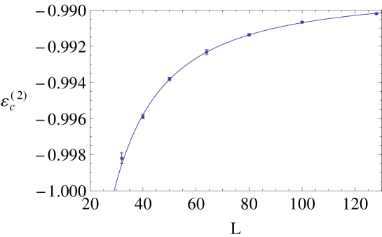
Figure 1: Energy density $\varepsilon^{(2)}_{c}$ at the critical temperature $T^{(2)}_{c}=2.201673$ as a function of $L$. The solid curve is the fit to (14) with $\nu_{2}=0.662$ and $\alpha_{2}=-0.014$.

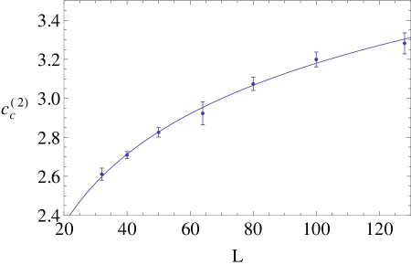
Figure 2: Specific heat $c^{(2)}_{c}$ at the critical temperature $T^{(2)}_{c}=2.201673$ as a function of $L$. The solid curve represents the fit to (15) with $\alpha_{2}/\nu_{2}=-0.02$.

In order to evaluate the systematic contribution to the uncertainty, $\varDelta\varepsilon^{(2),syst}_{c}$, we applied the two methods presented in Sec. III.1.

• Method 1. From Eq. (9), we computed $\bar{\varepsilon}^{(2)}_{+}$ and $\bar{\varepsilon}^{(2)}_{-}$ at $T^{(2)}_{+}=2.20177$ and $T^{(2)}_{-}=2.201576$, respectively, assuming $\varepsilon^{(2)}_{c}=-0.98904$ as reported in Eq. (14). These quantities are given by $\bar{\varepsilon}^{(2)}_{+}=-0.98629$ and $\bar{\varepsilon}^{(2)}_{-}=-0.99180$ and are such that $|\varepsilon^{(2)}_{c}-\bar{\varepsilon}^{(2)}_{+}|=|\varepsilon^{(2)}_{c}-\bar{\varepsilon}^{(2)}_{-}|\simeq 0.003$. In this way, we get

  $$\varDelta\bar{\varepsilon}^{(2),syst}_{c}=|\varepsilon^{(2)}_{c}-\bar{\varepsilon}^{(2)}_{\pm}|=0.003.$$ (16)

• Method 2. We computed $\tilde{\varepsilon}^{(2)}_{\pm}$ with a fit of the energy density data $\tilde{\varepsilon}^{(2)}_{\pm}(L)$ for $L=40,50,80$ and $100$ at $T^{(2)}_{+}=2.20177$ and $T^{(2)}_{-}=2.201576$, respectively, according to Eq. (12) with $n=2$ and $D_{2}=-1.5317$ as derived from data in Gottlob and Hasenbusch (1993). $\tilde{\varepsilon}^{(2)}_{\pm}(L)$ for these values of $L$ are computed with Eq. (11) from data given in Table 1. For some particular values of $L$, namely for $L=32,64$ and $128$, we performed Monte Carlo simulations at $T^{(2)}_{+}$ and $T^{(2)}_{-}$, respectively, to compute the numerical values $\mathbf{\varepsilon}^{(2)}_{\pm}(32)$, $\mathbf{\varepsilon}^{(2)}_{\pm}(64)$ and $\mathbf{\varepsilon}^{(2)}_{\pm}(128)$. The numerical results have been compared with the same quantities as derived with the Taylor expansion (11) and appeared to be consistent with them. This result reinforce the robustness of the analytical procedure used to derive $\varDelta\tilde{\varepsilon}^{(2),syst}_{c}$ and we considered the simulation values $\mathbf{\varepsilon}^{(2)}_{\pm}(32)$, $\mathbf{\varepsilon}^{(2)}_{\pm}(64)$ and $\mathbf{\varepsilon}^{(2)}_{\pm}(128)$ in the fitting procedure for the derivation of $\tilde{\varepsilon}^{(2)}_{\pm}$. The data used in the analysis are given in Table 4 in which data derived from Monte Carlo simulations are in bold and data derived with the Taylor expansion (11) are in plain text. The result of the fits are reported in Table 5; we get

  $$\varDelta\tilde{\varepsilon}^{(2),syst}_{c}=\cdot^{|\varepsilon^{(2)}_{c}-\tilde{\varepsilon}^{(2)}_{+}|}_{|\varepsilon^{(2)}_{c}-\varepsilon^{(2)}_{-}|}=\cdot^{+0.0003}_{-0.0003}=0.0003\,.$$ (17)

Table 4: Energy density data $\varepsilon^{(2)}_{+}$ and $\varepsilon^{(2)}_{-}$ obtained via Taylor expansion and numerical Monte Carlo simulations (bold), at $T^{(2)}_{+}=2.20177$ and $T^{(2)}_{-}=2.201576$, respectively.

$L$	$\varepsilon^{(2)}_{+}(L)$	$\varepsilon^{(2)}_{-}(L)$
32	-0.99854(15)	-0.9984(3)
40	-0.99563(12)	-0.99615(12)
50	-0.99355(9)	-0.99409(9)
64	-0.99197(7)	-0.99270(7)
80	-0.99107(6)	-0.99167(6)
100	-0.99036(4)	-0.99098(4)
128	-0.98994(4)	-0.99049(4)

Table 5: Fitting values of the parameters $\varepsilon^{(2)}_{\pm}$ and $\varepsilon^{(2)}_{\pm}$. In parentheses are the statistical errors due to the fitting procedure.

Fitting parameters	constants	results	$\chi^{2}/\text{d.o.f.}$
		$\varepsilon^{(2)}_{+}=-0.98871(5)$
$\varepsilon^{(2)}_{+},\;\varepsilon_{2,+}$	$D_{2}=-1.5317$	$\varepsilon_{2,+}=-1.95(3)$	$1.46$
		$\varepsilon^{(2)}_{-}=-0.98935(4)$
$\varepsilon^{(2)}_{-},\;\varepsilon_{2,-}$	$D_{2}=-1.5317$	$\varepsilon_{2,-}=-1.91(3)$	$0.8$

In Sec. IV we are going to compare the critical values of the energy density of different O$(n)$ models both in the limit of small $n$ and in the limit $n\rightarrow\infty$; we should then consider $\varDelta\varepsilon^{(2),syst}_{c}=\varDelta\bar{\varepsilon}^{(2),syst}_{c}$ given in Eq. (16), being the largest among the two different estimations of the systematic uncertainties reported in Eqs. (16) and (17), respectively. However, this result depends on the value of $c^{(2)}_{c}$ given in Eq. (15) that, in turn, is strongly affected by the choice of the ratio $\alpha_{2}/\nu_{2}$. For this reason we prefer to consider $\varDelta\tilde{\varepsilon}^{(2),syst}_{c}$ given in Eq. (17) as best estimate of $\varDelta\varepsilon^{(2),syst}_{c}$. We finally have

$$\varepsilon^{(2)}_{c}\pm\varDelta\varepsilon^{(2),stat}_{c}\pm\varDelta\varepsilon^{(2),syst}_{c}=-0.98904\;\pm\;0.00003\;\pm\;0.0003$$ (18)

as final best estimate for the critical energy density of the O$(2)$ model in three dimensions. The uncertainty $\varDelta\varepsilon^{(2),syst}_{c}$ due to $\varDelta T^{(2)}_{c}$ is an order of magnitude larger than the statistical error: this feature will be in common with all the other models considered.

III.4 $n=3$, the Heisenberg model

We performed canonical Monte Carlo simulations of the Heisenberg model defined on a regular cubic lattices with edges $L=32,40,50,64,80,100$ and $128$. As best estimate of the critical temperature of the system we considered the value $T^{(3)}_{c}=1.44298(2)$ given in Brown and Ciftan (2006). The values for $\varepsilon^{(3)}_{c}(L)$ and $c^{(3)}_{c}(L)$ obtained from the simulations are reported in Table 6: in parentheses are the statistical errors.

Table 6: Monte Carlo results for the energy density $\varepsilon^{(3)}_{c})$ and for the specific heat $c^{(2)}_{c}$ at the critical temperature $T^{(3)}_{c}=1.44298$.

$L$	$\varepsilon^{(3)}_{c}(L)$	$c^{(3)}_{c}(L)$
32	-0.99646(7)	2.863(15)
40	-0.99437(6)	2.938(19)
50	-0.99289(5)	3.030(19)
64	-0.99183(4)	3.126(23)
80	-0.99116(3)	3.197(28)
100	-0.99064(3)	3.259(32)
128	-0.990312(14)	3.367(28)

We fitted data reported in Table 6 according to relation (4) with $n=3$ and considering $\varepsilon^{(3)}_{c}$ and $\varepsilon_{3}$ as fitting parameters. For the values of the critical exponents, we considered different choices: (i) the best theoretical estimates $\nu_{3}=0.705(3)$ and $\alpha_{3}=-0.115(9)$ coming from a re-summed perturbation series analysis Le Guillou and Zinn-Justin (1980); (ii) we used $\alpha_{3}-1)/\nu_{3}=-1.586(19)$ as obtained in Holm and Janke (1994) from a similar analysis performed using a slightly different value of the critical temperature, namely $T_{c}=1.4430$; (iii) we considered $(\alpha_{3}-1)/\nu_{3}=-1.5974$ as derived in Brown and Ciftan (2006) from a similar analysis performed using t he same value of $T^{(3)}_{c}$ as in our case. The results of these fits for $\varepsilon^{(3)}_{c}$ and $\varepsilon_{3}$ are reported in Table 7.

Table 7: Fitting values of the parameters $\varepsilon^{(3)}_{c}$ and $\varepsilon_{3}$ entering expression (4).

Fitting parameters	$\nu_{3}$ and $\alpha_{3}$	results	$\chi^{2}/\text{d.o.f.}$
	$\nu_{3}=0.705$	$\varepsilon^{(3)}_{c}=-0.989537(12)$
$\varepsilon^{(3)}_{c},\;\varepsilon_{3}$	$\alpha_{3}=-0.115$	$\varepsilon_{3}=-1.652(10)$	$0.52$
		$\varepsilon^{(3)}_{c}=-0.989542(11)$
$\varepsilon^{(3)}_{c},\;\varepsilon_{3}$	$D_{3}=-1.586$	$\varepsilon_{3}=-1.677(10)$	$0.48$
		$\varepsilon^{(3)}_{c}=-0.989556(10)$
$\varepsilon^{(3)}_{c},\;\varepsilon_{3}$	$D_{3}=-1.5974$	$\varepsilon_{3}=-1.744(9)$	$0.40$

We also performed a fit of all the parameters $\varepsilon^{(3)}_{c}$, $\varepsilon_{3}$ and $D_{3}=(\alpha_{3}-1)/\nu_{3}$ with the scaling relation $\varepsilon^{(3)}_{c}(L)=\varepsilon^{(3)}_{c}+\varepsilon_{3}L^{D_{3}}$. The results are $\varepsilon^{(3)}_{c}=-0.98958(3)$, $\varepsilon_{3}=-1.88(17)$ and $D_{3}=-1.62(2)$ with a $\chi^{2}/\text{d.o.f.}\simeq 0.43$. These results are in agreement with those reported in Table 7 and with the results reported in literature, see e.g. Holm and Janke (1994); Brown and Ciftan (2006). However, as they come from a three-parameters fit of a relatively small set of data, we chose to neglect them and to consider only results reported in Table 7 in our study.

The values of the parameters reported in the second row of Table 7 are consistent with the corresponding quantities reported in Holm and Janke (1994). Therein, the authors obtain $\varepsilon^{(3)}_{c}=-0.9894(1)$, $\varepsilon_{3}=-1.68(8)$ and $D_{3}=-1.586(19)$. These values come from a three parameter fit of the scaling relation $\varepsilon^{(3)}_{c}(L)=\varepsilon^{(3)}_{c}+\varepsilon_{3}L^{D_{3}}$ with $D_{3}=(\alpha_{3}-1)/\nu_{3}$, performed at $T_{c}=1.4430\neq T^{(3)}_{c}$. Beside supporting our results, this fact seems to suggest that $\varepsilon^{(3)}_{c}$ does not sensibly depend on the value of the critical temperature.

For what concerns the third row of Table 7, the results of the fit have to be compared with the results computed in Brown and Ciftan (2006) at the same value of $T^{(3)}_{c}$ as in our case. Therein, the authors find

$$\varepsilon^{(3)}_{c}(L)=\varepsilon^{(3)}_{c}+\varepsilon_{3}L^{D_{3}}=-0.9896\pm 1.7225L^{-1.5974}\,;$$ (19)

the relative precision of the data fit being of $0.001\%$ or better. Also in this case our results, obtained for $D_{3}=-1.5974$, are perfectly consistent.

The values of the parameter $\varepsilon^{(3)}_{c}$ reported in Table 7 are consistent with each other. The results reported in the third row of Table 7 have been determined considering a combination of the critical exponents $D_{3}$ as derived in Brown and Ciftan (2006) at the same value of the critical temperature as in our case. Since the numerical value of $\alpha_{3}/\nu_{3}$ is needed in the following to determine $c^{(3)}_{c}$, we give

$$\begin{split}\varepsilon^{(3)}_{c}\;\pm\;\varDelta\varepsilon^{(3),stat}_{c}&=-0.989556\;\pm\;0.000010\,,\\ \varepsilon_{3}&=-1.744\;\pm\;0.009\,;\end{split}$$ (20)

as best estimate of the critical energy density value of $\varepsilon^{(3)}_{c}$. The curve $\varepsilon^{(3)}_{c}(L)$ given by Eq. (4) for $n=3$ and with the values of $\varepsilon^{(3)}_{c}$ and $\varepsilon_{3}$ as in Eq. (20) is shown in Fig. 3 together with the simulation data. It is worth noticing that the value of $\varepsilon^{(3)}_{c}$ in Eq. (20) is given with one digit of precision more than previous results in the literature and obtained with similar techniques Holm and Janke (1994); Brown and Ciftan (2006).

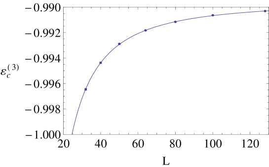
Figure 3: Energy density $\varepsilon^{(3)}_{c}$ at the critical temperature $T^{(3)}_{c}=1.4498$ as a function of $L$. The solid curve is the fit to (20) with $(\alpha_{3}-1)/\nu_{3}=-1.5974$.

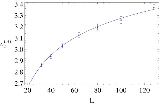
Figure 4: Specific heat $c^{(3)}_{c}$ at the critical temperature $T^{(3)}_{c}=1.4498$ as a function of $L$. The solid curve is the fit to (21) with $\alpha_{3}/\nu_{3}=-0.1991$.

We fitted data of $c^{(3)}_{c}(L)$ reported in Table 6 according to the scaling relation given in Eq. (6) with $\alpha_{3}/\nu_{3}=-0.1991$ as in Brown and Ciftan (2006). The results of the fit are reported in the first row of Table 8. To check the dependence of our results from the ratio $\alpha_{3}/\nu_{3}$ we performed the same fit for two different choices of $\alpha_{3}/\nu_{3}$: (i) $\alpha_{3}/\nu_{3}=-0.1631$ as derived in Le Guillou and Zinn-Justin (1980) and (ii) $\alpha_{3}/\nu_{3}=-0.166$ as derived in Holm and Janke (1994). The results of these fits are reported in the second and third rows of Table 8, respectively. We chose

$$\begin{split}c^{(3)}_{c}&=4.91\;\pm\;0.03\,,\\ c_{3}&=-4.09\;\pm\;0.09\,;\end{split}$$ (21)

as the best choice of the fitting parameters, being associated to a choice of the critical exponents as in Brown and Ciftan (2006) at the same value of $T^{(3)}_{3}$ as in our case. The curve $c^{(3)}_{c}(L)$ given by Eq. (6) for $n=3$ and the values of the fitting parameters $c^{(3)}_{c}$ and $c_{3}$ as in Eq. (21) is shown in Fig. 4 together with the simulation data.

Table 8: Fitting values of the parameters $c^{(3)}_{c}$ and $c_{3}$ entering expression (4) with $n=3$.

Fitting parameters	constants	results	$\chi^{2}/\text{d.o.f.}$
		$c^{(3)}_{c}=4.91(3)$
$c^{(3)}_{c},\;c_{3}$	$\alpha_{3}/\nu_{3}=-0.1991$	$c_{2}=-4.09(9)$	$0.18$
		$c^{(3)}_{c}=5.31(5)$
$c^{(3)}_{c},\;c_{3}$	$\alpha_{3}/\nu_{3}=-0.1631$	$c_{3}=-4.32(8)$	$0.15$
		$c^{(3)}_{c}=5.27(4)$
$c^{(3)}_{c},\;c_{3}$	$\alpha_{3}/\nu_{3}=-0.166$	$c_{3}=-4.29(8)$	$0.15$

In order to evaluate $\varDelta\varepsilon^{(3),syst}_{c}$, we applied the two methods presented in Sec. III.1 specialized to $n=3$:

• Method 1. From Eq. (9) we computed the values of $\bar{\varepsilon}^{(3)}_{+}$ and $\bar{\varepsilon}^{(3)}_{-}$ at $T^{(3)}_{+}=1.44300$ and $T^{(3)}_{-}=1.44296$, respectively, assuming $\varepsilon^{(3)}_{c}=-0.989556$ as reported in Eq.  (20). These quantities are given by $\bar{\varepsilon}^{(3)}_{+}=-0.989458$ and $\bar{\varepsilon}^{(3)}_{-}=-0.989654$ and are such that $|\varepsilon^{(3)}_{c}-\bar{\varepsilon}^{(3)}_{+}|=|\varepsilon^{(3)}_{c}-\bar{\varepsilon}^{(3)}_{-}|\simeq 0.00010$. In this way, we get

  $$\varDelta\bar{\varepsilon}^{(3),syst}_{c}=|\varepsilon^{(3)}_{c}-\bar{\varepsilon}^{(3)}_{\pm}|=0.00010.$$ (22)

• Method 2. We computed $\tilde{\varepsilon}^{(3)}_{\pm}$ with a fit of the energy density data for $\tilde{\varepsilon}^{(3)}_{\pm}(L)$ for $L=32,40,50,64,80,100$ and $128$ at $T^{(3)}_{+}=1.44300$ and $T^{(3)}_{-}=1.44296$, respectively, according to Eq. (12) with $n=3$ and $D_{3}=-1.5974$ as in Brown and Ciftan (2006). For $L=40,50,80,100$ we computed $\tilde{\varepsilon}^{(3)}_{\pm}(L)$ by applying Eq. (11) to data given in Table 6. As in the case of the $XY$ model, the values of $\tilde{\varepsilon}^{(3)}_{\pm}(L)$ for $L=32,64$ and $128$ are obtained with Monte Carlo simulations performed at $T^{(3)}_{+}$ and $T^{(3)}_{-}$, respectively; these numerical values are consistent with the same quantities computed with Eq. (11), not shown here. The data involved in the analysis are shown in Table 9; data arising from the Monte Carlo simulations are printed in bold and data computed using Eq. (11) are printed in plain text. From the fits we get

  $$\varDelta\tilde{\varepsilon}^{(3),syst}_{c}=\cdot^{|\varepsilon^{(3)}_{+}-\varepsilon^{(3)}_{c}|}_{|\varepsilon^{(3)}_{-}-\varepsilon^{(3)}_{c}|}=\cdot^{+0.00008}_{-0.00006}$$ (23)

as reported in Table 10. Since our purpose is to compare the values of the critical energy density for different O$(n)$ models, we choose $\varDelta\bar{\varepsilon}^{(3),syst}_{c}$ in Eq. (22) as best estimate of the systematic uncertainty on $\varepsilon^{(3)}_{c}$. From Eqs. (20) and (22) we finally get

$$\varepsilon^{(3)}_{c}\;\pm\;\varDelta\varepsilon^{(3),stat}_{c}\;\pm\;\varDelta\varepsilon^{(3),syst}_{c}=-0.989556\;\pm\;0.000010\;\pm\;0.00010,$$ (24)

as best estimate of the critical energy density of the three dimensional Heisenberg model, in the thermodynamic limit.

Table 9: Energy density data $\varepsilon^{(3)}_{+}(L)$ and $\varepsilon^{(3)}_{-}(L)$ obtained via Taylor expansion (plain text) and numerical Monte Carlo simulations (bold), at $T^{(3)}_{+}=1.44300$ and $T^{(3)}_{-}=1.44296$, respectively. The statistical errors are in parentheses.

$L$	$\varepsilon^{(3)}_{+}(L)$	$\varepsilon^{(3)}_{-}(L)$
32	-0.99636(7)	-0.99654(7)
40	-0.99431	-0.99443
50	-0.99283	-0.99295
64	-0.99164(6)	-0.99182(4)
80	-0.99110	-0.99122
100	-0.99058	-0.99071
128	-0.990232(19)	-0.99039(2)

Table 10: Fitting values of the parameters $\varepsilon^{3}_{\pm}$ and $\varepsilon_{\pm,3}$.

Fitting parameters	$D_{3}$	results	$\chi^{2}/\text{d.o.f.}$
		$\varepsilon^{(3)}_{+}=-0.989479(19)$
$\varepsilon^{(3)}_{+},\;\varepsilon_{+,3}$	$D_{3}=-1.5974$	$\varepsilon_{+,3}=-1.743(16)$	$0.97$
		$\varepsilon^{(3)}_{-}=-0.98962(2)$
$\varepsilon^{(3)}_{-},\;\varepsilon_{-,3}$	$D_{3}=-1.5974$	$\varepsilon_{-,3}=-1.738(17)$	$1.15$

III.5 $n=4$, the O$(4)$ model

We performed canonical Monte Carlo simulations of the O$(4)$ model on a regular cubic lattices with edges $L=32,40,64,80,100$ and $128$. For the critical temperature of the system we choose the value $T^{(4)}_{c}=1.06835(13)$ given in Kanaya and Kaya (1995); therefore, simulations were performed at $T=1.06835$. Table 11 shows the values for $\varepsilon^{(4)}_{c}(L)$ and $c^{(4)}_{c}(L)$ involved in the analysis, with statistical errors in parentheses.

Table 11: Monte Carlo results for the energy density $\varepsilon^{(4)}_{c}(L)$ and for the specific heat $c^{(4)}_{c}(L)$ at the critical temperature $T^{(4)}_{c}=1.06835$.

$L$	$\varepsilon^{(4)}_{c}(L)$	$c^{(4)}_{c}(L)$
32	-0.996930(67)	3.195(20)
40	-0.995431(53)	3.282(21)
64	-0.993374(35)	3.416(27)
80	-0.992875(20)	3.470(39)
100	-0.992482(23)	3.551(44)
128	-0.992260(20)	3.617(43)

We fitted data reported in Table 11 according to Eq. (4) with $n=4$ and considering $\varepsilon^{(4)}_{c}$ and $\varepsilon_{4}$ as fitting parameters. For the values of the critical exponents, we considered two different cases: (i) $\nu_{4}=0.7479(80)$ as reported in Kanaya and Kaya (1995) using the same value of the critical temperature as in our case and $\alpha_{4}=-0.244(24)$ as obtained from the scaling relation $\alpha=2-d\nu$ with $d=3$; (ii) $\alpha_{4}=-0.21312$ and $\nu_{4}=0.73771$ as obtained from the scaling relations $\alpha=2-\beta(1+\delta)$ and $\nu=\frac{2-\alpha}{d}$ with $d=3$, from data reported in Engels and Karsch (2012) using $T_{c}=1.06849$. In Engels and Karsch (2012) the values of $\varepsilon^{(4)}_{c}$ and $c^{(4)}_{c}$ have been determined with a finite size scaling analysis in an external field $h$ and then extrapolating the results in the limit $h\rightarrow 0$. As we shall see in the following, their results are in good agreement with ours although derived with a slightly different approach: this supports the validity of our analysis. The results of the fits for $\varepsilon^{(4)}_{c}$ and $\varepsilon_{4}$ are reported in Table 12.

Table 12: Fitting values of the parameters $\varepsilon^{(4)}_{c}$ and $\varepsilon_{4}$ entering Eq. (4).

Fitting parameters	$\nu_{4}$ and $\alpha_{4}$	results	$\chi^{2}/\text{d.o.f.}$
	$\nu_{4}=0.7479$	$\varepsilon^{(4)}_{c}=-0.99174(2)$
$\varepsilon^{(4)}_{c},\;\varepsilon_{4}$	$\alpha_{4}=-0.244$	$\varepsilon_{4}=-1.68(2)$	$1.3$
	$\nu_{4}=0.73771$	$\varepsilon^{(4)}_{c}=-0.99170(2)$
$\varepsilon^{(4)}_{c},\;\varepsilon_{4}$	$\alpha_{4}=-0.21312$	$\varepsilon_{4}=-1.57(2)$	$1.3$

We also performed a four-parameter fit with $\alpha_{4}$, $\nu_{4}$, $\varepsilon^{(4)}_{c}$ and $\varepsilon_{4}$ as free parameters. However, as in the $n=2$ case, no meaningful results can be extracted from the fit, the relative error on the critical exponents being larger then $100\%$. The results of the fit are not shown here and will be neglected in the following.

The results for the critical energy density $\varepsilon^{(4)}_{c}$ shown in Table 12 are consistent with each other. As anticipated, they are also in good agreement with the known results, see e.g. Engels and Karsch (2012), where the authors find $\varepsilon^{(4)}_{c}=-0.991792(28)$ from a FSS analysis in an external magnetic field. We chose

$$\begin{split}\varepsilon^{(4)}_{c}\;\pm\;\varDelta\varepsilon^{(4),stat}_{c}&=-0.99174\;\pm\;0.00002\,,\\ \varepsilon_{4}&=-1.69\;\pm\;0.02\end{split}$$ (25)

as best estimate of the critical energy density $\varepsilon^{(4)}_{c}$ and of the fitting parameter $\varepsilon_{4}$, as reported in the first row of Table 12. Indeed, these results come from a choice of the critical exponents as in Kanaya and Kaya (1995) where the same value of the critical temperature as in our case was used. The curve $\varepsilon^{(4)}_{c}(L)$ given by Eq. (4) for $n=3$ and for $\varepsilon^{(4)}_{c}$ and $\varepsilon_{4}$ as in Eq. (25), is shown in Fig. 5 together with the simulation data used in the analysis.

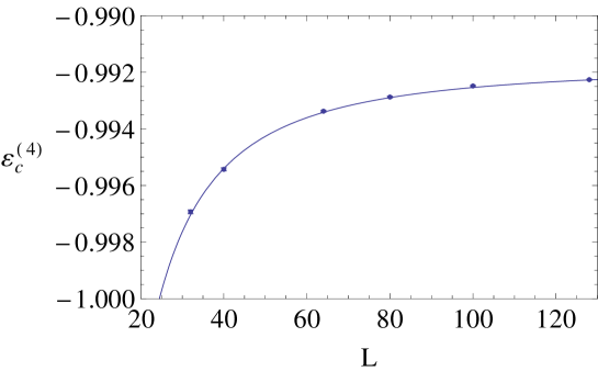
Figure 5: Energy density $\varepsilon^{(4)}_{c}$ at the critical temperature $T^{(4)}_{c}=1.06835$ as a function of $L$. The solid curve is the fit to Eq. (4) with $\alpha_{4}=-0.244$ and $\nu_{4}=0.7479$.

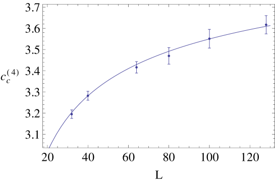
Figure 6: Specific heat $c^{(4)}_{c}$ at the critical temperature $T^{(4)}_{c}=1.06835$ as a function of $L$. The solid curve is the fit to (6) with $\alpha_{4}/\nu_{4}=-0.326$.

We fitted data of $c^{(4)}_{c}(L)$ reported in Table 11 according to the scaling relation given in Eq. (6) with $n=4$ and keeping the value of the ratio $\alpha_{4}/\nu_{4}$ fixed to $\alpha_{4}/\nu_{4}=-0.326$ as derived in Kanaya and Kaya (1995) at the same value of $T^{(4)}_{c}$ as in our case. The results of the fit are given by

$$\begin{split}c^{(4)}_{c}&=4.32\;\pm\;0.03\,,\\ c_{4}&=-3.46\;\pm\;0.10\,,\end{split}$$ (26)

and are reported in the first row of Table 13. To check the dependence of our results on the value of the ratio $\alpha_{4}/\nu_{4}$, we also performed the fit with a different choice for $\alpha_{4}/\nu_{4}$: $\alpha_{4}/\nu_{4}=-0.289$ as derived from data reported in Engels and Karsch (2012). The results of this fit are reported in the second row of Table 13. The values of $c^{(4)}_{c}$ reported in Table 13 are in a good agreement with each other. Moreover the value of $c^{(4)}_{c}$ in the second row Table 13 is consistent with the corresponding quantity reported in Engels and Karsch (2012) and derived with a rather different procedure.

Table 13: Fitting values of the parameters $c^{(4)}_{c}$ and $c_{4}$ entering expression (4) with $n=4$.

Fitting parameters	constants	results	$\chi^{2}/d.o.f$
		$c^{(4)}_{c}=4.32(3)$
$c^{(4)}_{c},\;c_{4}$	$\alpha_{4}/\nu_{4}=-0.326$	$c_{4}=-3.46(10)$	$0.12$
		$c^{(4)}_{c}=4.43(3)$
$c^{(4)}_{c},\;c_{4}$	$\alpha_{4}/\nu_{4}=-0.289$	$c_{4}=-3.37(9)$	$0.11$

In order to estimate $\varDelta\varepsilon^{(4),syst}_{c}$ we applied the two methods presented in Sec. III.1:

• Method 1. From Eq. (9), we computed the values of $\bar{\varepsilon}^{(4)}_{+}$ and $\bar{\varepsilon}^{(4)}_{-}$ at $T^{(4)}_{+}=1.06848$ and $T^{(4)}_{-}=1.06822$, respectively, assuming $\varepsilon^{(4)}_{c}=-0.99174$ as reported in Eq. (25). These quantities are given by $\bar{\varepsilon}^{(4)}_{+}=-0.991178$ and $\bar{\varepsilon}^{(4)}_{-}=-0.992302$ and are such that $|\varepsilon^{(4)}_{c}-\bar{\varepsilon}^{(4)}_{+}|=|\varepsilon^{(4)}_{c}-\bar{\varepsilon}^{(4)}_{-}|\simeq 0.0006$. In this way, we get

  $$\varDelta\bar{\varepsilon}^{(4),syst}_{c}=|\varepsilon^{(4)}_{c}-\bar{\varepsilon}^{(4)}_{\pm}|=0.0006.$$ (27)

• Method 2. We computed $\tilde{\varepsilon}^{(4)}_{\pm}$ with a fit of the energy density data $\tilde{\varepsilon}^{(4)}_{\pm}(L)$ with $L=32,64$ and $128$ derived with Monte Carlo simulations performed at $T^{(4)}_{+}=1.06848$ and $T^{(4)}_{-}=1.06822$, respectively; the fits have been computed according to relation in Eq. (12) with $n=4$ and $D_{4}=-0.326$ as in Kanaya and Kaya (1995). At variance with what we have done for $n=2$ and $3$, in this case we did not consider the values of the critical energy density for other $L$-values, obtained with Eq. (11). Indeed, in this case, the fits produced extremely bad results when Taylor-expanded data are considered. The Monte Carlo data involved in the analysis are given in Table 14; the statistical errors are reported in parentheses. The results of the fit, shown in Table 15, are such that

  $$\varDelta\tilde{\varepsilon}^{(4),syst}_{c}=\cdot^{|\varepsilon^{(4)}_{+}-\varepsilon^{(4)}_{c}|}_{|\varepsilon^{(4)}_{-}-\varepsilon^{(4)}_{c}|}=\cdot^{+0.00006}_{-0.00002}$$ (28)

As for the O$(2)$ and for the O$(3)$ model, we are going to consider $\varDelta\varepsilon^{(4),syst}_{c}=\varDelta\bar{\varepsilon}^{(4),syst}_{c}=0.0006$ given by Eq. (27), being larger than $\varDelta\tilde{\varepsilon}^{(4),syst}_{c}$ reported in Eq. (28).

We finally get

$$\varepsilon^{(4)}_{c}\;\pm\;\varDelta\varepsilon^{(4),stat}_{c}\;\pm\;\varDelta\varepsilon^{(4),syst}_{c}=-0.99174\;\pm\;0.00002\;\pm\;0.0006$$ (29)

as the final value of the critical energy density of the three dimensional O$(4)$ model in the thermodynamic limit. As for the O$(2)$ and the O$(3)$ models, the uncertainty on $\varepsilon^{(4)}_{c}$ due to $\varDelta T^{(4)}_{c}$ is larger than the statistical uncertainty.

Table 14: Energy density data $\varepsilon^{(4)}_{+}(L)$ and $\varepsilon^{(4)}_{-}(L)$ obtained with numerical Monte Carlo simulations performed at $T^{(4)}_{+}=1.06848$ and $T^{(4)}_{-}=1.06822$, respectively.

$L$	$\varepsilon^{(4)}_{+}(L)$	$\varepsilon^{(4)}_{-}(L)$
32	-0.996955(64)	-0.996962(67)
64	-0.993294(37)	-0.993383(36)
128	-0.992208(19)	-0.992275(18)

Table 15: Fitting values of the parameters $\varepsilon^{(4)}_{\pm}$ and $\varepsilon_{4,\pm}$.

Fitting parameters	$D_{4}$	results	$\chi^{2}/\text{d.o.f.}$
		$\varepsilon^{(4)}_{+}=-0.99168(3)$
$\varepsilon^{(4)}_{+},\;\varepsilon_{4,+}$	$D_{4}=-0.326$	$\varepsilon_{4,+}=-1.67(3)$	$1.5$
		$\varepsilon^{(4)}_{-}=-0.991755(8)$
$\varepsilon^{(4)}_{-},\;\varepsilon_{4,-}$	$D_{4}=-0.326$	$\varepsilon_{4,-}=-1.657(9))$	$0.16$

III.6 $n=\infty$, the spherical model

The spherical model has been introduced by Berlin and Kac Berlin and Kac (1952) as an exactly solvable model of a ferromagnet: its Hamiltonian reads

$$H^{sph}=-\sum_{\langle i,j\rangle}^{N}T_{i}T_{j}\,,$$ (30)

where the sum is intended over all the distinct pairs of distinct nearest neighbors on a regular $d-$dimensional hypercubic lattice. At variance with the O$(n)$ models, the “spin variables” $T_{i}$ are real numbers and their modulus is not fixed to unity: instead, the spherical constraint

$$\sum_{i=1}^{N}T^{2}_{i}=N$$ (31)

is imposed, allowing for a fluctuation of the modulus of the spin variables.

The spherical model is exactly solvable in any spatial dimension $d$ in the thermodynamic limit, both in the canonical and in the microcanonical ensembles: for the canonical solution see e.g. Binney et al. (1992) and references therein, for the microcanonical solution see Kastner (2009). Despite the long-range nature of the constraint in Eq. (31) the canonical and the microcanonical descriptions are equivalent and the model shows a continuous phase transition from a low-energy (temperature) ferromagnetic phase to a high-energy (temperature) paramagnetic phase for all $d\geq 3$ Joyce (1972a).

As pointed out in 1968 by H. E. Stanley, the free energy of a class of models described by the Hamiltonian

$${\mathbb{H}}^{(n)}=-\sum_{\langle i,j\rangle}^{N}\mathbf{T}^{(n)}_{i}\cdot\mathbf{T}^{(n)}_{j}=-\sum_{\langle i,j\rangle}^{N}\sum_{a=1}^{n}T^{a}_{i}T^{a}_{j}$$ (32)

(with $\mathbf{T}^{(n)}_{i}\equiv(T_{i}^{1},\ldots,T_{i}^{n})$ and $\,|\mathbf{T}_{i}|^{2}=n\;\forall i=1,\dots,N$) approaches the free energy of the spherical model (30) in the $n\rightarrow\infty$ limit Stanley (1968a). Moreover some “critical properties” of ${\mathbb{H}}^{(n)}$, like the value of the critical temperature $T^{(n)}_{c}$ or the value of some critical exponents Stanley (1968b), appear to be monotonic functions of $n$ .

The class of models described by the Hamiltonian in Eq. (32) can be mapped onto classical O$(n)$ models defined by Eq. (2), once the norm of the spins is properly scaled:

$${\mathbb{H}}^{(n)}=-\sum_{\langle i,j\rangle}^{N}\mathbf{T}^{(n)}_{i}\cdot\mathbf{T}^{(n)}_{j}=-n\sum_{\langle i,j\rangle}^{N}\mathbf{S}_{i}\cdot\mathbf{S}_{j}=n\;H^{(n)}\,,$$ (33)

so that

$$\lim_{n,\;N\rightarrow\infty}\frac{1}{n\;N}{\mathbb{H}}^{(n)}=\lim_{N\rightarrow\infty}\frac{1}{N}H^{(n)}=\lim_{N\rightarrow\infty}\frac{1}{N}H^{sph}.$$ (34)

This implies that the thermodynamic properties of the continuous O$(n)$ models described by the Hamiltonian in Eq. (2) converge to those of the spherical model in the $n\rightarrow\infty$ limit. In particular, the discrete set of critical values of the energy density: $\{\varepsilon^{(1)}_{c}$, $\varepsilon^{(2)}_{c}$, $\varepsilon^{(3)}_{c}$, $\varepsilon^{(4)}_{c},\dots\}$ should converge to $\varepsilon^{(\infty)}_{c}$ —that is to the critical energy density value of $H^{sph}$— in the $n\rightarrow\infty$ limit. This means that the spherical model has to be considered an O$(\infty)$ model in our analysis of the critical energy densities. The above property hold independently of the spatial dimensionality $d$ of the lattice, hence also in the case $d=3$.

In Binney et al. (1992); Kastner (2009) an explicit expression for $\varepsilon^{(\infty)}_{c}$ is given: when adapted to our conventions in $d=3$ the result is

$$\varepsilon^{(\infty)}_{c}=-3\;\;\frac{a_{3}}{1+a_{3}}\,,$$ (35)

where the coefficient $a_{3}$ is given by

$$a_{3}=\int_{[0,\pi]^{3}}\frac{d^{3}k}{\pi^{3}}\;\frac{\sum_{j=1}^{3}\cos{k_{j}}}{3-\sum_{j=1}^{3}\cos{k_{j}}}\,.$$ (36)

The coefficient $a_{3}$ is related to the Watson integral $W_{3}$ commonly used in the spherical model Joyce (1972a); Joyce and Zucker (2001): some properties of the Watson integrals are recalled in Appendix A. The result for $a_{3}$ is

$$a_{3}=\frac{\sqrt{3}-1}{32\pi^{3}}\left(\Gamma\left(\frac{1}{24}\right)\Gamma\left(\frac{11}{24}\right)\right)^{2}-1\,,$$ (37)

where $\Gamma$ denotes the gamma function. Using (37), the numerical value we get from Eq. (35) is

$$\varepsilon^{(\infty)}_{c}=-1.0216119\dots$$ (38)

and we shall use it as the critical energy density of the O$(\infty)$ model in $d=3$.

IV Comparison of critical energy densities

The critical energy densities $\varepsilon^{(n)}_{c}$, discussed in the previous Sections for $n=1,2,3,4$ and $\infty$, are collected in Table 16 as a function of $1/n=1/\infty,1/4,1/3,1/2$ and $1$, together with their derivation method.

Table 16: Critical energy densities $\varepsilon^{(n)}_{c}$ with their derivation method for $n=1,2,3,4$ and $n=\infty$.

$\frac{1}{n}$	$\varepsilon^{(n)}_{c}$	Derivation method
$\frac{1}{\infty}\equiv 0$	$-1.0216119\dots$	Exact solution
$\frac{1}{4}$	$-0.99174\;\pm\;0.00002\;\pm\;0.0006$	FSS this work, Eq.  (29)
$\frac{1}{3}$	$-0.989556\;\pm\;0.000010\;\pm\;0.00010$	FSS this work, Eq.  (24)
$\frac{1}{2}$	$-0.98904\;\pm\;0.00003\;\pm\;0.0003$	FSS this work, Eq.  (18)
1	$-0.99063\pm 0.00004$	FSS Hasenbusch and Pinn (1998)

Data in Table 16 can be interpolated to obtain an estimate of $\varepsilon^{(n)}_{c}$ for any $n$. To make such an interpolation more reliable, we exploit a theoretical result by Campostrini et al. Campostrini et al. (1996). These authors performed an analysis of the four-point renormalized coupling constant in classical O$(n)$ models. Interestingly, an important byproduct of their study was to have an estimate of the critical energy density $\varepsilon^{(n)}_{c}$ for large values of $n$, i.e., at the first order in a $1/n$ expansion. They found

$$\varepsilon^{(n)}_{c}=\varepsilon^{(\infty)}_{c}+b_{1}\,\frac{1}{n}+O\left(\frac{1}{n^{2}}\right)\,,$$ (39)

and the numerical result for the coefficient $b_{1}$ given in Campostrini et al. (1996), once adapted to our conventions, is $b_{1}=0.21$. The accuracy of $b_{1}$ affects the accuracy of the interpolation, as we shall see below, hence we repeated the numerical calculation of $b_{1}$ increasing its precision; as reported in Appendix A, we obtained $b_{1}=0.2182(8)$.

This result suggests an interpolation of the data in Table 16 has to be performed: $\varepsilon_{c}(n)$ should be a polynomial function in $\frac{1}{n}$ in which the zero-order term is given by the critical energy density $\varepsilon^{(\infty)}_{c}$ of the spherical model as given in Eq. (38), and the coefficient of the linear term is fixed to $b_{1}$. Using these constraints and the data of Table 16, we numerically computed the interpolating function and found

$$\varepsilon_{c}({n})=~{}\varepsilon^{(\infty)}_{c}+b_{1}\,\frac{1}{n}+b_{2}\,\frac{1}{n^{2}}+b_{3}\,\frac{1}{n^{3}}+b_{4}\,\frac{1}{n^{4}}$$ (40)

finding $b_{2}=-0.4762$, $b_{3}=0.3105$ and $b_{4}=0.0593$. In the interpolation procedure we did not consider the point $\{1,\varepsilon^{(1)}_{c}\}$ since our interest is in the comparison of $\varepsilon^{(n\geq 2)}_{c}$ and $\varepsilon^{(1)}_{c}$ in $\frac{1}{n}\in\left[0,\frac{1}{2}\right]$. Moreover, the function $\varepsilon_{c}(n)$ has to be computed with the lowest order polynomial function as possible. If we force $\varepsilon_{c}(n)$ to pass through $\{1,\varepsilon^{(1)}_{c}\}$, the next-order term ($b_{5}\,\frac{1}{n^{5}}$) becomes necessary although no useful information on $\varepsilon^{(n)}_{c}$ is present in the range $1/n\in[1/2,1]$. As a further check we also performed a fit of data presented in Table 16 (without the point $\{1,\varepsilon^{(1)}_{c}\}$) with a fourth-order polynomial obtaining an excellent agreement with the interpolation.

However, the value of $b_{1}$ is known with a finite precision, and this affects the reliability of the numerical values of the coefficients $b_{2}$, $b_{3}$ and $b_{4}$. To estimate the accuracy of the coefficients of the interpolation formula we thus repeated the procedure using $b_{1}=0.2190$ and $b_{1}=0.2174$, i.e., the upper and lower bounds for $b_{1}$, respectively. We can summarize the results as follows: the interpolation formula for the critical energy density is given by Eq. (40) with $\varepsilon^{(\infty)}_{c}=-1.0216119\dots$, $b_{1}=0.2182(8)$, $b_{2}=-0.472(7)$, $b_{3}=0.31(2)$ and $b_{4}=0.06(2)$.

In Fig. 7 we plot the following quantities: the interpolating curve given by Eq. (40) with the above reported coefficients (dashed blue line), the first-order approximation as given by Eq. (39) (solid green line), the horizontal curve $\varepsilon^{(n)}_{c}=\varepsilon^{(1)}_{c}$ in correspondence of the critical energy density of the Ising model (dot-dashed black line), and, with solid symbols, the critical energy densities $\varepsilon^{(1)}_{c}$, $\varepsilon^{(2)}_{c}$ (purple square), $\varepsilon^{(3)}_{c}$, $\varepsilon^{(4)}_{c}$ and $\varepsilon^{(\infty)}_{c}$ (blue down-pointing triangle). For $1/n=1/2,1/3,1/4$ the uncertainties on the points are given by the systematic uncertainties shown in Table 16 and are hardly visible on the plot being smaller than the symbols’ size. Simulation data for $n$ larger than 4 are not available. We thus reported on the plot the values of $\varepsilon^{(4)}_{c}$ obtained in Ref. Campostrini et al. (1996) with a strong-coupling expansion, using open symbols. Although these data are less accurate than simulation data they are in very good agreement with the interpolation formula.

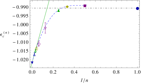
Figure 7: Critical energy densities $\varepsilon^{(n)}_{c}$ of 3-$d$ O$(n)$ models as a function of $1/n$: $\varepsilon^{(1)}_{c}$ (solid blue circle), $\varepsilon^{(2)}_{c}$ (solid purple square), $\varepsilon^{(3)}_{c}$ (solid yellow diamond), $\varepsilon^{(4)}_{c}$ (solid green up-pointing triangle) and $\varepsilon^{(\infty)}_{c}$ (solid blue down-pointing triangle) as given in Table 16; uncertainties are smaller than or of the same order of the symbol sizes. The dashed blue line is the interpolating curve $\varepsilon_{c}(1/n)$ given in Eq. (40) with the coefficients given in the text, the solid green line represents the $\frac{1}{n}$ expansion up to first order as given in Eq. (39), the horizontal dot-dashed black line is the line of equation $\varepsilon_{c}(n)=\varepsilon^{(1)}_{c}$. Open symbols are the values of the critical energies found by strong-coupling expansion in Ref. Campostrini et al. (1996) for $n=8$ (open purple down-pointing triangle), $n=16$ (open purple circle), $n=24$ (open yellow square), $n=32$ (open green diamond), and $n=48$ (open blue up-pointing triangle).

The interpolating curve provides a practical test for the reliability of the approximation $\varepsilon^{(n)}_{c}\simeq\varepsilon^{(1)}_{c}$ discussed at the beginning. Indeed, assuming that Eq. (40) yields good estimates of the values of $\varepsilon^{(n)}_{c}$, for any $n\in[2,\infty]$ the discrepancy between $\varepsilon^{(n)}_{c}$ and $\varepsilon^{(1)}_{c}$ can be easily quantified as $|\varepsilon_{c}(1/n)-\varepsilon^{(1)}_{c}|$. In particular: for $1/n\in[1,1/8)$, that is up to $n=8$, the error committed by replacing $\varepsilon^{(n)}_{c}$ with $\varepsilon^{(1)}_{c}$ is about $1\%$; for $1/n\in[1/8,1/18)$, that is up to $n=18$, the error is about $2\%$; for $1/n\in[1/18,0]$, that is up to $n=\infty$, the error is about $3\%$, and in any case smaller than $|\varepsilon^{(\infty)}_{c}-\varepsilon^{(1)}_{c}|\simeq 0.031$. We checked that the same conclusion is obtained by performing a fit of the form (40) using also the data for $\varepsilon^{(n)}_{c}$ with $n=8,16,24,32,48$ reported in Campostrini et al. (1996) (and of course the data of Table 16).

V Concluding remarks

We have performed a numerical analysis of the $n$-dependence of the critical energy density of three-dimensional classical O$(n)$ models defined on regular cubic lattices and with nearest-neighbor ferromagnetic interactions: our results are summarized in Table 16. For $n=2$ and $3$, our results for the critical energy densities —Eqs. (14) and (20)— improved the accuracy of the numerical estimates present in the literature.

The critical energy densities of classical O$(n)$ models with $n=2,3$ and $4$ have been evaluated with a finite-size scaling (FSS) analysis together with their statistical and systematic uncertainties due to the FSS procedure and to the uncertainty on the critical temperature, respectively; the systematic uncertainties turned out to be much larger (an order of magnitude) than the statistical ones for every value of $n$. A possible way to further reduce these systematic uncertainties in future simulations would possibly be to compute the critical temperature $T_{c}^{(n)}(L)$ at size $L$ Landau and Binder (2009), vary $L$ and then proceed to the FSS analysis.

Interpolating the data of $\varepsilon^{(n)}_{c}$ for $n=2,3,4$ and $n=\infty$, a polynomial function $\varepsilon_{c}(n)$ has been computed to estimate the critical energy density at any $n$. This function exploits the knowledge of the first-order term in the $1/n$-expansion of the critical energy density of O$(n)$ models computed in Campostrini et al. (1996), and yields a a practical way to test the error committed by replacing $\varepsilon^{(n)}_{c}$ with $\varepsilon^{(1)}_{c}$ for a generic O$(n)$ model. The latter is less than $1\%$ if $n\in[2,8)$, between $1\%$ and $2\%$ if $n\in[8,18]$ and less then $3\%$ for all the larger $n$’s up to $n=\infty$.

The above analysis concludes the discussion started in Casetti et al. (2011) as to the values of the critical energy densities of classical O$(n)$ models with ferromagnetic interactions defined on regular cubic lattices in $d=3$, showing that the critical energy densities of these models are indeed very close to each other and quantifying their differences. Clearly this result alone does not mean that the rather crude approximations on the density of states put forward in Casetti et al. (2011) are reliable. However, as already recalled in the Introduction, such approximations can be controlled and a relation similar to (1) can be derived for two exactly solvable models, the mean-field and 1-$d$ $XY$ models Nardini et al. (2012), and similar considerations can be effectively used to construct analytical or semi-analytical estimates of the density of states of O$(n)$ models that compare well with simulation data for $n=2$ in $d=2$ Nardini et al. (2013).

Finally a comment is in order on the critical energy densities for three-dimensional O$(n)$ models found in this paper. As briefly discussed in Sec. III.6, a monotonic behavior in $n$ is supposed to hold for some thermodynamic functions of classical O$(n)$ models defined on particular lattice geometries Stanley (1968b). It is unclear whether such considerations could be applied also to $\varepsilon^{(n)}_{c}$ of O$(n)$ models defined on regular cubic lattices. The interpolating function in Eq. (40) is a monotonically increasing function of $\frac{1}{n}$ from $n=\infty$ up to $n=2$, but this is no longer true for $n=1$ since —within the estimated errors— it is $\varepsilon^{(1)}_{c}<\varepsilon^{(2)}_{c}$. Monotonicity could be restored admitting a higher value $\varepsilon^{(1)\prime}_{c}$ for $\varepsilon^{(1)}_{c}$, such that $\varepsilon^{(1)\prime}_{c}-\varepsilon^{(1)}_{c}\simeq 10^{-3}$. The accuracy of the numerical value of $\varepsilon^{(1)}_{c}$ in Eq. (13) derived in Hasenbusch and Pinn (1998) clearly does not allow such a higher value of $\varepsilon^{(1)}_{c}$. Hence we conclude that monotonicity fails for $n=1$, unless the uncertainty quoted in Hasenbusch and Pinn (1998) is underestimated. However, a possible increase of $10^{-3}$ in $\varepsilon^{(1)}_{c}$ would neither affect the considerations made at the end of Sec. IV nor the form of Eq. (40).

Appendix A Some properties of the Watson integrals and estimate of $b_{1}$

The Watson integrals appear in the theory of the spherical model Joyce (1972a) and are related to the generalized Watson integrals

$$W(d,z)=\frac{1}{\pi^{d}}\,\int_{0}^{\pi}\cdots\int_{0}^{\pi}\,\frac{dk_{1}\cdots dk_{d}}{1-\frac{1}{dz}\left(\cos{k_{1}}+\cdots+\cos{k_{d}}\right)}\,.$$ (41)

The Watson integral in dimension $d$ is defined as

$$W_{d}=\frac{1}{\pi^{d}}\,\int_{0}^{\pi}\cdots\int_{0}^{\pi}\,\frac{dk_{1}\cdots dk_{d}}{d-\left(\cos{k_{1}}+\cdots+\cos{k_{d}}\right)}\,,$$ (42)

so that

$$d\,W_{d}=W(d,1)\,.$$ (43)

Using the notation

$$f_{d}(\mathbf{k})\equiv d-\sum_{\alpha=1}^{d}\cos{k_{\alpha}}\,$$ (44)

with $\mathbf{k}=(k_{1},\ldots,k_{d})$, the Watson integral $W_{d}$ can be compactly written in the form

$$W_{d}=\int_{[0,\pi]^{d}}\,\frac{d^{d}k}{\pi^{d}}\,\frac{1}{f_{d}(\mathbf{k})}\,.$$ (45)

The coefficient $a_{d}$ defined in Eq. (36) for $d=3$ reads in dimension $d$

$$a_{d}=\int_{[0,\pi]^{d}}\,\frac{d^{d}k}{\pi^{d}}\,\frac{\sum_{\alpha=1}^{d}\cos{k_{\alpha}}}{f_{d}(\mathbf{k})}\,:$$ (46)

$a_{d}$ is related to the Watson integral $W_{d}$ according to the relation

$$a_{d}=d\,W_{d}-1\,.$$ (47)

A major simplification in the evaluation of Watson integrals is obtained by using the identity Maradudin et al. (1960)

$$\frac{1}{\lambda}=\int_{0}^{\infty}\,e^{-\lambda t}\,dt\,:$$ (48)

by putting $\lambda=f_{d}(\mathbf{k})=d-\sum_{\alpha=1}^{d}\cos{k_{\alpha}}$ in Eq. (42) and integrating over the $k_{\alpha}$’s one gets the single integral

$$W_{d}=\int_{0}^{\infty}\,e^{-dt}\,[I_{0}(t)]^{d}\,dt\,,$$ (49)

where $I_{0}(t)=(1/\pi)\,\int_{0}^{\pi}e^{t\cos{k}}\,dk$ is a modified Bessel function of the first kind.

In $d=3$ it is possible to write $W_{d}$ in terms of the gamma function Watson (1939); Joyce (1972b); Borwein and Zucker (1992) as

$$W_{3}=\frac{\sqrt{3}-1}{96\pi^{3}}\left(\Gamma\left(\frac{1}{24}\right)\Gamma\left(\frac{11}{24}\right)\right)^{2}\,,$$ (50)

from which Eq. (37) follows.

The Watson integral in $d=3$ and its generalizations enter as well in the coefficients of the $1/n$ expansion Campostrini et al. (1996); Müller and Rühl (1986): in particular the coefficient $b_{1}$ defined in the expression (39) for the critical energy density reads as Campostrini et al. (1996)

$$b_{1}=2\left(\frac{b_{1}^{(a)}}{4}-\frac{1}{W_{3}}-\frac{b_{1}^{(b)}}{\left(W_{3}\right)^{2}}\right)\,,$$ (51)

where the coefficients $b_{1}^{(a)},b_{1}^{(b)}$ are computed as integrals of the function $\Delta(\mathbf{q})$ defined as

$$\frac{1}{\Delta(\mathbf{q})}=\frac{1}{8}\int_{[-\pi,\pi]^{3}}\frac{d^{3}k}{(2\pi)^{3}}\,\frac{1}{f_{3}\left(\mathbf{k}\right)\,f_{3}\left(\mathbf{k+q}\right)}\,,$$ (52)

with $\mathbf{q}$ belonging to the first Brillouin zone ($\mathbf{q}\in[\pi,\pi]^{3}$) and $f_{3}\left(\mathbf{k}\right)=3-\sum_{\alpha=x,y,z}\cos{k_{\alpha}}$. We observe that using twice the identity (48) one can formally reduce the integral in (52) to a double integral as

$$\frac{1}{\Delta(\mathbf{q})}=\frac{1}{8}\int_{0}^{\infty}dt_{1}\,e^{-3t_{1}}\int_{0}^{\infty}dt_{2}\,e^{-3t_{2}}\,\left(\prod_{\alpha=x,y,z}{\cal I}\left(q_{\alpha};t_{1},t_{2}\right)\right)\,$$ (53)

[similarly to the re-writing (49) for $W_{d}$] with

$${\cal I}\left(q;t_{1},t_{2}\right)=\int_{-\pi}^{\pi}\,\frac{dk}{2\pi}\,e^{\,t_{1}\,\cos{k}+t_{2}\,\cos{(k+q)}}\,.$$ (54)

The expressions for $b_{1}^{(a)}$ and $b_{1}^{(b)}$ are respectively given by

$$b_{1}^{(a)}=\frac{1}{2}\,\int_{[-\pi,\pi]^{3}}\frac{d^{3}q}{(2\pi)^{3}}\,\frac{\Delta(\mathbf{q})}{f_{3}\left(\mathbf{q}\right)}\,$$ (55)

and

$$b_{1}^{(b)}=-\frac{1}{16}\,\int_{[-\pi,\pi]^{3}}\frac{d^{3}q}{(2\pi)^{3}}\,\Delta(\mathbf{q})\int_{[-\pi,\pi]^{3}}\frac{d^{3}p}{(2\pi)^{3}}\frac{1}{\left(f_{3}\left(\mathbf{p}\right)\right)^{2}}\left[\frac{1}{f_{3}\left(\mathbf{p+q}\right)}+\frac{1}{f_{3}\left(\mathbf{p-q}\right)}-\frac{2}{f_{3}\left(\mathbf{q}\right)}\right]\,.$$ (56)

Numerically we obtained $b_{1}^{(a)}=6.49628(1)$ and $b_{1}^{(b)}=-0.1184(1)$, from which $b_{1}=0.2182(8)$.

References

- Casetti et al. (2011) L. Casetti, C. Nardini, and R. Nerattini, Phys. Rev. Lett. 106, 057208 (2011).
- Nardini et al. (2012) C. Nardini, R. Nerattini, and L. Casetti, Journal of Statistical Mechanics: Theory and Experiment 2012, P02007 (2012).
- Nardini et al. (2013) C. Nardini, R. Nerattini, and L. Casetti, (2013), arXiv:1312.5223 .
- Wales (2004) D. J. Wales, Energy Landscapes (Cambridge University Press, Cambridge, 2004).
- Note (1) The relation (1\@@italiccorr) cannot be exact, at least in the form proposed in Casetti et al. (2011), because it would imply wrong —and -independent— values of the critical exponent . Nevertheless Eq. (1) yields the correct sign of , that is, correctly predicts a cusp in the specific heat at criticality and not a divergence: see Refs. Casetti et al. (2011) and especially Nardini et al. (2012) for a more complete discussion on the problem.
- Campa et al. (2003) A. Campa, A. Giansanti, and D. Moroni, Journal of Physics A: Mathematical and General 36, 6897 (2003).
- Archambault et al. (1997) P. Archambault, S. T. Bramwell, and P. C. W. Holdsworth, Journal of Physics A: Mathematical and General 30, 8363 (1997).
- de Souza and Brady Moreira (1993) A. J. F. de Souza and F. G. Brady Moreira, Phys. Rev. B 48, 9586 (1993).
- Gottlob and Hasenbusch (1993) A. P. Gottlob and M. Hasenbusch, Physica A: Statistical Mechanics and its Applications 201, 593 (1993).
- Brown and Ciftan (2006) R. G. Brown and M. Ciftan, Phys. Rev. B 74, 224413 (2006).
- Engels and Karsch (2012) J. Engels and F. Karsch, Phys. Rev. D 85, 094506 (2012).
- Stanley (1968a) H. E. Stanley, Phys. Rev. 176, 718 (1968a).
- Campostrini et al. (1996) M. Campostrini, A. Pelissetto, P. Rossi, and E. Vicari, Nuclear Physics B 459, 207 (1996).
- Hasenbusch and Pinn (1998) M. Hasenbusch and K. Pinn, Journal of Physics A: Mathematical and General 31, 6157 (1998).
- Note (2) But in the case , that will be discussed in Sec. III.6.
- (16) Web page: http://alps.comp-phys.org/ .
- Fisher (1974) M. E. Fisher, Rev. Mod. Phys. 46, 597 (1974).
- Brèzin (1982) E. Brèzin, J. Physique 43, 15 (1982).
- Stanley (1999) H. E. Stanley, Rev. Mod. Phys. 71, S358 (1999).
- Schultka and Manousakis (1995) N. Schultka and E. Manousakis, Phys. Rev. B 52, 7528 (1995).
- Note (3) For only the statistical error will be computed since this quantity is only used for the computation of .
- Note (4) Notice that Eqs. (4) and Eq. (12) hold for - however, since for the models considered, we assume Eq. (12) valid in the whole range .
- Talapov and Blöte (1996) A. L. Talapov and H. W. J. Blöte, Journal of Physics A: Mathematical and General 29, 5727 (1996).
- Landau and Binder (2009) D. P. Landau and K. Binder, A Guide to Monte Carlo Simulations in Statistical Physics, 3rd ed. (Cambridge University Press, Cambridge, 2009).
- Goldner and Ahlers (1992) L. S. Goldner and G. Ahlers, Phys. Rev. B 45, 13129 (1992).
- Hasenbusch and Török (1999) M. Hasenbusch and T. Török, Journal of Physics A: Mathematical and General 32, 6361 (1999).
- Le Guillou and Zinn-Justin (1980) J. C. Le Guillou and J. Zinn-Justin, Phys. Rev. B 21, 3976 (1980).
- Holm and Janke (1994) C. Holm and W. Janke, Journal of Physics A: Mathematical and General 27, 2553 (1994).
- Kanaya and Kaya (1995) K. Kanaya and S. Kaya, Phys. Rev. D 51, 2404 (1995).
- Berlin and Kac (1952) T. H. Berlin and M. Kac, Phys. Rev. 86, 821 (1952).
- Binney et al. (1992) J. J. Binney, N. J. Dowrick, A. J. Fisher, and M. Newman, The Theory of Critical Phenomena: An Introduction to the Renormalization Group (Oxford University Press, New York, 1992).
- Kastner (2009) M. Kastner, Journal of Statistical Mechanics: Theory and Experiment 2009, P12007 (2009).
- Joyce (1972a) G. S. Joyce, in Phase Transitions and Critical Phenomena, Vol. 2, edited by C. Domb and M. S. Green (Academic Press, 1972).
- Stanley (1968b) H. E. Stanley, Phys. Rev. Lett. 20, 589 (1968b).
- Note (5) In Stanley (1968b) the monotonicity is explicitly shown for the above quantities in and for particular geometries of the lattices, i.e., spin chains, triangular lattices and fcc lattices. These results are supposed to hold also in more general cases but the generalization is not straightforward. In particular, it is not immediately clear whether the monotonicity is expected to hold also also for the energy density of models defined by Eq. (2) on regular cubic lattices in .
- Joyce and Zucker (2001) G. S. Joyce and I. J. Zucker, Journal of Physics A: Mathematical and General 34, 7349 (2001).
- Maradudin et al. (1960) A. A. Maradudin, E. W. Montroll, G. H. Weiss, R. Herman, and H. W. Milnes, Green’s Functions for Monoatomic Simple Cubic Lattice (Académie Royale de Belgique, Bruxelles, 1960).
- Watson (1939) G. N. Watson, Q. J. Math. Oxford 10, 266 (1939).
- Joyce (1972b) G. S. Joyce, Journal of Physics A: Mathematical and General 5, L65 (1972b).
- Borwein and Zucker (1992) J. M. Borwein and I. J. Zucker, IMA J. Numer. Anal. 12, 519 (1992).
- Müller and Rühl (1986) V. F. Müller and W. Rühl, Annals of Physics 168, 425 (1986).