CPMC-Lab: A Matlab Package for
Constrained Path Monte Carlo Calculations

Abstract

We describe CPMC-Lab, a Matlab program for the constrained-path and phaseless auxiliary-field Monte Carlo methods. These methods have allowed applications ranging from the study of strongly correlated models, such as the Hubbard model, to ab initio calculations in molecules and solids. The present package implements the full ground-state constrained-path Monte Carlo (CPMC) method in Matlab with a graphical interface, using the Hubbard model as an example. The package can perform calculations in finite supercells in any dimensions, under periodic or twist boundary conditions. Importance sampling and all other algorithmic details of a total energy calculation are included and illustrated. This open-source tool allows users to experiment with various model and run parameters and visualize the results. It provides a direct and interactive environment to learn the method and study the code with minimal overhead for setup. Furthermore, the package can be easily generalized for auxiliary-field quantum Monte Carlo (AFQMC) calculations in many other models for correlated electron systems, and can serve as a template for developing a production code for AFQMC total energy calculations in real materials. Several illustrative studies are carried out in one- and two-dimensional lattices on total energy, kinetic energy, potential energy, and charge- and spin-gaps.

Keywords: Quantum Monte Carlo, Auxiliary Field Quantum Monte Carlo, Constrained Path Monte Carlo, sign problem, Hubbard model, pedagogical software

PROGRAM SUMMARY

Manuscript Title: CPMC-Lab: A Matlab Package for Constrained Path Monte Carlo Calculations
Authors: Huy Nguyen, Hao Shi, Jie Xu and Shiwei Zhang
Program Title: CPMC-Lab
Journal Reference:
Catalogue identifier:
Licensing provisions: CPC non-profit license
Programming language: Matlab
Computer: The non-interactive scripts can be executed on any computer capable of running Matlab with all Matlab versions. The GUI requires Matlab R2010b (version 7.11) and above.
Operating system: Windows, Mac OS X, Linux
RAM: variable.
Number of processors used: 1
Keywords: Quantum Monte Carlo, Auxiliary Field Quantum Monte Carlo (AFQMC), Constrained Path Monte Carlo (CPMC), sign problem, Hubbard model, pedagogical software
Classification: 7.3 Electronic Structure
External routines/libraries: Matlab
Nature of problem: Obtaining ground state energy of a repulsive Hubbard model in a supercell in any number of dimensions
Solution method: In the Constrained Path Monte Carlo (CPMC) method, the ground state of a many-fermion system is projected from an initial trial wave function by a branching random walk in an overcomplete basis of Slater determinants. Constraining the determinants according to a trial wave function $\ket{\Psi_{\mathrm{T}}}$ removes the exponential decay of the signal-to-noise ratio characteristic of the sign problem. The method is exact if $\ket{\Psi_{\mathrm{T}}}$ is exact.
Unusual features: Direct and interactive environment with a Graphical User Interface for beginners to learn and study the Constrained Path Monte Carlo method with minimal overhead for setup.

References

[1] S. Zhang, J. Carlson and J. E. Gubernatis, Phys. Rev. B. 55, 7464 (1997).

[2] Shiwei Zhang, in the free online book “Emergent Phenomena in Correlated Matter Modeling and Simulation, vol 3,” eds. E. Pavarini, E. Koch, and U. Schollwock (2013). http://www.cond-mat.de/events/correl13

I Introduction

The study of interacting quantum many-body systems remains an outstanding challenge, especially systems with strong particle interactions, where perturbative approaches are often ineffective. Numerical simulations provide a promising approach for studying such systems. One of the most general numerical approaches is quantum Monte Carlo (QMC) methods based on auxiliary fields, which are applied in condensed matter physics, nuclear physics, high-energy physics and quantum chemistry. These methods allow essentially exact calculations of ground-state and finite-temperature equilibrium properties of interacting many fermion systems.

As is well-known, however, these methods suffer from the sign problem which severely limits their applicability. Considerable progress has been achieved in circumventing this problem by constraining the random walks while sampling the space of auxiliary fields Zhang (2013). Many applications of this method involve lattices where there is a sign problem, for example, Hubbard-like models where the local interactions lead to auxiliary-fields that are real. In these cases the method is known as Constrained Path Monte Carlo (CPMC) Zhang et al. (1997); Chang and Zhang (2008). The method can also be generalized to treat realistic electron-electron interactions to allow for ab initio calculations on real materials Zhang and Krakauer (2003); Al-Saidi et al. (2006). For these systems there is a phase problem because the Coulomb interaction leads to complex auxiliary fields. In such systems, the method is referred to as phaseless or phase-free auxiliary-field QMC (AFQMC). In both cases (lattice and continuum), the idea behind the method is to constrain the sign or phase of the overlap of the sampled Slater determinants with a trial wave function. The constraint eliminates the sign or phase instability and restores low power (typically to the third power of system size) computational scaling. Applications to systems ranging from lattice models Chang and Zhang (2010); Shi and Zhang (2013) of correlated systems to solids Purwanto et al. (2009a); Ma et al. (2013) to atoms and molecules Purwanto et al. (2011) have shown that these methods are very accurate, even with simple trial wave functions taken directly from Hartree-Fock or density-functional calculations.

Since these methods combine standard mean-field approaches with stochastic QMC, they pose a formidable barrier to beginners. As such, it is useful to have a pedagogical platform to learn the methods and to aid further code development. In this paper, we present a Matlab package that fulfills these roles. The package illustrates the CPMC method for the Hubbard model, with a graphical interface. The ground-state energy is calculated using importance sampling and implementing the full algorithmic details. With this open-source package, calculations can be performed directly on Hubbard-like models in any dimensions, under any boundary conditions. It will be straightforward to generalize the code for applications in many other models of correlated electron systems. Furthermore, the code contains the core QMC algorithmic ingredients for a total energy AFQMC calculation. These ingredients can be combined with standard electronic structure machineries Martin (2004) (see, e.g., Refs Gonze et al. (2009) and Valiev et al. (2010)) to develop a production code for AFQMC total energy calculations in molecules and solids.

The tool presented here allows users to experiment with various model and run parameters and visualize the results. For this purpose Matlab offers many advantages over traditional programing languages such as FORTRAN or C. As an interpreted language, Matlab requires no compilation, is platform-independent and allows easy interaction with the algorithm during runtime. Matlab also provides an array of tools to visualize results from computations including a full graphical user interface (GUI). These advantages make the package a better choice for our purposes, as discussed above, than regular “production” codes, despite a large discrepancy in computational speed. We provide several examples and include more questions in the exercises, which illustrate the usage of the code, key algorithmic features, how to compute various properties in the Hubbard model, and how to generalize it for other applications. As a pedagogical tool, the package can be used in combination with the lecture notes in Ref. Zhang (2013) and references therein.

The remainder of the paper is organized as follows. In Section II we introduce the formalism and various technical ingredients of the CPMC method, and notations used in the rest of this paper. In Section III the actual algorithm is outlined in detail. An overview of the software package and instructions is given in Section IV, including a list of exercises. In Section V, we briefly discuss the computational cost and comment on the relation between this package and one written in a more conventional numerical programming language. Then in Section VI, we present several applications which illustrate algorithmic issues; benchmark the method; discuss CPMC calculations of the kinetic energy, potential energy and double occupancy; and report several new CPMC results on the spin- and charge-gaps. We summarize in Section VII and include a list of some useful Matlab commands in A.

II Method and Notation

The ground-state CPMC algorithm has two main components: The first component is the formulation of the ground state projection as an open-ended importance-sampled random walk. This random walk takes place in Slater determinant space rather than configuration space like in Green’s function Monte Carlo (GFMC) Kalos et al. (1974); Ceperley and Kalos (1979). There are two ways to perform this random walk. Traditional projector QMC uses an exact unconstrained projection that suffers from exponential scaling in computational cost with increasing system size due to the sign problem. In contrast, CPMC achieves polynomial scaling by using an approximate constrained projection, which becomes exact if the trial wave function (used to impose the constraint) is identical to the ground state. Furthermore, importance sampling makes CPMC a more efficient way to do projector QMC in many cases. The second component is the constraint of the paths of the random walk so that any Slater determinant generated during the random walk maintains an appropriate overlap with a known trial wave function $\ket{\psi_{\mathrm{T}}}$. This constraint eliminates the sign decay, making the CPMC method scale algebraically instead of exponentially, but introduces a systematic error in the algorithm. These two components are independent of each other, and can be used separately. We call the combination of these two components the ground-state CPMC algorithm. This section only briefly reviews the application of CPMC to the Hubbard model. The reader is referred to Refs. Zhang et al. (1997); Zhang (2013) and references therein for a discussion of the Hubbard model implementation and generalization of this theory to other, more realistic Hamiltonians.

II.1 Slater determinant space

The CPMC method works with a chosen one-particle basis. A Born-Oppenheimer Hamiltonian with standard electronic interactions does not mix the spins. We assume in the discussion below that the Hamiltonian conserves total $\hat{S}_{z}$, and that the number of electrons with each spin component is fixed. It is straightforward to treat a Hamiltonian that does mix the spin species Shi et al. (2014).

We will use the following notation:

• $M$: the number of single-electron basis states i.e. the number of lattice sites in the Hubbard model.

• $\ket{\chi_{i}}$: the $i$-th single-particle basis state ($i=1,2,\dots,M$).

• $c^{\dagger}_{i}$ and $c_{i}$: creation and annihilation operators for an electron in $\ket{\chi_{i}}$. $n_{i}\equiv c^{\dagger}_{i}c_{i}$ is the corresponding number operator.

• $N$: the number of electrons. $N_{\sigma}$ is the number of electrons with spin $\sigma$ ($\sigma=\uparrow$ or $\downarrow$). As expected, $N_{\sigma}\leq M$.

• $\varphi$: a single-particle orbital. The coefficients in the expansion $\varphi=\sum_{i}\varphi_{i}\ket{\chi_{i}}=\sum_{i}c^{\dagger}_{i}\varphi_{i}\ket{0}$ in the single particle basis $\{\ket{\chi_{i}}\}$ can be conveniently expressed as an $M$-dimensional vector:

  $$\begin{pmatrix}\varphi_{1}\\ \varphi_{2}\\ \vdots\\ \varphi_{M}\end{pmatrix}$$ (1)

• $\ket{\phi}$: a many-body wave function which can be written as a Slater determinant. Given $N$ different single-particle orbitals, we form a many-body wave function from their anti-symmetrized product:

  $$\ket{\phi}\equiv\hat{\varphi}_{1}^{\dagger}\hat{\varphi}_{2}^{\dagger}\cdots\hat{\varphi}_{N}^{\dagger}\ket{0}$$ (2)

  where the operator $\hat{\varphi}_{m}^{\dagger}\equiv\sum_{i}c_{i}^{\dagger}\,\varphi_{i,m}$ creates an electron in the $m$-th single-particle orbital as described in Eq. (1).

• $\Phi$: an $M\times N$ matrix which represents the coefficients of the orbitals used to construct a Slater determinant $\ket{\phi}$:

  $$\Phi\equiv\begin{pmatrix}\varphi_{1,1}&\varphi_{1,2}&\cdots&\varphi_{1,N}\\ \varphi_{2,1}&\varphi_{2,2}&\cdots&\varphi_{2,N}\\ \vdots&\vdots&&\vdots\\ \varphi_{M,1}&\varphi_{M,2}&\cdots&\varphi_{M,N}\end{pmatrix}$$ (3)

  Each column of this matrix is an $M$-dimensional vector and represents a single-particle orbital described by Eq. (1). For brevity, we will subsequently refer to this $M\times N$ matrix as a Slater determinant.

• $\ket{\Psi}$ (upper case): a many-body wave function which is not necessarily a single Slater determinant, e.g. the many-body ground state $\ket{\Psi_{0}}$.

We list several properties of a Slater determinant. First, for any two non-orthogonal Slater determinants, $\ket{\phi}$ and $\ket{\phi^{\prime}}$, it can be shown that their overlap integral is given by a number:

$$\braket{\phi}{\phi^{\prime}}=\det\left(\Phi^{\mathrm{\dagger}}\Phi^{\prime}\right),$$ (4)

where $\Phi^{\mathrm{\dagger}}$ is the conjugate transpose of the matrix $\Phi$.

Second, the operation on any Slater determinant in Eq. (2) by the exponential of a one body operator

$$\hat{B}=\exp\left(\sum_{ij}^{M}c_{i}^{\dagger}U_{ij}c_{j}\right)$$ (5)

simply leads to another Slater determinant Hamann and Fahy (1990):

$$\hat{B}\ket{\phi}=\hat{\phi}_{1}^{\prime\,\dagger}\hat{\phi}_{2}^{\prime\,\dagger}\cdots\hat{\phi}_{N}^{\prime\;\dagger}\,\ket{0}\equiv\ket{\phi^{\prime}}$$ (6)

with $\hat{\phi}_{m}^{\prime\;\dagger}=\sum_{j}c_{j}^{\dagger}\,\Phi^{\prime}_{jm}$ and $\Phi^{\prime}\equiv\mathrm{e}^{U}\Phi$, where the matrix $U$ is formed from elements $U_{ij}$. Since $B\equiv\mathrm{e}^{U}$ is an $M\times M$ square matrix, the operation of $\hat{B}$ on $\ket{\phi}$ simply involves multiplying $\mathrm{e}^{U}$, an $M\times M$ matrix, to $\Phi$, an $M\times N$ matrix.

As mentioned above, operations on the spin-up sector do not affect the spin-down sector and vice versa. Thus it is convenient to represent each Slater determinant as two independent spin parts:

$$\ket{\phi}=\ket{\phi^{\uparrow}}\otimes\ket{\phi^{\downarrow}}$$ (7)

The corresponding matrix representation is

$$\Phi=\Phi^{\uparrow}\otimes\Phi^{\downarrow}$$ (8)

where $\Phi^{\uparrow}$ and $\Phi^{\downarrow}$ have dimensions $M\times N_{\uparrow}$ and $M\times N_{\downarrow}$, respectively. The overlap between any two Slater determinants is simply the product of the overlaps of individual spin determinants:

$$\braket{\phi}{\phi^{\prime}}=\prod_{\sigma=\uparrow,\downarrow}\braket{\phi^{\sigma}}{\phi^{\prime\sigma}}=\det\left[(\Phi^{\uparrow})^{\mathrm{\dagger}}\Phi^{\prime\uparrow}\right]\cdot\det\left[(\Phi^{\downarrow})^{\mathrm{\dagger}}\Phi^{\prime\downarrow}\right]\,.$$ (9)

Any operator $\hat{B}$ described by Eq. (5) acts independently on the two spin parts:

$$\hat{B}\ket{\phi}=\hat{B}^{\uparrow}\ket{\phi^{\uparrow}}\otimes\hat{B}^{\downarrow}\ket{\phi^{\downarrow}}$$ (10)

Each of the spin components of $\hat{B}$ can be represented as an $M\times M$ matrix. Applying $\hat{B}$ to a Slater determinant simply involves matrix multiplications for the $\uparrow$ and $\downarrow$ components separately, leading to another Slater determinant $\ket{\phi^{\prime}}$ as in Eq. (6) i.e. the result is $B^{\uparrow}\Phi^{\uparrow}\otimes B^{\downarrow}\Phi^{\downarrow}$. Unless specified, the spin components of $\hat{B}$ are identical i.e. $B^{\uparrow}=B^{\downarrow}$ (note the absence of a hat on $B$ to denote the matrix of the operator $\hat{B}$).

II.2 The Hubbard Hamiltonian

The one-band Hubbard model is a simple paradigm of a system of interacting electrons. Its Hamiltonian is given by

$$\hat{H}=\hat{K}+\hat{V}=-t\sum_{\langle ij\rangle\sigma}(c_{i\sigma}^{\dagger}c_{j\sigma}^{\phantom{\dagger}}+c_{j\sigma}^{\dagger}c_{i\sigma}^{\phantom{\dagger}})+U\sum_{i}n_{i\uparrow}n_{i\downarrow},$$ (11)

where $t$ is the hopping matrix element, and $c_{i\sigma}^{\dagger}$ and $c_{i\sigma}$ are electron creation and destruction operators, respectively, of spin $\sigma$ on site $i$. The Hamiltonian is defined on a lattice of dimension $M=\prod_{d}L_{d}$. The lattice sites serve as the basis functions here, i.e., $\ket{\chi_{i}}$ denotes an electron localized on the site labeled by $i$. The notation $\langle\;\rangle$ in Eq. (11) indicates nearest-neighbors. The on-site Coulomb repulsion is $U>0$, and the model only has two parameters: the strength of the interaction $U/t$ and the electron density $(N_{\uparrow}+N_{\downarrow})/M$. In this paper we will use $t$ as the unit of energy and set $t=1$.

The difference between the Hubbard Hamiltonian and a general electronic Hamiltonian is in the structure of the matrix elements in $\hat{K}$ and $\hat{V}$. In the latter, $\hat{K}$ is specified by hopping integrals of the form $K_{ij}$, while $\hat{V}$ is specified by Coulomb matrix elements of the form $V_{ijkl}$, with $i,j,k,l$ in general running from $1$ to $M$. In terms of the CPMC method, the structure of $\hat{K}$ makes essentially no difference. The structure of $\hat{V}$, however, dictates the form of the Hubbard-Stratonovich transformation (see Section II.3.1) . For the Hubbard interaction, the resulting one-body propagators turn out to be real, as shown below, while for the general case complex propagators arise and cause a phase problem Zhang (2013).

II.3 Ground-state projection

We will focus on ground-state calculations in this paper. (Finite-temperature generalizations to the grand-canonical ensemble also exist Zhang (1999); Rubenstein et al. (2012).) The ground-state wave function $\ket{\Psi_{0}}$ can be obtained from any trial wave function $\ket{\Psi_{\mathrm{T}}}$ that is not orthogonal to $\ket{\Psi_{0}}$ by repeated applications of the ground-state projection operator

$$\mathcal{P}_{\mathrm{gs}}=\mathrm{e}^{-\Delta\tau(\hat{H}-E_{\mathrm{T}})}$$ (12)

where $E_{\mathrm{T}}$ is the best guess of the ground-state energy. That is, if the wave function at the $n$-th time step is $\ket{\Psi^{(n)}}$, the wave function at the next time step is given by

$$\ket{\Psi^{(n+1)}}=\mathrm{e}^{-\Delta\tau(\hat{H}-E_{\mathrm{T}})}\ket{\Psi^{(n)}}$$ (13)

With a small $\Delta\tau$, the second-order Trotter approximation can be used:

$$\mathrm{e}^{-\Delta\tau\hat{H}}=\mathrm{e}^{-\Delta\tau(\hat{K}+\hat{V})}\approx\mathrm{e}^{-\Delta\tau\,\hat{K}/2}\mathrm{e}^{-\Delta\tau\,\hat{V}}\mathrm{e}^{-\Delta\tau\,\hat{K}/2}\,.$$ (14)

The residual Trotter error can be removed by, for example, extrapolation with several independent runs of sufficiently small $\Delta\tau$ values. We illustrate this technique in an exercise in Section IV.2.2.

II.3.1 The Hubbard-Stratonovich transformation

In Eq. (14), the kinetic energy (or, more generally, one-body) propagator $\hat{B}_{\mathrm{K/2}}\equiv\mathrm{e}^{-\Delta\tau\hat{K}/2}$ has the same form as Eq. (5). However, the potential energy propagator $\mathrm{e}^{-\Delta\tau\hat{V}}$ does not. A Hubbard-Stratonovich (HS) transformation can be employed to transform $\mathrm{e}^{-\Delta\tau\hat{V}}$ into the desired form. In the Hubbard model, we can use the following:

$$e^{-\Delta\tau Un_{i\uparrow}n_{i\downarrow}}=\mathrm{e}^{-\Delta\tau U(n_{i\uparrow}+n_{i\downarrow})/2}\sum_{x_{i}=\pm 1}p(x_{i})\,\mathrm{e}^{\gamma x_{i}(n_{i\uparrow}-n_{i\downarrow})}\,,$$ (15)

where $\gamma$ is given by $\cosh(\gamma)=\exp(\Delta\tau U/2)$. We interpret $p(x_{i})=1/2$ as a discrete probability density function (PDF) with $x_{i}=\pm 1$.

In Eq. (15), the exponent on the left, which comes from the interaction term $\hat{V}$ on the $i$-th site, is quadratic in $n$, indicating the interaction of two electrons. The exponents on the right, on the other hand, are linear in $n$, indicating two non-interacting electrons in a common external field characterized by $x_{i}$. Thus an interacting system has been converted into a non-interacting system living in fluctuating external auxiliary fields $x_{i}$, and the summation over all such auxiliary-field configurations recovers the many-body interactions. The special form of HS for the Hubbard interaction is due to Hirsch Hirsch (1985). The linearized operator on the right hand side in Eq. (15) is the spin $(n_{i\uparrow}-n_{i\downarrow})$ on each site.

In this paper and in the code, we will use the discrete spin decomposition in Eq. (15). There exist other ways to do the HS transformation, e.g. based on the Gaussian integral:

$$\mathrm{e}^{\hat{A}^{2}}=\frac{1}{\sqrt{2\pi}}\int_{-\infty}^{\infty}\mathrm{d}x\,\mathrm{e}^{-x^{2}/2}\;\mathrm{e}^{\sqrt{2}x\,\hat{A}}\,.$$ (16)

There is also a charge version of the discrete HS transformation involving the linearized operator $n_{i\uparrow}+n_{i\downarrow}$, the total charge on each site.

Different forms of the HS transformation can have different efficiencies in different situations. In particular, preserving the appropriate symmetries of the system can significantly reduce the statistical fluctuations and reduce the error from the constrained-path approximation Shi and Zhang (2013).

Since we represent a Slater determinant as individual spin determinants in Eq. (7), it is convenient to spin-factorize Eq. (15) as

$$\mathrm{e}^{-\Delta\tau Un_{i\uparrow}n_{i\downarrow}}=\sum_{x_{i}=\pm 1}p(x_{i})\left[\hat{b}^{\uparrow}_{V}(x_{i})\otimes\hat{b}^{\downarrow}_{V}(x_{i})\right]$$ (17)

where the spin-dependent operator $\hat{b}^{\sigma}_{V}(x_{i})$ on the $i$-th lattice site is defined as

$$\hat{b}^{\sigma}_{\mathrm{V}}(x_{i})=\mathrm{e}^{-[\Delta\tau U/2-s(\sigma)\,\gamma\,x_{i}]c_{i\sigma}^{\dagger}c_{i\sigma}}$$ (18)

and $s(\uparrow)=+1$ and $s(\downarrow)=-1$. The related operator $\hat{b}_{\mathrm{V}}(x_{i})$ (i.e. without $\sigma$) includes both the spin up and spin down parts. Below we will use the corresponding symbol without hat ($b_{\mathrm{V}}$) to denote the matrix representation of the operator ($\hat{b}_{\mathrm{V}}$) associated with that symbol.

The potential energy propagator $\mathrm{e}^{-\Delta\tau\hat{V}}$ over all sites can easily be seen to be the product of the propagators $\mathrm{e}^{-\Delta\tau Un_{i\uparrow}n_{i\downarrow}}$ over each site:

$$\mathrm{e}^{-\Delta\tau\hat{V}}=\sum_{\vv{x}}P(\vv{x})\prod_{\sigma=\uparrow,\downarrow}\hat{B}^{\sigma}_{V}(\vv{x})$$ (19)

where $\vv{x}=\{x_{1},\dots,x_{M}\}$ is one configuration of auxiliary fields over all $M$ sites and $\hat{B}^{\sigma}_{V}(\vv{x})=\prod_{i}\hat{b}^{\sigma}_{V}(x_{i})$ is the $\vv{x}$-dependent product of the spin-$\sigma$ propagators over all sites. The overall PDF here is $P(\vv{x})=\prod_{i}p(x_{i})=\left(\frac{1}{2}\right)^{M}$, to be distinguished from the PDF $p$ for one individual auxiliary field $x_{i}$ in Eq. (17).

Now the projection operator in Eq. (12) can be expressed entirely in terms of operators in Eq. (5)

$$\mathcal{P}_{\mathrm{gs}}\approx\mathrm{e}^{\Delta\tau E_{\mathrm{T}}}\sum_{\vv{x}}P(\vv{x})\prod_{\sigma=\uparrow,\downarrow}\hat{B}^{\sigma}_{\mathrm{K/2}}\hat{B}^{\sigma}_{\mathrm{V}}(\vv{x})\hat{B}^{\sigma}_{\mathrm{K/2}}$$ (20)

As noted in Eq. (10), $B_{\mathrm{K/2}}$ has an $\uparrow$ and a $\downarrow$ component, each of which is an $M\times M$ matrix. Applying each $\hat{B}_{\mathrm{K/2}}$ to a Slater determinant $\ket{\phi}$ simply involves matrix multiplications with the matrix $B_{\mathrm{K/2}}$ for the $\uparrow$ and $\downarrow$ components of $\Phi$ separately, leading to another Slater determinant $\ket{\phi^{\prime}}$ as in Eq. (6).

II.3.2 A toy model for illustration

Let us take, for example, a simple one-dimensional four-site Hubbard model with $N_{\uparrow}=2$, $N_{\downarrow}=1$ and open boundary condition. The sites are numbered sequentially.

First let us examine the trivial case of free electrons i.e. $U=0$. We can write down the one-electron Hamiltonian matrix, which is of dimension $4\times 4$:

$$H=\begin{pmatrix}0&-1&0&0\\ -1&0&-1&0\\ 0&-1&0&-1\\ 0&0&-1&0\end{pmatrix}$$ (21)

Direct diagonalization gives us the eigenstates of $H$ from which we immediately obtain the matrix $\Phi_{0}$ for the ground-state wave function $\ket{\psi_{0}}$:

$$\Phi_{0}=\begin{pmatrix}0.3717&-0.6015\\ 0.6015&-0.3717\\ 0.6015&\phantom{-}0.3717\\ 0.3717&\phantom{-}0.6015\end{pmatrix}\otimes\begin{pmatrix}0.3717\\ 0.6015\\ 0.6015\\ 0.3717\end{pmatrix}$$ (22)

where the first matrix contains two single-particle orbitals (two columns) for the two $\uparrow$ electrons and the second matrix contains one single-electron orbital for the one $\downarrow$ electron. Each single-electron orbital is an eigenvector of $H$.

The matrix $\Phi_{0}$ represents $\ket{\phi_{0}}$ in the same way that Eq. (3) represents Eq. (2). Of course, the solution above is also the restricted Hartree-Fock solution to the interacting problem. We will often use $\Phi_{0}$ as the trial wave function in CPMC below.

Next we consider the interacting problem, with $U>0$. Applying the HS transformation of Eq. (15) to Eq. (14), we have

$$\mathcal{P}_{\mathrm{gs}}=\mathrm{e}^{\Delta\tau E_{\mathrm{T}}-\Delta\tau U(N_{\uparrow}+N_{\downarrow})/2}\sum_{\vec{x}}P(\vec{x})\;B_{\mathrm{K/2}}\cdot\begin{pmatrix}\mathrm{e}^{\gamma x_{1}}&0&0&0\\ 0&\mathrm{e}^{\gamma x_{2}}&0&0\\ 0&0&\mathrm{e}^{\gamma x_{3}}&0\\ 0&0&0&\mathrm{e}^{\gamma x_{4}}\end{pmatrix}\cdot B_{\mathrm{K/2}}\\ \otimes B_{\mathrm{K/2}}\cdot\begin{pmatrix}\mathrm{e}^{-\gamma x_{1}}&0&0&0\\ 0&\mathrm{e}^{-\gamma x_{2}}&0&0\\ 0&0&\mathrm{e}^{-\gamma x_{3}}&0\\ 0&0&0&\mathrm{e}^{-\gamma x_{4}}\end{pmatrix}\cdot B_{\mathrm{K/2}}\,,$$ (23)

where $\vec{x}=\{x_{1},x_{2},x_{3},x_{4}\}$ and $P(\vv{x})=\left(\frac{1}{2}\right)^{4}$. This is just Eq. (20) specialized to a four-site lattice.

II.4 Random walk in Slater determinant space

The first component of the CPMC algorithm is the reformulation of the projection process as branching, open-ended random walks in Slater determinant space (instead of updating a fixed-length path in auxiliary-field space).

Let us define $B_{\mathrm{V}}(\vv{x})=\prod_{\sigma}B^{\sigma}_{V}(\vv{x})$ as we have done for $\hat{b}_{\mathrm{V}}$. Applying the HS-transformed propagator in Eq. (20) to one projection step in Eq. (13) gives

$$\ket{\phi^{(n+1)}}=\mathrm{e}^{\Delta\tau E_{\mathrm{T}}}\sum_{\vv{x}}P(\vv{x})\left[\hat{B}_{\mathrm{K/2}}\hat{B}_{\mathrm{V}}(\vv{x})\hat{B}_{\mathrm{K/2}}\right]\ket{\phi^{(n)}}\,.$$ (24)

In the Monte Carlo (MC) realization of this iteration, we represent the wave function at each stage by a finite ensemble of Slater determinants, i.e.

$$\ket{\Psi^{(n)}}\propto\sum_{k}\ket{\phi^{(n)}_{k}}$$ (25)

where $k$ labels the Slater determinants and an overall normalization factor of the wave function has been omitted. These Slater determinants will be referred to as random walkers.

The iteration in Eq. (24) is achieved stochastically by MC sampling of $\vv{x}$. That is, for each random walker $\ket{\phi^{(n)}_{k}}$, we choose an auxiliary-field configuration $\vv{x}$ according to the PDF $P(\vv{x})$ and propagate the determinant to a new determinant via $\ket{\phi^{(n+1)}_{k}}=\hat{B}_{\mathrm{K/2}}\hat{B}_{\mathrm{V}}(\vv{x})\hat{B}_{\mathrm{K/2}}\ket{\phi^{(n)}_{k}}$.

We repeat this procedure for all walkers in the population. These operations accomplish one step of the random walk. The new population represents $\ket{\Psi^{(n+1)}}$ in the sense of Eq. (25), i.e. $\ket{\Psi^{(n+1)}}\propto\sum_{k}\ket{\phi_{k}^{(n+1)}}$. These steps are iterated until sufficient data has been collected. After an equilibration phase, all walkers thereon are MC samples of the ground-state wave function $\ket{\Psi_{0}}$ and ground-state properties can be computed. We will refer to this type of approach as free projection. In practice, branching occurs because of the re-orthonormalization of the walkers, which we discuss below in Section II.8. We emphasize that the statistical error bar can be reduced significantly with more “optimal” forms of HS transformations to extend the reach of free-projection calculations (see e.g., Refs. Zhang (2013); Shi and Zhang (2013)).

II.5 Importance sampling

To improve the efficiency of Eq. (24) and make it a practical and scalable algorithm, an importance sampling scheme Zhang (2013); Kalos et al. (1974); Ceperley and Kalos (1979) is required. In the procedure just described above, no information is contained in the sampling of $\vv{x}$ on the importance of the resulting determinant in representing $\ket{\Psi_{0}}$. Computing the mixed estimator of the ground-state energy

$$E_{\mathrm{mixed}}\equiv\frac{\braket{\phi_{\mathrm{T}}}{\hat{H}}{\Psi_{0}}}{\braket{\phi_{\mathrm{T}}}{\Psi_{0}}}$$ (26)

requires estimating the denominator by $\sum_{k}\braket{\phi_{\mathrm{T}}}{\phi_{k}}$ where $\ket{\phi_{k}}$ are random walkers after equilibration. Since these walkers are sampled with no knowledge of $\braket{\phi_{\mathrm{T}}}{\phi_{k}}$, terms in the summation over $\ket{\phi_{k}}$ can have large fluctuations that lead to large statistical errors in the MC estimate of the denominator, thereby in that of $E_{\mathrm{mixed}}$.

With importance sampling, first we define an importance function:

$$O_{\mathrm{T}}(\phi_{k})\equiv\braket{\phi_{\mathrm{T}}}{\phi_{k}}\,,$$ (27)

which estimates the overlap of a Slater determinant $\ket{\phi}$ with the ground-state wave function (approximated here by a trial wave function). As in Diffusion Monte Carlo (DMC) Umrigar et al. (1993), we also assign a weight $w_{k}=O_{\mathrm{T}}(\phi_{k})$ to each walker. This weight is initialized to unity for all walkers since in the initial ensemble, $\ket{\phi_{k}^{(0)}}=\ket{\phi_{\mathrm{T}}}$ for all $k$.

We then iterate a formally different but mathematically equivalent version of Eq. (24):

$$\ket{\widetilde{\phi}^{(n+1)}}\leftarrow\sum_{\vv{x}}\widetilde{P}(\vv{x})\hat{B}(\vv{x})\ket{\widetilde{\phi}^{(n)}}$$ (28)

where

$$\hat{B}(\vv{x})=\hat{B}_{\mathrm{K/2}}\hat{B}_{\mathrm{V}}(\vv{x})\hat{B}_{\mathrm{K/2}}\,.$$ (29)

The walkers $\ket{\widetilde{\phi}^{(n)}}$ are now sampled from a new distribution. They schematically represent the ground-state wave function by:

$$\ket{\Psi^{(n)}}\propto\sum_{k}w^{(n)}\frac{\ket{\phi^{(n)}_{k}}}{O_{\mathrm{T}}(\phi^{(n)}_{k})}\,,$$ (30)

in comparison to Eq. (25).

The modified function $\widetilde{P}(\vv{x})$ in Eq. (28) is $\widetilde{P}(\vv{x})=\prod_{i}^{M}\widetilde{p}(x_{i})$, where the probability for sampling the auxiliary-field at each lattice site is given by

$$\widetilde{p}(x_{i})=\frac{O_{\mathrm{T}}(\phi^{(n)}_{k,i})}{O_{\mathrm{T}}(\phi^{(n)}_{k,i-1})}\,p(x_{i}).$$ (31)

where

$$\ket{\phi^{(n)}_{k,i-1}}=\hat{b}_{V}(x_{i-1})\,\hat{b}_{V}(x_{i-2})\,\cdots\,\hat{b}_{V}(x_{1})\,\ket{\phi^{(n)}_{k}}$$ (32)

is the current state of the $k$-th walker, ${\ket{\phi^{(n)}_{k}}}$, after its first $(i-1)$ fields have been sampled and updated, and

$$\ket{\phi^{(n)}_{k,i}}=\hat{b}_{V}(x_{i})\ket{\phi^{(n)}_{k,i-1}}$$ (33)

is the next sub-step after the $i$-th field is selected and the walker is updated. Note that in the notation above $\ket{\phi^{(n)}_{k,0}}=\ket{\phi^{(n)}_{k}}$ and $\ket{\phi^{(n)}_{k,M}}=\ket{\phi^{(n+1)}_{k}}$. As expected, $\widetilde{P}(\vv{x})$ is a function of both the current and future positions in Slater-determinant space. Further, $\widetilde{P}(\vv{x})$ modifies $P(\vv{x})$ such that the probability of sampling $\vv{x}$ is increased when $\vv{x}$ leads to a determinant with larger overlap with $\ket{\phi_{\mathrm{T}}}$ and is decreased otherwise. In each $\widetilde{p}(x_{i})$, $x_{i}$ can only take the value of $+1$ or $-1$ and can be sampled by a heatbath-like algorithm: choosing $x_{i}$ from the PDF $\widetilde{p}(x_{i})/N_{i}$ where the normalization factor is

$$\mathcal{N}_{i}\equiv\widetilde{p}(x_{i}=+1)+\widetilde{p}(x_{i}=-1)\,,$$ (34)

and carrying a weight for the walker

$$w^{(n)}_{k,i}=\mathcal{N}_{i}w^{(n)}_{k,i-1}\,,$$ (35)

in which we have used the same notation as in Eqs. (32) and (33). The ratio of the overlaps in Eq. (31), involving a change of only one site (or even a few sites if desired), can be computed quickly using the Sherman-Morrison formula, as shown in the code. The inverse of the overlap matrix $\left[(\Phi_{\mathrm{T}})^{\dagger}\Phi_{k}^{(n)}\right]^{-1}$ is kept and updated after each $x_{i}$ is selected.

It should be pointed out that a significant reduction in computational cost is possible in the present code. Because the free-electron trial wave function is used here, the overlap matrix can be trivially updated after each application of $\hat{B}_{\mathrm{K/2}}$. In the code, however, the update is still carried out explicitly in order to allow for a more general form of the trial wave function.

We note that, for a general continuous auxiliary-field, the importance sampling can be achieved by a force bias Zhang and Krakauer (2003); Purwanto and Zhang (2004); Zhang (2013). The above discrete version can be viewed as a two-point realization of the continuous case.

II.6 The sign problem and the constrained path approximation

II.6.1 The sign problem

The sign problem occurs because of the fundamental symmetry between the fermion ground state $\ket{\Psi_{0}}$ and its negative $-\ket{\Psi_{0}}$ Zhang and Kalos (1991). This symmetry implies that, for any ensemble of Slater determinants $\{\ket{\phi}\}$ which gives a Monte Carlo representation of the ground-state wave function, there exists another ensemble $\{-\ket{\phi}\}$ which is also a correct representation. In other words, the Slater determinant space can be divided into two degenerate halves ($+$ and $-$) whose bounding surface $\mathcal{N}$ is defined by $\braket{\Psi_{0}}{\phi}=0$. This surface is in general unknown. Except for some special cases Hirsch (1985), walkers do cross $\mathcal{N}$ in their propagation by $\mathcal{P}_{\mathrm{gs}}$, causing the sign problem. At the instant such a walker lands on $\mathcal{N}$, the walker will make no further contribution to the representation of the ground state at any later time because

$$\braket{\Psi_{0}}{\phi}=0\ \implies\braket{\Psi_{0}}{\mathrm{e}^{-\tau H}}{\phi}=0\quad\text{for any }\tau$$ (36)

Paths that result from such a walker have equal probabilities of being in either half of the Slater determinant space Zhang (2013). Computed analytically, they would cancel and make no contribution in the ground-state wave function. However, because the random walk has no knowledge of $\mathcal{N}$, these paths continue to be sampled (randomly) in the random walk and become Monte Carlo noise.

To eliminate the decay of the signal-to-noise ratio, we impose the constrained path approximation. It requires that each random walker at each step have a positive overlap with the trial wave function $\ket{\phi_{\mathrm{T}}}$:

$$\braket{\phi_{\mathrm{T}}}{\phi_{k}^{(n)}}>0.$$ (37)

This yields an approximate solution to the ground-state wave function, $\ket{\Psi^{\mathrm{c}}_{0}}=\sum_{\phi}\ket{\phi}$, in which all Slater determinants $\ket{\phi}$ satisfy Eq. (37). Note that from Eq. (36), the constrained path approximation becomes exact for an exact trial wave function $\ket{\psi_{\mathrm{T}}}=\ket{\Psi_{0}}$. The constrained path approximation is easily implemented by redefining the importance function in Eq. (27):

$$O_{\mathrm{T}}(\phi_{k})\equiv\operatorname{max}\{\braket{\phi_{\mathrm{T}}}{\phi_{k}},0\}$$ (38)

This prevents walkers from crossing the trial nodal surface ${\cal N}$ and entering the “$-$” half-space as defined by $\ket{\phi_{\mathrm{T}}}$. We note that imposing Eq. (37) is fundamentally different from just discarding the negative contributions in the denominator of Eq. (26); the constrained path condition results in a distribution of walkers that vanishes smoothly at the interface between the “$+$” and “$-$” parts of the determinant space. The use of a finite $\Delta\tau$ causes a small discontinuity which is a form of Trotter error in the constraint; this error can be further reduced Zhang (2000).

II.6.2 Twist boundary condition and the phase problem

Our simulations are carried out in supercells of finite sizes. For most quantities that we wish to calculate, the periodic boundary condition (PBC) causes large finite-size effects, often compounded by significant shell effects Chang and Zhang (2008). In order to reduce these effects and reach the thermodynamic limit more rapidly, it is more effective to use the twist boundary condition (TBC) and average over the twist angles Lin et al. (2001); Chang and Zhang (2008) (TABC). Under the TBC, the wave function $\Psi(\mathbf{r_{1}},\mathbf{r_{2}},\dots,\mathbf{r_{N}})$ gains a phase when electrons hop around lattice boundaries:

$$\Psi(\dots,\mathbf{r_{j}+L},\dots)=\mathrm{e}^{\mathrm{i}\,\mathbf{\widehat{L}}\cdot\bm{\Theta}}\Psi(\dots,\mathbf{r_{j}},\dots)\,,$$ (39)

where $\mathbf{\widehat{L}}$ is the unit vector along $\mathbf{L}$ and the twist angle $\bm{\Theta}=(\theta_{x},\theta_{y},\theta_{z},\dots)$ is a parameter with $\theta_{d}\in(-\pi,\pi]$ for $d=x,y,z,\dots$. It is implemented straightforwardly as a modification to the matrix elements in the $\hat{K}$ part of the Hamiltonian. A twist is equivalent to shifting the underlying momentum space grid by $(\theta_{x}/L_{x},\theta_{y}/L_{y},\theta_{z}/L_{z},\cdots)$. Symmetry can be used to reduce the range of $\bm{\Theta}$. One could either choose to have a special grid of $\bm{\Theta}$ values Martin (2004) or choose them randomly Lin et al. (2001); Chang and Zhang (2008). In the illustrations we will use the latter. The QMC results are averaged, and the MC error bar will be the combined statistical errors from the random $\bm{\Theta}$ distribution and from each QMC calculation for a particular $\bm{\Theta}$.

With a general twist angle, the AFQMC method will have a “phase problem” instead of the sign problem described above. This is because the hopping matrix elements in $\hat{K}$ now have complex numbers which make the orbitals in the random walkers complex. The stochastic nature of the random walk will then lead to an asymptotic distribution which is symmetric in the complex plane Zhang and Krakauer (2003); Zhang (2013). For each walker $\ket{\phi}$, instead of a $+\ket{\phi}$ and $-\ket{\phi}$ as in the sign problem, there is now an infinite set $\{\mathrm{e}^{\mathrm{i}\theta}\ket{\phi}\}$ ($\theta\in[0,2\pi]$) from which the random walk cannot distinguish.

The phase problem that occurs in the present case is a “milder” form of the most general phase problem, because here the phases arise from the one-body hopping term instead of the two-body interaction term. The latter takes place in a long-range Coulomb interaction, for example. In that case, the phase problem is controlled with the phaseless or phase-free approximation Zhang and Krakauer (2003); Zhang (2013). When the phase only enters as a one-body boundary condition, the stochastic auxiliary-fields are not directly coupled to complex numbers. A simple generalization of the constrained-path approximation suffices Chang and Zhang (2008): at each step of propagation, the random walkers are required to satisfy the constraint

$$\operatorname{Re}\left\{\frac{\braket{\phi_{\mathrm{T}}}{\phi_{k}^{(n+1)}}}{\braket{\phi_{\mathrm{T}}}{\phi_{k}^{(n)}}}\right\}>0$$ (40)

where $\ket{\phi^{(n)}_{k}}$ and $\ket{\phi^{(n+1)}_{k}}$ are the current and proposed walkers. Note that Eq. (38) is a special case of Eq. (40) because $\braket{\phi_{\mathrm{T}}}{\phi_{k}^{(0)}}>0$ and all overlaps are real when $\hat{K}$ is real. We emphasize that, when the HS transformation leads to complex one-body propagators as in the case of realistic electronic problems, an extra step is required to “importance-transform” the propagators using the phase of the overlap Zhang and Krakauer (2003); Zhang (2013).

II.6.3 Systematic error from the constrained-path approximation, and its reduction and removal

Most applications have used a single-determinant $\ket{\psi_{\mathrm{T}}}$ taken directly from a Hartree-Fock (HF) or density-functional theory (DFT) calculations. In the Hubbard model, the restricted HF wave function is the same as the free-electron wave function, while the unrestricted HF wave function breaks spin-symmetry and allows, for example, antiferromagnetism and spin-density-wave states Xu et al. (2011). A large number of benchmarks have been carried out with these wave functions Shi and Zhang (2013); Zhang (2013).

Figure 1 illustrates the effectiveness of the constrained path approximation. The system is a $4\times 4$ lattice with 7 spin-$\uparrow$ and 7 spin-$\downarrow$ electrons, $U=4$ and $\bm{\Theta}=(0.02\pi,0.04\pi)$. The free-projection (FP) run exhibits growing statistical fluctuations as a function of projection time, indicative of the sign problem. With the constraint, CPMC fluctuations are always smaller with the same amount of computational cost, and they are independent of projection time. The CPMC results converge to a value below the exact result (horizontal line).

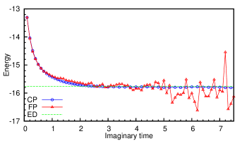
Figure 1: (Color online) Illustration of the sign problem. The blue and red curves show the energy during a projection from $\tau=0$ to $\tau=7.5$ with and without the constraint, respectively. The dashed black line shows the exact result. The CP error bars are too small to be seen. To improve clarity, only every other CP energy measurements are shown for $\tau>2.6$.

Multi-determinant trial wave functions can reduce the systematic error because they are better variational wave functions Purwanto et al. (2009b). Using wave functions that restore symmetries of the system can reduce the systematic error significantly Shi and Zhang (2013). The symmetry restoration can be either in the form of a multi-determinant trial wave function or from symmetry projection Shi et al. (2014). For example, using a 10-determinant symmetry trial wave function can reduce the systematic error in the CPMC result for the system in Fig. 1 with periodic boundary condition by a significant factor Shi and Zhang (2013).

Recently, it has been demonstrated Purwanto et al. (2009a); Shi and Zhang (2013); Sorella (2011) that free-projection and release-constraint calculations allow systematic removal of the constrained-path bias by “lifting” the constraint (and bringing back the sign problem). This offers another avenue for systematically improvable AFQMC calculations.

II.7 Energy measurement

CPMC-Lab uses the mixed estimator in Eq. (26) for the ground-state energy which, for an ensemble $\{\ket{\phi}\}$, is given by:

$$E_{\mathrm{mixed}}=\frac{\sum_{k}w_{k}\,E_{\mathrm{L}}\left[\phi_{\mathrm{T}},\phi_{k}\right]}{\sum_{k}w_{k}}$$ (41)

where the local energy $E_{\mathrm{L}}$ is:

$$E_{\mathrm{L}}\left[\phi_{\mathrm{T}},\phi\right]=\frac{\braket{\phi_{\mathrm{T}}}{\hat{H}}{\phi}}{\braket{\phi_{\mathrm{T}}}{\phi}}$$ (42)

This quantity can be easily evaluated for any walker $\phi$ as follows. For any pair of Slater determinants $\ket{\phi_{\mathrm{T}}}$ and $\ket{\phi}$, we can calculate the one-body equal-time Green’s function as:

$$\braket{c_{j\sigma}^{\dagger}c_{i\sigma}}\equiv\frac{\braket{\phi_{\mathrm{T}}}{c_{j\sigma}^{\dagger}c_{i\sigma}}{\phi}}{\braket{\phi_{\mathrm{T}}}{\phi}}=\left[\Phi^{\sigma}\,[\,(\Phi_{\mathrm{T}}^{\sigma})^{\dagger}\Phi^{\sigma}\,]^{-1}(\Phi_{\mathrm{T}}^{\sigma})^{\dagger}\right]_{ij}\,.$$ (43)

This immediately enables the computation of the kinetic energy term $\Braket{\phi_{\mathrm{T}}}{-t\sum_{\braket{ij}\sigma}c_{i\sigma}^{\dagger}c_{j\sigma}}{\phi}$. The potential energy term $\Braket{\phi_{\mathrm{T}}}{U\sum_{i}c_{i\uparrow}^{\dagger}c_{i\uparrow}^{\phantom{\dagger}}c_{i\downarrow}^{\dagger}c_{i\downarrow}^{\phantom{\dagger}}}{\phi}$ does not have the form of Eq. (43), but can be reduced to that form by an application of Wick’s theorem:

$$\braket{c_{i\uparrow}^{\dagger}c_{i\uparrow}^{\phantom{\dagger}}c_{i\downarrow}^{\dagger}c_{i\downarrow}^{\phantom{\dagger}}} =\braket{c_{i\uparrow}^{\dagger}c_{i\uparrow}}\braket{c_{i\downarrow}^{\dagger}c_{i\downarrow}}+\braket{c_{i\uparrow}^{\dagger}c_{i\downarrow}}\braket{c_{i\uparrow}c_{i\downarrow}^{\dagger}}$$

$$=\braket{c_{i\uparrow}^{\dagger}c_{i\uparrow}}\braket{c_{i\downarrow}^{\dagger}c_{i\downarrow}}$$ (44)

The reduction to the last line occurs because the $\uparrow$ and $\downarrow$ spin sectors are decoupled in both $\ket{\phi_{\mathrm{T}}}$ and $\ket{\phi}$. (This is not the case in a pairing Carlson et al. (2011) or generalized Hartree-Fock wave function Shi et al. (2014). The former is the desired form for $U<0$. The latter can be used to improve the quality of the trial wave function for $U>0$, and is necessary if the Hamiltonian contains spin-orbit coupling.)

The mixed estimator for the energy arises naturally from importance sampling, and reduces the statistical variance of the computed result. A drawback of the mixed estimator is that the ground-state energy obtained in AFQMC under the constrained path approximation is not variational Zhang (2013). The mixed estimators for observables which do not commute with the Hamiltonian are biased. The back-propagation technique can be used to obtain pure estimates Zhang et al. (1997); Purwanto and Zhang (2004).

II.8 Other implementation issues

II.8.1 Population control

As the random walk proceeds, some walkers may accumulate very large weights while some will have very small weights. These different weights cause a loss of sampling efficiency because the algorithm will spend a disproportionate amount of time keeping track of walkers that contribute little to the energy estimate. To eliminate the inefficiency of carrying these weights, a branching scheme is introduced to “redistribute” the weights without changing the statistical distribution. In such a scheme, walkers with large weights are replicated and walkers with small weights are eliminated with some probability.

However, because branching might cause the population to fluctuate in an unbounded way (e.g. to grow to infinity or to perish altogether), we perform population control to eliminate this instability at the cost of incurring a bias when the total weight of the walkers is modified. This bias can be reduced by carrying a history of overall weight correction factors. However, the longer this history is included in the energy estimators, the higher the statistical noise. In this package we use a simple “combing” method Calandra Buonaura and Sorella (1998), which discards all history of overall weight normalizations. We note that there exist more elaborate approaches Umrigar et al. (1993); Zhang et al. (1997); Calandra Buonaura and Sorella (1998), for example, keeping a short history of the overall weight renormalization. The length of the history to keep should be a compromise between reducing bias (long) and keeping statistical fluctuation from becoming much larger (short). The effect of population control and how to extrapolate away the bias are illustrated in the Exercises.

II.8.2 Re-orthonormalization

Repeated multiplications of $B_{\mathrm{K/2}}$ and $B_{\mathrm{V}}$ to a Slater determinant in Eq. (24) lead to numerical instability, such that round-off errors dominate and $\ket{\phi^{(n)}_{k}}$ represents an unfaithful propagation of $\ket{\phi^{(0)}_{k}}$. This instability is controlled by periodically applying the modified Gram-Schmidt orthonormalization to each Slater determinant. For each walker $\ket{\phi}$, we factor its corresponding matrix as $\Phi=QR$ where $R$ is a upper triangular matrix and $Q$ is a matrix whose columns are orthonormal vectors representing the re-orthonormalized single-particle orbitals. After this factorization, $\Phi$ is replaced by $Q$ and the corresponding overlap $O_{\mathrm{T}}$ by $O_{\mathrm{T}}/\det(R)$ because $Q$ contains all the information about the walker $\ket{\phi}$ while $R$ only contributes to the overlap of $\ket{\phi}$. With importance sampling, only the information in $Q$ is relevant and $R$ can be discarded.

III Algorithm

1. For each walker, specify its initial state. Here we use the trial wave function $\Phi_{\mathrm{T}}$ as the initial state and assign the weight $w$ and overlap $O_{\mathrm{T}}$ each a value of unity.

2. If the weight of a walker is nonzero, propagate it via $B_{\mathrm{K/2}}$ as follows:

   1. Perform the matrix-matrix multiplication

      $$\Phi^{\prime}=B_{\mathrm{K/2}}\Phi$$ (45)

      (recall the convention that $B_{\mathrm{K/2}}$ denotes the matrix of $\hat{B}_{\mathrm{K/2}}$) and compute the new importance function

      $$O_{\mathrm{T}}^{\prime}=O_{\mathrm{T}}(\phi^{\prime})\,.$$ (46)

      (We can also work in momentum space, e.g., by using fast Fourier transforms.)

   2. If $O_{\mathrm{T}}^{\prime}\neq 0$, update the walker, weight and $O_{\mathrm{T}}$ as

      $$\Phi\leftarrow\Phi^{\prime}\,,\quad w\leftarrow w\,O_{\mathrm{T}}^{\prime}/O_{\mathrm{T}}\,,\quad O_{\mathrm{T}}\leftarrow O_{\mathrm{T}}^{\prime}$$ (47)

3. If the walker’s weight is still nonzero, propagate it via $B_{\mathrm{V}}(\vv{x})$ as follows

   1. Compute the inverse of the overlap matrix

      $$O_{\mathrm{inv}}=\left(\Phi_{\mathrm{T}}^{\dagger}\Phi\right)^{-1}$$ (48)

   2. For each auxiliary field $x_{i}$, do the following:

      1. Compute $\widetilde{p}(x_{i})$

      2. Sample $x_{i}$ and update the weight as

         $$w\leftarrow w[\widetilde{p}(x_{i}=+1)+\widetilde{p}(x_{i}=-1)]$$ (49)

      3. If the weight of the walker is still not zero, propagate the walker by performing the matrix multiplication

         $$\Phi^{\prime}=b_{\mathrm{V}}(x_{i})\,\Phi$$ (50)

         and then update $O_{\mathrm{T}}$ and $O_{\mathrm{inv}}$.

4. Repeat step 2.

5. Multiply the walker’s weight by a normalization factor:

   $$w\leftarrow w\,\mathrm{e}^{\Delta\tau E_{\mathrm{T}}}$$ (51)

   where $E_{\mathrm{T}}$ is an adaptive estimate of the ground state energy $E_{0}$ and is calculated using the mixed estimator in (41).

6. Repeat steps 2 to 5 for all walkers in the population. This forms one step of the random walk.

7. If the population of walkers has achieved a steady-state distribution, periodically make measurements of the ground-state energy.

8. Periodically adjust the population of walkers. (See Section II.8.1.)

9. Periodically re-orthonormalize the columns of the matrices $\Phi$ representing the walkers. (See Section II.8.2.)

10. Repeat this process until an adequate number of measurements have been collected.

11. Compute the final average of the energy measurements and the standard error of this average and then stop.

IV Package Overview and Instructions

The package can be run either directly from the command line or from the GUI. The GUI requires Matlab R2010b (version 7.11) and above but the non-interactive scripts can run on any version of Matlab. The GUI is meant to minimize the initial learning process and should be used only for small systems and short runs. Its visualization can be used to help understand how the random walkers propagate and how the auxiliary-fields build in the electron correlation. Figures 2 and 3 show the program’s GUI which allows users to input model parameters such as the number of sites and electrons, the twist condition, the interaction strength and the hopping amplitude. The run parameters allow virtually any combination that the user chooses to configure the AFQMC run, including the number of walkers, the time step $\Delta\tau$, the numbers of blocks for equilibration and measurement, the size of the blocks, the intervals for carrying out population control and stabilization and so on. There are two tabs. The first gives the GUI for run parameters, while the second shows the progress of the calculation. Under the second tab, the total denominator of the mixed estimator and the calculated energy are monitored as a function of the imaginary time $\tau$.

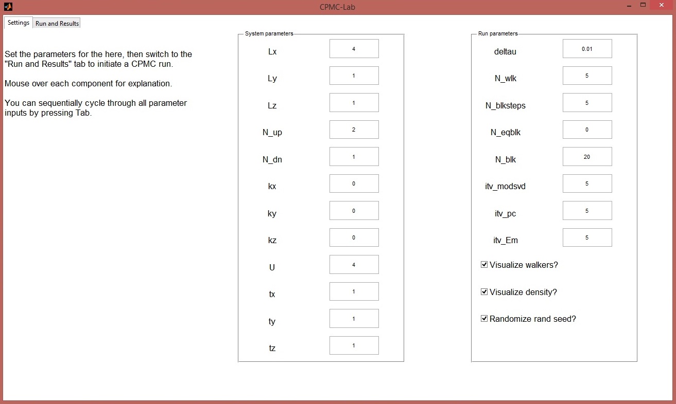
Figure 2: (Color online) The GUI tab that allows the user to set all the parameters of the calculation.

(a) With visualizations

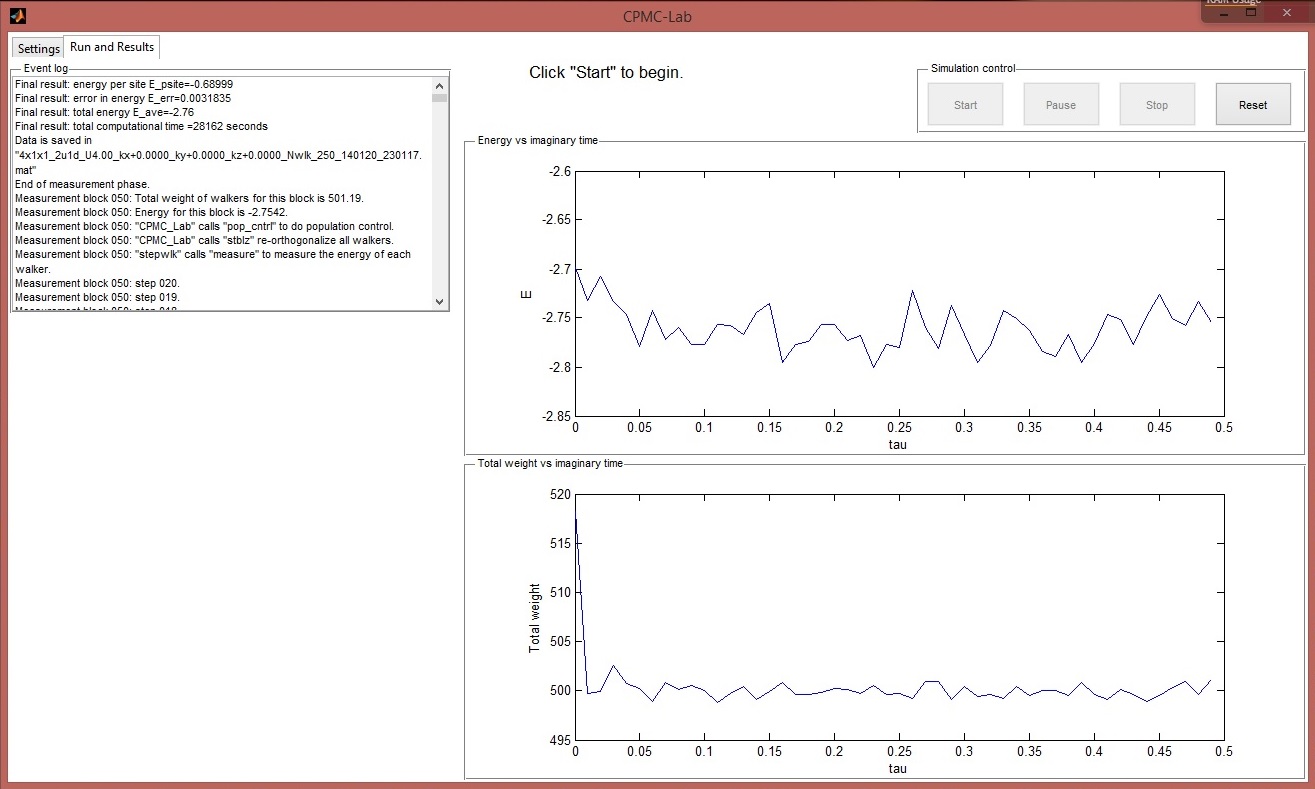
(b) Without visualizations

Figure 3: (Color online) The GUI for visualizing the calculation. These figures show (a) a detailed visualization mode which shows the walkers’ orbitals and electronic density, with the currently propagated walker highlighted in yellow, (b) the normal run mode with the detailed visualizations turned off.

The run could also be set in a more detailed visualization mode. The structure of the random walker orbitals is illustrated by plotting the orbital coefficients, along with the electronic “density” $\braket{n_{i\sigma}}$ for each spin at site $i$, defined as $\braket{n_{i\sigma}}=\braket{\phi_{k}}{\hat{n}_{i\sigma}}{\phi_{k}}$ for the $k$-th walker. Figure 3 shows this feature, in which a snapshot is highlighted for a four-site calculation.

IV.1 Files in the package

This package contains ten source files for the CPMC program, one GUI program, and two scripts as samples for running the program:

CPMC_Lab.m

is the main driver of the package. For every time step, it calls stepwlk.m to propagate the walkers. When appropriate, it calls measure.m to measure the energy, stlbz.m to re-orthonormalize the walkers or pop_cntrl.m to do population control. After the end of the random walk, it calculates the final average and standard error of the energy and saves the results to a file.

initialization.m

runs validation.m to conduct a basic check on the input parameters and initializes internal quantities, e.g. the total number of sites and electrons. It forms the free-electron trial wave function and creates the initial population of walkers.

validation.m

verifies the basic validity of user inputs, as mentioned above.

H_K.m

creates the one-body kinetic Hamiltonian.

stepwlk.m

carries out one step of the random walk by calling halfK.m, V.m and halfK.m again.

halfK.m

propagates a walker by $\mathrm{e}^{-\Delta\tau\hat{K}/2}$

V.m

carries out importance sampling site by site to select the auxiliary fields, and propagates a walker by $\mathrm{e}^{-\Delta\tau\hat{V}}$.

measure.m

computes the energy of a walker.

stblz.m

orthonormalizes walkers by the modified Gram-Schmidt algorithm.

pop_cntrl.m

carries out population control by a simple-combing method.

sample.m

is a script that allows users to set input parameters.

batchsample.m

is a script that loops over multiple sets of parameters.

GUI.m

launches the GUI of the package. It is a stand-alone file that is independent of all the other files in the package and contains all the subroutines of a QMC run.

IV.2 Exercises

Below is a list of suggested exercises. They are designed as a step-by-step guide for the reader to gain a basic familiarity with the code and learn the most essential features of a CPMC or AFQMC calculation. The concepts covered in the first few exercises are universal, such as auto-correlation time, statistical errors, equilibration time, Trotter errors, population control bias, and so on. It is essential to master them before any production runs. The other exercises are more open-ended. Their goal is to help the reader gain more insight and facilitate real applications. In the next Section, several example applications are shown.

IV.2.1 Running the sample script sample.m

The first assignment is to run a “sample.” To run the script sample.m, put all the files in this package directly under the current directory. Type “sample” (without quotes) and hit Enter to run the script. The main function CPMC_Lab will return the values of E_ave and E_err to the workspace, and save more detailed data in the ^*.mat file named by sampledatafile. The main function will also plot a figure of the energies from each measurement block, E(i_blk) vs. $\texttt{i\_blk}\times\texttt{N\_blksteps}\times\texttt{deltau}$.

Save the figure via the File menu and explain its behavior. Obtain a rough estimate for how much imaginary time is needed to equilibrate. This interval, $\tau_{\mathrm{eq}}$, corresponds to the input $\texttt{deltau}\times\texttt{N\_blksteps}\times\texttt{N\_eqblk}$. Now modify the parameters to include an “equilibration” phase. Do statistical analysis on the “measurement” phase or do a loop over different values of N_blksteps. We provide with the package a sample batch run script, batchsample.m, that loops over multiple sets of parameters. Determine the minimum length of each measurement block (N_blksteps) necessary to obtain uncorrelated results and a reliable estimate of the statistical error.

Now modify the parameters using the correct N_eqblk and N_blksteps for a few “standard” runs. Table 1 gives the exact energies for several systems ($U/t=4$) for comparison.

system		(kx,ky)	$\braket{K}$		$\braket{V}$		$E_{0}$
$2\times 1$	$1\uparrow 1\downarrow$	$(+0.0819,+0.0000)$	-3.	54222	1.	09963	-2.	44260
$4\times 1$	$2\uparrow 2\downarrow$	$(+0.0819,+0.0000)$	-3.	29161	1.	17491	-2.	11671
$8\times 1$	$4\uparrow 4\downarrow$	$(+0.0819,+0.0000)$	-7.	65166	3.	04575	-4.	60591
$2\times 4$	$3\uparrow 2\downarrow$	$(+0.0819,-0.6052)$	-13.	7778	1.	65680	-12.	1210
$3\times 4$	$3\uparrow 3\downarrow$	$(+0.02,0.04)$	-15.	2849	1.	29311	-13.	9918
$4\times 4$	$5\uparrow 5\downarrow$	$(0,0)$	-22.	5219	2.	94100	-19.	58094

Table 1: Parameters and exact results for sample runs.

IV.2.2 Controlling the basic run parameters

Let us next study the behaviors of the Trotter error and population control bias:

1. Run the code for a few different values of $\Delta\tau$ (deltau), e.g. 0.025, 0.05, and 0.1, and examine the convergence of the energies as a function of deltau. Note that the number of steps in each block, N_blksteps, the frequency of measurement, itv_em (and optionally itv_modsvd and itv_pc) should be adjusted to obtain comparable statistics.

2. Run the code for several values of population size (N_wlk), e.g. 10, 20, 40, and 80, and examine the population bias (systematic error vs. the population size). Note that with fewer walkers in the population, more blocks will be needed to get comparable statistical accuracy.

IV.2.3 Calculating E_K and E_V separately

The program only outputs the total ground state energy. The mixed-estimate for other observables is biased, as mentioned earlier. The standard way to calculate unbiased expectation values is to use the back-propagation technique (see Refs Zhang et al. (1995); Purwanto and Zhang (2004)). Let us calculate the kinetic energy E_K and the potential energy E_V in an alternative way. From the Hellman-Feynman theorem, we have

$$\texttt{E\_V}=\Braket{\psi(U)}{U\,\frac{\mathrm{d}H}{\mathrm{d}U}}{\psi(U)}=U\frac{\mathrm{d}E}{\mathrm{d}U}$$ (52)

Obtain $\frac{\mathrm{d}E}{\mathrm{d}U}$ by finite difference with three separate total energy calculations at $(U-\Delta U)$, $U$, and $(U+\Delta U)$ with a small $\Delta U$. Higher-order finite difference methods can also be used for more accurate results as illustrated in Section VI. Some exact results at $\texttt{U}=4$ are listed in Table 1 for comparison. For the two-dimensional system in the last three rows, obtain a result with sufficiently small statistical error bars to examine the systematic error from the constrained path approximation.

IV.2.4 The Hydrogen molecule

Let us study the system of two interacting fermions on two sites: $\texttt{N\_up}=1$, $\texttt{N\_dn}=1$, $\texttt{Lx}=2$ and $\texttt{Ly}=1$. We set $\texttt{tx}=1$ and $\texttt{kx}=0$ (ty and ky will be ignored when $\texttt{Ly}=1$). Study the properties of the system as the interaction strength U is varied (while keeping $t=1$). This can be viewed as a crude model (minimal basis) for breaking the bond in a H₂ molecule. As the distance between the two protons increases, the interaction strength $U/t$ increases.

1. Run the QMC code at different values of U and compare your results with the exact solution:

   $$E=\frac{1}{2}\left(U-\sqrt{U^{2}+64}\,\right)$$ (53)

2. Plot E_K and E_V vs. U. Explain their behaviors.

3. Obtain the double occupancy $\braket{n_{1\uparrow}n_{1\downarrow}}$ (see Section IV.2.3). From it, derive the correlation function $\braket{n_{1\uparrow}n_{2\downarrow}}$. Explain its behavior vs. U.

IV.2.5 Ground-state energy of a chain

Let us study the half-filled Hubbard model in one dimension and how the energy converges with respect to system size. Run the program for a series of lattice sizes (e.g. $2\times 1$, $4\times 1$, $6\times 1$, $8\times 1$, …), each averaging over a set of random twist angles kx. Plot the energy per site vs. $\texttt{1/L}^{2}$, and examine its convergence behavior. (In Section VI a detailed example is given.)

IV.2.6 Addition to the program: other correlation functions

Program in the mixed estimator of some observables, e.g. the one-body density matrix $\braket{c^{\dagger}_{i\sigma}c_{j\sigma}}$, the spin-spin correlation function $\braket{S_{i}S_{j}}$ (where $S_{i}=n_{i\uparrow}-n_{i\downarrow}$), and the charge-charge correlation function $\braket{(n_{i\uparrow}+n_{i\downarrow})(n_{j\uparrow}+n_{j\downarrow}})$. Calculate the mixed estimate for E_K and E_V and compare with the results from Sec. IV.2.3.

V Computational Speed

As mentioned in Section I, a major drawback of the Matlab package is that it is significantly slower than a standard production code written in FORTRAN or C. This is outweighed by the advantages in pedagogical value and in providing the clearest algorithmic foundation. From this foundation, the users could build a CPMC or phase-free AFQMC code tailored toward their own applications. As illustrated in the next section, significant applications can be carried with the present Matlab code as is.

Here we give some rough comparisons between the Matlab code and a production code in FORTRAN. To provide an idea of the timing difference, we describe two examples. For the calculation at $U=4$ in a $4\times 4$ lattice with 5 spin-$\uparrow$ and 5 spin-$\downarrow$ electrons (the same number of lattice sites as Figure 4), the FORTRAN code takes 1 minute to run on an Intel Core i7-2600 3.40 GHz processor, compared to 32 minutes for the Matlab code. Scaling up the system size to a $128\times 1$ lattice with 65 spin-$\uparrow$ and 63 and spin-$\downarrow$ electrons (the largest system in Figure 6), the FORTRAN code requires 186 minutes while the Matlab code takes 460 minutes. The parameters for both run are $\texttt{deltau}=0.01$, $\texttt{N\_wlk}=1000$, $\texttt{N\_blksteps}=40$, $\texttt{N\_eqblk}=10$, $\texttt{N\_blk}=50$, $\texttt{itv\_modsvd}=5$, $\texttt{itv\_pc}=40$ and $\texttt{itv\_Em}=40$.

Using OpenMP, Matlab can automatically speed up computations in a multi-core environment. Furthermore, Matlab users with Matlab’s Parallel Computing Toolbox installed can easily parallelize the code by distributing the propagation of individual walkers over multiple processor cores. This is done by 1) changing the main for loop in stepwlk.m into a parfor loop and 2) opening a pool of $n$ parallel Matlab workers with the command matlabpool(’open’,n) before the equilibration phase begins in CPMC_Lab.m.

The computational cost of the CPMC and phase-free AFQMC methods scales algebraically, roughly as the third power of system size. (Different pieces of the code scale as different combinations of $N$ and $M$.) The memory required to run CPMC-Lab is proportional to the product of (the basis size) $\times$ (the number of electrons) $\times$ (the number of random walkers). The random walkers are only loosely coupled. The approach is ideally suited for a distributed massively parallel environment Esler et al. (2008).

VI Illustrative Results

Figure 4 compares energy calculations by CPMC-Lab against exact diagonalization (ED) results for a one-dimensional 16-site Hubbard model with $5$ spin-$\uparrow$ and $7$ spin-$\downarrow$ electrons. The parameters of the run are $\texttt{N\_wlk}=5000$, $\texttt{deltau}=0.01$, $\texttt{N\_blksteps}=40$, $\texttt{N\_blk}=150$, $\texttt{N\_eqblk}=30$, $\texttt{itv\_pc}=5$, $\texttt{itv\_Em}=40$ and $\texttt{itv\_modsvd}=1$. The potential energy is obtained by the Hellman-Feynman method of Eq. (52), where the derivative $\frac{\mathrm{d}E}{\mathrm{d}U}$ is calculated using the five-point stencil. The kinetic energy is simply the difference between the total and potential energy.

In one-dimension, the CPMC method is exact. As seen in the figure, the agreement between CPMC and ED results is excellent. As the interaction strength $U$ increases, the kinetic energy also increases because more electrons are excited to occupy higher single-particle levels. The potential energy is non-monotonic as a consequence of two opposing tendencies. Double occupancy $\braket{n_{\uparrow}n_{\downarrow}}$ (shown in the inset) is rapidly reduced as the interaction is increased. On the other hand, the growing value of $U$ increases the potential energy linearly.

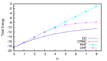
(a) Total energy

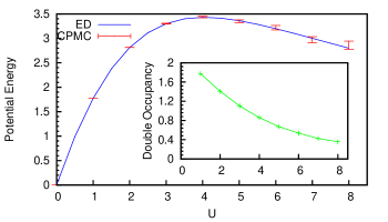
(b) Potential energy (inset: double occupancy $\braket{n_{\uparrow}n_{\downarrow}}$)

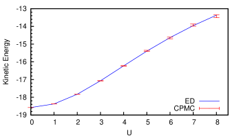
(c) Kinetic energy

Figure 4: (Color online) The total, potential and kinetic energies versus the interaction strength $U$ for a 16-site ring with $5$ spin-$\uparrow$ and $7$ spin-$\downarrow$ electrons. CPMC results (red error bars) are compared with exact diagonalization (ED) (blue solid curves). Restricted (cyan) and unrestricted (magenta) Hartree-Fock results have also been drawn for comparison in panel (a). The inset in panel (b) shows the double occupancy $\braket{n_{\uparrow}n_{\downarrow}}$.

We next compute ground-state properties of the one-dimensional Hubbard model in the thermodynamic limit. Since our QMC calculations are performed in finite-sized supercells, it is important to reduce finite-size effects and obtain better convergence as $M\to\infty$. In Figure 5, we show the calculated ground-state energy per site versus the supercell size at half-filling for $U=4$. We compare two sets of data, one with PBC ($\Gamma$-point) and the other with twist-averaging boundary condition (TABC) as discussed in Section II.6.3. In the TABC runs, each data point is obtained by averaging over random samples of the twist angle $\bm{\Theta}$. That is, the kx values are chosen randomly from the interval $(-1,1]$, corresponding to $\theta_{x}\in(-\pi,\pi]$. The number of kx points for each lattice size is chosen to keep the product $(\texttt{lattice size})\times(\texttt{number of kx values})$ roughly constant ($\sim 80$ in this case) while maintaining a minimum of 4 points.

In the PBC runs, we added a small twist angle kx whenever the electron configuration is open-shell in order to break the degeneracies in the single-particle energy levels (see Section II.6.3). The run parameters for this and subsequent results are identical to those used in Figure 4 except for $\texttt{N\_wlk}=1000$, $\texttt{itv\_pc}=40$ and $\texttt{itv\_modsvd}=5$.

The PBC data is seen to exhibit large finite-size effects, with a zig zag pattern reflecting differing trends for closed-shell and open-shell systems. We reiterate that this behavior is not from any numerical problem; rather it is the nature of the exact ground-state eigenvalue of the Hamiltonian for these finite supercells under PBC. The TABC data, on the other hand, is smooth and monotonic. As the supercell size increases, the two sets of data approach each other, and converge to the same limit. The best fit of the TABC data to a straight line is shown in the figure. The fit is given by $E_{0}/M=-0.57361-0.63192/M^{2}$, leading to a thermodynamic value of $-0.5736(1)$, to be compared to the exact result of $-0.573729$ from the Bethe ansatz Lieb and Wu (1968).

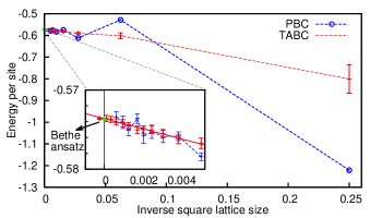
Figure 5: (Color online) Ground-state energy per site vs. inverse square lattice size for half-filled one-dimensional lattices at $U=4$. Results from PBC (blue) and TABC (red) are shown. The lattice size in PBC ranges from 2 to 40 and those in TABC are from 2 to 128. The red solid line in the inset is the best fit of the TABC data (for lattice sizes 4 to 128) while the dashed blue line is to guide the eye. The inset shows a closeup view (from 12 to 128 sites) of the convergence to the thermodynamic limit. The exact result is shown in green for comparison. For clarity, the error bar of the intercept in the inset is offset to the left of the green symbol for exact result.

We next compute the spin and charge excitation gaps. The spin gap is defined as the energy difference between the present system and that with one spin flipped:

$$\Delta_{\mathrm{s}}=E_{0}\left(N_{\uparrow}+1,N_{\downarrow}-1\right)-E_{0}\left(N_{\uparrow},N_{\downarrow}\right)\,,$$ (54)

where $E_{0}\left(N_{\uparrow},N_{\downarrow}\right)$ is the total ground-state energy for a finite supercell with $N_{\uparrow}$ spin-$\uparrow$ and $N_{\downarrow}$ spin-$\downarrow$ electrons.

Figure 6 shows the result of the spin gap for the one-dimensional Hubbard model at half-filling, for $U=4$, as a function of inverse lattice size. TABC is used in these calculations, choosing a random set of twist values to calculate each total energy in Eq. (54). The parameters of the run are identical to those in Figure 4.

As the lattice size increases, the calculated spin gap converges smoothly. A linear fit to all the data yields an asymptotic value of $\Delta_{\mathrm{s}}=0.0036(80)$, consistent with the Haldane conjecture of a zero spin gap Haldane (1983a, b).

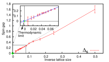
Figure 6: (Color online) The calculated spin gap vs. inverse lattice size for one-dimensional Hubbard model at half-filling, $U=4$. The red dashed line is drawn to guide the eye. The inset shows a closeup view of the convergence from 12 to 128 sites. The blue solid line is a linear fit of the data for lattice sizes 8 to 128. For clarity, the error bar of the intercept in the inset is offset to the left of the vertical axis at $1/M=0$.

The charge gap is defined by the addition and removal energy:

$$\Delta_{\mathrm{c}}=E_{0}\left(N_{\uparrow}+1,N_{\downarrow}\right)+E_{0}\left(N_{\uparrow}-1,N_{\downarrow}\right)-2\,E_{0}\left(N_{\uparrow},N_{\downarrow}\right)\,,$$ (55)

where in the present case $N_{\uparrow}=N_{\downarrow}=M/2$. We also calculate, alternatively

$$\Delta_{\mathrm{c}}^{\prime}=E_{0}\left(N_{\uparrow}+1,N_{\downarrow}+1\right)-E_{0}\left(N_{\uparrow},N_{\downarrow}\right)-U\,,$$ (56)

which we expect to give a consistent result based on the analytic result relating the chemical potentials to $U$ Lieb and Wu (1968). The results of the calculated charge gap at $U=4$ are shown in Figure 7.

As the lattice size increases from 2 to 128 (right to left), both types of charge gap converge toward a finite value. A linear fit to the data of $\Delta_{\mathrm{c}}$ yields a charge gap of $1.266(21)$ in the thermodynamic limit, consistent with the exact analytic result of $1.28673$ Lieb and Wu (1968).

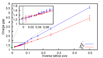
Figure 7: (Color online) The calculated charge gap vs. inverse lattice size for the one-dimensional Hubbard model at half-filling, $U=4$. The lattice size ranges from 2 to 128. The two sets of data are obtained according to $\Delta_{\mathrm{c}}^{\prime}$ (blue) and $\Delta_{\mathrm{c}}$ (red), respectively. The dashed curves in the main figure are drawn to guide the eye. The inset shows a closeup view at larger supercell sizes. The red and blue solid lines represent linear fits to the corresponding subsets of data with lattice sizes 16 to 128. The exact result of $1.28673$ in the thermodynamic limit is indicated in green for comparison. For clarity, in the inset, the error bars for the two intercepts are offset to the left of the green symbol for exact result.

VII Summary

In this paper we described CPMC-Lab, an open-source Matlab program for studying the many-body ground state of Hubbard-like models in any dimension, and for learning the constrained-path and phase-free auxiliary-field Monte Carlo methods. The package illustrates the constrained-path Monte Carlo method, with a graphical interface. The ground-state energy is calculated using importance sampling and implementing the algorithmic details of a total energy calculation. This tool allows users to experiment with various model and run parameters and visualize the results. It provides a direct and interactive environment to learn the method and study the code with minimal overhead for setup. Furthermore, it provides a foundation and template for building a CPMC or phase-free AFQMC calculation for essentially any interacting many-fermion system with two-body interactions, including ab initio calculations in molecules and solids.

VIII Acknowledgment

We gratefully acknowledge support by the US National Science Foundation Grant nos. DMR-1006217 and DMR-1409510 (H.N., J.X., and S.Z.), by the Department of Energy under grant no. DE-SC0008627 (H.S. and S.Z.) and by Reed College under the Summer Experience Award (H.N.). Computing support was provided by a DOE INCITE Award and from William and Mary’s SciClone cluster.

Appendix A Some useful Matlab commands

• Tab completion is available in the Matlab command window for the names of functions and scripts (either built-in, on the search path or in the current directory) and variables in the current workspace.

• Ending a command with semicolon suppresses its output.

• To display the value of the variable variablename:

  ⬇

  variablename

• To display a brief description and the syntax for functionname in the command window:

  ⬇

  help functionname

• To call a function:

  ⬇

  [out1,out2,...]=myfunc(in1,in2,...)

• To run the script scriptname:

  ⬇

  scriptname

• To set display format to long (15 decimal places) instead of the default short (4 decimal places):

  ⬇

  format long

• To load the variables from a *.mat file into the workspace:

  ⬇

  load filename.mat

  or double click the *.mat file or select Import Data from the workspace menu

• To remove all variables from the workspace:

  ⬇

  clear

• To generate an $m\times n$ matrix containing pseudorandom values drawn from the standard uniform distribution on $(0,1)$:

  ⬇

  rand (m, n)

• To create a new individual figure window on the screen:

  ⬇

  figure

• To close all the figure windows:

  ⬇

  close all

• To plot each column in the (real) matrix Ydata versus the index of each value:

  ⬇

  plot(Ydata)

• To plot each column in the matrix Ydata versus Xdata:

  ⬇

  plot(Xdata,Ydata)

• To plot each vector in Yn versus the corresponding vector Xn on the same axes:

  ⬇

  plot(X1,Y1,X2,Y2,...,Xn,Yn)

• To plot Ydata versus Xdata with symmetric error bars 2*Err(i) long:

  ⬇

  errorbar(Xdata,Ydata,Err)

• To hold the plot so that subsequent plotting commands add to the existing graph instead of replacing it:

  ⬇

  hold all

• To put a title string at the top-center of the current axes:

  ⬇

  title(’string’)

• To label the x-axis:

  ⬇

  xlabel(’string’)

  and similarly for the y-axis

References

- Zhang (2013) S. Zhang, in Emergent Phenomena in Correlated Matter Modeling and Simulation, vol 3, edited by E. Pavarini, E. Koch, and U. Schollwock (Forschungszentrum Julich, 2013) p. 15.1, iSBN 978-3-89336-884-6. Free online at http://www.cond-mat.de/events/correl13.
- Zhang et al. (1997) S. Zhang, J. Carlson, and J. E. Gubernatis, Phys. Rev. B 55, 7464 (1997).
- Chang and Zhang (2008) C.-C. Chang and S. Zhang, Phys. Rev. B 78, 165101 (2008).
- Zhang and Krakauer (2003) S. Zhang and H. Krakauer, Phys. Rev. Lett. 90, 136401 (2003).
- Al-Saidi et al. (2006) W. A. Al-Saidi, S. Zhang, and H. Krakauer, The Journal of Chemical Physics 124, 224101 (2006).
- Chang and Zhang (2010) C.-C. Chang and S. Zhang, Phys. Rev. Lett. 104, 116402 (2010).
- Shi and Zhang (2013) H. Shi and S. Zhang, Physical Review B 88, 125132 (2013).
- Purwanto et al. (2009a) W. Purwanto, H. Krakauer, and S. Zhang, Phys. Rev. B 80, 214116 (2009a).
- Ma et al. (2013) F. Ma, S. Zhang, and H. Krakauer, New J. Phys. 15, 093017 (2013).
- Purwanto et al. (2011) W. Purwanto, H. Krakauer, Y. Virgus, and S. Zhang, J. Chem. Phys. 135, 164105 (2011).
- Martin (2004) R. M. Martin, Electronic Structure: Basic theory and practical methods (Cambridge University Press, Cambridge, UK, 2004).
- Gonze et al. (2009) X. Gonze, B. Amadon, P.-M. Anglade, J.-M. Beuken, F. Bottin, P. Boulanger, F. Bruneval, D. Caliste, R. Caracas, M. Côté, T. Deutsch, L. Genovese, P. Ghosez, M. Giantomassi, S. Goedecker, D. Hamann, P. Hermet, F. Jollet, G. Jomard, S. Leroux, M. Mancini, S. Mazevet, M. Oliveira, G. Onida, Y. Pouillon, T. Rangel, G.-M. Rignanese, D. Sangalli, R. Shaltaf, M. Torrent, M. Verstraete, G. Zerah, and J. Zwanziger, Computer Physics Communications 180, 2582 (2009).
- Valiev et al. (2010) M. Valiev, E. Bylaska, N. Govind, K. Kowalski, T. Straatsma, H. V. Dam, D. Wang, J. Nieplocha, E. Apra, T. Windus, and W. de Jong, Computer Physics Communications 181, 1477 (2010).
- Kalos et al. (1974) M. H. Kalos, D. Levesque, and L. Verlet, Phys. Rev. A 9, 2178 (1974).
- Ceperley and Kalos (1979) D. M. Ceperley and M. H. Kalos, in Monte Carlo Methods in Statistical Physics, edited by K. Binder (Springer-Verlag, Heidelberg, 1979) Chap. 4, pp. 145–194.
- Shi et al. (2014) H. Shi, C. A. Jimenez-Hoyos, R. Rodriguez-Guzman, G. E. Scuseria, and S. Zhang, Phys. Rev. B 89, 125129 (2014).
- Hamann and Fahy (1990) D. R. Hamann and S. B. Fahy, Phys. Rev. B 41, 11352 (1990).
- Zhang (1999) S. Zhang, Phys. Rev. Lett. 83, 2777 (1999).
- Rubenstein et al. (2012) B. M. Rubenstein, S. Zhang, and D. R. Reichman, Phys. Rev. A 86, 053606 (2012).
- Hirsch (1985) J. E. Hirsch, Phys. Rev. B 31, 4403 (1985).
- Umrigar et al. (1993) C. J. Umrigar, M. P. Nightingale, and K. J. Runge, J. Chem. Phys. 99, 2865 (1993).
- Purwanto and Zhang (2004) W. Purwanto and S. Zhang, Phys. Rev. E 70, 056702 (2004).
- Zhang and Kalos (1991) S. Zhang and M. H. Kalos, Phys. Rev. Lett. 67, 3074 (1991).
- Zhang (2000) S. Zhang, Computer Physics Communications 127, 150 (2000).
- Lin et al. (2001) C. Lin, F. H. Zong, and D. M. Ceperley, Phys. Rev. E 64, 016702 (2001).
- Xu et al. (2011) J. Xu, C.-C. Chang, E. J. Walter, and S. Zhang, Journal of Physics: Condensed Matter 23, 505601 (2011).
- Purwanto et al. (2009b) W. Purwanto, S. Zhang, and H. Krakauer, The Journal of Chemical Physics 130, 094107 (2009b).
- Sorella (2011) S. Sorella, Phys. Rev. B 84, 241110 (2011).
- Carlson et al. (2011) J. Carlson, S. Gandolfi, K. E. Schmidt, and S. Zhang, Phys. Rev. A 84, 061602 (2011).
- Calandra Buonaura and Sorella (1998) M. Calandra Buonaura and S. Sorella, Phys. Rev. B 57, 11446 (1998).
- Zhang et al. (1995) S. Zhang, J. Carlson, and J. E. Gubernatis, Phys. Rev. Lett. 74, 3652 (1995).
- Esler et al. (2008) K. P. Esler, J. Kim, D. M. Ceperley, W. Purwanto, E. J. Walter, H. Krakauer, S. Zhang, P. R. C. Kent, R. G. Hennig, C. Umrigar, M. Bajdich, J. Kolorenc, L. Mitas, and A. Srinivasan, Journal of Physics: Conference Series 125, 012057 (15pp) (2008).
- Lieb and Wu (1968) E. H. Lieb and F. Y. Wu, Physical Review Letters 20, 1445 (1968).
- Haldane (1983a) F. Haldane, Physics Letters A 93, 464 (1983a).
- Haldane (1983b) F. D. M. Haldane, Phys. Rev. Lett. 50, 1153 (1983b).