Abstract

We construct a world model consisting of matter fields living in 4 dimensional spacetime and a gravitational field living in 11 dimensional spacetime. The seven hidden dimensions are compactified within a radius estimated by reproducing the particle - wave characteristic of diffraction experiments. In the presence of matter fields the gravitational field develops localized modes with elementary excitations called gravonons which are induced by the sources (massive particles). The final world model treated here contains only gravonons, gravitons and a scalar matter field. The gravonons are localized in the environment of the massive particles which generate them. The solution of the Schrödinger equation for the world model yields matter fields which are localized in the 4 dimensional subspace. The localization has the following properties: (i) There is a chooser mechanism for the selection of the localization site. (ii) The chooser selects one site on the basis of minor energy and gravonon differences between the sites, which at present cannot be controlled experimentally and therefore let the choice appear statistical. (iii) The changes from one localization site to a neighbouring one take place in a telegraph-signal like manner. (iv) The times at which telegraph like jumps occur dependent on subtleties of the gravonon structure which at present cannot be controlled experimentally and therefore let the telegraph-like jumps appear statistical. (v) The fact that the dynamical law acts in the configuration space of fields living in 11 dimensional spacetime lets the events observed in 4 dimensional spacetime appear non-local. In this way the phenomenology of Copenhagen quantum mechanics is obtained without the need of introducing the process of collapse and a statistical (probabilistic) interpretation of the wave function. Operators defining observables need not be introduced. The known commutation relations for observables in 4 dimensions can be derived but they are no prerequisite for interpreting experiments. All experimental findings are explained in a deterministic way as a consequence of the time development of the wave function in configuration space according to Schrödinger’s equation without the need of introducing a statistical interpretation.

Keyword: Emerging quantum mechanics, Copenhagen quantum mechanics , quantum field theory, collapse, entanglement to gravitons, weak field gravity, chooser, particle localization, wave - particle duality

1 Introduction

The problem of whether quantum mechanics, including the postulated concept of random collapses, provides a real representation of the world or whether it implies just a probabilistic interpretation of experimental data is still discussed controversially. Whereas Penrose suggests that collapse is a dynamics arising in a natural way from gravity penrose1 -penrose6 , Omnes claims that decoherence solves the problem and, hence, objectification in quantum mechanics is a non-existent problem omnes . Kiefer and Joos maintain that the dynamical collapse models invoking gravity may be simply drowned by environmental decoherence and hence are to be considered as ”excess baggage” kiefer1 -kieferjoos . As far as locality is concerned, d’Espagnat contends that decoherence theory does not reconcile physics with the objective existance of phenomena (strong realism) despagnat1 ; despagnat2 . Dürr and Teufel maintain that decoherence does not create the facts of our world, but rather produces a sequence of fapp-redundancies, which physically increase or stabilize decoherence. They believe that physical theory should describe the behaviour of real objects, located in physical space duerrbook . In the present paper we report a theory which is in the spirit of quantum realism.

As is well known and well accepted, the Schrödinger equation evolves a state, which qualifies as representing real world, into a state which is a superposition of real world states and as such does not qualify as a real world state. To handle this problem von Neumann vonNeumann introduced a second dynamics which is not unitary and serves as reduction on real world states. This second dynamics is referred to as collapse or state vector reduction and cannot presently be described by a mathematical theory. We refer to this state of quantum theory as Copenhagen Quantum Mechanics (CQM).

In recent years there have been attempts to construct theories where Copenhagen quantum mechanics and/or quantum field theory emerge in the low energy (infrared) limit of a (higher-dimensional) theory which is capable of combining quantum mechanics and general relativity. Superstring theory and/or M-theory string are the most well-known examples. According to a different theory developed by ’t Hooft the fundamental laws valid at the Planck scale are derived from Newton’s law, but are different. In this theory Copenhagen quantum mechanics emerges as the low energy limit due to a chaotic (dissipative) dynamics (loss of information) with a set of attractors operating during the development of the system from the Planck scale to the microscopic (atomic) scale. Classical variables can assume any arbitrary value out of a continuum while quantum states are discrete thooft1 -thooft3 . Inspired by ’t Hooft’s idea, Blasone et al. blasone show that the combined evolution of two classical, dissipative harmonic oscillators results in a linear harmonic quantum oscillator with a zero point energy.

Adler proposes that Copenhagen quantum mechanics is an emergent phenomenon arising from a deeper level of dynamics via an extension of classical dynamics to non-commuting matrix variables, with cyclic permutation inside a trace used as the basic calculational tool. Copenhagen quantum mechanics is then shown to emerge as the statistical thermodynamics of this underlying theory, with the canonical commutation-anticommutation relations derived from a generalized equipartition theorem. State vector reduction and probabilistic interpretation of Copenhagen quantum mechanics are then argued to follow from Brownian motion like corrections to the Schrödinger equation adler ; adler1 . Smolin considers classical matrix models with an explicit stochastic noise giving rise to quantum behaviour smolin .

Biró et al. biro demonstrate that a classical (Euclidean) field theory living in five dimensions can behave in the infrared limit like a quantum system, if it is only observed in four dimensions. Hadley argues that the fundamental logic of Copenhagen quantum mechanics results from general relativity. In his theory elementary particles are not separate objects living in 4 dimensional spacetime, but rather constituents (local deformations) of spacetime. General relativity contains past and future in a deterministic manner. The statistical character of Copenhagen quantum mechanics is then a consequence of the missing knowledge of the future hadley .

A different approach is to modify the Schrödinger equation in such a way that the collapse dynamics is included in its solution. These are the so called collapse models GRW ; Pearlecoll . For a detailed review see ref. Pearlecoll .

It is often stated that Copenhagen quantum mechanics explains all known phenomena and experimental findings and that experimental hints to a different physics are not available haag . This is clearly not true. With the advent of experimental techniques, which provide data with time resolution and spatial resolution on the atomic scale of the dynamics of chemical and physical processes on solid surfaces in a non-destructive way, Copenhagen quantum mechanics is challenged. Within Copenhagen quantum mechanics collapse of the total wave function might be postulated as the process leading to the localization of adsorbed atoms and molecules on solid surfaces, as they are imaged in experiments with the low-temperature scanning tunnelling microscope eiglerXe ; lauhonho . The two-dimensional periodicity of the solid surfaces means delocalization of the wave function in two dimensional Bloch waves resulting from the time development of the wave packets according to Schrödinger’s equation. It would imply that an initially localized adparticle should after some time be observed anywhere on equivalent sites on the surface with equal probability. This is, however, never observed. An extension of Copenhagen quantum mechanics by including the system and the environment is often considered under the heading of decoherence theory. According to this theory localization via interaction, ”permanent measurement” by environmental particles (phonons, tomonagons, photons, plasmons, etc.) is suggested. But it cannot be the explanation either. This is so because at low temperatures the available environmental excitations have very long wavelengths compared to the size of the adsorbed particles. Furthermore, when adsorbed particles jump between two adsorption sites, the movement occurs as telegraph-signal like jumps and not as the smooth Rabi oscillations predicted by Schrödinger’s equation meyer . The diffusion rates in the quantum diffusion regime of the same adsorbate on similar metal surfaces, measured in different experiments, differ by several orders of magnitude lauhonho ; gomer . Copenhagen quantum mechanics, with the coupled dynamics of the adsorbate motion and the substrate phonons taken into account, provides results, which drastically differ by nearly nine orders of magnitude from the experimental diffusion rates wahn1997 . The desorption reaction of CO, induced by tunnelling electrons in the scanning tunnelling microscope COdesorption , can be explained only by assuming that the tunnelling electron is transiently localized in the close vicinity of the adsorbate doydrakCOdesorp . The survival of metastable atoms in interaction with adsorbate covered solid surfaces ertl presents a further problem, which cannot be resolved within Copenhagen quantum mechanics. The survival probability of metastable atoms He^∗ on a metal surface, covered with CO, is attenuated compared to the deexcitation probability in a scattering experiment between a beam of He^∗ and CO in the gas phase, which is unexpected and not explained within Copenhagen quantum mechanics upto now. In ref. doyHe-COscattering an understanding has been suggested, based on the different dimensionality of the scattering continua in the gas phase and on the solid surface. This has been termed the dimensionality effect doyphyrevb and is in the spirit of the theory developed here.

Recently, a programmable quantum annealing machine has been built which uses quantum effects to minimize a cost function aepli . The question has been raised whether the behaviour of this D-wave computer dwavesys can be described by classical statistical mechanics, an approach called simulated annealing, or whether Copenhagen quantum mechanics has to be invoked in order to explain the operation of D-wave. It has been established experimentally by Chiorescu et al. chiorescu that a single qubit loses coherence within nanoseconds, i.e. within a few nanoseconds the behaviour of a single qubit can no longer be described by Copenhagen quantum mechanics. In Ramsey interferometry experiment a $\frac{\pi}{2}$ microwave pulse initializes Rabi oscillations between the macroscopic supercurrent in the flux qubit in two reverse directions, which are interpreted as oscillating probability for occupation of one current state. The envelope of the oscillations of this probability decays, providing a ”coherence time” of one current state of the order of 20 nanoseconds. These observations are interpreted to demonstrate that within nanoseconds the behaviour of a single qubit can no longer be described by Copenhagen quantum mechanics.

On the other hand, Johnson et al. show that in a macroscopic system of an eight-qubit chain the quantum annealing of the system at low temperature results in quantum tunnelling in the global energy minimum, with a temperature independent freezing time johnson . Furthermore the experiment of Dickson et al. dwave using 16 qubits of a superconducting quantum processor and quantum annealing with the help of applied transverse magnetic fields shows that, even with annealing time eight orders of magnitude longer than the time, determined for the decay of the oscillations described above, the system behaves as predicted by Copenhagen quantum mechanics. Classical models do not reproduce the experimental results.

We applied the theory presented in this contribution successfully to explain why does the D-wave computer operate as a quantum computer over minutes, despite that the effects of the thermal environment are on a timescale of nanoseconds. An understanding can be provided in the framework of the present theory unpublished .

It appears that the localization of quantum particles via entanglement to environmental continua of high density of states is a necessary condition for various reactions on solid surfaces. Particle localization in a collapse process, as suggested in Copenhagen quantum mechanics is, however, not the result of the solution of Schrödinger’s equation or of any well defined dynamics. The examples from the previous paragraph illustrate that on a nanoscale level on solid surfaces there are dynamical processes which cannot be accounted for by Copenhagen quantum mechanics. In all cases mentioned, entanglement with an environment obviously plays a role. However, the environmental excitations usually discussed in the context of these low temperature experiments, for instance phonons, tomonagons, plasmons etc., are not capable to localize atoms or electrons on a solid surface because of their long wavelength. A new explanation is needed.

We develop a theory where Copenhagen quantum mechanics emerges from a quantum field theory, which treats gravitation in eleven spacetime dimensions in the weak field limit. Entanglement to soft modes in the hidden spatial dimensions leads to particle localization, which is a necessary condition for the processes on the atomic scale, listed in the previous paragraph. Changes of localization sites occur as a telegraph like dynamics with entanglement to low frequency modes and in the limit of vanishing interaction strength. Non-locality in four spacetime dimensions is implicit in the theory. It also is capable of describing and explaining the experiments on solid surfaces mentioned beforehand, which was found impossible within Copenhagen quantum mechanics.

There exist many attempts to account for the effects of gravity on a quantum system by modifying Schrödinger’s equation including stochastic attractive Newtonian gravitational fields in 4 dimensional spacetime diosi3 -hughston or introducing a nonlinear ”Schrödinger-Newton” equation penrose1 ; diosi3 . The interpretation is based on the tendency of the off-diagonal elements of the reduced density matrix of a quantum system in interaction with the external gravitational field to attenuate, and is assumed to imply transition to classical and random behaviour. Instead, gravitation has been suggested as the origin of the noise field in collapse models Pearlecoll . Penrose’s intensive attempts also suggest gravitation as the origin of collapse penrose1 -penrose6 . With the purpose to describe localization and transition of the quantum mechanical superposition of states to classical states, even the decay mecahanism is often postulated penrose1 ; diosi3 . Within the framework of continuous spontaneous reduction models GRW Pearle and Squires interpret the classical scalar field, which causes collapse, as the gravitational curvature scalar, however, gravity is treated semiclassically pearle . In the work of Anastopoulos the gravitational field is considered as leading to classical behaviour, however, not for microscopic particles anast . Spacetime fluctuations due to stochastic backgrounds of gravitational waves lamine or metric fluctuations breuer have also been suggested to lead to unavoidable transition of quantum particles to classical behaviour.

The aspects of Copenhagen quantum mechanics are shown in this paper to emerge from entanglement due to an extremely localized and weak interaction between matter fields and a massless boson field of high mode density. The exact form of the Lagrangian for the interacting fields will be developed in sections 3 to 5. In section 2 we investigate the structure of a theory based on an extremely local and weak interaction with a high density continuum in 11 dimensional spacetime. This includes compactification of the hidden dimensions (section 2.1.1), determination of the density of states (section 2.1.2) and the special kind of solution not obtainable in perturbation theory (sections 2.2 and 2.2.1). The properties of the solution are exemplified for the case of diffraction from nano lattices. In sections 6 and 7 the ontology of our Emerging Quantum Mechanics (EQM) is set in relation with that of Copenhagen and Bohmian quantum mechanics.

2 The structure of a deterministic Schrödinger theory in 11 dimensional spacetime including weak field gravitation

As mentioned in the introduction a possible theory for the unification of general relativity and quantum mechanics is superstring theory and/or M-theory string . The equations of superstring theory are mathematically consistent only, if the strings move in 10 dimensional space. According to M-theory spacetime can besides one-dimensional strings also contain branes of various dimensions. Strings can be restricted to subspaces of spacetime, if they are bound to branes. The physical laws depend on the geometry and dimensions of the branes and the hidden dimensions.

2.1 Hidden dimensions

First we briefly summarize the way we think about this subject. A single hidden dimension can only have the shape of a circle. More extra dimensions can have a variety of shapes (called topologies) such as spheres, tori, connected tori, etc. differing in length and diameter. This results in a gigantic number of possible geometries. In addition there are parameters describing the positions of the branes and the fluxes around the tori. Each configuration of branes and hidden dimensions has a different energy. If there are no fields in 4 dimensional spacetime this corresponds to the vacuum energy. For a given three dimensional brane the geometry of the hidden dimensions is determined by minimizing this vacuum energy. The multitude of possible geometries results in the so called landscape of string theory. Our universe has to correspond to a minimum on the landscape with a relatively small vacuum energy, the geometry of branes and hidden dimensions corresponding to our universe is, however, unknown. For the purpose of this investigation we assume the simplest possible case, namely a flat 3-dimensional brane and a seven dimensional sphere representing the hidden dimensions. All known fields except for the gravitational field are assumed to live only on the three dimensional brane. Except for the existence of such a three dimensional brane and the spherically compactified hidden dimensions, no other properties of superstring theory and/or M-theory are needed.

2.1.1 Compactification of the hidden dimensions

The basic idea of how Copenhagen quantum mechanics emerges in our theory is that the gravitational interaction provides a chooser that guides a diffracted matter field to a particular site on the screen. Assume the simple case that a point like source emitting the matter field is exactly in the center of a three dimesional sphere of radius 1 meter. The area of the sphere is then $4\pi$ m${}^{2}\approx 16\pi 10^{20}$ bohr${}^{2}\approx 5\cdot 10^{21}$ bohr². Assuming an area of the lattice unit cell of the screen of 25 bohr², there will be $2\cdot 10^{20}$ sites on the screen where the matter field could localize ("collapse"). The idea is that the sites are fully equivalent but vary slightly in energy and geometry. A realistic estimate for this is a variation in energy of $\approx 10^{-3}$ eV and a variation in geometry of $\approx 10^{-1}$ bohr.

The average spacing between two adjacent energy levels is $10^{-3}$ eV$/10^{20}$ sites$=10^{-23}$ eV. If the only criterion is energy then the chooser has to distinguish energy levels on a scale of $10^{-23}$ eV in order to select a single site. Analogously the average deviation between two similar geometries will be $10^{-1}$ bohr$/10^{20}$ sites$=10^{-21}$ bohr. If the only criterion is geometry then the chooser has to distinguish geometry on a scale of $10^{-21}$ bohr in order to select a single site. If we assume that the chooser is sensitive to geometric differences of $10^{-5}$ bohr then $10^{16}$ sites would be available for a choice. This means then that the chooser should distinguish on an energy scale of $10^{-3}$ eV$/10^{16}$ sites$=10^{-19}$ eV in order to select a single site.

The consequence is that the interaction energy between a quantum of the matter field and a site on the screen should be of this order of magnitude. A larger interaction energy cannot lead to site selection. A significantly smaller interaction energy would mean that either very many quanta of the matter field have to be emitted from the source, before a "collapse" can be registered, or that it would take months or years before a quantum can be registered on the screen. Both cases violate strongly the experimental findings.

The required interaction strength is much weaker than any kind of electrodynamical, chemical or van der Waals interaction. This means that coupling to phonons or electron - hole pairs, i.e. "measurement by the environment", is not capable of describing the "collapse" or measurement process which is at the heart of the so called wave - particle duality. On the other hand the required interaction strength is much stronger than gravitational interaction in 4 dimensional spacetime. Consider two protons at a distance of r=6 bohr and mass $M=10^{4}$ a.u. Their gravitational interaction energy is $GM^{2}/r\approx 10^{-33}$ eV, where we inserted a value of $G=10^{-40}$ atomic units for Newton’s gravitational constant. This is 14 orders of magnitude smaller than required. The only possibility for obtaining the required order of magnitude for the interaction energy appears to be a gravitational field in 11 dimensional spacetime with compactified hidden dimensions.

The gravitational potential provided by a pointlike mass $M$ in 4 dimensional spacetime is:

$$V_{grav}^{(4)}(r)=-\frac{GM}{r}$$ (1)

In 11 dimensional spacetime (10 space dimensions) the gravitational potential is:

$$V_{grav}^{(11)}(r)=-\frac{G^{(11)}M}{\pi^{7}r^{8}}$$ (2)

The gravitational law eq. (2) cannot be valid for large separations $r$ as this would violate the experimentally verified classical law eq. (1). Therefore the hidden dimensions are rolled up (compactified) to a diameter $2a$ so that at large distances the separation in the hidden dimensions never exceeds $2a$. Equating the classical and the 11 dimensional gravitational law at large distances, we obtain

$$-\frac{GM}{r}=-\frac{G^{(11)}M}{(2a\pi)^{7}r}\rightarrow G^{(11)}=(2a\pi)^{7}G$$ (3)

This choice makes the two laws eq. (1) and eq. (2) agree at separations larger than $2a$. Inserting eq. (3) in eq. (2) yields at $r=1$ bohr:

$$V_{grav}^{(11)}(r=1)=-GM(2a)^{7}$$ (4)

This means that at $r=1$ bohr the gravitational interaction is $(2a)^{7}$ times stronger than predicted by the classical law eq. (1).

The dependence of $G^{(11)}$ on the compactification radius is then:

a	$G^{(11)}/\pi^{7}$
$10^{4}$	$10^{-10}$
$10^{3}$	$10^{-17}$
$10^{2}$	$10^{-24}$
$10$	$10^{-31}$

From the selection criterion described above we require $\frac{G^{(11)}M}{\pi^{7}r^{8}}\approx 10^{-20}$ atomic units at $r=6$ bohr and $M=10^{4}$, hence $\frac{G^{(11)}M}{\pi^{7}6^{8}}\approx\frac{G^{(11)}10^{4}}{\pi^{7}10^{6}}\approx\frac{G^{(11)}}{\pi^{7}}*10^{-2}\approx 10^{-20}$ which implies $\frac{G^{(11)}}{\pi^{7}}\approx 10^{-18}$. For our chooser we would therefore need a compactification radius of roughly $10^{3}$ bohr. This is enormously larger than the Planck length. A chooser needs large extra dimensions. In the theory of Arkani-Hamed et al. it is also claimed that the hidden dimensions need not be compactifed on the Planck scale, they can be as large as a fraction of a millimeter or even infinite add4 .

2.1.2 Graviton mode density

The chooser can only work, if gravitons are available at an energy separation which is of the order of the gravitational interaction strength for any kind of matter field quantum. This is only possible, if the density of graviton modes is sufficiently large. The density of graviton modes has been calculated in ref. dice2010-more . Due to its importance the argument is repeated here. The calculation runs parallel to the evaluation of the mode density in the electromagnetic case. We expand the gravitational radiation field in the eigenmodes of resonators with fixed frequency, polarization, and field distribution. Although the selection of modes is in principle arbitrary, the most popular expansion uses the eigenmodes of rectangular boxes with perfectly reflecting walls. The mirrors at position 0 and $a$ impose the boundary conditions that the field vanishes at those positions. The eigenmodes have field distributions that vary with ${\rm sin}(n\pi x/a)$, where $n$ is the mode number, $x$ the spatial variable and $a$ the separation of the two mirrors. The spatiotemporal variation of the field is

$$F_{n}={\rm sin}(n\pi x/a){\rm e}^{i\omega_{n}t}$$ (5)

The wave number $k=(n\pi/a)$ determines the angular frequency $\omega_{n}=\frac{n\pi{\rm c}}{a}$. The one dimensional density of modes in $k$-space is

$$\rho_{k}=\frac{a}{\pi}.$$ (6)

Using the dispersion relation for gravitons $\epsilon_{\kappa}=\kappa{\rm c}$, with ${\rm c}$ the velocity of light,
$\kappa=\sqrt{k_{1}^{2}+k_{2}^{2}+k_{3}^{2}+k_{4}^{2}+...+k_{d}^{2}}$ and $d$ the dimension of gravitational $k$-space, we write for the graviton mode density

$$\rho_{grav}(E)=\sum_{\kappa}\delta(E-\epsilon_{\kappa})=\int{\rm d}^{d}\kappa\rho_{\kappa}^{d}\delta(E-\epsilon_{\kappa}).$$ (7)

Transforming to spherical coordinates $\eta$ one obtains zwiebach ;

$$\rho_{grav}(E)=\int{\rm d}\eta\eta^{d-1}\delta(E-\epsilon_{\kappa})\rho_{\kappa}^{d}\frac{\pi^{d/2}}{\Gamma(1+\frac{d}{2})}.$$ (8)

Specializing to 10 spatial dimensions and substituting ${\rm d}\eta={\rm d}\epsilon/{\rm c}$ one obtains

$$\rho_{grav}(E) = \frac{1}{{\rm c}}\frac{\pi^{5}}{\Gamma(1+5)}\rho_{\kappa}^{d}\int{\rm d}\epsilon\frac{\epsilon^{d-1}}{{\rm c}^{d-1}}\delta(E-\epsilon)$$ (9)

$$= \frac{E^{9}}{{\rm c}^{10}}\frac{\pi^{5}}{5!}(\frac{L}{\pi})^{3}(\frac{a}{\pi})^{7}$$ (10)

where $L$ is the normalization length of the macroscopic three dimensional space and $a$ is the normalization length of the hidden dimensions.

The density of states for the two dimensional movement of an adparticle of mass $M$ is $\rho_{2D}=\frac{2ML^{2}}{\pi}$ which is of the order of $10^{17}$ for a proton. Therefore the relationship between the mode density of gravitons at energy $E$ and the two dimensional adparticle motion is

$$\frac{\rho_{grav}}{\rho_{2D}}=\frac{\frac{E^{9}}{{\rm c}^{10}}}{2M}\frac{\pi^{5}}{5!}\frac{La^{7}}{\pi^{9}}\approx 10^{34}.$$ (11)

For the wave vector of the graviton we assumed $\kappa\approx 10$ bohr^-1, which corresponds to a wave length of 1 bohr ($\lambda=2\pi/\kappa\approx 1$ bohr), and $L\approx 10^{7}$ bohr. With the choice $a\approx 10^{4}$ bohr and $M=2000$ a.u., the graviton energy is of order of $\epsilon_{\kappa}\approx 10^{3}$ Hartree.

In conclusion the graviton continuum appears infinitely dense compared to the continua describing any particle motion in our three dimensional space.

2.2 Characteristics of the solution

In quantum field theory the standard way of solving a problem is via perturbation theory (Feynman diagrams). This approach does not work at all in our case. The reason is that the solution we are looking for appears in the limit of very small (vanishing) interaction strength (cf. section 2.1.1). Expanding in terms of powers of a coupling constant, which then tends to zero, yields zero in every order and for the final summation. This problem is known in quantum field theory, where topological (soliton) solutions appear for coupling constant tending to zero (cf. e.g. Zee zee who refers to this situation as "breaking the shackles of Feynman diagrams"). In our case the entanglement between the matter field and gravitons becomes maximal in the (mathematical) limit, where the interaction strength $V_{grav}$ tends to zero while at the same time the graviton density of states $\rho_{grav}$ tends to $\infty$ so that $V_{grav}\rho_{grav}$ stays non-zero and finite.

The method we have to pursue is solving the Schrödinger equation in configuration space. In quantum field theory the wave function becomes a wave functional, i.e. it depends directly on the fields. Considering for illustrative purposes only two boson fields, the scalar matter field $\phi(t,x_{1},x_{2},x_{3})$ and the gravitational field $\zeta(t,x_{1},x_{2},...,x_{10})$, we have to solve the Schrödinger equation

$$i\frac{\partial}{\partial t}\Psi\left(\phi(t,x_{1},x_{2},x_{3}),\zeta(t,x_{1},x_{2},...,x_{10})\right)$$

$$={\rm H}\Psi\left(\phi(t,x_{1},x_{2},x_{3}),\zeta(t,x_{1},x_{2},...,x_{10})\right).$$ (12)

Reasonable solutions can be obtained by adapting techniques, which have been developed in theoretical quantum chemistry under the heading of "configuration interaction" (CI).

Consider the set of fields $\{\phi^{n}\zeta^{m}\}$ forming a Hilbert space. Expanding the fields in modes ${\phi_{\alpha}}$ and ${\zeta_{\beta}}$:

$$\phi = \sum_{\alpha=1}^{\infty}C_{\alpha}\phi_{\alpha}$$ (13)

$$\zeta = \sum_{\beta=1}^{\infty}D_{\beta}\zeta_{\beta}$$ (14)

we write the wave functional in Dirac notation as

$$\mid\Psi\rangle=\sum_{\{n_{\alpha}\},\{n_{\beta}\}}A_{\{n_{\alpha}\}\{n_{\beta}\}}\otimes_{\alpha=1}^{\infty}\mid n_{\alpha}\rangle\otimes_{\beta=1}^{\infty}\mid n_{\beta}\rangle$$ (15)

with

$$\mid n_{\alpha}\rangle = (\phi_{\alpha}(x))^{n_{\alpha}}$$ (16)

$$\mid n_{\beta}\rangle = (\zeta_{\beta}(x))^{n_{\beta}}$$ (17)

$$\otimes_{\alpha=1}^{\infty}\mid n_{\alpha}\rangle = \mid n_{1}\rangle\otimes\mid n_{2}\rangle\otimes\mid n_{3}\rangle\otimes\mid n_{4}\rangle\otimes...$$ (18)

$$\{n_{\alpha}\} = n_{1}n_{2}n_{3}n_{4}n_{5}...$$ (19)

The time dependence of the modes ${\phi_{\alpha}}$ and ${\zeta_{\beta}}$ is just an arbitrary phase factor which can be set equal to unity. The time dependence arising from the relative phases is then contained in $A_{\{n_{\alpha}\}\{n_{\beta}\}}$. A scalar product $\langle\{n_{\alpha}\}\{n_{\beta}\}\mid\{n_{\gamma}\}\{n_{\delta}\}\rangle$ is defined by

$$\langle\{n_{\alpha}\}\{n_{\beta}\}\mid\{n_{\gamma}\}\{n_{\delta}\}\rangle=\prod_{\alpha,\beta,\gamma,\delta=1}^{\infty}\delta_{n_{\alpha}n_{\gamma}}\delta_{n_{\beta}n_{\delta}}$$ (20)

We refer to $\mid\{n_{\alpha}\}\{n_{\beta}\}\rangle$ as a (field) configuration. Introducing creation and annihilation operators $a_{\alpha}^{+}$, $a_{\alpha}$, $b_{\beta}^{+}$, $b_{\beta}$ in the usual way, one writes for the field configuration

$$\mid\{n_{\alpha}\}\{n_{\beta}\}\rangle=\prod_{\alpha=1}^{\infty}\prod_{\beta=1}^{\infty}(a_{\alpha}^{+})^{n_{\alpha}}(b_{\beta}^{+})^{n_{\beta}}\mid\{n_{\alpha}=0\}\{n_{\beta}=0\}\rangle.$$ (21)

The solution of the time dependent Schrödinger equation is

$$\mid\Psi(t)\rangle=e^{-i{\rm H}t}\mid\Psi(t=0)\rangle$$ (22)

where ${\rm H}$ is the Hamiltonian derived in sections 3 to 5. The time dependent amplitude becomes

$$A_{\{n_{\alpha}\}\{n_{\beta}\}}(t)=\langle\{n_{\alpha}\}\{n_{\beta}\}\mid e^{-i{\rm H}t}\mid\Psi(t=0)\rangle.$$ (23)

The initial functional $\mid\Psi(t=0)\rangle$ can be expanded in the field configurations:

$$\mid\Psi(t=0)\rangle=\sum_{\{n_{\gamma}\}\{n_{\delta}\}}B_{\{n_{\gamma}\}\{n_{\delta}\}}\mid\{n_{\gamma}\}\{n_{\delta}\}\rangle.$$ (24)

For the amplitude one obtains then

$$A_{\{n_{\alpha}\}\{n_{\beta}\}}(t)=\sum_{\{n_{\gamma}\}\{n_{\delta}\}}B_{\{n_{\gamma}\}\{n_{\delta}\}}\langle\{n_{\alpha}\}\{n_{\beta}\}\mid e^{-i{\rm H}t}\mid\{n_{\gamma}\}\{n_{\delta}\}\rangle.$$ (25)

The configuration interaction matrix elements in the last equation have to be evaluated using the hamiltonian ${\rm H}$ which consists of terms like $h_{\alpha\beta}a_{\alpha}^{+}a_{\beta}$, $v_{\gamma\delta}b_{\gamma}^{+}b_{\delta}$, $h_{\alpha\beta\gamma\delta}a_{\alpha}^{+}a_{\beta}b_{\gamma}^{+}b_{\delta}$ and their hermitian conjugate. The operation $a_{\kappa}^{+}a_{\lambda}b_{\mu}^{+}b_{\nu}\mid\{n_{\alpha}\}\{n_{\beta}\}\rangle$ is defined by eq. (21).

2.2.1 Telegraph signals ("quantum jumps")

Whereas the theory is relativistic, i.e., Lorentz invariant, the interesting solutions emerge in the non-relativistic limit. If the time dependent wave functional is calculated along the lines just outlined, one finds that configurations $\mid\{n_{\alpha}=1\}\{n_{\beta}=0\}\rangle$ restricted to four dimensional spacetime ("three dimensional configurations") become heavily entangled with configurations living essentially in eleven dimensional spacetime. The reason is that due to the high density of "gravonon configurations" (i.e. configurations where gravonons in the hidden dimensions have been excited, cf. section 3.2) a particular four dimensional configuration will always be practically degenerate with gravonon configurations and, as it is well known, the Schrödinger equation will mix degenerate configurations even for vanishingly small interaction strength.

In the problem of diffusion of an adsorbed particle on a solid surface the Hamiltonian has been chosen as doyenDICE2012 ; drakovaDICE2012 :

$${\rm H} = {\rm H}_{gas\;atom}+{\rm H}_{graviton}+{\rm H}_{gas\;atom-graviton}$$ (26)

$$= E_{g_{1}}n_{g_{1}}+E_{g_{2}}n_{g_{2}}+E_{w_{1}}n_{w_{1}}+E_{w_{2}}n_{w_{2}}+\sum_{i=1}^{2}V_{loc}^{g_{i}}(a^{+}_{g_{i}}a_{w_{i}}+a^{+}_{w_{i}}a_{g_{i}})$$

$$+ \sum_{i=1}^{2}\{\varepsilon_{grav_{i}}b^{+}_{grav_{i}}b_{grav_{i}}+\sum_{k}\varepsilon_{k_{i}}b^{+}_{k_{i}}b_{k_{i}}$$

$$+ \sum_{k}[V_{grav,w_{i}}n_{w_{i}}b^{+}_{grav_{i}}b_{k_{i}}+V_{w_{i},grav_{i}}n_{w_{i}}b^{+}_{k_{i}}b_{grav_{i}}]\}.$$

The meaning of the symbols is: $n_{g_{i}},n_{w_{i}}$: gas particle field strength in the vibrationally ground and excited (parallel to the surface) core movement states and in the "warp resonance" where interaction with the gravonons occurs; $a^{+}_{i},a_{j}$: creation and annihilation operators for the gas particle field in the respective core movement states; $V_{loc}^{g_{i}}$: interaction strength between a gas particle state and the warp resonance; $\varepsilon_{grav_{i}},\varepsilon_{k_{i}}$: energy quanta of local and continuum gravonon fields; $b^{+}_{grav_{i}},b_{grav_{i}}$: creation and annihilation operators for the local gravonon field; $b^{+}_{k_{i}},b_{k_{i}}$: creation and annihilation operators for the continuum gravonon field; $V_{grav,w_{i}}$: interaction between the gas particle and the gravonons within the warp resonance.

The field configurations taken into account are the following:

$$\{n_{\alpha}\}=n_{g1}n_{g2}n_{w1}n_{w2}$$ (27)

with $n_{gi}=0,1$, $n_{wi}=0,1$ for $i=1,2$.

$$\{n_{\beta}\}=n_{k1}n_{k2}$$ (28)

with $n_{ki}=0,1,...,\infty$ for $i=1,2$.

The solution of the Schrödinger equation for this Hamiltonian results in the adparticle being fixed near a particular substrate atom as long as the excited gravonons are moving around in the large hidden dimensions. If after the recurrence time the gravonons return to the four dimensional brane where they have been excited, the adparticle is suddenly free to leave this site. When arriving at a neighbouring site the adparticle will excite gravonons here and will be captured to this new site as long as the excited gravonons are moving around in the large hidden dimensions. This leads to the telegraph signal like adsorbate movement, which is observed in experiment. A calculation of this movement within the present theory is depicted in fig. 1. The analytical derivation of why and how telegraph signal like changes in the state of a quantum system, entangled with gravonons in the environment, occur, is presented in ref. arxive .

2.2.2 The chooser mechanism ("collapse")

The scattering of a matter field from a double slit and the "wave - particle duality" observed in these experiments is in our theory interpreted as follows. If there is a site on the screen which is energetically degenerate with the initial wave functional $\mid Q0\rangle=\mid\Psi(t=0)\rangle$ the configuration $\mid K\kappa_{proj}\rangle$ with the scalar matter field $\phi$ having significant strength on this site will get strongly entangled with the degenerate gravonon configurations. As the excitations of the gravonons in the hidden dimensions depend on the matter field being extremely localized near the chosen site the matter field strength cannot drift away as long as the excited gravonons are moving around in the large hidden dimensions. If this takes time long enough for other physical-chemical processes to be initiated, it will result in an experimentally detectable event. Such an event would be called "collapse" in the framework of Copenhagen quantum mechanics.

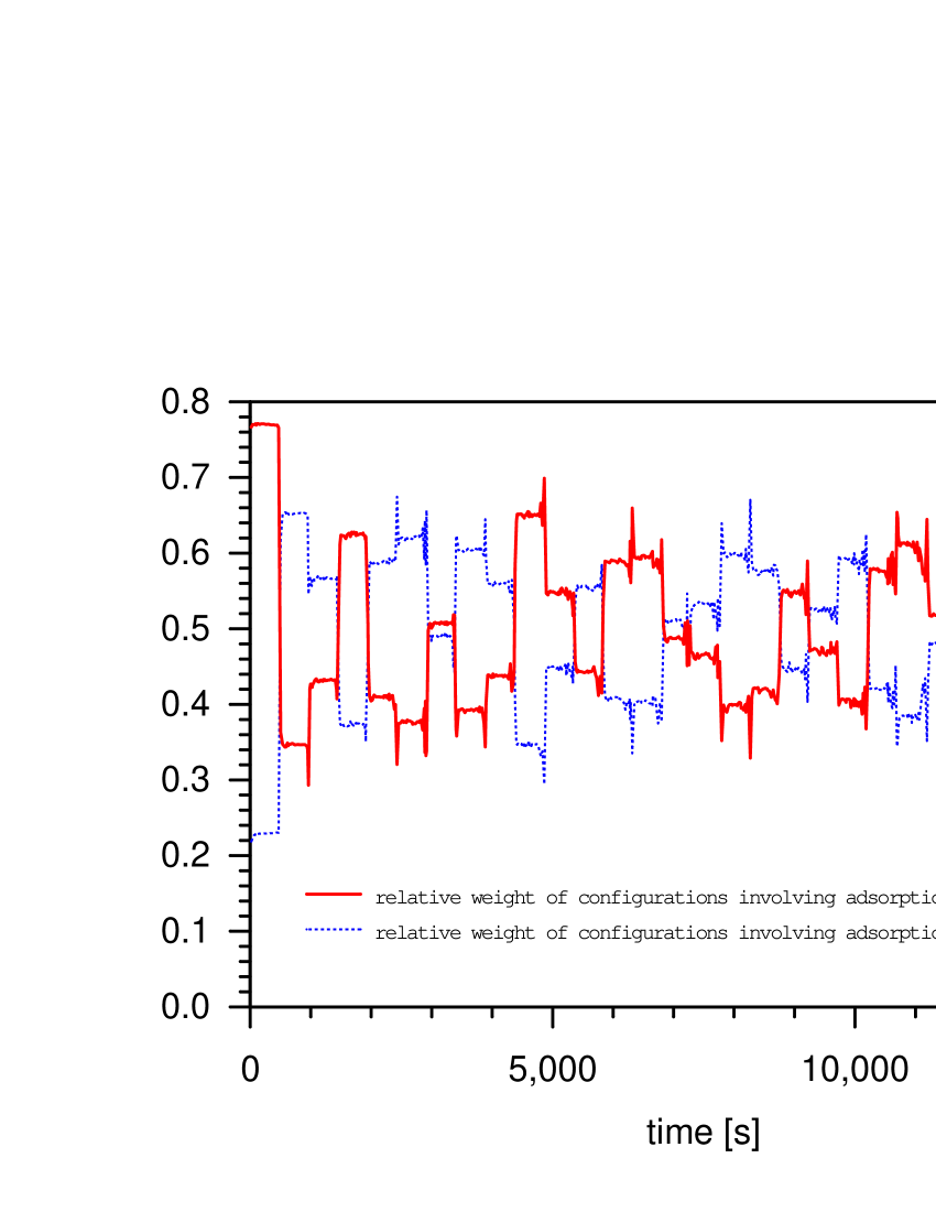
Figure 1: Adsorbate telegraph-signal-like quantum jumps between two adsorption sites as a function of time obtained as a solution of the Schrödinger equation . The entanglement with the gravonon field is included. The quantity plotted is the squared coefficient of the field configurations containing gravonons summed over site 1 and site 2, respectively, with a full and a dashed curve.

To treat this situation theoretically in a simplified manner we set up the Hamiltonian ${\rm H}$ in matrix form

	$\mid Q0\rangle$	$\mid R0\rangle$	$\mid K\kappa_{proj}\rangle$
$\langle Q0\mid$	$0$	$V$	0
$\langle R0\mid$	$V$	0	W
$\langle K\kappa_{proj}\mid$	0	W	0

Figure 2 illustrates the many-particle states involved and their interactions.

Figure 2: Field configurations and their interactions: $\mid Q0\rangle=\mid Q\rangle\otimes\mid 0_{grav}\rangle$ initial field configuration with the gravitational field in the ground state and the matter field in the source; $\mid R0\rangle=\mid R\rangle\otimes\mid 0_{grav}\rangle$ with the matter field localized on the screen but not yet entangled with the gravonons, which are in the ground state; $\mid K\kappa_{proj}\rangle$ with the matter field localized on the screen and a gravonon state projected out of the gravonon band $\{\mid\kappa\rangle\}$ according to the criterion of strongest interaction.

$\mid R0\rangle=\mid R\rangle\otimes\mid 0_{grav}\rangle$ is a state where the matter field is localized on the screen but not yet entangled with the gravonons. In the state $\mid K\kappa_{proj}\rangle$ the matter field experiences the interaction with the gravitational field. All three states are degenerate at energy $E=0$ which defines the energy zero. The interaction $V$ allows the matter field to penetrate into the localized state $\mid R0\rangle$ on the screen and $W$ is the potential connecting $\mid R0\rangle$ to the resonance $\mid K\kappa_{proj}\rangle$ where gravitational interaction becomes important.

Diagonalizing the Hamiltonian leads to the characteristic equation

$${\rm det}(E-{\rm H})=E^{3}-(W^{2}+V^{2})E=0$$ (29)

which has the solutions $E_{o}=0$, $E_{\pm}=\pm\sqrt{W^{2}+V^{2}}$. Only the eigenstate $\mid 00\rangle$ of energy zero is of interest in the following. It has the coefficients

$$C_{Q0} = \frac{W}{\sqrt{V^{2}+W^{2}}}$$ (30)

$$C_{R0} = 0$$ (31)

$$C_{K\kappa_{proj}} = \frac{V}{\sqrt{V^{2}+W^{2}}}.$$ (32)

In the limit where the coupling to the gravonons becomes very weak ($\frac{W}{V}\rightarrow 0$) $C_{Q0}=0$ and $C_{K\kappa_{proj}}=1$. The coefficients of the "zero-state" $\mid 00\rangle$ in the eigenstates of the total system become then approximately

$$\langle 00\mid K\kappa+\rangle = \langle 00\mid{\rm G}^{+}(\epsilon_{\kappa})(W_{grav}+V+W)\mid K\kappa\rangle$$ (33)

$$\approx \langle K\kappa_{proj}\mid{\rm G}^{+}(\epsilon_{\kappa})(W_{grav}+V+W)\mid K\kappa\rangle$$ (34)

$$= \langle K\kappa_{proj}\mid{\rm G}^{+}(\epsilon_{\kappa})\mid K\kappa_{proj}\rangle\langle K\kappa_{proj}\mid W_{grav}\mid K\kappa\rangle$$ (35)

$$= G_{K\kappa_{proj}}^{+}(\epsilon_{\kappa})W_{\kappa}$$ (36)

where ${\rm G}^{+}$ is the Green operator, $W_{grav}$ is the gravitational potential, $G_{K\kappa_{proj}}^{+}=\langle K\kappa_{proj}\mid{\rm G}^{+}\mid K\kappa_{proj}\rangle$ and $W_{\kappa}=\langle K\kappa_{proj}\mid W_{grav}\mid K\kappa\rangle$. $\mid\kappa\rangle$ is one of the states in the gravonon band, generating $\mid\kappa+\rangle$ after the interaction with the matter field is included. $\epsilon_{\kappa}$ is the eigenenergy of the eigenstate $\mid Kk+\rangle$. We have here applied the Lippmann-Schwinger equation lippschwi to construct the eigenstates $\mid K\kappa+\rangle$. The Green function $G_{K\kappa_{proj}}^{+}$ has the form

$$G_{K\kappa_{proj}}^{+}(\epsilon_{\kappa})=\frac{1}{\epsilon_{\kappa}-\alpha(\epsilon_{\kappa})+i\Gamma(\epsilon_{\kappa})}$$ (37)

where $\alpha$ and $\Gamma$ are the real and imaginary parts of the self-energy, respectively, with

$$\Gamma(\epsilon_{k}) = \pi\sum_{\kappa}\mid W_{\kappa}\mid^{2}\delta(E-\epsilon_{\kappa})$$ (38)

$$= \pi\frac{U^{2}}{\Delta}\;\;{\rm i}{\rm f}\mid\epsilon_{k}\mid<\Delta$$ (39)

The last line indicates an approximation where $W_{\kappa}=\frac{U}{\sqrt{N}}$ is non-zero and energy independent over an energy range of length $\Delta$ and zero otherwise. $N$ is the number of gravonons in the energy interval $\Delta$. Defining the density $\rho_{\epsilon}$ of gravonon levels at $\epsilon_{\kappa}=0$

$$\frac{\rho_{\epsilon}}{N} = \frac{1}{\Delta}$$ (40)

$$= -\frac{1}{\pi}{\rm I}{\rm m}{\rm G}^{+}_{K\kappa_{proj}}$$ (41)

$$= \frac{1}{\pi\Gamma}$$ (42)

yields $\Delta=\pi\Gamma$. In order to study the time dependence due to the coupling to the gravonons we start from the formal solution of the time dependent Schrödinger equation

$$\mid\Psi(t)\rangle = e^{-i{\rm H}t}\mid 00\rangle$$ (43)

$$= \sum_{\kappa}{\rm e}^{-i\epsilon_{\kappa}t}\mid K\kappa+\rangle\langle K\kappa+\mid 00\rangle$$

$$= \sum_{\kappa}{\rm e}^{-i\epsilon_{\kappa}t}\mid K{\kappa}+\rangle G_{K\kappa_{proj}}^{-}(\epsilon_{\kappa})W_{\kappa}$$

$$= \sum_{\kappa}{\rm e}^{-i\epsilon_{\kappa}t}\mid K{\kappa}+\rangle\frac{W_{\kappa}}{\epsilon_{\kappa}-\alpha(\epsilon_{\kappa})-i\Gamma(\epsilon_{\kappa})}$$

where we assumed $W_{\kappa}$ to be real. For the projection $\langle K\kappa_{proj}\mid\Psi(t)\rangle$ we obtain:

$$\langle K\kappa_{proj}\mid\Psi(t)\rangle=\sum_{\kappa}{\rm e}^{-i\epsilon_{\kappa}t}\langle K\kappa_{proj}\mid K\kappa+\rangle\frac{W_{\kappa}}{\epsilon_{\kappa}-\alpha(\epsilon_{\kappa})-i\Gamma(\epsilon_{\kappa})}.$$ (44)

From eq. (38), with $W_{\kappa}$ assumed to be independent of $\epsilon_{\kappa}$, we have:

$$\langle K\kappa_{proj}\mid K{\kappa}+\rangle W_{\kappa}=\frac{U}{N}.$$ (45)

Inserting in eq. (44) we obtain

$$\langle K\kappa_{proj}\mid\Psi(t)\rangle=\frac{U}{N}\sum_{\kappa}\frac{{\rm e}^{-i\epsilon_{\kappa}t}}{\epsilon_{\kappa}-\alpha(\epsilon_{\kappa})-i\Gamma(\epsilon_{\kappa})}$$ (46)

where $\langle K\kappa_{proj}\mid K{\kappa}+\rangle=\frac{1}{\sqrt{N}}$ is assumed to be independent of $\epsilon_{\kappa}$. We have to emphasize at this point that the summation index $\kappa$ is not the graviton wave vector. The sum runs over the energy levels of the gravonon states (cf. section 3.2). The sum in eq. (46) can therefore be transformed into an integral by writing

$$\langle K\kappa_{proj}\mid\Psi(t)\rangle=\frac{U}{N}\int_{-\infty}^{\infty}{\rm d}\epsilon_{\kappa}\rho_{\epsilon}\frac{{\rm e}^{-i\epsilon_{\kappa}t}}{\epsilon_{\kappa}-\alpha(\epsilon_{\kappa})-i\Gamma(\epsilon_{\kappa})}.$$ (47)

($\rho_{\epsilon}$, the level density of gravonon states, is constant according to eq. (40).) We assume $\alpha$ and $\Gamma$ to be independent of energy. The time dependent wave functional $\mid\Psi(t)\rangle$ and its component involving the localized matter state $\mid K\rangle$ is then obtained by integration yielding gradshteyn

$$\langle K\kappa_{proj}\mid\Psi(t)\rangle=i\pi\frac{U}{N}\rho_{\epsilon}{\rm e}^{-\Gamma t}=i\pi\frac{U}{\Delta}{\rm e}^{-\Gamma t},$$ (48)

where in the weak interaction limit we assumed $\alpha\rightarrow 0$ and $\rho_{\epsilon}=\frac{N}{\Delta}$ (eq. 40).

In order to clarify the complete character of the state $\mid\Psi(t)\rangle$ we have also to calculate its projections on $\mid R0\rangle$, $\mid Q0\rangle$ and $\mid K\lambda+\rangle$.

$$\langle R0\mid K\kappa+\rangle = \langle R0\mid G^{o}(W_{grav}+V+W)\mid K\kappa+\rangle$$ (49)

$$= G^{o}_{R0}\langle R0\mid(W_{grav}+V+W)\mid K\kappa+\rangle$$ (50)

$$= G^{o}_{R0}\langle R0\mid(W_{grav}+V+W)\mid K\kappa_{proj}\rangle\langle K\kappa_{proj}\mid K\kappa+\rangle$$ (51)

$$= \frac{W}{\sqrt{N}}\lim_{\epsilon\rightarrow 0}\frac{1}{\epsilon_{\kappa}+i\epsilon}$$ (52)

$$= \frac{W}{\sqrt{N}}\left[{\cal P}(\frac{1}{\epsilon_{\kappa}})-i\pi\delta(\epsilon_{\kappa})\right]$$ (53)

Using this in eq. (43) yields then with $W_{k}=U/\sqrt{N}$ and $\rho_{\epsilon}=N/\Delta$

$$\langle R0\mid\Psi(t)\rangle=\pi\frac{UW}{\Delta(\Gamma-i\alpha)}$$ (54)

$$\langle Q0\mid K\kappa+\rangle = \langle Q0\mid G\mid K\kappa_{proj}\rangle\langle K\kappa_{proj}\mid W_{grav}\mid K\kappa\rangle$$ (55)

$$= \frac{U}{\sqrt{N}}\langle Q0\mid G\mid K\kappa_{proj}\rangle$$ (56)

Inserting the Born series

$$G=G^{o}+\sum_{n=0}^{\infty}(G^{o}(V+W)G^{o})^{n}$$ (57)

one has

$$\langle Q0\mid K\kappa+\rangle = \frac{W}{\sqrt{N}}\sum_{n=0}^{\infty}(\langle Q0\mid G^{o}\mid Q0\rangle\langle Q0\mid V\mid R0\rangle\langle R0\mid G^{0}\mid K\kappa_{proj}\rangle)^{n}$$ (58)

which is zero at every order and hence $\langle Q0\mid K\kappa+\rangle=0$. Requiring unitarity and setting $\alpha=0$ one gets

$$\sum_{\lambda}\mid\langle K\lambda+\mid\Psi(t)\rangle\mid^{2} = 1-\mid\langle K\kappa_{proj}\mid\Psi(t)\rangle\mid^{2}-\mid\langle R0\mid\Psi(t)\rangle\mid^{2}-\mid\langle Q0\mid\Psi(t)\rangle\mid^{2}$$ (60)

$$= 1-\pi^{2}\left[\frac{U^{2}}{\Delta^{2}}e^{-2\Gamma t}+(\frac{UW}{\Delta\Gamma})^{2}+0\right]$$

$$\approx 1-e^{-2\Gamma t}-\frac{W^{2}}{U^{2}}$$ (61)

The last line is valid, because from eq. (38) $\frac{U^{2}}{\Delta}=\Gamma/\pi$ and $\Delta=\pi\Gamma$ (eq. 40).

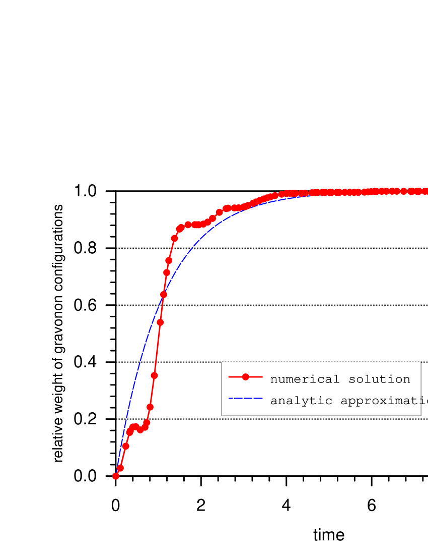
Figure 3: The chooser at work: the numerical solution of the model of section 2.2.2 in the basis displayed in fig. 2 (full curve) in comparison to the analytical approximation eq. (61) (dashed curve).

Neglecting off-shell components, the initial state $\mid Q0\rangle$, by propagating through the nano lattice (or double slit), becomes the state $\mid 00\rangle$, which for weak gravitational interaction strength merges into the state $\mid K\kappa_{proj}\rangle$ and then is completely extinguished with time according to eq. (48). The whole field strength is captured in the states $\{\mid K{\kappa}+\rangle\}$, representing a localized matter field, strongly entangled with gravonon states, which live mainly in the hidden dimensions.

In fig. 3 the sum of the weights of the gravonon configurations (squared coefficients) in the wave functional shows that as the system, displayed in fig. 2, develops with time the weight of the field configurations with gravonon components increases, tending to 1. This means that the matter field is localized and a ”collapse” occurs on a single site $\mid K\rangle$ where the entanglement with the gravonons is effective. The oscillations in the exact numerical calculation arise, as the off-shell states with $E_{\pm}$ are also mixed in because of the finite energy spread of the gravonons.

In the present theory the experimentally detectable event is uniquely determined already at the moment of the emission of the matter field quantum from the source, because exact energetical degeneracy is needed and, as outlined in section 2.1.1, due to the weakness of the interaction there is only one site of suitable energy available on the screen.

2.2.3 Beables and non-locality

Following Bell bell ; Bell2 we exclude the notion of observables in favour of beables. The beables bell ; Bell2 of our theory are the field configurations where matter fields extremely localized in three dimensional space are entangled to gravonons moving in 11 dimensional spacetime. These beables emerge in the non-relativistic limit within a preferred Lorentz frame, corresponding to the rest frame of the investigated system, the laboratory and the experimenter.

Unlike Copenhagen quantum mechanics where few "observables" have to be chosen from an infinite set of hermitian operators by using criteria which lie outside the realm of Copenhagen quantum mechanics, namely by being found suitable for the interpretation of experiments, the beables which define measurement are uniquely defined within our theory, based on the Schrödinger equation.

It is interesting that our definition of a beable is compatible with Kant’s ideas about observations kant . According to Kant, knowledge rests on our sensual contact with the world, and our sensibility has its limits. The sensual limits Kant called the forms of intuition. He argued that the forms are space and time auyang .

The intuitive nature of our beables is in marked contrast to the artificial constructs which are sometimes necessary in Copenhagen quantum mechanics to define e.g. the measured expectation values of the electromagnetic field (see auyang , note 43).

The transition from configuration space to the three dimensional space experienced by the experimenter is unambiguously provided by the localization in 3 dimensional space of the matter field. As the beables emerge (in the non-relativistic limit) from a solution of the Schrödinger equation in the (high-dimensional) configuration space, the beables, as observed in three dimensional space, clearly exhibit non-locality, i.e., beables can appear simultaneously at different points in 3 dimensional space, if we describe the 3 dimensional space in the rest frame.

The fact that the beables only emerge in the non-relativistic limit and are neither defined nor empirically accessible for relative velocities (between experimenter and physical event), approaching the velocity of light, resolves the apparent paradox of "real collapses in Minkowski spacetime" callender . According to this paradox beables which appear simultaneously in one Lorentz frame appear at different times in another Lorentz frame. This difference in time is noticeable only, if the relative velocity of the two Lorentz frames approaches the velocity of light.

As both the exerimenter and the physical event which she is to observe consist of beables, according to the present theory the beables representing "collapses" and/or "quantum jumps" are not empirically accessible as such by the experimenter, if the physical event moves with a velocity near to the velocity of light relative to the experimenter. This is associated with the fact that our theory does not contain "collapses" or "quantum jumps" as additional processes compared to Copenhagen quantum mechanics, where these processes occur in all Lorentz frames immediately. In our theory collapses are replaced by deterministic localization processes which can occur and switch in a telegraph signal like way. These telegraph signal like processes occur in the rest frame of the experiment within a very short time, but they are not immediate. If the observer moves with a high velocity relative to the experimental setup, the telegraph signal like processes slow down and can no longer represent "collapses" or "quantum jumps" of the Copenhagen quantum mechanics type.

This is the well established time dilatation which is present in our Lorentz invariant theory. As is common in popular presentations of special relativity this can be described in the way that for high relative velocity the observer experiences an increased mass of the matter and gravonon fields which leads to a slower movement. Processes, which in the rest frame of the experimental setup appear immediate and simultaneous, are realized in a boosted Lorentz frame as blurred in time and simultaneity of the experiments is no longer defined.

We can elaborate on this aspect in the following way. Assume that Alice and Bob perform an EPR-experiment EPR in earth bound laboratories and measure at distant locations but simultaneously the spins of two particles bound in a singlet state, thus verifying the established non-locality emanating from the Schrödinger equation. At the moment when they measure the spins (i.e. simultaneously) each one sends a light signal to a rocket, which moves with a velocity near to the velocity of light above them in the direction from Bob to Alice. The observer in the rocket registers the light signal from Alice earlier than that from Bob and therefore concludes in the rocket bound rest frame that the two measurements have not been performed simultaneously.

Why does the apparent paradox in Minkowski space exist? This is the kind of reasoning that leads to it. The observer in the rocket would say that in the time interval, which starts, when she "sees" that Alice measures the spin of particle 1, and ends, when she "sees" that Bob measures the spin of particle 2, the spin of particle 2 is not determined. In this time interval it is therefore not guaranteed that the system, consisting of the two particles, is in a singlet state, i.e., that the total spin is conserved. This means, the observer in the rocket finds that the rules of Copenhagen quantum mechanics are violated (cf. e.g. tooley ). The Schrödinger equation, however, requires that there can be no temporal gap between the measurement of the spin of particle 1 and the time, when the spin of particle 2 acquires a definite value. One further reasons that the rest frame of the earth and of the rocket are connected by a Lorentz transformation and, hence, are fully equivalent. It is deduced then that the two events (measuring the spin of particle 1 and measuring the spin of particle 2) are real and immediate and their existence is independent of the chosen Lorantz frame. However, the existence of an event in the rocket, (i.e. the recording of the photons in the rocket bound reference frame), and events in the earth bound reference frame, (i.e. the measurement of the spin of particle 1 by Alice simultaneously with the measurement of the spin of particle 2 by Bob), are associated with different beables, hence with further events. The fact that events additional and different from Alice’s and Bob’s measurements have to occur (the light signals hitting the retina or some registration device and initiating a physical-chemical process) is not considered to be of importance and is not discussed.

In our theory, however, every measurement is a beable of the kind defined with the first sentence in the present chapter. If the rocket stays far off the laboratories on earth, the judgement of the observer in the rocket has to rely on the information contained in the light signal as born out by the beables it generates in the rocket. The light emission process which is immediate in the rest frame of the experimental setup appears extended in time in the rocket.

The reasoning presented here is only valid, because in the first place the beables do not emerge independent of the reference frame and in the second place measurement is a consequence of the Schrödinger equation. In our theory all events, i.e. beables, in the rest frame of the rocket (including those constituting the observer) emerge from the Schrödinger equation in the rest frame of the observer. Therefore, there is no paradox, i.e., no contradiction either to the observed facts, or to the symmetry of Lorentz invariance, or to the predictions of the Schrödinger equation.

In our theory the wave functional $\mid\Psi\rangle$ yields a complete description of the world. The beables, which constitute both observables and measurements, are generated by solving the Schrödinger equation for the wave functional in the non-relativistic limit. All measurements of various physical quantities can be traced back to determining the location of the particles albert .

2.2.4 A remark on entropy

Our world wave functional is unique and a solution of the Schrödinger equation. Therefore the von Neumann entropy associated with this wave functional is zero. Entropy, however, in its statistical and /or thermodynamic applications is clearly a quantity which should be defined in four dimensional spacetime. As the events in four dimensional spacetime are entangled to events in the seven hidden dimensions, an evaluation of entropy in four dimensional spacetime would be conventionally tried by using the entanglement entropy.

To define entropy in our theory by means of the density matrix is, however, not possible, because $\mid\Psi\rangle$ does not have the meaning of a probability amplitude. It is rather a description of the various fields (matter, electromagnetic, gravitational) in configuration space. A configuration $\mid\{n_{\alpha}\}\{n_{\beta}\}\rangle$ is a distribution of the fields in 10 dimensional space.

Entropy has then to be defined as being proportional to the logarithm of the number of microscopic field configurations, representing a macroscopic field configuration. In our case this is then the logarithm of the number of initial conditions (source of matter field, number of gravonon structures $\{n_{\beta}\}$) which lead to the state $\mid n_{\alpha}\rangle$ for the matter field in four dimensional spacetime.

Compared to Copenhagen quantum mechanics we switch from a probabilistic interpretation of $\mid\{n_{\alpha}\}\rangle$ to a statistical interpretation, i.e., the number of ways a "three dimensional beable" can be realized by "10 dimensional beables". Probability implies that we have a principal knowledge gap, i.e., it is principally impossible for us to know, if the "three dimensional beable" will be realized. Statistics means that we can predict the occurrence of the "three dimensional beable", if we start from a precisely defined initial condition. Due to limited experimental resolution we have a sample of many initial conditions which permits only statistical statements.

Clearly the entropy increases steadily as further beables are created. The entanglement between the matter fields and the gravonons persists forever, because there is nothing like a "collapse" of the total wave functional or any other external influence. The total (world) wave functional develops continuously and deterministically according to the dynamics dictated by the Schrödinger equation. The second law is thus a consequence of our theory and need not be introduced as an additional postulate.

3 Effective Hamiltonian for matter-graviton interaction

In this section the effective Hamiltonian of our Emerging quantum mechanics is derived from first principles to describe the matter-graviton interaction. The Hamiltonian describes the matter field as a scalar boson field (denoted $\phi$ later on) in interaction with a gravonon field (denoted $\zeta_{00}$ later on) in the presence of gravitational interaction. This derivation shows how the gravonon field emerges from linearized general relativity.

3.1 Weak field gravity

The following introduction to gravity as a field theory is in the spirit of Zee zee . Units are $\hbar={\rm c}=1$.

The Einstein-Hilbert action for gravity in $N$ spacetime dimensions is

$$S_{grav}=\frac{1}{16\pi G^{(N)}}\int{\rm d}^{N}x\sqrt{-g}R,$$ (62)

where $g={\rm det}g_{\mu\nu}$ denotes the determinant of the curved metric $g_{\mu\nu}$ of spacetime, $R$ is the scalar curvature, and $G^{(N)}$ is the gravitational constant in $N$ dimensional spacetime. The sign convention varies widely in the literature misner , we use the sign convention of zee .

In addition to gravity there are matter fields embedded in curved spacetime, for instance the electromagnetic field which lives only in four dimensional spacetime, as contributions $S_{matter}$ to the total action:

$$S_{tot}=S_{grav}+S_{matter}$$ (63)

$S_{tot}$ is assumed to describe the real world, if the theory is properly quantized. Quantization is only possible for weak gravitation. This is the procedure adopted here.

Alternatively one could treat quantum fields in a classical gravitational background. This is, however, a semi-classical approximation, which does not define a unique vacuum state and/or a unique world wave function. It would not allow to describe the entanglement of matter fields with gravitons which is proposed to contribute in a significant way to effects observed in experiment. Therefore the semi-classical theory is not followed here.

The stress-energy tensor of the matter fields is derived from the action $S_{matter}$:

$$T^{\mu\nu}(x) = -\frac{2}{\sqrt{-g}}\frac{\delta S_{matter}}{\delta g_{\mu\nu}(x)}$$

$$T_{\mu\nu}(x) = -\frac{2}{\sqrt{-g}}\frac{\delta S_{matter}}{\delta g^{\mu\nu}(x)}.$$ (64)

$x$ is a $N$-dimensional vector denoting a point in $N$ dimensional spacetime. The signature is $(+,-,-,-,-,-,-,-,...,-)$. These equations are valid in general. The weak field limit is defined by a linear deviation from the Minkowski metric $\eta_{\mu\nu}$:

$$g_{\mu\nu}=\eta_{\mu\nu}+h_{\mu\nu}.$$ (65)

Our philosophy is that this form of the metric is the correct one for the physics we want to investigate. Expanding $S_{matter}$ to first order in $\delta g_{\mu\nu}=h_{\mu\nu}$

$$S_{matter}(h_{\mu\nu})=S_{matter}(h_{\mu\nu}=0)+\delta S_{matter}$$ (66)

and plugging in $\delta S_{matter}$ from eq. (3.1) one obtains:

$$\delta S_{matter} = -\int{\rm d}^{N}x\sqrt{-g}\frac{1}{2}h_{\mu\nu}T^{\mu\nu}$$ (67)

$$= -\int{\rm d}^{N}x\sqrt{-g}\frac{1}{2}h^{\mu\nu}T_{\mu\nu}.$$

$\sqrt{-g}$ is expanded as

$$\sqrt{-g}\approx 1+\frac{\partial\sqrt{-g}}{\partial h^{\mu\nu}}h^{\mu\nu}.$$ (68)

Using the following general relationship (Palatini method)

$$\frac{\partial\sqrt{-g}}{\partial g^{\alpha\beta}}=-\frac{1}{2}\sqrt{-g}g_{\alpha\beta}$$ (69)

together with

$$\frac{\partial\sqrt{-g}}{\partial g^{\alpha\beta}}=\frac{\partial\sqrt{-g}}{\partial h^{\alpha\beta}}$$ (70)

and $\sqrt{-g}=1$, we obtain:

$$\frac{\partial\sqrt{-g}}{\partial h^{\alpha\beta}} = -\frac{1}{2}\left(1+\frac{\partial\sqrt{-g}}{\partial h^{\mu\nu}}h^{\mu\nu}\right)(\eta_{\alpha\beta}+h_{\alpha\beta})$$ (71)

$$= -\frac{1}{2}\eta_{\alpha\beta}-\frac{1}{2}h_{\alpha\beta}-\frac{1}{2}\frac{\partial\sqrt{-g}}{\partial h^{\mu\nu}}h^{\mu\nu}\eta_{\alpha\beta}-\frac{1}{2}\frac{\partial\sqrt{-g}}{\partial h^{\mu\nu}}h^{\mu\nu}h_{\alpha\beta}$$ (72)

$$\approx -\frac{1}{2}\eta_{\alpha\beta}-\frac{1}{2}h_{\alpha\beta}+\frac{1}{4}(\eta_{\mu\nu}+h_{\mu\nu})h^{\mu\nu}\eta_{\alpha\beta}+\frac{1}{4}(\eta_{\mu\nu}+h_{\mu\nu})h^{\mu\nu}h_{\alpha\beta}.$$ (73)

Omitting terms of higher order than linear in $h_{\alpha\beta}$ and plugging this into eq. (68) yields

$$\sqrt{-g}=1-\frac{1}{2}\eta_{\mu\nu}h^{\mu\nu}-\frac{1}{2}h_{\mu\nu}h^{\mu\nu}+\frac{1}{4}\eta_{\alpha\beta}h^{\alpha\beta}\eta_{\mu\nu}h^{\mu\nu}.$$ (74)

Inserting this in eq. (67) we obtain, neglecting the last two terms in the previous equation:

$$\delta S_{matter} = -\int{\rm d}^{N}x\frac{1}{2}h_{\mu\nu}T^{\mu\nu}(1-\frac{1}{2}\eta_{\alpha\beta}h^{\alpha\beta}).$$ (75)

A matter field is any field that is not the graviton field. Imposing the harmonic gauge condition (cf. refs. zee and ryder )

$$\partial_{\mu}h^{\mu}_{\nu}=\frac{1}{2}\partial_{\nu}h^{\lambda}_{\lambda}$$ (76)

($h_{\nu}^{\mu}=h_{\nu\alpha}g^{\alpha\mu}$) the action for the weak field gravity becomes (ref. zee ):

$$S_{wfg} = S_{grav}(g_{\mu\nu}=\eta_{\mu\nu}+h_{\mu\nu})+\delta S_{matter}$$

$$= \int{\rm d}^{N}x\frac{1}{2}\left[\frac{1}{32\pi G^{(N)}}(\partial_{\lambda}h^{\mu\nu}\partial^{\lambda}h_{\mu\nu}-\frac{1}{2}\partial_{\lambda}h^{\mu}_{\mu}\partial^{\lambda}h^{\mu}_{\mu})-h_{\mu\nu}T^{\mu\nu}(1-\frac{1}{2}\eta_{\alpha\beta}h^{\alpha\beta})\right].$$

The total action is then:

$$S_{tot}=S_{wfg}+S_{matter}(h_{\mu\nu}=0).$$ (78)

Varying eq. (3.1) with respect to $h_{\mu\nu}$ we obtain the textbook result for the Euler-Lagrange equation of motion (ref. zee ):

$$\partial^{2}h_{\mu\nu}=-16\pi G^{(N)}(\tilde{T}_{\mu\nu}-\frac{1}{2}\eta_{\mu\nu}\tilde{T})$$ (79)

where we define:

$$\tilde{T}_{\mu\nu} = T_{\mu\nu}(1-\frac{1}{2}\eta_{\alpha\beta}h^{\alpha\beta})$$ (80)

$$\tilde{T} = T(1-\frac{1}{2}\eta_{\alpha\beta}h^{\alpha\beta})$$ (81)

and $T=\eta_{\mu\nu}T^{\mu\nu}$ is the scalar stress-energy. In 3 space dimensions eq. (79) is readily solved to yield the Newtonian potential ryder :

$$h_{\mu\nu}(x,t)=\frac{4G^{(3)}}{{\rm c}^{2}}\int{\rm d}^{3}x\prime\frac{\tilde{T}_{\mu\nu}(x\prime,t\prime)-\frac{1}{2}\eta_{\mu\nu}\tilde{T}(x\prime,t\prime)}{\mid x-x\prime\mid}$$ (82)

where $t\prime=t-\frac{\mid x-x\prime\mid}{c}$. If $T_{00}=\rho c^{2}$ is the only non-vanishing element ($\rho$: mass density), one has $h_{00}=\frac{2}{{\rm c}^{2}}\Phi_{Newton}=\frac{2}{{\rm c}^{2}}\frac{G^{(3)}M_{ext}}{r}$ cheng2 .

3.2 Emerging gravonons: the massive particles of a non-relativistic
gravity field

For a free gravitational field the Euler-Lagrange equation (79) reduces to

$$\partial^{2}h_{\mu\nu}=0$$ (83)

As particles of molecular size couple only to short wavelength gravitons (i.e., quantized gravitational waves) we can write the relativistic energy $E$ of the gravitons as

$$E=k{\rm c}+\epsilon$$ (84)

with $k=\mid\vec{k}\mid$ and $\vec{k}$ labelling the Fourier component of $h_{\mu\nu}$. (In this section the velocity of light ${\rm c}$ will be explicitly displayed.) With $k$ around $10$ bohr^-1 $E$ will be of the order of $10^{3}$ Hartree, whereas $\epsilon$ characterizes the energy scale with which the boson matter field $\phi$ couples to the gravitons and is of the order of $10^{-12}$ Hartree. (We need short wavelength gravitons with $\lambda\approx 1$ bohr for the localization of particles of atomic size.) The energy $E$ and the length $k$ of the wave vectors involved are therefore defined with a relative precision of $10^{-15}$. This motivates us to write for the graviton field:

$$h_{\mu\nu}(x)=e^{-ik{\rm c}t}\zeta_{\mu\nu}(x).$$ (85)

The gravonons $\zeta_{\mu\nu}$ contain the gravitational potential and are, of course, not simple number operators. Writing eq. (83) (Klein-Gordon equation for the field $h_{\mu\nu}$ with $m=0$) as

$$(\frac{\partial^{2}}{\partial t^{2}}-{\rm c}^{2}\nabla^{2})h_{\mu\nu}=0$$ (86)

and, plugging in eq. (85), yields the following relationships:

$$\frac{\partial}{\partial t}h_{\mu\nu} = (-ik{\rm c})h_{\mu\nu}+e^{-ik{\rm c}t}\frac{\partial}{\partial t}\zeta_{\mu\nu}$$ (87)

The second derivative is then

$$\frac{\partial^{2}}{\partial t^{2}}h_{\mu\nu} = (-ik{\rm c})e^{-ik{\rm c}t}\left[-ik{\rm c}\zeta_{\mu\nu}+2\frac{\partial}{\partial t}\zeta_{\mu\nu}+\frac{1}{(-ik{\rm c})}\frac{\partial^{2}}{\partial t^{2}}\zeta_{\mu\nu}\right].$$ (88)

With $\frac{\partial^{2}}{\partial t^{2}}\zeta_{\mu\nu}$ being of order $\epsilon^{2}\approx 10^{-24}$ Hartree² this term can safely be omitted and we obtain for eq. (86):

$$-ik{\rm c}\zeta_{\mu\nu}+2\frac{\partial}{\partial t}\zeta_{\mu\nu}=-\frac{\rm c}{ik}\nabla^{2}\zeta_{\mu\nu}.$$ (89)

Multiplying by $\frac{i}{2}$ yields the Schrödinger equation:

$$i\frac{\partial}{\partial t}\zeta_{\mu\nu}=(-\frac{\nabla^{2}}{2m_{g}}+V_{o})\zeta_{\mu\nu}$$ (90)

with $m_{g}=\frac{k}{\rm c}$ the mass of the emerging gravonon and $V_{o}=-\frac{k{\rm c}}{2}$ a constant potential cancelling the zero point energy of the light cone graviton $h_{\mu\nu}(\vec{k})$. With $k=10$ bohr^-1 the mass $m_{g}$ of the gravonon is roughly a tenth of the mass of an electron.

3.2.1 The free gravonon action

In this section the action of the free and the perturbed gravonon field via $\delta S_{matter}$ is derived. The Schrödinger equation (90) can be obtained by varying the following non-relativistic action with respect to $\zeta_{\mu\nu}^{+}$:

$$S_{gravonon}=\int{\rm d}tL_{gravonon}=\int{\rm d}t{\rm d}^{D}x\left[i\zeta_{\mu\nu}^{+}\frac{\partial}{\partial t}{\zeta_{\mu\nu}}+\frac{1}{2m_{g}}\zeta_{\mu\nu}^{+}\nabla^{2}\zeta_{\mu\nu}-\zeta_{\mu\nu}^{+}V_{o}\zeta_{\mu\nu}\right]$$ (91)

in $D$ spatial dimensions. This is, however, not the action obtained by inserting eq. (85) in $S_{wfg}-\delta S_{matter}$ (cf. eq. 3.1). One has:

$$2m_{g}S_{gravonon}=S_{wfg}-\delta S_{matter}$$ (92)

Determining $\zeta_{\mu\nu}^{+},\zeta_{\mu\nu}$ from eq. (91) yields results for $\sqrt{2m_{g}}\zeta_{\mu\nu}$. Therefore such a solution has to be divided by $\sqrt{2m_{g}}$ before plugging into $T_{00}$.

Potential terms can be constructed from eq. (75) together with eq. (95) yielding expressions like $\zeta_{\mu\nu}L_{matter}$, which contain terms linear and quadratic in $\zeta_{\mu\nu}$. The linear terms will then be taken into account by shifting the gravonon operator whereas the quadratic terms are inserted into eq. (90) before solving for $\zeta_{\mu\nu}$.

3.3 Matter fields

A massive scalar boson field $\phi$ representing the matter fields is introduced as zee

$$S_{matter}=-\int{\rm d}^{4}x\sqrt{-g}(\frac{1}{2}g^{\mu\nu}\partial_{\mu}\phi^{+}\partial_{\nu}\phi-\frac{1}{2}m^{2}\phi^{+}\phi)$$ (93)

$\phi$ lives only in four dimensional spacetime. It is extended to $N$ dimensional spacetime by setting all values of $\phi(x)$ having $x^{\lambda}>0$ for $\lambda>3$ to zero.

The stress-energy tensor is obtained from eq. (3.1) by varying the action of the matter fields with respect to the metric:

$$T_{\mu\nu}=\partial_{\mu}\phi^{+}\partial_{\nu}\phi-g_{\mu\nu}(\frac{1}{2}g^{\rho\lambda}\partial_{\rho}\phi^{+}\partial_{\lambda}\phi-\frac{1}{2}m^{2}\phi^{+}\phi).$$ (94)

This is a textbook result and it is valid in general before linearization. Before plugging this into eq. (79) we linearize the stress-energy tensor by utilizing eq. (65) in the following way:

$$T_{\mu\nu} = \partial_{\mu}\phi^{+}\partial_{\nu}\phi-(\eta_{\mu\nu}+h_{\mu\nu})\left[\frac{1}{2}(\eta^{\rho\lambda}+h^{\rho\lambda})\partial_{\rho}\phi^{+}\partial_{\lambda}\phi-\frac{1}{2}m^{2}\phi^{+}\phi\right].$$ (95)

For operations on the field $\phi$ the indices run from zero to 3, for $\eta$ and $h$ they run from 0 to $N$. In this linearized form the stress-energy tensor retains contributions from the gravitational field $h_{\mu\nu}$ and the interaction term eq. (75) of the action contains terms quadratic in the gravitational field $h_{\mu\nu}$. This kind of self-interaction of the gravitational field turns out to be essential for understanding adsorbate diffusion on solid surfaces and telegraph like quantum jumps (cf. the analysis in ref. doyenDICE2012 and section 5.1.)

4 Non-relativistic limit of the massive scalar boson field

The following argument is taken from ref. zee . The Klein-Gordon equation for a free scalar boson field of mass $m$ is:

$$(\partial^{2}+m^{2})\phi=0.$$ (96)

For a non-relativistic particle (in the sense of special relativity) the kinetic energy is much smaller than its mass $m$ (the velocity of light ${\rm c}$ is unity in our notation, as well as $\hbar$) and the relativistic energy $E$ is written as

$$E=m+\varepsilon.$$ (97)

A boson field $\psi$ varying slowly in time can then be defined:

$$\phi(x)=e^{-imt}\psi(x).$$ (98)

Setting

$$\frac{\partial^{2}}{\partial t^{2}}\psi=0,$$ (99)

Schrödinger’s equation is obtained:

$$i\frac{\partial}{\partial t}\psi=-\frac{\nabla^{2}}{2m}\psi$$ (100)

with $\nabla=(\frac{\partial}{\partial x^{1}},\frac{\partial}{\partial x^{2}},...,\frac{\partial}{\partial x^{D}})$ for $D$ spatial dimensions. For more details see ref. zee .

As the matter field $\psi$ lives only in four dimensional spacetime, the Schrödinger equation can be obtained by varying the following non-relativistic action with respect to $\psi^{+}$:

$$S_{matter-nonrel} = \int{\rm d}t{\rm d}^{3}x{\cal L}_{matter-nonrel}=\int{\rm d}tL_{matter-nonrel}$$ (101)

$$= \int{\rm d}t{\rm d}^{3}x\left[i\psi^{+}\frac{\partial}{\partial t}\psi+\frac{1}{2m}\psi^{+}\nabla^{2}\psi\right].$$

This form of the action linear in $\frac{\partial}{\partial t}$ is obtained by partial integration (cf. ref. zee ). This is, however, not the action obtained by inserting eq. (98) in $S_{matter}(h_{\mu\nu}=0)$ (eq. 93). One has:

$$2mS_{matter-nonrel}=S_{matter}(h_{\mu\nu}=0).$$ (102)

The variation of the action eq. (101) yields a solution for $\sqrt{2m}\psi$. The solution obtained in this way must hence be divided by $\sqrt{2m}$ before plugging into $T_{00}$.

4.1 The matter - gravonon coupling

The Lagrangian of the matter-gravonon interaction is the focus in the present section. In the nonrelativistic limit only $h_{00}$ and $T_{00}$ need to be considered, all other components being smaller by a factor $(\frac{v}{\rm c})^{2}$ where $v$ is the nonrelativistic velocity. Plugging eqs. (98) and (85) into eq. (95) yields ($\eta_{00}=1$):

$$T_{00} = \partial_{0}\phi^{+}\partial_{0}\phi-(\frac{1}{2}\partial_{0}\phi^{+}\partial_{0}\phi-\frac{1}{2}m^{2}\phi^{+}\phi)$$

$$- h_{00}(\frac{1}{2}\partial_{0}\phi^{+}\partial_{0}\phi-\frac{1}{2}m^{2}\phi^{+}\phi)-\frac{1}{2}h^{00}\partial_{0}\phi^{+}\partial_{0}\phi$$

$$= \partial_{0}\phi^{+}\partial_{0}\phi-(\frac{1}{2}\partial_{0}\phi^{+}\partial_{0}\phi-\frac{1}{2}m^{2}\phi^{+}\phi)+h_{00}\frac{1}{2}m^{2}\phi^{+}\phi$$

$$= \frac{1}{2}\partial_{0}\phi^{+}\partial_{0}\phi+\frac{1}{2}m^{2}\phi^{+}\phi+h_{00}\frac{1}{2}m^{2}\phi^{+}\phi$$

(We use $h_{00}=-h^{00}$; $\psi\partial_{0}\psi^{+}=\psi^{+}\partial_{0}\psi$; $\phi(x)=e^{-imt}\psi(x)$; $\phi^{+}(x)=e^{imt}\psi^{+}(x)$; $h_{00}=e^{-ik{\rm c}t}\zeta_{00}$.) Lines 1 and 2 are the standard textbook result. Line 3 contains terms arising from $h_{\mu\nu}$ in eq. (95). From line 3 to line 4 we used $h^{00}=-h_{00}$ which follows from

$$(1+h_{00})^{-1} = 1+h^{00}$$ (104)

$$\approx 1-h_{00}.$$

Up to here the expression is relatistically invariant. We now insert the definition eq. (98).

$$T_{00} = \frac{1}{2}[m^{2}\psi^{+}\psi+\partial_{0}\psi^{+}\partial_{0}\psi+im\psi^{+}\partial_{0}\psi-im\psi\partial_{0}\psi^{+}]$$ (105)

$$+ \frac{1}{2}m^{2}\phi^{+}\phi+\frac{1}{2}e^{-ik{\rm c}t}\zeta_{00}m^{2}\phi^{+}\phi$$

$$= m^{2}\psi^{+}\psi+\frac{1}{2}\partial_{0}\psi^{+}\partial_{0}\psi+\frac{1}{2}e^{-ik{\rm c}t}\zeta_{00}m^{2}\psi^{+}\psi$$

$$\approx m^{2}\psi^{+}\psi(1+\frac{1}{2}e^{-ik{\rm c}t}\zeta_{00}).$$

In the first two lines of eq. (105) we used eq. (85). From lines 1 and 2 to line 3 we used the ansatz eq. (98). In the last line we used that $\psi$ is slowly varying in time and hence $\partial_{0}\psi^{+}\partial_{0}\psi$ is much smaller than $\frac{1}{2}m^{2}\psi^{+}\psi$.

Now in the lowest order, the Newtonian limit, the expectation value of $T_{00}$ has to be

$$\langle\Psi\mid T_{00}\mid\Psi\rangle=\rho{\rm c}^{2}=m{\rm c}^{2}\langle\psi^{+}\psi\rangle$$ (106)

with $\mid\Psi\rangle$ the world wave function. However, using eq. (105),

$$\langle\Psi\mid T_{00}\mid\Psi\rangle=\langle\Psi\mid m^{2}\psi^{+}\psi\mid\Psi\rangle=m^{2}\langle\Psi\mid\psi^{+}\psi\mid\Psi\rangle.$$

This can only be achieved with

$$\psi\rightarrow\sqrt{\frac{1}{m}}\psi.$$ (107)

If $\psi$ in eq. (105) is obtained from eq. (101), then $\psi$ is too large by a factor of $\sqrt{2m}$ and eq. (105) has to be divided by $2m$. If $\zeta_{00}$ in eq. (105) is obtained from eq. (91), then $\zeta_{00}$ is too large by a factor of $\sqrt{2m_{g}}$ and $\zeta_{00}^{+}\zeta_{00}$ in eq. (105) has to be divided by $2m_{g}$.

The interaction Lagrangian (matter field with gravitational field), i.e., the integrand in eq. (75), using eq. (105), is then:

$$\frac{1}{2}h_{00}T^{00}(1-\frac{1}{2}h^{00}) = \frac{1}{2}h^{00}T_{00}(1-\frac{1}{2}h^{00})$$ (108)

$$= \frac{1}{2}e^{ik{\rm c}t}\zeta_{00}^{+}T_{00}(1-\frac{1}{2}h^{00})$$

$$\approx \frac{1}{2}m^{2}\psi^{+}\psi(e^{ik{\rm c}t}\zeta_{00}^{+}+\frac{1}{2}\zeta_{00}^{+}\zeta_{00})(1-\frac{1}{2}h^{00})$$

$$= \frac{1}{2}m^{2}\psi^{+}\psi(h_{00}+\frac{1}{2}\zeta_{00}^{+}\zeta_{00}-\frac{1}{2}h_{00}h^{00}-\frac{1}{4}\zeta_{00}^{+}\zeta_{00}h^{00})$$

where eq. (85) has been used in the second line, $h_{00}$ is real:

$$h_{00}=h_{00}^{*}=-h^{00}=-h^{00*}=e^{-ikct}\zeta_{00}=e^{ik{\rm c}t}\zeta_{00}^{+}$$ (109)

implying $h_{00}T^{00}=h^{00}T_{00}$ and $h_{00}h^{00}=\zeta_{00}^{+}\zeta_{00}$. In 4-dim spacetime $h_{00}$ is proportional to the Newtonian potential obtained from eq. (82) and according to ref. cheng2 should be equal to $h_{00}=\frac{2}{{\rm c}^{2}}\Phi_{Newton}=\frac{2}{{\rm c}^{2}}\frac{G^{(3)}M_{ext}}{r}$. Observe that there is no term linear in $\zeta_{00}$ in eq. (108), i.e., there is no dipole interaction between the matter field and the gravonons. The terms involving $\zeta_{00}^{+}\zeta_{00}$ (arising from terms $h^{00}h^{00}$ and $\zeta_{00}^{+}h^{00}$) signify gravonon-gravonon interaction. They contain the square of the gravitational potential.

The Lagrangian describing the interaction of the scalar boson with Newton’s potential and the gravonon field is then (omitting the higher order term proportional to $h_{00}h^{00}$ and setting $h_{00}=\frac{2}{{\rm c}^{2}}\frac{G^{(D)}M_{ext}}{r^{D-2}}$ and c=1):

$$L_{int} = \int{\rm d}^{D}x{\cal L}_{int}$$ (110)

$$= \int{\rm d}^{D}x\left[\frac{G^{(D)}mM_{ext}}{r^{D-2}}\psi^{+}\psi+\frac{m}{2}\zeta^{+}_{00}\zeta_{00}\psi^{+}\psi-\frac{1}{4}\frac{G^{(D)}mM_{ext}}{r^{D-2}}\zeta^{+}_{00}\zeta_{00}\psi^{+}\psi\right].$$

$D$ is the number of spatial dimensions. The first term in the second line might be termed the Schrödinger-Newton contribution as in four dimensional spacetime it is the interaction term in the Schrödinger-Newton equation penrose1 . The second term is the scalar boson - gravonon interaction. The third term describes the interaction between the Schrödinger-Newton term and the gravonons and renormalizes Schrödinger-Newton term:

$$L_{int} = \int{\rm d}^{D}x\left[\frac{G^{(D)}mM_{ext}}{r^{D-2}}(1-\frac{1}{4}\zeta^{+}_{00}\zeta_{00})\psi^{+}\psi+\frac{m}{2}\zeta^{+}_{00}\zeta_{00}\psi^{+}\psi\right].$$ (111)

4.2 Effective Schrödinger equations

Adding ${\cal L}_{int}$ (eq. 111) to the Lagrangian density ${\cal L}_{matter-nonrel}$ of eq. (101) and varying with respect to $\psi^{+}$ yields the Schrödinger equation

$$i\frac{\partial}{\partial t}\psi=\left[-\frac{\nabla^{2}}{2m}-\frac{G^{(D)}mM_{ext}}{r^{D-2}}(1-\frac{1}{4}\zeta^{+}_{00}\zeta_{00})-\frac{m}{2}\zeta^{+}_{00}\zeta_{00}\right]\psi$$ (112)

which we have to solve simultaneously with the Schrödinger equation arising from varying ${\cal L}_{gravonon}$ (eq. 91) and ${\cal L}_{int}$ of eq. (111) with respect to $\zeta^{+}_{00}$

$$i\frac{\partial}{\partial t}\zeta_{00}=\left[-\frac{\nabla^{2}}{2m_{g}}-\frac{m}{2}\psi^{+}\psi+\frac{1}{4}\frac{G^{(D)}mM_{ext}}{r^{D-2}}\psi^{+}\psi\right]\zeta_{00}+(V_{o}-\frac{kc}{2}h_{00})\zeta_{00}.$$ (113)

4.3 Effective Lagrangian

The effective Lagrangian is now constructed by adding the Lagrangians contained in the actions of eqs. (101), (91) and (111)

$$L_{eff}=L_{matter-nonrel}+L_{gravonon}+L_{int}$$ (114)

From this the effective Hamiltonian is deduced with the help of the familiar relationship

$$H_{eff}=\int{\rm d}^{D}x\frac{\partial L_{matter-nonrel}}{\partial(\partial_{t}\psi)}\partial_{t}\psi+\int{\rm d}^{D}x\frac{\partial L_{gravonon}}{\partial(\partial_{t}\zeta_{00})}\partial_{t}\zeta_{00}-L_{eff},$$ (115)

yielding:

$$H_{eff} = H^{o}_{gravonon}-L_{int}$$ (116)

$$= \int{\rm d}^{D}x\left[-\psi^{+}\frac{\nabla^{2}}{2m}\psi-\zeta^{+}_{00}\frac{\nabla^{2}}{2m_{g}}\zeta_{00}+(V_{o}-\frac{kc}{2}h_{00})\zeta^{+}_{00}\zeta_{00}\right]-L_{int}.$$

This is the quantum field theoretical Hamiltonian which we have to solve, as it is described in section 2.2, for the problems of quantum particles localization, the diffusion problem, wave-to-particle transition, etc..

5 Model for the non-interacting and the matter-induced
gravonon structure

The gravonon field in the second and third term of the effective Hamiltonian eq. (116) is a free field in a constant potential. The adsorbate motion, which we want to investigate, occurs, however, in the presence of other masses, which have already induced a structure in the gravonon field. The modelling of the pre-existing gravonon structure has been described in a previous paper drakovaDICE2012 .

The modification of the gravonon structure induced by matter fields has also been described in ref. drakovaDICE2012 and refers to the generation of soft gravonons. The soft gravonon mode is an adsorbate induced coherent motion within a spacetime deformation involving 5 to 10 atoms in the solid surface. The local intrinsic gravonon coherence is retained unless it is distroyed by other fields in the environment.

In eq. (116) we develop the gravonon fields as follows:

$$\zeta_{00} = \sum_{i}b_{i}\zeta_{00}^{(i)}V_{grav}(x_{i})\theta$$

$$\zeta_{00}^{+} = \sum_{i}b_{i}^{+}\zeta_{00}^{*(i)}V_{grav}(x_{i})\theta.$$ (117)

$\zeta_{00}^{(i)}$, $\zeta_{00}^{*(i)}$ are functions localized near the positions $x_{i}$ of the atomic cores. The gravitational potential $V_{grav}(x_{i})$ has been extracted from the localized fields. The factor $\theta$ serves to make the expansion coefficients $b_{i}$, $b_{i}^{+}$ dimensionless. The effective Hamiltonian eq. (116) provides for the term $H^{o}_{gravonon}$:

$$H^{o}_{gravonon} = \int{\rm d}^{D}x\zeta^{+}_{00}(-\frac{\nabla^{2}}{2m_{g}}+V_{o})\zeta_{00}$$ (118)

$$= \sum_{i,j}\langle\zeta^{*(i)}_{00}\mid V_{grav}(x_{i})(-\frac{\nabla^{2}}{2m_{g}}+V_{o})V_{grav}(x_{j})\mid\zeta_{00}^{(j)}\rangle\theta^{2}b_{i}^{+}b_{j}$$

$$= \sum_{i,j}\Omega_{ij}b_{i}^{+}b_{j}$$ (119)

where $\langle...\rangle$ indicates the volume integration in the $D$-dimensional space and $\Omega_{ij}$ is defined by comparing the last two lines. This is a mode expansion as it is common in quantum field theory. $b_{i},b_{j}^{+}$ are boson operators obeying the commutation relations $[b_{i},b_{j}^{+}]=\delta_{ij}$. $\theta$ is such that $\Omega_{ij}$ has dimension of energy.

If we diagonalize at this place, we obtain a collection of independent harmonic oscillators:

$$H^{o}_{gravonon}=\sum_{k}\Omega_{k}b_{k}^{+}b_{k}.$$ (120)

The $\Omega_{k}$ have to be modelled according to the physical situation under investigation. For this purpose we write the boson operators $b_{k}$, $b_{k}^{+}$ in terms of generalized coordinates and momenta:

$$b_{k}^{+} = (\frac{-i}{\sqrt{2\omega_{k}}}p_{k}+\sqrt{\frac{\omega_{k}}{2}}q_{k})$$

$$b_{k} = (\frac{i}{\sqrt{2\omega_{k}}}p_{k}+\sqrt{\frac{\omega_{k}}{2}}q_{k}).$$ (121)

The diagonal form eq. (120) is in the present context considered to represent the eigenmodes of oscillating spacetime deformations centered around atomic cores coupled to each other by terms quadratic in the displacements of the cores. In this case we have from eqs. (5) and (5):

$$\zeta_{00}^{+}(x)+\zeta_{00}(x)=\sum_{i}2q_{i}g(x-x_{i})$$ (122)

with

$$g(x-x_{i})=\sqrt{\frac{\omega_{i}}{2}}\zeta_{00}^{i}V_{grav}(x_{i})\theta$$ (123)

where we now assume that $\zeta_{00}^{i}$ is real. These last two equations should replace eqs. (12) and (13) in reference drakovaDICE2012 . For the “potential term“ in $\zeta_{00}^{+}(x)\zeta_{00}(x)$ we have then from eqs. (5) and (5):

$$\zeta_{00}^{+}(x)\zeta_{00}(x)=...+\sum_{i,j}q_{i}q_{j}g(x-x_{i})g(x-x_{j}).$$ (124)

This equation should replace eq. (14) in reference drakovaDICE2012 . In order to describe effects due to mass motion one has to add terms to eq. (124) which are not solely a function of $x-x_{i}$ (many-body forces). This has been described in reference drakovaDICE2012 .

5.1 Induced scattering in the gravonon continuum leads to quantum jumps

The equations derived in sections 4 and 5 have been applied to problems of adsorbate localization doyenDICE2012 , adsorbate diffusion drakovaDICE2012 , scattering of massive particles from nano lattices unpublished , behaviour of quantum computers unpublished . In the case of adsorbate diffusion a discrepancy of nine orders of magnitude between the results of Copenhagen quantum mechanics and experiment could be removed. Our theory allows to determine the adsorbate - surface distances from the experimental diffusion rates which are then found to be in good agreemant with distances determined from ab-initio density functional calculations drakovaDICE2012 ; unpublished . In these model studies quantum jumps arise as sudden changes of the weights of two or more configurations with time. In Copenhagen quantum mechanics collapses of the wave function are postulated to result in quantum jumps, whereas in the present Emerging quantum mechanics they appear as solutions of Schödinger’s equation within a unitary coherent quantum description arxive . In the limit of a very local and weak interaction with the gravonons the dynamics of an adsorbed atom between two adsorption sites $\alpha$ and $\beta$ on a solid surface was described by the time development of the occupation of the sites. The occupation of each site was expressed as the sum of the weights of those configurations which involve site $\alpha$ or $\beta$ site, respectively. The time variation of these configurations exhibit the telegraph character and warrant that the occupation of each site jumps between two values (cf. fig. 1).

6 Interpretation and ontology of Emerging QM

Emerging QM emerges from a quantum field theory which is Lorentz invariant:

• The world wave functional is a result of the entanglement between local massive particles and the gravonon field in hidden spatial dimensions. The wave functional in Emerging QM does not have the meaning of a probability amplitude. No density matrix and tracing out are needed or involved.

• Massive non-relativistic locally modified soft modes named gravonons are generated in all spacetime dimensions, including the hidden dimensions, due to local gravitational interactions. They modify the time development of the local system in the real 3+1 dimensional world. Beables constitute the connection to experience.

• Observables are not needed since measurement is treated as a quantum process.

• Quantum jumps are intrinsic to the wave functional of Emerging QM and they result from the solution of the time dependent Schrödinger eqution in high dimensional spacetime. They are due to the entanglement of the local system to gravonons of high density of states which propagate in hidden spatial dimensions.

• How do we come to the real 3+1 dimensional world? In all experiments discussed in the introduction we see effects which occur locally: either probe particles in the experimental source (electrons, photons, adsorbed particles) or electrons and photons on oscillograph screens and photographic plates, adsorbed particles localized on definite adsorption sites, etc.. We do not see these particles in their flight from the source to the target. And if we would try to see them (to ”measure” them) on their way to the target the result of the final measurement would be different. Hence we may conclude that what we see occurs locally and then it is in the 3+1 dimensional world. The transition from the high-dimension configuration space to the 3+1 dimensional real world in Emerging QM occurs because of the localization of particles via entanglement to gravonons. Just those local components of the wave functional defined in high-dimensional configuration space, which are entangled with the gravonons, define the beables and represent real particles in the 3+1 real world.

• ”Measurement” in Emerging QM is the occurrence of entanglement of a local system with the gravonons. Different outcomes are the result of different initial states. Apparent statistics in the outcome is the consequence of different initial states and hence different experimental conditions.

• Nonlocality is in the high-dimensional wave functional defined in configuration space.

• Emerging QM is Lorentz invariant.

• Emerging QM explains: telegraph signals (quantum jumps), low temperature adsorbate diffusion, adsorbate desorption induced by the current in the scanning tunnelling microscope, Penning ionization at surfaces, etc. (cf. Introduction).

7 Comparison between Emerging QM and Copenhagen and Bohmian QM

The major ontological features of Emerging QM are compared with those of Copenhagen and Bohmian QM duerrbook ; bohm in table 1. The key double-slit experiment can be used to illustrate the points of view in the three theories.

• Copenhagen QM: Wave-particle duality, collapse and probability interpretation are used in a phenomenological way to provide the explanation of how the diffraction pattern is created on the detection screen. Schrödinger’s wave function interferes with itself. At different screen positions the ”measurement” consists of instantaneous transformation of waves into particles (called collapses) with probabilities, determined by Born’s rule, namely by the modulus squared of the amplitude of the wave function at that position. The interference pattern in the wave function is imprinted on the detection screen via probabilistic collapses of the wave function at different positions on the screen at different times.

• Bohm’s theory: The wave function due to standard quantum mechanics develops the interference pattern when it interferes with itself. Single particle trajectories pass through one slit only, however the interference pattern, which develops in the wave function, guides the particles in regions of constructive interference, avoiding regions of destructive interference. The final position of a particle on the screen and which slit it will choose to pass through is determined by the initial position of the particle (which is not controlled by the experimenter) and by the time development of the wave function. In the 3+1 real world this is expressed by the existence of regions where particle trajectories are dense and regions with less dense particle trajectories, providing the diffraction pattern on the detection screen.

• Emerging QM describes the double-slit experimental result as due to the world wave functional propagating through both slits and interfering with itself. The interference pattern is built into the wave functional already in the vacuum region between the source, the slits and the detection screen. On the screen, where matter density is high, components of the world wave functional entangle locally with the gravonons, leading to particles localizing on the screen. This occurs more often with components, which have high amplitude in the total wave functional, i.e. particle localization at selected positions on the screen occur more often for repeated experiments, giving rise to the diffraction pattern.
  

In table 1 an attempt is made to identify similarities and differences in the ontologies of Copenhagen quantum mechanics, Bohm’s QM and Emerging QM.

Table 1: Comparison between the ontology within Copenhagen QM, Bohm’s QM and Emerging QM

ontological property	Copenhagen QM	Bohm’s QM	Emerging QM
determinism	NO	YES	YES
chooser	NO (“God plays dice“)	YES (particle positions)	YES (gravonons)
collapse	YES	NO	NO
measurement problem	YES	NO	NO
probabilistic	YES	NO	NO
interpretation
statistics ditribution	NO	YES	YES
in initial state
hidden physical	NO	YES	YES
quantities		(positions)	(gravitons in hidden
			dimensions)
definite outcome	NO	YES	YES
pre-existing realism in	NO	YES	YES
3+1 dimensions
particles in	NO	YES	YES
3+1 dimensions
quantum	NO	YES	NO
equilibrium
wave function is	NO, needs	NO	YES
complete description	probabilistic Interpret.
Lorentz invariance	NO	NO	YES
			(it is the limit of a
			Lorentz invariant theory)
new results compared		NO	YES
to Copenhagen QM

As it is evident from table 1 there are many features shared by Bohmian QM and Emerging QM. We emphasize two point: (i) Both for Bohmian QM and Emerging QM the measurement problem and collapse do not exist and (ii) Particles in 3+1 dimensional space exist, i.e. local realism is implicit. In Emerging QM these are the configurations which entangle with the gravonons and where the particles are localized at definite positions at definite time. In Bohmian QM these are particles on definite trajectories.

An important difference is that Bohmian QM is not, whereas Emerging QM is Lorentz invariant, being the non-relativistic limit of Quantum field theory. Superluminal changes of particle position are possible in Emerging QM in the absolute non-relativistic limit of extremely weak interactions between the local system and environmental gravonons of zero frequency which eventually might violate causality. However, in all practical situations a large but finite velocity in the behaviour of the local system is obtained in the 3+1 world as solution of the time dependent Schrödinger equation.

Emerging QM provides the description of many other experiments which is not possible for Bohmian QM. To mention some of them:

• Adsorbate localization and slow down of diffusion on solid surfaces.

• Telegraph like quantum jumps of adsorbates between adsorption sites in the regime of quantum diffusion at low temperatire, resulting from the time dependent Schrödinger equation.

8 Conclusion

Emerging QM, the focus of the present article, is derived from Quantum field theory in the non-relativistic limit. It complies therefore with Lorentz invariance and does not suffer from this deficit in Copenhagen QM and Bohmian QM. Quantum jumps in Emerging QM do not violate causality.

The theory accounts for nonlocal correlations as a result of local entanglement of particles with the high-dimensional gravitational field. Weak and local interaction with the gravitational filed of high density of states leads to particle localization and local realism. Starting from high-dimensional configuration space, we can go to the 3+1 spacetime as a result of particle localization via entanglement with the gravitational field and explain experimental observations in the real 3+1 dimensional world, not violating Lorentz invariance.

Emerging QM is realistic in a sense similar to Bohm’s quantum mechanics. At the same time it is capable of reproducing and explaining experimental results which are outside the scope of Copenhagen QM and Bohmian QM. Within Emerging QM particle localization, adsorbate diffusion on solid surfaces and quantum jumps, as they are experimentally measured in the real 3+1 world, are the result of the solution of Schrödinger’s time dependent equation for a local system which entangles with the high density of states of the gravitational field.

A message of the present contribution is that there is no probabilistic element in the time development resulting from the time dependent Schrödinger equation. The time development of a local quantum system entangled to quantum fields in its environment of high dimensions and high density of states, though it resembles telegraph signal-like quantum jumps, is deterministic. The conditions for the quantum jumps are: weak and local interaction with the environmental degrees of freedom (the gravitational field) with high density of states. Statistical appearance of experiments arises due to different initial states which are not controlled in experiment.

The connection from the high-dimensional configuration space to the real 3+1 world arises because coupling to the gravitational field occurs only for matter fields localized in three dimensional space and this reproduces the results of experiments in the real world without the need of collapse and state reduction, just as a result of the time development of a local system entangled with the gravitational field continuum, as Schrödinger’s equation requires. In the extreme non-relativistic limit of vanishingly weak interaction with gravitational field modes of zero frequency the theory may lead to superlumical quantum jumps. But in all practical situations this is not the case. Being derived from quantum field theory, Emerging QM is Lorentz invariant and is not in conflict with the concept of causality.

The derivation of the equations of Emerging QM and their application to reproduce and understand concrete experiments leads to the conclusion that Schrödinger quantum mechanics has emerged. Furthermore Emerging QM allows the interpretation of quantum mechanics in the real 3+1 world without the concepts of collapse and Born’s probability. The crucial feature of Emerging QM is the localization of quantum particles due to entanglement with the modes of the gravitational field in high-dimensional spacetime.

References

- (1) Penrose R.: Gen. Rel. Grav. 28, 581 (1996)
- (2) Penrose R.: Phil. Trans. R. Soc. A 356, 1927 (1998)
- (3) Penrose R.: The Large, the Small and the Human Mind. Cambridge Univ. Press, U.K. (1997)
- (4) Penrose R.: The Emperor’s New Mind. Oxford Univ. Press, Oxford (1992)
- (5) Penrose R.: Shadow of the Mind. Oxford Univ. Press, Oxford (1994)
- (6) Penrose R.: The Road to Reality - A Complete Guide to the Laws of the Universe. Knopf, New York (2005)
- (7) Omn\a‘es R.: Are there unresolved problems in the interpretation of quantum mechanics? In: Breuer H.-P., Petruccione F. (eds.) Open Systems and Measurement in Relativistic Quantum Theory. Springer, Berlin Heidelberg New York (1999)
- (8) Kiefer C.: Quantum Gravity. Oxford Univ. Press, Oxford (2007)
- (9) Kiefer C.: On the interpretation of quantum theory - from Copenhagen to the present day. In: Castell L., Ischebeck O. (eds.) Time, Quantum and Information, pp 291-292. Springer, Berlin (2003)
- (10) Kiefer C., Joos E.: Decoherence: concepts and exmaples. In: Blanchard Ph., Jadczyk A. (eds.) Quantum Future - From Volta and Como to the Present and Beyond. Springer, Berlin (1999)
- (11) d’Espagnat B.: Conceptual Foundations of Quantum Mechanics. Benjamin, Menlo Park Cal. (1971)
- (12) d’Espagnat B.: Problems in objectizing. In: Blanchard Ph., Jadczyk A. (eds.) Quantum Future - From Volta and Como to the Present and Beyond. Springer, Berlin (1999)
- (13) Dürr D., Teufel S.: Bohmian Mechanics - The Physics and Mathematics of Quantum Theory. Springer, Berlin Heidelberg (2009)
- (14) von Neumann J.: Mathematical Foundations of Quantum Mechanics. Princeton University Press, Princeton (1932/1955)
- (15) Becker K., Becker M., Schwarz J.H.: String Theory and M-Theory. Cambridge Univ. Press (2007); Susskind L.: The Cosmic Landscape - String Theory and the Illusion of Intelligent Design. Back Bay Books (2006)
- (16) ’t Hooft G.: Class. Quant. Grav. 16, 3263 (1999)
- (17) ’t Hooft G.: http://arxiv.org/pdf/quant-ph/0212095 (2002)
- (18) ’t Hooft G.: Int. J. Theor. Phys. 42, 355-361 (2003)
- (19) ’t Hooft G.: J. Phys.: Conf. Ser. 67, 012015 (2007)
- (20) Blasone M., Jizba P., Vitiello G.: Phys. Lett. A 287, 205-210 (2001)
- (21) Adler S.L.: Quantum Theory as a Emergent Phenomenon - The Statistical Mechanics of Matrix Models as the Precursor of Quantum Field Theory. Cambridge Univ. Press (2004)
- (22) Adler S.L.: J. Phys.: Conf. Ser. 361, 012002 (2012)
- (23) Smolin L.: http://arxiv.org/pdf/hep-th/0201031 (2002)
- (24) Biró T.S., Matinyan S.G., Müller B.:, Found. Phys. Lett. 14, 471 (2001)
- (25) Hadley M.J.: Found. Phys. Lett. 10, 43 (1997)
- (26) Ghirardi G.C., Rimini A., Weber T.: Phys. Rev. D 34, 470 (1986)
- (27) Pearle P.: Collapse Models. In: Breuer H.-P., Petruccione F. (eds.) Open Systems and Measurement in Relativistic Quantum Theory, p. 195. Springer (1999)
- (28) Haag R.: Objects, Events and Localization. In: Blanchard Ph., Jadczyk A. (eds.) Quantum Future - From Volta and Como to the Present and Beyond, p. 58-79, Springer, Berlin (1999)
- (29) Eigler D.M., Schweizer E.K.: Nature (London) 344, 524 (1990)
- (30) Lauhon L.J., Ho W.: Phys. Rev. Lett. 85, 4566 (2000); Erratum: Lauhon L.J., Ho W.: Phys. Rev. Lett. 89, 079901 (2002)
- (31) Liljeroth P., Repp J., Meyer G. Science 317, 1203 (2007)
- (32) Lin T.S., Gomer R.: Surface Sci. 255, 41 (1991)
- (33) Mattsson Th., Wahnström G.: Phys. Rev. B 56, 14944 (1997)
- (34) Bartels L., Meyer G., Rieder K.-H., Velic D., Knoesel E., Hotzel A., Wolf M., Ertl G.: Phys. Rev. Lett. 80, 2004 (1998)
- (35) Drakova D., Doyen G.: J. Phys.: Conf. Ser. 61, 262 (2007)
- (36) Conrad H., Ertl G., Küppers J., Wang S.W., Gérard K., Haberland H.: Phys. Rev. Lett. 42, 1082 (1979); Conrad H., Ertl G., Küppers J., Sesselmann W., Haberland H.: Surface Sci. 121, 161 (1982)
- (37) Conrad H., Doyen G., Ertl G., Küppers J., Sesselmann W.: Chem. Phys. Lett. 88, 281 (1982)
- (38) Doyen G.: Phys. Rev. B 22, 497 (1980)
- (39) Brooke J., Bitko D., Rosenbaum T.F., Aepli G.: Science 284, 779 (1999)
- (40) http://www.dwavesys.com
- (41) Chiorescu I., Nakamura Y., Harmans C.J.P.M, Mooij J.E.: Science 299, 1869 (2003)
- (42) Johnson M.W. et al., Nature 473, 194 (2011)
- (43) Dickson N.G. et al., Nature Commun. 4:1903 DOI:10.1038/ncomms2920 (2013)
- (44) Drakova D. , Doyen G., in preparation.
- (45) Di\a’osi L.: Phys. Rev. A 40, 1165 (1989); http://arxiv.org/quant-ph/060711 (2005)
- (46) Moroz I.M., Penrose R., Tod K.P.: Class. Quant. Grav. 15, 2733 (1998)
- (47) Ghirardi G.C., Grassi R., Rimini A.: Phys. Rev. A 42, 1057 (1990)
- (48) Percival I.C.: Phys. World 10, 43 (1997); Percival I.C., Strunz W.T.: Proc. R. Soc. A 453, 431 (1997)
- (49) Hughston L.: Proc. R. Soc. A 452, 953 (1996)
- (50) Pearle P.: Phys. Rev. 33, 2240 (1986); Pearle P., Squires E.: Found. Physics 26, 291 (1996)
- (51) Anastopoulos C.: Phys. Rev. D 54, 1600 (1996)
- (52) Lamine B., Herv\a’e R., Lambrecht A., Reynauld S.: Phys. Rev. Lett. 96, 050405 (2006)
- (53) Breuer H.-P., Göklü E., Lämmerzahl C.: Class. Quant. Grav. 26, 105012 (2009)
- (54) Arkani-Hamed N., Dimopoulos S., Dvali G., Kaloper N.: Phys. Rev. Lett. 84, 586 (2000); Arkani-Hamed N., Dimopoulos S., March-Russell J.: Phys. Rev. D 63, 064020 (2001)
- (55) Doyen G., Drakova D.: J. Phys.: Conf. Ser. 306, 012033 (2011)
- (56) Zwiebach B.: A First Course in String Theory. Cambridge Univ. Press (2004)
- (57) Misner Ch.W., Thorne K.S., Wheeler J.A.: Gravitation. San Francisco: Freeman W.H. (1973)
- (58) Zee A.: Quantum Field Theory in a Nutshel. Princeton Univ. Press (2003)
- (59) G. Doyen and D. Drakova, J. Phys.: Conf. Ser. 442, 012032 (2013)
- (60) Drakova D., Doyen G.: J. Phys.: Conf. Ser. 442, 012049 (2013)
- (61) Drakova D., Doyen G.: http://arxiv.org/quant-ph/pdf/1204.5606 (2012)
- (62) Lippmann B.A. Schwinger J.: Phys. Rev. 79, 469 (1950)
- (63) Gradshteyn I.S., Ryzhik I.M.: Table of Integrals, Series, and Products, p. 312 (integral 3.354.5). Academic Press, New York (1965)
- (64) Bell J.: Beables for Quantum Field Theory. In: Bell J.S.: Speakable and Unspeakable in Quantum Mechanics, p. 171-180. Cambridge Univ. Press (1987)
- (65) Bell J.: Physics 1,195 (1965); Rev. Mod. Phys. 38, 447 (1966)
- (66) Kant I.: Critique of Pure Reason. 1781, tr. by N. Kemp Smith. St. Martin’s Press, New York (1965)
- (67) Auyang S.Y.: How is quantum field theory possible?, p. 71. Oxford Univ. Press (1995), see also notes 69 and 120.
- (68) Callender C.: Finding "real" time in quantum mechanics. In: Craig W.L., Smith Q. (eds.) Einstein, Relativity and Absolute Simultaneity, p. 50. Routledge (2011)
- (69) Einstein A., Rosen N., Podolsky B., Phys. Rev. 47, 777 (1935)
- (70) Tooley M.: A defense of absolute simultaneity. In: Craig W.L., Smith Q. (eds.) Einstein, Relativity and Absolute Simultaneity, p. 229-243. Routledge, (2011)
- (71) Albert D.Z.: Quantum Mechanics and Experience, p. 155-160. Harvard Univ. Press, (1992)
- (72) Ryder L.: Introduction to general relativity, p. 311. Cambridge Univ. Press (2009)
- (73) Ta-Pei Cheng: Relativity, Gravitation and Cosmology - A basic Introduction. 2nd Edition, Oxford Master Ser. Physics. Oxford Univ. Press (2010)
- (74) Bohm D.: A Suggested Interpretation of the Quantum Theory in Terms of ”Hidden Variables”. Phys. Rev. 85, 165 (1952) and Phys. Rev. 85, 180 (1952)