Abstract

We consider a semi-linear parabolic problem in a model plane thick fractal junction $\Omega_{\varepsilon}$, which is the union of a domain $\Omega_{0}$ and a lot of joined thin trees situated $\varepsilon$-periodically along some interval on the boundary of $\Omega_{0}.$ The trees have finite number of branching levels. The following nonlinear Robin boundary condition $\partial_{\nu}v_{\varepsilon}+\varepsilon^{\alpha_{i}}\kappa_{i}(v_{\varepsilon})=\varepsilon^{\beta_{i}}g^{(i)}_{\varepsilon}$ is given on the boundaries of the branches from the $i$-th branching layer; $\alpha_{i}$ and $\beta_{i}$ are real parameters. The asymptotic analysis of this problem is made as $\varepsilon\to 0,$ i.e., when the number of the thin trees infinitely increases and their thickness vanishes. In particular, the corresponding homogenized problem is found and the existence and uniqueness of its solution in an anizotropic Sobolev space of multi-sheeted functions is proved. We construct the asymptotic approximation for the solution $v_{\varepsilon}$ and prove the corresponding asymptotic estimate in the space $C\big{(}[0,T];L^{2}(\Omega_{\varepsilon})\big{)}\cap L^{2}\big{(}0,T;H^{1}(\Omega_{\varepsilon})\big{)}$, which shows the influence of the parameters $\{\alpha_{i}\}$ and $\{\beta_{i}\}$ on the asymptotic behavior of the solution.

Comments:  29 pages, 4 figures

Subj-class:  Analysis of PDEs

MSC-classification:  35B27, 74K30, 35B40, 35K57, 49J27

Keywords:  asymptotic approximation, reaction-difusion equation, thick fractal junction.

1 Introduction

In recent years, materials with complex structure are widely used in engineering devices in many fields of science. It is known that some properties of materials are controlled by their geometrical structure. Therefore, the study of the influence of the material microstructure can improve its useful properties and reduce undesirable effects. The main methods for this study are asymptotic methods for boundary value problems (BVP’s) in domains with complex structure: perforated domains, grid-domains, domains with rapidly oscillating boundaries, thick junctions, etc.

In this paper, we begin to study asymptotic properties of solutions to BVP’s in thick junctions of a new type, namely thick fractal junctions. A thick fractal junction is the union of some domain, which is called the junction’s body, and a lot of joined thin trees situated $\varepsilon$-periodically along some manifold on the boundary of the junction’s body. The trees have finite number of branching levels. The small parameter $\varepsilon$ characterizes the distance between neighboring thin branches and also their thickness. On Fig. 1 you can see a heat radiator with a fractal-structure that has one branching level.

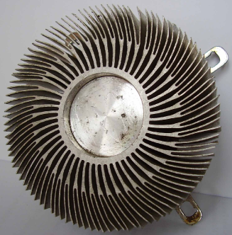
Figure 1: Heat radiator shaped like a thick fractal junction

Various constructions of thick junction type are successfully used in nanotechnologies [13], microtechnique [14], modern engineering constructions (microstrip radiator, ferrite-filled rod radiator), as well as many physical and biological systems. For example, a number of new applications are envisioned, especially regarding efficient sensors (inertial, biological, chemical), signal processing filters (ultra large band), micro-fractal constructions: fractal antennas, fractal transistors, fractal heat radiators and so on.

Such successful applications of thick-junction constructions have stimulated active learning BVP’s in thick junctions with more complex structures: thick junctions with the thin junction’s body [2, 3, 4], thick multi-level junctions [8, 9, 18], thick cascade junctions [5, 17], where new qualitative results were obtained. Specifically, it was shown that processes in thick multi-level junctions behave as a “many-phase system” and thick cascade junctions have new kind of eigenvibrations. This means that materials with such micro-structures have some new properties.

Designing such arrays of mechanical components in thick junctions cannot be achieved with today softwares, because this would require too much CPU resources. Regarding their number of components (in some cases few thousands), development of new mathematical tools are necessary. One of them is asymptotic analysis of BVP’s in thick junctions as $\varepsilon\to 0,$ i.e., when the number of attached thin domains infinitely increases and their thickness decreases to zero. Asymptotic results give us the possibility to replace the original problem in a thick junction by the corresponding homogenized problem that is more simpler and then apply computer simulation. In addition, in some cases it is possible to construct accurate and numerically implementable asymptotic approximations.

As a first step, here we consider a nonlinear boundary-value problem for a reaction-diffusion equation in a model $2D$ thick fractal junction $\Omega_{\varepsilon}$ (see Fig 2). Of course, it is possible to consider a thick fractal junction that has more complex branching structures. However, the main features in the asymptotic behavior of solutions to BVP’s in thick fractal junctions can be observed on the example of $\Omega_{\varepsilon}$ (a thick fractal junction with two branching levels).

The rest of this paper is organized as follows.

The statement of the problem and features of the investigation are given in Section 2.

In Section 3 we formally construct the leading terms of asymptotic expansions for a solution to our problem. The asymptotics consists of the outer expansions both in the junction’s body and in each thin branches as well as the leading terms of inner expansions in a neighborhood both of the joint zone and each branching levels.

Then in Section 4, using the method of matched asymptotic expansions, we derive the corresponding nonstandard homogenized problem. The existence and uniqueness of its solution in an anizotropic Sobolev space of multi-sheeted functions is proved in Section 5.

In Section 6 we construct an approximating function, find its residuals, estimate them and prove the main asymptotic estimate for the difference between the solution and the approximating function.

2 Statement of the problem

Let $\Omega_{0}$ be a bounded domain in $\mathbb{R}^{2}$ with the Lipschitz boundary $\partial\Omega_{0}$ and $\Omega_{0}\subset\{x:=(x_{1},x_{2})\in\mathbb{R}^{2}:\ x_{2}>0\}.$ Let $\partial\Omega_{0}$ contain the segment $I_{0}=\{x:x_{1}\in[0,a],\ \ x_{2}=0\}.$ We also assume that there exists a positive number $\delta_{0}$ such that $\Omega_{0}\cap\{x:\ 0<x_{2}<\delta_{0}\}=\{x:\ x_{1}\in(0,a),\ x_{2}\in(0,\delta_{0})\}.$

Let $a,l_{1},l_{2},l_{3}$ be positive numbers, $h_{0},h_{1,1},h_{1,2},h_{2,1},h_{2,2},h_{2,3},h_{2,4}$ be fixed numbers from the interval $(0,1)$ and $h_{1,1}+h_{1,2}<h_{0},$ $h_{2,1}+h_{2,2}<h_{1,1},$ $h_{2,3}+h_{2,4}<h_{1,2}.$ Let us also introduce a small parameter $\varepsilon=\frac{a}{N},$ where $N$ is a large positive integer.

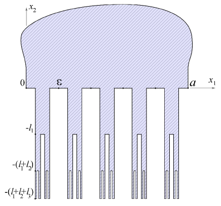
Figure 2: A model thick fractal junction $\Omega_{\varepsilon}$

A model thick fractal junction $\Omega_{\varepsilon}$ (see Fig. 2) consists of the junction’s body $\Omega_{0},$

• a large number of the thin rods $G^{(0)}_{\varepsilon}=\bigcup_{j=1}^{N-1}G^{(0)}_{j}(\varepsilon),$

  $$G^{(0)}_{j}(\varepsilon)=\left\{x:\,\left|x_{1}-\varepsilon(j+\frac{1}{2})\right|<\frac{\varepsilon h_{0}}{2},\quad x_{2}\in(-l_{1},0]\right\},$$

  from the zero layer,

• a large number of the thin rods $G^{(1,m)}_{\varepsilon}=\bigcup_{j=1}^{N-1}G^{(1,m)}_{j}(\varepsilon),$

  $$G^{(1,m)}_{j}(\varepsilon)=\left\{x:\,\left|x_{1}-\varepsilon(j+b_{1,m})\right|<\frac{\varepsilon h_{1,m}}{2},\quad x_{2}\in\big{(}-l_{2}-l_{1},-l_{1}\big{]}\right\},$$

  from the first branching layer, where $m\in\{1,2\}$ and

  $$b_{1,1}=\frac{1-h_{0}+h_{1,1}}{2},\quad b_{1,2}=\frac{1+h_{0}-h_{1,2}}{2},$$ (2.1)

• and a large number of the thin rods $G^{(2,m)}_{\varepsilon}=\bigcup_{j=1}^{N-1}G^{(2,m)}_{j}(\varepsilon),$

  $$G^{(2,m)}_{j}(\varepsilon)=\left\{x:\,\left|x_{1}-\varepsilon(j+b_{2,m})\right|<\frac{\varepsilon h_{2,m}}{2},\ \ x_{2}\in\big{(}-l_{3}-l_{2}-l_{1},-l_{2}-l_{1}\big{]}\right\},$$

from the second branching layer, where $m\in\{1,2,3,4\}$ and

$$b_{2,1}=\frac{1-h_{0}+h_{2,1}}{2},\quad b_{2,2}=\frac{1-h_{0}+2h_{1,1}-h_{2,2}}{2},$$ (2.2)

$$b_{2,3}=\frac{1+h_{0}-2h_{1,2}+h_{2,3}}{2},\quad b_{2,4}=\frac{1+h_{0}-h_{2,4}}{2}.$$ (2.3)

Thus, $\Omega_{\varepsilon}=\Omega_{0}\bigcup G^{(0)}_{\varepsilon}\bigcup G^{(1)}_{\varepsilon}\bigcup G^{(2)}_{\varepsilon},$ where $G^{(1)}_{\varepsilon}=\bigcup_{m=1}^{2}G^{(1,m)}_{\varepsilon},$ $G^{(2)}_{\varepsilon}=\bigcup_{m=1}^{4}G^{(2,m)}_{\varepsilon}.$ The small parameter $\varepsilon$ characterizes the distance between neighboring thin branches and also their thickness. Precisely, each branch $G^{(i,m)}_{j}(\varepsilon)$ has small cross-section of size ${\cal O}(\varepsilon)$ and constant height. In addition, at fixed $j\in\{0,1,\ldots,N-1\}$ branches $G^{(0)}_{j}(\varepsilon),$ $\{G^{(1,m)}_{j}(\varepsilon)\}_{m=1}^{2},$ $\{G^{(2,m)}_{j}(\varepsilon)\}_{m=1}^{4}$ form the tree with two branching levels. These trees are $\varepsilon$-periodically distributed along the segment $I_{0}.$

In $\Omega_{\varepsilon}$ we consider the following semilinear parabolic initial boundary-value problem:

$$\left\{\begin{array}[]{rcll}\partial_{t}v_{\varepsilon}-\Delta v_{\varepsilon}+k(v_{\varepsilon})&=&f_{0}&\mbox{in}\ \Omega_{0}\times(0,T),\\[5.69054pt] \partial_{t}v_{\varepsilon}-\Delta v_{\varepsilon}+k_{i}(v_{\varepsilon})&=&0&\mbox{in}\ G^{(i)}_{\varepsilon}\times(0,T),\quad i=0,1,2,\\[5.69054pt] \partial_{\nu}v_{\varepsilon}+\varepsilon^{\alpha_{i}}\kappa_{i}(v_{\varepsilon})&=&\varepsilon^{\beta_{i}}g^{(i)}_{\varepsilon}&\mbox{on}\ \Upsilon^{(i)}_{\varepsilon}\times(0,T),\quad i=0,1,2,\\[5.69054pt] \partial_{\nu}v_{\varepsilon}&=&0&\mbox{on}\ \partial\Omega_{\varepsilon}\setminus\Big{(}\bigcup_{i=0}^{2}\Upsilon^{(i)}_{\varepsilon}\Big{)}\times(0,T),\\[5.69054pt] \left[v_{\varepsilon}\right]_{\big{|}{x_{2}=-\sum_{n=0}^{i}l_{n}}}&=&\left[\partial_{x_{2}}v_{\varepsilon}\right]_{\big{|}{x_{2}=-\sum_{n=0}^{i}l_{n}}}=0&\mbox{on}\ Q^{(i)}_{\varepsilon}\times(0,T),\ \ i=0,1,2,\\[11.38109pt] \left.v_{\varepsilon}\right|_{t=0}&=&0&\mbox{in}\ \Omega_{\varepsilon},\end{array}\right.$$ (2.4)

where $\partial_{\nu}$ is the outward normal derivative; for each index $i\in\{0,1,2\}$ parameters $\alpha_{i}$ and $\beta_{i}$ are greater or equal $1,$ $\Upsilon^{(i)}_{\varepsilon}=\bigcup_{m=1}^{2i}\Upsilon^{(i,m)}_{\varepsilon},$ $\Upsilon^{(i,m)}_{\varepsilon}$ is the union of vertical boundaries of the thin rods $G^{(i,m)}_{\varepsilon},$ $Q^{(i)}_{\varepsilon}=G^{(i)}_{\varepsilon}\cap\{x_{2}=-\sum_{n=0}^{i}l_{n}\},$ $l_{0}=0,$ $f_{0},$ $g^{(i)}_{\varepsilon},$ $k,$ $k_{i},$ $\kappa_{i}$ are given functions;  the brackets denote the jump of the enclosed quantities.

Remark 2.1.

Hereafter we use the following shortening: $\{x_{2}=-\sum_{n=0}^{i}l_{n}\}:=\{x\in\mathbb{R}^{2}:\ x_{2}=-\sum_{n=0}^{i}l_{n}\};$ also if the index $i=0,$ then the index $m$ is absent and notation as $\Upsilon^{(0,m)}_{\varepsilon}$ means $\Upsilon^{(0)}_{\varepsilon}.$

Assumptions for the given functions are as follows. The function $f_{0}$ belongs to the space $L^{2}(\Omega_{0}\times(0,T))$ and its support is compactly embedded in $\Omega_{0}$ for a.e. $t\in(0,T).$ The functions $\{g^{(i)}_{\varepsilon}\}_{i=0}^{2}$ satisfy the following conditions:

• $g^{(i)}_{\varepsilon}\in L^{2}(D_{i}\times(0,T)),$ where the domain

  $$D_{i}=\Big{\{}x:\ 0<x_{1}<a,\ \ -\sum\nolimits_{n=0}^{i+1}l_{n}<x_{2}<-\sum\nolimits_{n=0}^{i}l_{n}\Big{\}}$$ (2.5)

  is filled up by the thin rods from the $i$-th layer in the limit passage as $\varepsilon\to 0;$

• there exist weak derivatives $\partial_{x_{1}}g^{(i)}_{\varepsilon}\in L^{2}(D_{i}\times(0,T)),\ i=0,1,2,$ and constants $c_{i},\,\varepsilon_{0}$ such that for each value $\varepsilon\in(0,\varepsilon_{0})$

  $$\|g^{(i)}_{\varepsilon}\|_{L^{2}(D_{i}\times(0,T))}\,+\,\|\partial_{x_{1}}g^{(i)}_{\varepsilon}\|_{L^{2}(D_{i}\times(0,T))}\,\leq\,c_{i};$$ (2.6)

• moreover, if $\ \beta_{i}=1,$ then there exists a function $g^{(i)}_{0}\in L^{2}(D_{i}\times(0,T))$ such that

  $$g^{(i)}_{\varepsilon}\to g^{(i)}_{0}\ \ \mbox{in}\ \ L^{2}(D_{i}\times(0,T))\quad\mbox{as}\ \ \varepsilon\to 0.$$ (2.7)

The functions $k:\mathbb{R}\to\mathbb{R},$ $k_{i}:\mathbb{R}\to\mathbb{R},$ and $\kappa_{i}:\mathbb{R}\to\mathbb{R},$ $i=0,1,2$ are continuously differentiable and

$$\exists\,c_{1},\,c_{2}>0:\ \ c_{1}\leq k^{\prime}\leq c_{2},\quad c_{1}\leq k^{\prime}_{i}\leq c_{2},\quad c_{1}\leq\kappa^{\prime}_{i}\leq c_{2}\ \ \ \text{ in}\ \mathbb{R},$$ (2.8)

$$i=0,1,2.$$

From (2.8) it follows (see e.g. [16]) the following inequalities:

$$c_{1}s^{2}+k(0)s\leq k(s)\,s\leq c_{2}s^{2}+k(0)s,$$ (2.9)

$$\exists\,c_{3}>0\ \ \forall\,p,\,s\in\mathbb{R}:\quad|k(p)-k(s)|\leq c_{3}|p-s|,\quad|k(s)|\leq c_{3}(1+|s|)$$ (2.10)

(the same inequalities for the other functions $\{k_{i}\},\{\kappa_{i}\}).$

Recall that a function $v_{\varepsilon}\in L^{2}\bigl{(}0,T;\,H^{1}(\Omega_{\varepsilon})\bigr{)},$ with $v^{\prime}_{\varepsilon}\in L^{2}\bigl{(}0,T;(H^{1}(\Omega_{\varepsilon}))^{*}\bigr{)},$ is a weak solution to problem (2.4) if

$$\langle v^{\prime}_{\varepsilon},\psi\rangle_{\varepsilon}+\langle{\cal A}_{\varepsilon}(t)v_{\varepsilon},\psi\rangle_{\varepsilon}=\langle F_{\varepsilon}(t),\psi\rangle_{\varepsilon}$$ (2.11)

for each $\psi\in H^{1}(\Omega_{\varepsilon})$ and a.e. $t\in(0,T),$ and $v_{\varepsilon}|_{t=0}=0.$

Here $\partial_{t}v_{\varepsilon}:=v^{\prime}_{\varepsilon},$ the brackets $\langle\cdot,\cdot\rangle_{\varepsilon}$ denotes the pairing of $H^{1}(\Omega_{\varepsilon})^{*}$ with $H^{1}(\Omega_{\varepsilon}),$ the operator ${\cal A}_{\varepsilon}(t):H^{1}(\Omega_{\varepsilon})\mapsto H^{1}(\Omega_{\varepsilon})^{*}$ is defined by the formula

$$\langle{\cal A}_{\varepsilon}(t)v,\psi\rangle_{\varepsilon}:=\int\limits_{\Omega_{\varepsilon}}\nabla_{x}v\cdot\nabla_{x}\psi\,dx+\int\limits_{\Omega_{0}}k(v)\,\psi\,dx+\sum_{i=0}^{2}\int\limits_{G^{(i)}_{\varepsilon}}k_{i}(v)\,\psi\,dx+\varepsilon^{\alpha_{i}}\int\limits_{\Upsilon_{\varepsilon}^{(i)}}\kappa_{i}(v)\,\psi\,dx_{2}$$

for all $v,\psi\in H^{1}(\Omega_{\varepsilon}),$ and the linear functional $F_{\varepsilon}(t)\in H^{1}(\Omega_{\varepsilon})^{*}$ is defined as follows:

$$\langle F_{\varepsilon}(t),\psi\rangle_{\varepsilon}:=\int\limits_{\Omega_{0}}f_{0}\,\psi\,dx+\sum_{i=0}^{2}\varepsilon^{\beta_{i}}\int\limits_{\Upsilon_{\varepsilon}^{(i)}}g^{(i)}_{\varepsilon}\,\psi\,dx_{2},\qquad\forall\psi\in H^{1}(\Omega_{\varepsilon}),$$

for a.e. $t\in[0,T].$ In addition, it is known that $v_{\varepsilon}\in C([0,T];L^{2}(\Omega_{\varepsilon}))$ and thus the equality $v_{\varepsilon}|_{t=0}=0$ makes sense.

Due to properties of the functions $k,k_{i},\kappa_{i},\ i=0,1,2,$ (see (2.8)-(2.10)) the operator ${\cal A}_{\varepsilon}$ is bounded, strictly monotone, hemicontinuous, and coercive (we verify these properties in more detail for the corresponding homogenized operator in Section 5). Then, from well-known results of the theory of monotone operators (see e.g. [23]) it follows that for each fixed value $\varepsilon>0$ there exists a unique weak solution to problem (2.4).

Our main research efforts are oriented towards the analytical understanding and asymptotic approximation of phenomena and processes in physics and biology which take place in thick fractal junctions involving, as models, nonlinear boundary-value problem (2.4). In particular, we want to find the corresponding homogenized problem as $\varepsilon\to 0,$ to construct the asymptotic approximation for the solution $v_{\varepsilon}$ and to study the influence of the parameters $\{\alpha_{i}\}$ and $\{\beta_{i}\}$ on the asymptotic behavior of the solution.

2.1 Features of the investigation

1. Thick junctions have special character of the connectedness: there are points in a thick junction, which are at a short distance of order ${\cal O}(\varepsilon),$ but the length of all curves, which connect these points in the junction, is order ${\cal O}(1).$ As a result, there are no extension operators that would be bounded uniformly in the corresponding Sobolev spaces [15]. At the same time the availability of an uniformly bounded family of extension operators is typical supposition in overwhelming majority of the existing homogenization schemes for problems in perforated domains with the Neumann or Robin boundary conditions (see e.g. [6, 7]). In addition, thick junctions are non-convex domains with non-smooth boundaries. Therefore, solutions of boundary-value problems in such domains have only minimal $H^{1}$-smoothness, while (see e.g. [7]) the $H^{2}$-smoothness of a solution is necessary to prove the convergence theorem. All these factors create special difficulties in the asymptotic analysis of BVP’s in thick junctions.

2. In a typical interpretation the solution to problem (2.4) denotes the density of some quantity (chemical concentration, temperature, electronic potential, etc) at equilibrium within the thick fractal junction $\Omega_{\varepsilon}.$ Usually for applied problems, the source of the quantity is located in the junction’s body. Therefore, the right-hand side $f_{0}$ is defined in $\Omega_{0}.$

3. Standard assumptions for nonlinear terms of reaction-diffusion equations are as follows: they are Lipschtz continuous functions. This hypothesis in particular implies $|k(s)|\leq C(1+|s|)$ for each $s\in\mathbb{R}$ and some constant $C.$ This is enough to state that problem (2.4) has a unique solution. But, if we want to construct some approximation for a solution and to prove the corresponding estimate, we need some kind of a coercivity condition on the nonlinearity. Usually it reads as follows: $k(s)s\geq C_{1}|s|^{2}-C_{2}$ for all $s\in\mathbb{R}$ and appropriate constants $C_{1}>0,$ $C_{2}\geq 0.$

   Many physical processes, especially in chemistry and medicine, have monotonous nature. Therefore, it is naturally to impose special monotonous conditions on the nonlinear terms. In our case we propose simple conditions (2.8) that imply the coercivity conditions (2.9).

4. Asymptotic behaviour of solutions to the reaction-diffusion equation in different kind of thin domains with the uniform Neumann conditions was studied in [1, 22]. The convergence theorems were proved under the following assumptions for the nonlinear term:
   in [1] it is a $C^{2}$-function with bounded derivatives and

   $$\limsup_{|s|\to+\infty}\frac{k(s)}{s}<0;$$ (2.12)

   in [22] it is a $C^{1}$-function, the dissipative condition (2.12) holds and

   $$|k^{\prime}(s)|\leq C(1+|s|^{q-1}),$$ (2.13)

   where $q\in(1,+\infty)$.

   Let us note that the convergence theorem for the solution to our problem (2.4) can be proved under more weak assumptions for the functions $k,\{k_{i}\},\{\kappa_{i}\},$ namely they are vanish at zero and satisfy inequality (2.13).

5. The nonlinear Robin boundary conditions are considered on the boundaries of the thin branches. These conditions mean that there is a flux of a quantity through the surfaces of the branches. In fact very small activity holds always on the surface of some material (therefore the Robin boundary conditions are more natural for applied mathematical problems). Such semilinear boundary conditions arise in many applied problems, in particular, in the modeling of chemical reactive flows. For instance, the following function

   $$\kappa(v)=\frac{\lambda\,v}{1+\mu\,v}\quad\text{with}\quad\lambda,\mu>0,$$

   which satisfies condition (2.8) if $f_{0}\geq 0$ and $g_{\varepsilon}^{(i)}\equiv 0,$ corresponds to the Michaelis-Menten hypothesis in biochemical reactions and to the Langmuir kinetics adsorption models (see [21, 7]).

6. In the interpretation mentioned above, the problem (2.4) describes the motion of a reactive fluid having different chemical features on different branching layers $(i=0,1,2)$ of the thick fractal junction. To study the influence of the boundary interactions on the asymptotic behavior of the solution, we introduce special intensity factors $\varepsilon^{\alpha_{i}}$ and $\varepsilon^{\beta_{i}}$ in the Robin boundary conditions on the lateral sides of the thin rectangles from the $i$-th branching layers.

   The effective behavior of this reactive flow (as $\varepsilon\to 0)$ is described by a new nonstandard homogenized parabolic problem containing extra zero-order terms which catch the effect of the chemical reactions depending on $\alpha_{i}$ and $\beta_{i}.$ The asymptotic behavior of the solution is described in Theorem 6.1. Here we note only that the following differential equations

   $$h_{i,m}\partial_{t}v^{(i,m)}_{0}-h_{i,m}\partial^{2}_{x_{2}x_{2}}v^{(i,m)}_{0}+h_{i,m}k_{i}\big{(}v^{(i,m)}_{0}\big{)}+2\delta_{\alpha_{i},1}\kappa_{i}\big{(}v^{(i,m)}_{0}\big{)}=2\delta_{\beta_{i},1}g^{(i)}_{0},\quad m=\overline{1,\,2i},$$

   form the homogenized relations in $D_{i}\times(0,T)$, where $\delta_{\alpha_{i},1},\delta_{\beta_{i},1}$ are Kronecker’s symbols.

7. It should be stressed that the important problem for each new proposed asymptotic method is its accuracy. Therefore, the proof of the error estimate for discrepancy between the constructed approximation and the exact solution is general principle that has been applied to the analysis of the efficiency of the proposed asymptotic method. With the help of special branch-layer solutions and the method of matched asymptotic expansions, the approximation for the solution is constructed and the corresponding asymptotic error estimate in the space $C\big{(}[0,T];L^{2}(\Omega_{\varepsilon})\big{)}\cap L^{2}\big{(}0,T;H^{1}(\Omega_{\varepsilon})\big{)}$ is proved in Theorem 6.1. From this theorem it follows directly the following corollary.

   Corollary 2.1.

   Let assumptions from Theorem 6.1 hold. Then for any $\rho\in(0,1)$

   $$\max_{t\in[0,T]}\Big{(}\|v_{\varepsilon}(\cdot,t)-v^{+}_{0}(\cdot,t)\|_{L^{2}(\Omega_{0})}+\sum_{i=0}^{2}\sum_{m=1}^{2i}\|v_{\varepsilon}(\cdot,t)-v^{(i,m)}_{0}(\cdot,t)\|_{L^{2}(G^{(i,m)}_{\varepsilon})}\Big{)}\\ \leq C_{0}\Big{(}\varepsilon^{1-\rho}+\sum_{i=0}^{2}\left(\varepsilon^{\alpha_{i}-1+\delta_{\alpha_{i},1}}+(1-\delta_{\beta_{i},1})\varepsilon^{\beta_{i}-1}+\delta_{\beta_{i},1}\|g^{(i)}_{\varepsilon}-g^{(i)}_{0}\|_{L^{2}(G^{(i)}_{\varepsilon})}\right)\Big{)},$$

   where $v_{\varepsilon}$ is the solution to problem (2.4), $\Big{(}v^{+},v^{(0)},\big{\{}v^{(1,m)}\big{\}}_{m=1}^{2},\,\big{\{}v^{(2,m)}\big{\}}_{m=1}^{4}\Big{)}$ is the multi-sheeted solution to the homogenized problem (5.1).

3 Formal asymptotic expansions for the solution

3.1 Outer expansions

Combining the algorithm of constructing asymptotics in thin domains with the methods of homogenization theory, we seek the main terms of the asymptotics for the solution $v_{\varepsilon}$ in the form

$$v_{\varepsilon}(x,t)\approx v^{+}_{0}(x,t)+\sum_{n=1}^{+\infty}\varepsilon^{n}v^{+}_{n}(x,t)\quad\mbox{in domain}\ \Omega_{0}\times(0,T)$$ (3.1)

and

$$v_{\varepsilon}(x,t)\approx v^{(i,m)}_{0}(x,t)+\sum_{n=1}^{+\infty}\varepsilon^{n}v^{(i,m)}_{n}(x,\tfrac{x_{1}}{\varepsilon}-j,t)$$ (3.2)

in the thin rod $G_{j}^{(i,m)}(\varepsilon)\times(0,T)$ from the $i$-th level, $j=0,\ldots,N-1.$ Let us recall that $i\in\{0,1,2\}$ and the index $m\in\{1,2\}$ for $i=1,$   $m\in\{1,2,3,4\}$ for $i=2,$ and if $i=0,$ then $m$ is absent and $G_{j}^{(0,m)}(\varepsilon)=G_{j}^{(0)}(\varepsilon)$ and $v^{(0,m)}_{n}=v^{(0)}_{n}.$

The asymptotic series (3.1) and (3.2) are usually called outer expansions.

Substituting the series (3.1) in the first equation of problem (2.4) and in the boundary conditions on $\partial\Omega_{0}\setminus I_{0},$ collecting coefficients of the same powers of $\varepsilon$ and taking into account the first estimate in (2.10), we get the following relations for the coefficient $v^{+}_{0}:$

$$\begin{array}[]{rcll}\partial_{t}v^{+}_{0}-\Delta v^{+}_{0}+k(v^{+}_{0})&=&f_{0}&\quad\text{in}\ \Omega_{0}\times(0,T),\\[2.84526pt] \partial_{\nu}v^{+}_{0}&=&0&\quad\text{on}\ \big{(}\partial\Omega_{0}\setminus I_{0}\big{)}\times(0,T).\end{array}$$ (3.3)

Now let us find limit relations in each domain $D_{i}$ (see (2.5)). Assuming for the moment that the functions $\{v^{(i,m)}_{n}\}$ in (3.2) are smooth, we write their Taylor series with respect to the variable $x_{1}$ at the point $x_{1}=\varepsilon(j+b_{i,m})$ (points $\{b_{i,m}\}$ are defined in (2.1)–(2.3), $b_{0,m}=b_{0}=\frac{1}{2}$) and pass to the ”fast”  variable $\xi_{1}=\varepsilon^{-1}x_{1};$   the indexes $i,$ $m$ and $j$ are fixed. Then (3.2) takes the form

$$v_{\varepsilon}(x,t)\approx v^{(i,m)}_{0}\bigl{(}\varepsilon(j+b_{i,m}),x_{2},t\bigr{)}+\sum_{n=1}^{+\infty}\varepsilon^{n}\,V^{(i,m,j)}_{n}(\xi_{1},x_{2},t),$$ (3.4)

where

$$V^{(i,m,j)}_{n}(\xi_{1},x_{2},t)=v^{(i,m)}_{n}\bigl{(}\varepsilon(j+b_{i,m}),x_{2},\xi_{1}-j,t\bigr{)}\\ +\sum_{p=1}^{n}{(\xi_{1}-j-b_{i,m})^{p}\over p!}\,{\partial^{p}v^{(i,m)}_{n-p}\over\partial x_{1}^{p}}\bigl{(}\varepsilon(j+b_{i,m}),x_{2},\xi_{1}-j,t\bigr{)}.$$ (3.5)

Let us substitute (3.4) into (2.4) instead of $v_{\varepsilon}.$ Since the Laplace operator takes the form $\Delta=\varepsilon^{-2}{\partial^{2}\over\partial\xi_{1}^{2}}+{\partial^{2}\over\partial x_{2}^{2}},$ the collection of coefficients of the same power of $\varepsilon$ gives us one dimensional boundary value problems with respect to $\xi_{1}$ for each $t\in(0,T).$ The first problem is the following:

$$\begin{array}[]{rcll}\partial^{2}_{\xi_{1}\xi_{1}}V^{(i,m,j)}_{1}(\xi_{1},x_{2},t)&=&0,&\quad\xi_{1}\in I_{h_{i,m}}(b_{i,m}),\\[2.84526pt] \partial_{\xi_{1}}V^{(i,m,j)}_{1}(b_{i,m}\pm\tfrac{h_{i,m}}{2},x_{2},t)&=&0,&\end{array}$$ (3.6)

where $\partial_{\xi_{1}}=\frac{\partial}{\partial\xi_{1}},$ $\partial^{2}_{\xi_{1}\xi_{1}}=\frac{\partial^{2}}{\partial\xi^{2}_{1}}$ and $I_{h_{i,m}}(b_{i,m})=\bigl{(}b_{i,m}-\frac{h_{i,m}}{2}\,,b_{i,m}+\frac{h_{i,m}}{2}\bigr{)};$  the variable $x_{2}$ is regarded as a parameter in this problem.

From (3.6) it follows that function $V^{(i,m,j)}_{1}$ doesn’t depend on $\xi_{1}.$ Therefore, $V^{(i,m,j)}_{1}$ is equal to some function $\varphi^{(i,m)}\bigl{(}\varepsilon(j+b_{i,m}),x_{2},t\bigr{)}.$ Since we look only for the first terms of the asymptotics, we can regard that $\varphi^{(i,m)}\equiv 0.$ Then, due to (3.5), we have

$$v^{(i,m)}_{1}\bigl{(}\varepsilon(j+b_{i,m}),x_{2},\xi_{1}-j,t\bigr{)}=-\bigl{(}\xi_{1}-j-b_{i,m}\bigr{)}\,\partial_{x_{1}}v^{(i,m)}_{0}\bigl{(}\varepsilon(j+b_{i,m}),x_{2},t\bigr{)}\,.$$ (3.7)

The problem for the function $V^{(i,m,j)}_{2}$ is as follows:

$$-\partial^{2}_{\xi_{1}\xi_{1}}V^{(i,m,j)}_{2}=\Big{(}\partial^{2}_{x_{2}x_{2}}v^{(i,m)}_{0}-k_{i}\big{(}v^{(i,m)}_{0}\big{)}-\partial_{t}v^{(i,m)}_{0}\Big{)}\Big{|}_{x_{1}=\varepsilon(j+b_{i,m})},\ \ \xi_{1}\in I_{h_{i,m}}(b_{i,m}),$$ (3.8)

$$\partial_{\xi_{1}}V^{(i,m,j)}_{2}\bigl{(}\xi_{1},x_{2},t\bigr{)}\big{|}_{\xi_{1}=b_{i,m}\pm\tfrac{h_{i,m}}{2}}=\Big{(}\mp\delta_{\alpha_{i},1}\kappa_{i}\big{(}v^{(i,m)}_{0}(x,t)\big{)}\pm\delta_{\beta_{i},1}g^{(i)}_{0}\bigl{(}x,t\bigr{)}\Big{)}\Big{|}_{x_{1}=\varepsilon(j+b_{i,m})},$$ (3.9)

where $\delta_{\alpha_{i},1},\delta_{\beta_{i},1}$ are Kronecker’s symbols (recall that $\alpha_{i}\geq 1$ and $\beta_{i}\geq 1).$

The solvability condition for problem (3.8)-(3.9) is given by the differential equation

$$h_{i,m}\partial_{t}v^{(i,m)}_{0}=h_{i,m}\partial^{2}_{x_{2}x_{2}}v^{(i,m)}_{0}-h_{i,m}k_{i}\big{(}v^{(i,m)}_{0}\big{)}-2\delta_{\alpha_{i},1}\kappa_{i}\big{(}v^{(i,m)}_{0}\big{)}+2\delta_{\beta_{i},1}g^{(i)}_{0}$$ (3.10)

with respect to variables $x_{2}$ and $t$ at the fixed value of $x_{1}=\varepsilon(j+b_{i,m}).$

Since the points $\{x_{1}=\varepsilon(j+b_{i,m}):\ j=0,\ldots,N-1\}$ form the $\varepsilon$-net in the interval $(0,a),$ we can extend all equations obtained above on $N$ segments to the rectangle $D_{i}$ $(i=0,1,2).$ Thus, we get the following differential equation

$$h_{0}\partial_{t}v^{(0)}_{0}=h_{0}\partial^{2}_{x_{2}x_{2}}v^{(0)}_{0}-h_{0}k_{0}\big{(}v^{(0)}_{0}\big{)}-2\delta_{\alpha_{0},1}\kappa_{0}\big{(}v^{(0)}_{0}\big{)}+2\delta_{\beta_{0},1}g^{(0)}_{0}$$ (3.11)

in $D_{0}\times(0,T)$ $(h_{0,m}=h_{0});$  we get two differential equations (m=1, 2)

$$h_{1,m}\partial_{t}v^{(1,m)}_{0}=h_{1,m}\partial^{2}_{x_{2}x_{2}}v^{(1,m)}_{0}-h_{1,m}k_{1}\big{(}v^{(1,m)}_{0}\big{)}-2\delta_{\alpha_{1},1}\kappa_{1}\big{(}v^{(1,m)}_{0}\big{)}+2\delta_{\beta_{1},1}g^{(1)}_{0}$$ (3.12)

in $D_{1}\times(0,T);$  and we get four differential equations (m=1, 2, 3, 4)

$$h_{2,m}\partial_{t}v^{(2,m)}_{0}=h_{2,m}\partial^{2}_{x_{2}x_{2}}v^{(2,m)}_{0}-h_{2,m}k_{2}\big{(}v^{(2,m)}_{0}\big{)}-2\delta_{\alpha_{2},1}\kappa_{2}\big{(}v^{(2,m)}_{0}\big{)}+2\delta_{\beta_{2},1}g^{(2)}_{0}$$ (3.13)

in $D_{2}\times(0,T).$ Here the variable $x_{1}$ is regarded as a parameter.

If we substitute (3.4) for $i=2$ into the Neumann condition on the bases

$$Q^{(3)}_{\varepsilon}=\overline{\Omega}_{\varepsilon}\cap\{x:\ x_{2}=-(l_{1}+l_{2}+l_{3})\}$$

and taking again that the points $\{x_{1}=\varepsilon(j+b_{2,m}):\ j=0,\ldots,N-1\}$ form the $\varepsilon$-net in the interval $(0,a)$ in account, we obtain the following boundary conditions for functions $\{v^{(2,m)}_{0}\}:$

$$\partial_{x_{2}}v^{(2,m)}_{0}\bigl{(}x_{1},-(l_{1}+l_{2}+l_{3}),t\bigr{)}=0,\quad m=1,2,3,4.$$ (3.14)

To find transmission conditions on the joint zone $I_{0}$ and on each branching zones $I_{1}=\{x:\ x_{1}\in(0,a),\ x_{2}=-l_{1}\},$ $I_{2}=\{x:\ x_{1}\in(0,a),\ x_{2}=-(l_{1}+l_{2})\},$ we use the method of matched asymptotic expansions for the outer expansions (3.1), (3.2) and inner expansions in neighborhoods of $I_{0},I_{1}$ and $I_{2}.$

3.2 Construction of inner expansions

3.2.1 Inner expansion in a neighborhood of $I_{0}$

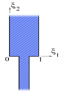
Figure 3: The cell of periodicity $\Pi_{0}$

In a neighborhood of the joint zone $I_{0}$ we introduce the ”rapid”  coordinates $\xi=(\xi_{1},\xi_{2}),$ where $\xi_{1}=\varepsilon^{-1}x_{1}$ and $\xi_{2}=\varepsilon^{-1}x_{2}.$ Passing to $\varepsilon=0,$ we see that the rod $G^{(0)}_{0}(\varepsilon)$ transforms into the semi-infinite strip

$$\Pi^{-}_{h_{0}}=\big{(}\frac{1}{2}-\frac{h_{0}}{2},\frac{1}{2}+\frac{h_{0}}{2}\big{)}\times(-\infty,0];$$

the domain $\Omega_{0}$ transforms into the first quadrant $\{\xi\,:\,\xi_{1}>0,\,\xi_{2}>0\}.$ Taking into account the periodic structure of $\Omega_{\varepsilon}$ in a neighborhood of $I_{0},$ we take the following cell of periodicity

$$\Pi_{0}=\Pi^{-}_{h_{0}}\cup\Pi^{+}$$

(see Fig. 3), where junction-layer problems will be considered; here $\Pi^{+}=(0,1)\times(0,+\infty).$ Obviously, solutions of these joint-layer problems must be 1-periodic in $\xi_{1},$ i.e.,

$$\partial^{p}_{\xi_{1}}Z(\xi)\arrowvert_{\xi_{1}=0}=\partial^{p}_{\xi_{1}}Z(\xi)\arrowvert_{\xi_{1}=1}\,,\qquad\xi\in\partial\Pi^{+}\,,\ \ \xi_{2}>0,\ \ \ \ p=0,1.$$ (3.15)

We propose the following ansatz for the inner asymptotic expansion in a neighborhood of $I_{0}\cap\Omega_{\varepsilon}:$

$$v_{\varepsilon}\approx v^{+}_{0}(x_{1},0,t)+\varepsilon\Bigl{(}Z^{(0)}_{1}\big{(}\tfrac{x}{\varepsilon}\big{)}\,\partial_{x_{1}}v^{+}_{0}(x_{1},0,t)+Z^{(0)}_{2}\big{(}\tfrac{x}{\varepsilon}\big{)}\,\partial_{x_{2}}v^{+}_{0}(x_{1},0,t)\Bigr{)}+\ldots$$ (3.16)

Substituting (3.16) in the differential equations of problem (2.4) and in the corresponding boundary conditions, taking into account that the Laplace operator takes the following form $\varepsilon^{-2}\Delta_{\xi}$ in the coordinates $\xi$ and collecting the coefficients of the same power of $\varepsilon,$ we arrive the following junction-layer problems for the coefficients $Z^{(0)}_{1}$ and $Z^{(0)}_{2}$ (to these problems we must add the periodic conditions (3.15)):

$$\begin{array}[]{rcll}-\Delta_{\xi}\ Z^{(0)}_{p}(\xi)&=&0,&\quad\xi\in\Pi_{0},\\ \partial_{\xi_{2}}Z^{(0)}_{p}(\xi_{1},0)&=&0,&\quad\xi_{1}\in(0,1)\setminus\big{(}\frac{1}{2}-\frac{h_{0}}{2},\frac{1}{2}-\frac{h_{0}}{2}\big{)},\\ \partial_{\xi_{1}}Z^{(0)}_{p}(\xi)&=&-\delta_{p,1},&\quad\xi\in\partial\Pi^{-}_{h_{1}}\cap\{\xi:\ \xi_{2}<0\},\qquad p=1,2.\end{array}$$ (3.17)

The existence and the main asymptotic relations for solutions of problems (3.17) can be obtained from general results about the asymptotic behavior of solutions to elliptic problems in domains with different exits to infinity [11, 20]. However, if a domain, where we consider a boundary-value problem, has some symmetry, then we can define more exactly the asymptotic relations and detect other properties of junction-layer solutions (see Lemma 4.1 and Corollary 4.1 from [15], see also [19]). From those results it follows the following proposition.

Proposition 3.1.

There exist unique solutions $Z^{(0)}_{1},Z^{(0)}_{2}\in H^{1}_{loc,\xi_{2}}(\Pi_{0})$ to problems (3.17) respectively, which have the following differentiable asymptotics

$$Z^{(0)}_{1}(\xi)=\begin{cases}\mathcal{O}(\exp(-2\pi\xi_{2})),&\xi_{2}\to+\infty,\\[8.53581pt] \displaystyle{\Big{(}\!-\xi_{1}+\frac{1}{2}\Big{)}}+\mathcal{O}(\exp(\pi h^{-1}_{0}\xi_{2})),&\xi_{2}\to-\infty,\end{cases}$$ (3.18)

$$Z^{(0)}_{2}(\xi)=\begin{cases}\xi_{2}+\mathcal{O}(\exp(-2\pi\xi_{2})),&\xi_{2}\to+\infty,\\[8.53581pt] \displaystyle{\frac{\xi_{2}}{h_{0}}}+C_{2}+\mathcal{O}(\exp(\pi h^{-1}_{0}\xi_{2})),&\xi_{2}\to-\infty,\end{cases}$$ (3.19)

Moreover, function $Z^{(0)}_{1}$ is odd in $\xi_{1}$ and function $Z^{(0)}_{2}$ is even in $\xi_{1}$ with respect to $\frac{1}{2}$.

Recall that a function $Z$ belongs to the Sobolev space $H^{1}_{loc,\xi_{2}}(\Pi_{0})$ if for every $R>0$ this function $Z\in H^{1}(\Pi_{0}\cap\{\xi:\,|\xi_{2}|<R\}).$

3.2.2 Inner expansion in a neighborhood of the first branching zone $I_{1}$

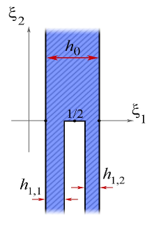
Figure 4: The cell of periodicity $\Pi_{0}$

In a neighborhood of $I_{1}$ we introduce the ”rapid”  coordinates $\xi=(\xi_{1},\xi_{2}),$ where $\xi_{1}=\varepsilon^{-1}x_{1}$ and $\xi_{2}=\varepsilon^{-1}(x_{2}+l_{1}).$ Passing to $\varepsilon=0$ , we see that the rod $G^{(0)}_{0}(\varepsilon)$ transforms into the semi-infinite strip

$$\Pi^{+}_{h_{0}}=\big{(}\frac{1}{2}-\frac{h_{0}}{2},\frac{1}{2}+\frac{h_{0}}{2}\big{)}\times(0,+\infty)$$

and rods $G^{(1,m)}_{0}(\varepsilon),\ m=1,2,$ transform into the semi-infinite strips

$$\Pi^{-}_{1,m}=\bigl{(}b_{1,m}-\frac{h_{1,m}}{2}\,,b_{1,m}+\frac{h_{1,m}}{2}\bigr{)}\times(-\infty,0],\ m=1,2,$$

respectively. Taking into account the periodic structure of $\Omega_{\varepsilon}$ in a neighborhood of $I_{1},$ we take the following cell of periodicity

$$\Pi_{1}=\Pi^{+}_{h_{0}}\cup\Pi^{-}_{1,1}\cup\Pi^{-}_{1,2},$$

where branch-layer problems will be considered.

Now we propose the following ansatz for the inner asymptotic expansion in a neighborhood of $I_{1}\cap\big{(}G^{(0)}_{\varepsilon}\cup G^{(1)}_{\varepsilon}\big{)}:$

$$v_{\varepsilon}(x,t)\approx v^{(0)}_{0}(x_{1},-l_{1},t)+\varepsilon\Bigl{(}Z^{(1)}_{1}\bigl{(}\tfrac{x_{1}}{\varepsilon},\tfrac{x_{2}+l_{1}}{\varepsilon}\bigr{)}\partial_{x_{1}}v^{(0)}_{0}(x_{1},-l_{1},t)\\ +\bigl{\{}\eta_{1}(x_{1},t)\,\Xi^{(1)}_{1}\big{(}\tfrac{x_{1}}{\varepsilon},\tfrac{x_{2}+l_{1}}{\varepsilon}\big{)}+(1-\eta_{1}(x_{1},t))\,\Xi^{(1)}_{2}\big{(}\tfrac{x_{1}}{\varepsilon},\tfrac{x_{2}+l_{1}}{\varepsilon}\big{)}\bigr{\}}\partial_{x_{2}}v^{(0)}_{0}(x_{1},-l_{1},t)\Bigr{)}+\ldots$$ (3.20)

where $Z^{(1)}_{1}(\xi),\,\Xi^{(1)}_{1}(\xi),\,\Xi^{(1)}_{2}(\xi),\ \xi\in\Pi_{1},$  are solutions to branch-layer problems, which 1-periodic extended along the coordinate axis $O_{\xi_{1}},$ the function $\eta_{1}$ will be defined from matching conditions.

Substituting (3.20) in the corresponding differential equation of problem (2.4) and boundary conditions, we arrive branch-layer problems for the functions $Z^{(1)}_{1},\,\Xi^{(1)}_{1},\,\Xi^{(1)}_{2}.$ So, the functions $\Xi^{(1)}_{1}$ and $\Xi^{(1)}_{2}$ are solution to the following homogeneous problem

$$\begin{array}[]{rcll}-\Delta_{\xi}\ \Xi(\xi)&=&0,&\quad\xi\in\Pi_{1},\\ \partial_{\xi_{1}}\Xi(\xi)&=&0,&\quad\xi\in\partial_{\parallel}\Pi_{1},\\ \partial_{\xi_{2}}\Xi(\xi_{1},0)&=&0,&\quad(\xi_{1},0)\in\partial\Pi_{1}\setminus\partial_{\parallel}\Pi_{1},\end{array}$$ (3.21)

where $\partial_{\parallel}\Pi_{1}$ is the union of the vertical sides of $\partial\Pi_{1}.$ Again using approach mentioned above, we conclude.

Proposition 3.2.

There exist two solutions $\Xi_{1},\,\Xi_{2}\in H^{1}_{loc,\xi_{2}}(\Pi_{1})$ to problems (3.21), which have the following differentiable asymptotics:

$$\Xi_{1}(\xi)=\left\{\begin{array}[]{ll}\xi_{2}+{\cal O}\big{(}\exp(-\frac{\pi\xi_{2}}{h_{0}})\big{)},&\ \ \xi_{2}\to+\infty,\ \xi\in\Pi^{+}_{h_{0}},\\[5.69054pt] \dfrac{h_{0}}{h_{1,1}}\,\xi_{2}+C_{1}^{(1)}+{\cal O}\big{(}\exp(\frac{\pi\xi_{2}}{h_{1,1}})\big{)},&\ \ \xi_{2}\to-\infty,\ \xi\in\Pi^{-}_{1,1},\\[11.38109pt] C_{2}^{(1)}+{\cal O}\big{(}\exp(\frac{\pi\xi_{2}}{h_{1,2}})\big{)},&\ \ \xi_{2}\to-\infty,\ \xi\in\Pi^{-}_{1,2},\end{array}\right.$$ (3.22)

$$\Xi_{2}(\xi)=\left\{\begin{array}[]{ll}\xi_{2}+{\cal O}\big{(}\exp(-\frac{\pi\xi_{2}}{h_{0}})\big{)},&\ \ \xi_{2}\to+\infty,\ \xi\in\Pi^{+}_{h_{0}},\\[5.69054pt] C_{1}^{(2)}+{\cal O}\big{(}\exp(\frac{\pi\xi_{2}}{h_{1,1}})\big{)},&\ \ \xi_{2}\to-\infty,\ \xi\in\Pi^{-}_{1,1},\\[5.69054pt] \dfrac{h_{0}}{h_{1,2}}\,\xi_{2}+C_{2}^{(2)}+{\cal O}\big{(}\exp(\frac{\pi\xi_{2}}{h_{1,2}})\big{)},&\ \ \xi_{2}\to-\infty,\ \xi\in\Pi^{-}_{1,2},\end{array}\right.$$ (3.23)

where $C_{1}^{(1)},C_{2}^{(1)},C_{1}^{(2)},C_{2}^{(2)}$ are some fixed constants.

Any another solution to the homogeneous problem (3.21), which has polynomial grow at infinity, can be presented as a linear combination $c_{0}+c_{1}\Xi_{1}+c_{2}\Xi_{2}.$

The function $Z^{(1)}_{1}$ is a solution to the following problem:

$$\begin{array}[]{rcll}-\Delta_{\xi}\ Z(\xi)&=&0,&\quad\xi\in\Pi_{1},\\ \partial_{\xi_{1}}Z(\xi)&=&-1,&\quad\xi\in\partial_{\parallel}\Pi_{1},\\ \partial_{\xi_{2}}Z(\xi_{1},0)&=&0,&\quad(\xi_{1},0)\in\partial\Pi_{1}\setminus\partial_{\parallel}\Pi_{1}.\end{array}$$ (3.24)

Proposition 3.3.

There exists the unique solution $Z\in H^{1}_{loc,\xi_{2}}(\Pi_{0})$ to problems (3.24), which has the following differentiable asymptotics:

$$Z(\xi)=\left\{\begin{array}[]{ll}-\xi_{1}+\frac{1}{2}+{\cal O}\big{(}\exp(-\frac{\pi\xi_{2}}{h_{0}})\big{)},&\ \ \xi_{2}\to+\infty,\ \xi\in\Pi^{+}_{h_{0}},\\ -\xi_{1}+b_{1,1}+C_{1}+{\cal O}\big{(}\exp(\frac{\pi\xi_{2}}{h_{1,1}})\big{)},&\ \ \xi_{2}\to-\infty,\ \xi\in\Pi^{-}_{1,1},\\[5.69054pt] -\xi_{1}+b_{1,2}+C_{2}+{\cal O}\big{(}\exp(\frac{\pi\xi_{2}}{h_{1,2}})\big{)},&\ \ \xi_{2}\to-\infty,\ \xi\in\Pi^{-}_{1,2},\end{array}\right.$$ (3.25)

where $C_{1},C_{2}$ are some fixed constants.

Thus, we set $\Xi^{(1)}_{1}=\Xi_{1},$ $\Xi^{(1)}_{2}=\Xi_{2}$ and $Z^{(1)}_{1}=Z.$

3.2.3 Inner expansion in a neighborhood of the second branching zone $I_{2}$

In a neighborhood of $I_{2}$ we introduce the ”rapid”  coordinates $\xi=(\xi_{1},\xi_{2}),$ where $\xi_{1}=\varepsilon^{-1}x_{1}$ and $\xi_{2}=\varepsilon^{-1}(x_{2}+l_{1}+l_{2}).$ Passing to $\varepsilon=0,$ we see that the rods $G^{(1,m)}_{0}(\varepsilon),\ m=1,2,$ transform into the semi-infinite strips $\Pi^{+}_{1,m}=\bigl{(}b_{1,m}-\frac{h_{1,m}}{2}\,,b_{1,m}+\frac{h_{1,m}}{2}\bigr{)}\times(0,+\infty),\ m=1,2,$ respectively, and the rods $G^{(2,m)}_{0}(\varepsilon),\ m=1,2,3,4,$ transform into the semi-infinite strips $\Pi^{-}_{2,m}=\bigl{(}b_{2,m}-\frac{h_{2,m}}{2}\,,b_{2,m}+\frac{h_{2,m}}{2}\bigr{)}\times(-\infty,0],\ m=1,2,3,4,$ respectively.

Taking into account the periodic structure of $\Omega_{\varepsilon}$ in a neighborhood of $I_{2},$ we take the following two cells of periodicity

$$\Pi^{(1)}_{2}=\Pi^{+}_{1,1}\cup\Pi^{-}_{2,1}\cup\Pi^{-}_{2,2}\quad\mbox{and}\quad\Pi^{(2)}_{2}=\Pi^{+}_{1,2}\cup\Pi^{-}_{2,3}\cup\Pi^{-}_{2,4},$$

where branch-layer problems will be considered.

Now we propose the following two inner asymptotic expansions in a neighborhood of $I_{2}\cap\big{(}G^{(1)}_{\varepsilon}\cup G^{(2)}_{\varepsilon}\big{)},$ namely the first one is as follows:

$$v_{\varepsilon}(x,t)\approx v^{(1,1)}_{0}(x_{1},0,t)+\varepsilon\Bigl{(}Z^{(2,1)}_{1}\bigl{(}\tfrac{x_{1}}{\varepsilon},\tfrac{x_{2}+l_{1}+l_{2}}{\varepsilon}\bigr{)}\,\partial_{x_{1}}v^{(1,1)}_{0}(x_{1},0,t)\\ +\Bigl{\{}\eta_{2,1}(x_{1},t)\,\Xi^{(2,1)}_{1}\big{(}\tfrac{x_{1}}{\varepsilon},\tfrac{x_{2}+l_{1}+l_{2}}{\varepsilon}\big{)}+(1-\eta_{2,1}(x_{1},t))\,\Xi^{(2,1)}_{2}\big{(}\tfrac{x_{1}}{\varepsilon},\tfrac{x_{2}+l_{1}+l_{2}}{\varepsilon}\big{)}\Bigr{\}}\partial_{x_{2}}v^{(1,1)}_{0}(x_{1},0,t)\Bigr{)}+\ldots$$ (3.26)

in a neighborhood of $I_{2}\cap\Big{(}G^{(1,1)}_{\varepsilon}\bigcup\big{(}\bigcup_{m=1}^{2}G^{(2,m)}_{\varepsilon}\big{)}\Big{)},$ and the second one

$$v_{\varepsilon}(x,t)\approx v^{(1,2)}_{0}(x_{1},0,t)+\varepsilon\Bigl{(}Z^{(2,2)}_{1}\bigl{(}\tfrac{x_{1}}{\varepsilon},\tfrac{x_{2}+l_{1}+l_{2}}{\varepsilon}\bigr{)}\,\partial_{x_{1}}v^{(1,2)}_{0}(x_{1},0,t)\\ +\Bigl{\{}\eta_{2,2}(x_{1},t)\,\Xi^{(2,2)}_{1}\big{(}\tfrac{x_{1}}{\varepsilon},\tfrac{x_{2}+l_{1}+l_{2}}{\varepsilon}\big{)}+(1-\eta_{2,2}(x_{1},t))\,\Xi^{(2,2)}_{2}\big{(}\tfrac{x_{1}}{\varepsilon},\tfrac{x_{2}+l_{1}+l_{2}}{\varepsilon}\big{)}\Bigr{\}}\partial_{x_{2}}v^{(1,2)}_{0}(x_{1},0,t)\Bigr{)}+\ldots$$ (3.27)

in a neighborhood of $I_{2}\cap\Big{(}G^{(1,2)}_{\varepsilon}\bigcup\big{(}\bigcup_{m=3}^{4}G^{(2,m)}_{\varepsilon}\big{)}\Big{)}.$

Coefficients $Z^{(2,1)}_{1}(\xi),\,\Xi^{(2,1)}_{1}(\xi),\,\Xi^{(2,1)}_{2}(\xi)\ \big{(}\xi\in\Pi^{(1)}_{2}\big{)}$ in (3.26) and coefficients $Z^{(2,2)}_{1}(\xi),$ $\Xi^{(2,2)}_{1}(\xi),$ $\Xi^{(2,2)}_{2}(\xi)\ \big{(}\xi\in\Pi^{(2)}_{2}\big{)}$ in (3.27) are solutions to branch-layer problems, which 1-periodic extended along the coordinate axis $O_{\xi_{1}};$ the functions $\eta_{2,1}$ and $\eta_{2,2}$ will be defined from matching conditions.

Namely, $Z^{(2,1)}_{1}$ and $Z^{(2,2)}_{1}$ are solutions to problem (3.24) but now in in $\Pi^{(1)}_{2}$ and $\Pi^{(2)}_{2}$ respectively. Applying results of Proposition 3.3, we can state that there exist the unique solutions with the following differentiable asymptotics:

$$Z^{(2,1)}_{1}(\xi)=\left\{\begin{array}[]{ll}-\xi_{1}+b_{1,1}+{\cal O}\big{(}\exp(-\frac{\pi\xi_{2}}{h_{1,1}})\big{)},&\ \ \xi_{2}\to+\infty,\ \xi\in\Pi^{+}_{1,1},\\ -\xi_{1}+b_{2,1}+C_{1}^{(3)}+{\cal O}\big{(}\exp(\frac{\pi\xi_{2}}{h_{2,1}})\big{)},&\ \ \xi_{2}\to-\infty,\ \xi\in\Pi^{-}_{2,1},\\[5.69054pt] -\xi_{1}+b_{2,2}+C_{2}^{(3)}+{\cal O}\big{(}\exp(\frac{\pi\xi_{2}}{h_{2,2}})\big{)},&\ \ \xi_{2}\to-\infty,\ \xi\in\Pi^{-}_{2,2},\end{array}\right.$$ (3.28)

$$Z^{(2,2)}_{1}(\xi)=\left\{\begin{array}[]{ll}-\xi_{1}+b_{1,2}+{\cal O}\big{(}\exp(-\frac{\pi\xi_{2}}{h_{1,2}})\big{)},&\ \ \xi_{2}\to+\infty,\ \xi\in\Pi^{+}_{1,2},\\ -\xi_{1}+b_{2,3}+C_{1}^{(4)}+{\cal O}\big{(}\exp(\frac{\pi\xi_{2}}{h_{2,3}})\big{)},&\ \ \xi_{2}\to-\infty,\ \xi\in\Pi^{-}_{2,3},\\[5.69054pt] -\xi_{1}+b_{2,4}+C_{2}^{(4)}+{\cal O}\big{(}\exp(\frac{\pi\xi_{2}}{h_{2,4}})\big{)},&\ \ \xi_{2}\to-\infty,\ \xi\in\Pi^{-}_{2,4}.\end{array}\right.$$ (3.29)

Functions $\Xi^{(2,1)}_{1},\Xi^{(2,1)}_{2}$ and $\Xi^{(2,2)}_{1},\Xi^{(2,2)}_{2}$ are solutions to problem (3.21) but now in $\Pi^{(1)}_{2}$ and $\Pi^{(2)}_{2}$ respectively. From Proposition 3.2 it follows that they have the corresponding differentiable asymptotics (3.22) and (3.23).

4 Matching of asymptotic expansions and homogenized problem

We have formally constructed the leading terms of the asymptotic expansions constructed in subsections 3.1 and 3.2 in different parts of the thick fractal junction $\Omega_{\varepsilon}.$ Next we apply the method of matched asymptotic expansions [10] to complete the constructions. Following this method, the asymptotics of the leading terms of outer expansions (3.1) and (3.2) as $x_{2}\to\pm-\sum_{p=0}^{m}l_{p},\ m=0,1,2,$ have to coincide with the corresponding asymptotics of the inner expansions (3.16), (3.20), (3.26) and (3.27) as $\eta_{2}\to\pm\infty$ respectively.

Near the point $(\varepsilon(j+\frac{1}{2}),0)\in I_{0}$ at the fixed value of $t,$ the function $v^{+}_{0}$ has the following asymptotics

$$v^{+}_{0}(\varepsilon(j+\tfrac{1}{2}),0,t)+\varepsilon\ \xi_{2}\,\partial_{x_{2}}v^{+}_{0}(\varepsilon(j+\tfrac{1}{2}),0,t)+\ldots\quad\text{as}\ x_{2}\to 0+0.$$

Taking into account the asymptotics of $Z^{(0)}_{1}$ and $Z^{(0)}_{2}$ as $\xi_{2}\to+\infty$ (see (3.18) and (3.19)), we conclude that the matching conditions are satisfied for the expansion (3.1) and (3.16).

The asymptotics of the outer expansion (3.2) is equal to

$$v^{(0)}_{0}(\varepsilon(j+\tfrac{1}{2}),0,t)+\varepsilon\Bigl{(}\bigl{(}-\xi_{1}+\tfrac{1}{2}+j\bigr{)}\,\partial_{x_{1}}v^{(0)}_{0}(\varepsilon(j+\tfrac{1}{2}),0,t)+\xi_{2}\,\partial_{x_{2}}v^{(0)}_{0}(\varepsilon(j+\tfrac{1}{2}),0,t)\Bigr{)}+\ldots$$ (4.1)

as $x_{2}\to 0-0,\quad(x,t)\in G^{(0)}_{j}(\varepsilon)\times(0,T).$ Keeping in mind the asymptotics of functions $Z^{(0)}_{1}$ and $Z^{(0)}_{2}$ as $\xi_{2}\to-\infty,$ we find the asymptotics of the leading terms of inner expansion (3.16)

$$v^{+}_{0}(\varepsilon(j+\tfrac{1}{2}),0,t)+\varepsilon\Bigl{(}\bigl{(}-\xi_{1}+j+\tfrac{1}{2}\bigr{)}\,\partial_{x_{1}}v^{+}_{0}(\varepsilon(j+\tfrac{1}{2}),0,t)+\bigl{(}\tfrac{\xi_{2}}{h_{0}}+C_{2}\bigr{)}\,\partial_{x_{2}}v^{+}_{0}(\varepsilon(j+\tfrac{1}{2}),0,t)\Bigr{)}+\ldots$$ (4.2)

as $\ \xi_{2}\to-\infty,\ \ \xi\in\Pi^{-}_{h_{0}}.$ Comparing terms of (4.1) and (4.2) at $\varepsilon^{0}$ and $\varepsilon$ respectively, we conclude that matching conditions are satisfied if

$$v^{+}_{0}(\varepsilon(j+\tfrac{1}{2}),0,t)=v^{(0)}_{0}(\varepsilon(j+\tfrac{1}{2}),0,t),\quad\partial_{x_{2}}v^{+}_{0}(\varepsilon(j+\tfrac{1}{2}),0,t)=h_{0}\partial_{x_{2}}v^{(0)}_{0}(\varepsilon(j+\tfrac{1}{2}),0,t),$$

$j=0,1,\ldots,N-1.$ Since the points $\{x_{1}=\varepsilon(j+\tfrac{1}{2}):\ j=0,\ldots,N-1\}$ form the $\varepsilon$-net in the interval $(0,a),$ we can spread these relations into all interval $I_{0}$ and get the first transmission conditions

$$v^{+}_{0}(x_{1},0,t)=v^{(0)}_{0}(x_{1},0,t),\quad(x_{1},t)\in(0,a)\times(0,T),$$ (4.3)

$$\partial_{x_{2}}v^{+}_{0}(x_{1},0,t)=h_{0}\,\partial_{x_{2}}v^{(0)}_{0}(x_{1},0,t),\quad(x_{1},t)\in(0,a)\times(0,T).$$ (4.4)

Now we verify matching conditions at the point $(\varepsilon(j+\frac{1}{2}),-l_{1})\in I_{1}.$ It is easy to see that they are satisfied for the expansion (3.2) as $x_{2}\to-l_{1}+0$ $(x\in G^{(0)}_{j}(\varepsilon))$ and for the expansion (3.20) as $\xi_{2}\to+\infty$ $(\xi\in\Pi^{+}_{h_{0}}).$

Bearing in mind (3.22), (3.23) and (3.25), we find at fixed value of $t\in(0,T)$ the following asymptotics of (3.20):

$$v^{(0)}_{0}(\varepsilon(j+b_{1,1}),-l_{1},t)\,+\,\varepsilon\Bigl{(}\bigl{(}-\xi_{1}+j+b_{1,1}+C_{1}\bigr{)}\,\partial_{x_{1}}v^{(0)}_{0}(\varepsilon(j+b_{1,1}),-l_{1},t)$$

$$+\Bigl{\{}\eta_{1}(\varepsilon(j+b_{1,1}),t)\,\bigl{(}\frac{h_{0}}{h_{1,1}}\,\xi_{2}+C^{(1)}_{1}\bigr{)}+\bigl{(}1-\eta_{1}(\varepsilon(j+b_{1,1},t))\bigr{)}C^{(2)}_{1}\Bigr{\}}\,\partial_{x_{2}}v^{(0)}_{0}(\varepsilon(j+b_{1,1}),-l_{1},t)\Bigr{)}+\ldots$$

$$\text{as}\ \ \xi_{2}\to-\infty,\ \ \xi\in\Pi^{-}_{1,1},$$ (4.5)

and

$$v^{(0)}_{0}(\varepsilon(j+b_{1,2}),-l_{1},t)\,+\,\varepsilon\Bigl{(}\bigl{(}-\xi_{1}+j+b_{1,2}+C_{2}\bigr{)}\,\partial_{x_{1}}v^{(0)}_{0}(\varepsilon(j+b_{1,2}),-l_{1},t)$$

$$+\Bigl{\{}\bigl{(}1-\eta_{1}(\varepsilon(j+b_{1,2},t))\bigr{)}\bigl{(}\frac{h_{0}}{h_{1,2}}\,\xi_{2}+C^{(2)}_{2}\bigr{)}+\eta_{1}(\varepsilon(j+b_{1,2}),t)\,C^{(1)}_{2}\Bigr{\}}\,\partial_{x_{2}}v^{(0)}_{0}(\varepsilon(j+b_{1,2}),-l_{1},t)\Bigr{)}+\ldots$$

$$\text{as}\ \ \xi_{2}\to-\infty,\ \ \xi\in\Pi^{-}_{1,2}.$$ (4.6)

Asymptotic forms of outer expansions (3.2) at $i=1$ and $m=1,2$ are equal to

$$v^{(1,1)}_{0}(\varepsilon(j+b_{1,1}),-l_{1},t)+\varepsilon\Bigl{(}\bigl{(}-\xi_{1}+b_{1,1}+j\bigr{)}\,\partial_{x_{1}}v^{(1,1)}_{0}(\varepsilon(j+b_{1,1}),-l_{1},t)$$

$$+\,\xi_{2}\,\partial_{x_{2}}v^{(1,1)}_{0}(\varepsilon(j+b_{1,1}),-l_{1},t)\Bigr{)}+\ldots$$ (4.7)

as $x_{2}\to-l_{1}-0,\ x\in G^{(1,1)}_{j}(\varepsilon),$ and

$$v^{(1,2)}_{0}(\varepsilon(j+b_{1,2}),-l_{1},t)+\varepsilon\Bigl{(}\bigl{(}-\xi_{1}+b_{1,2}+j\bigr{)}\,\partial_{x_{1}}v^{(1,2)}_{0}(\varepsilon(j+b_{1,2}),-l_{1},t)$$

$$+\xi_{2}\,\partial_{x_{2}}v^{(1,2)}_{0}(\varepsilon(j+b_{1,2}),-l_{1},t)\Bigr{)}+\ldots$$ (4.8)

as $x_{2}\to-l_{1}-0,\ x\in G^{(1,2)}_{j}(\varepsilon).$

To satisfy the matching conditions, we compare terms of (4.5) and (4.7), (4.6) and (4.8) at $\varepsilon^{0}$ and $\varepsilon^{1}.$ As a result, we get

$$v^{(0)}_{0}(\varepsilon(j+b_{1,m}),-l_{1},t)=v^{(1,m)}_{0}(\varepsilon(j+b_{1,m}),-l_{1},t),\quad m=1,2,$$

$$\eta_{1}(\varepsilon(j+b_{1,1}),t)\,h_{0}\,\partial_{x_{2}}v^{(0)}_{0}(\varepsilon(j+b_{1,1}),-l_{1},t)=h_{1,1}\,\partial_{x_{2}}v^{(1,1)}_{0}(\varepsilon(j+b_{1,1}),-l_{1},t),$$

$$\bigl{(}1-\eta_{1}(\varepsilon(j+b_{1,2},t))\bigr{)}\,h_{0}\,\partial_{x_{2}}v^{(0)}_{0}(\varepsilon(j+b_{1,2}),-l_{1},t)=h_{1,2}\,\partial_{x_{2}}v^{(1,2)}_{0}(\varepsilon(j+b_{1,2}),-l_{1},t),$$

for $j=0,1,\ldots,N-1.$ Since the sets $\{x_{1}=\varepsilon(j+b_{1,1}):\ j=0,\ldots,N-1\}$ $\{x_{1}=\varepsilon(j+b_{1,2}):\ j=0,\ldots,N-1\}$ form the $\varepsilon$-net in the interval $(0,a),$ we can spread these relations into all interval $I_{1}$ and deduce the second transmission conditions

$$v^{(0)}_{0}(x_{1},-l_{1},t)=v^{(1,m)}_{0}(x_{1},-l_{1},t),\quad m=1,2,$$ (4.9)

$$h_{0}\partial_{x_{2}}v^{(0)}_{0}(x_{1},-l_{1},t)=h_{1,1}\partial_{x_{2}}v^{(1,1)}_{0}(x_{1},-l_{1},t)+h_{1,2}\partial_{x_{2}}v^{(1,2)}_{0}(x_{1},-l_{1},t)$$ (4.10)

and determine the function

$$\eta_{1}(x_{1},t):=\frac{h_{1,1}\,\partial_{x_{2}}v^{(1,1)}_{0}(x_{1},-l_{1},t)}{h_{1,1}\,\partial_{x_{2}}v^{(1,1)}_{0}(x_{1},-l_{1},t)+h_{1,2}\,\partial_{x_{2}}v^{(1,2)}_{0}(x_{1},-l_{1},t)}$$ (4.11)

for $x_{1}\in(0,a)$ and $t\in(0,T).$

Due to (4.9)

$$\bigl{(}-\xi_{1}+j+b_{1,m}\bigr{)}\,\partial_{x_{1}}v^{(0)}_{0}(\varepsilon(j+b_{1,m}),-l_{1},t)=\bigl{(}-\xi_{1}+j+b_{1,m}\bigr{)}\,\partial_{x_{1}}v^{(1,m)}_{0}(\varepsilon(j+b_{1,m}),-l_{1},t),\quad m=1,2.$$

Therefore, the matching conditions are satisfied for the leading terms of asymptotic expansions (3.2) and (3.20) at each point $(\varepsilon(j+\frac{1}{2}),-l_{1})\in I_{1},$ $j=0,1,\ldots,N-1,$ if (4.9), (4.10) and (4.11) hold.

In analogous way we can deduce the following two kinds of transmission conditions at $x_{2}=-(l_{1}+l_{2}):$

$$v^{(1,1)}_{0}=v^{(2,1)}_{0}=v^{(2,2)}_{0}\quad\text{on}\ I_{2}\times(0,T),$$ (4.12)

$$h_{1,1}\partial_{x_{2}}v^{(1,1)}_{0}=h_{2,1}\partial_{x_{2}}v^{(2,1)}_{0}+h_{2,2}\partial_{x_{2}}v^{(2,2)}_{0}\quad\text{on}\ I_{2}\times(0,T),$$ (4.13)

and

$$v^{(1,2)}_{0}=v^{(2,3)}_{0}=v^{(2,4)}_{0}\quad\text{on}\ I_{2}\times(0,T),$$ (4.14)

$$h_{1,2}\partial_{x_{2}}v^{(1,2)}_{0}=h_{2,3}\partial_{x_{2}}v^{(2,3)}_{0}+h_{2,4}\partial_{x_{2}}v^{(2,4)}_{0}\quad\text{on}\ I_{2}\times(0,T).$$ (4.15)

In addition, the functions $\eta_{2,1}$ and $\eta_{2,2}$ in (3.26) and (3.27) are defined by formulas

$$\eta_{2,1}(x_{1},t)=\frac{h_{2,1}\,\partial_{x_{2}}v^{(2,1)}_{0}(x_{1},-(l_{1}+l_{2}),t)}{h_{2,1}\,\partial_{x_{2}}v^{(2,1)}_{0}(x_{1},-(l_{1}+l_{2}),t)+h_{2,2}\,\partial_{x_{2}}v^{(2,2)}_{0}(x_{1},-(l_{1}+l_{2}),t)},$$ (4.16)

$$\eta_{2,2}(x_{1},t)=\frac{h_{2,3}\,\partial_{x_{2}}v^{(2,3)}_{0}(x_{1},-(l_{1}+l_{2}),t)}{h_{2,3}\,\partial_{x_{2}}v^{(2,3)}_{0}(x_{1},-(l_{1}+l_{2}),t)+h_{2,4}\,\partial_{x_{2}}v^{(2,4)}_{0}(x_{1},-(l_{1}+l_{2}),t)}.$$ (4.17)

Relations (3.3), (3.11)-(3.14), (4.3), (4.4), (4.9), (4.10), (4.12)-(4.15) form homogenized problem for problem (2.4).

5 Operator formulation of the homogenized problem

To give appropriately the following definition of a weak solution of the homogenized problem, let us first introduce an anizotropic Sobolev space ${\bf H}$ of multi-sheeted functions. A multi-sheeted function

$$\boldsymbol{\varphi}:=\Big{(}\varphi^{+},\varphi^{(0)},\big{\{}\varphi^{(1,m)}\big{\}}_{m=1}^{2},\,\big{\{}\varphi^{(2,m)}\big{\}}_{m=1}^{4}\Big{)}=\left\{\begin{array}[]{ll}\varphi^{+}(x),&x\in\ \Omega_{0},\\ \varphi^{(0)}(x),&x\in\ D_{0},\\ \varphi^{(1,m)}(x),&x\in\ D_{1},\quad m=1,2,\\ \varphi^{(2,m)}(x),&x\in\ D_{2},\quad m=1,2,3,4,\end{array}\right.$$

belongs to ${\bf H}$ if $\varphi^{+}\in H^{1}(\Omega_{0}),$  $\{\varphi^{(i,m)}\}_{m=1}^{2i}\subset L^{2}(D_{i}),$ there exist weak derivatives $\{\partial_{x_{2}}\varphi^{(i,m)}\}_{m=1}^{2i}\subset L^{2}(D_{i}),\ i=0,1,2,$ and

$$\varphi^{+}|_{I_{0}}=\varphi^{(0)}|_{I_{0}},\qquad\varphi^{(0)}|_{I_{1}}=\varphi^{(1,1)}|_{I_{1}}=\varphi^{(1,2)}|_{I_{1}},$$

$$\varphi^{(1,1)}|_{I_{2}}=\varphi^{(2,1)}|_{I_{2}}=\varphi^{(2,2)}|_{I_{2}},\qquad\varphi^{(1,2)}|_{I_{2}}=\varphi^{(2,3)}|_{I_{2}}=\varphi^{(2,4)}|_{I_{2}}.$$

Obviously, the space ${\bf H}$ is continuously and densely embedded in the Hilbert space ${\bf V}$ of multi-sheeted functions whose components belong to the corresponding $L^{2}$-spaces, i.e., $\boldsymbol{\varphi}\in{\bf V}$ if $\varphi^{+}\in L^{2}(\Omega_{0}),$ $\{\varphi^{(i,m)}\}_{m=1}^{2i}\subset L^{2}(D_{i}),\ i=0,1,2.$ The scalar products in ${\bf V}$ and ${\bf H}$ are defined as follows:

$$\boldsymbol{(}\boldsymbol{\varphi},\boldsymbol{\psi}\boldsymbol{)}_{{\bf V}}:=(\varphi^{+},\psi^{+})_{L^{2}(\Omega_{0})}++\sum_{i=0}^{2}\sum_{m=1}^{2i}(\varphi^{(i,m)},\psi^{(i,m)})_{L^{2}(D_{i})},$$

$$\boldsymbol{(}\boldsymbol{\varphi},\boldsymbol{\psi}\boldsymbol{)}_{{\bf H}}:=\boldsymbol{(}\boldsymbol{\varphi},\boldsymbol{\psi}\boldsymbol{)}_{{\bf V}}+(\nabla\varphi^{+},\nabla\psi^{+})_{L^{2}(\Omega_{0})}+\sum_{i=0}^{2}\sum_{m=1}^{2i}(\partial_{x_{2}}\varphi^{(i,m)},\partial_{x_{2}}\psi^{(i,m)})_{L^{2}(D_{i})}$$

Recall that $\varphi^{(0,m)}=\varphi^{(0)}$ (see Remark 2.1). Since ${\bf H}$ is continuously and densely embedded in ${\bf V},$ we can construct the Gelfand triple ${\bf H}\subset{\bf V}\subset{\bf H}^{*}.$

For almost every $t\in[0,T]$ we introduce an operator $\boldsymbol{{\cal A}}(t):{\bf H}\mapsto{\bf H}^{*}$ by the formula

$$\boldsymbol{\langle}\boldsymbol{{\cal A}}(t)\boldsymbol{\varphi},\boldsymbol{\psi}\boldsymbol{\rangle}:=\int\limits_{\Omega_{0}}\Big{(}\nabla\varphi^{+}\cdot\nabla\psi^{+}+k(\varphi^{+})\psi^{+}\Big{)}\,dx$$

$$+\sum_{i=0}^{2}\sum_{m=1}^{2i}\int\limits_{D_{i}}\Big{(}h_{i,m}\partial_{x_{2}}\varphi^{(i,m)}\,\partial_{x_{2}}\psi^{(i,m)}+h_{i,m}k_{i}(\varphi^{(i,m)})\psi^{(i,m)}+2\delta_{\alpha_{i},1}\kappa_{i}(\varphi^{(i,m)})\psi^{(i,m)}\Big{)}dx$$

for all $\boldsymbol{\varphi},\boldsymbol{\psi}\in L^{2}(0,T;{\bf H}),$ and a linear functional ${\bf F}(t)\in{\bf H}^{*}$

$$\boldsymbol{\langle}{\bf F}(t),\boldsymbol{\psi}\boldsymbol{\rangle}:=\int\limits_{\Omega_{0}}f_{0}\psi^{+}\,dx+2\sum_{i=0}^{2}\delta_{\beta_{i},1}\sum_{m=1}^{2i}\int\limits_{D_{i}}g_{0}^{(i)}\psi^{(i,m)}dx.$$

Here $\boldsymbol{\langle\cdot,\cdot\rangle}$ is the pairing of ${\bf H}^{*}$ and ${\bf H},$  $\boldsymbol{\psi}=\Big{(}\psi^{+},\psi^{(0)},\big{\{}\psi^{(1,m)}\big{\}}_{m=1}^{2},\,\big{\{}\psi^{(2,m)}\big{\}}_{m=1}^{4}\Big{)}\in L^{2}(0,T;{\bf H}).$

Now we can write down the homogenized problem in the form of the abstract Cauchy problem

$${\bf v}^{\prime}+\boldsymbol{{\cal A}}({\bf v})={\bf F}\ \ \ \textrm{in}\ \ L^{2}\bigl{(}0,T;{\bf H}^{*}\bigr{)},\quad\ {\bf v}(0)=0,$$ (5.1)

where ${\bf v}=\Big{(}v^{+},v^{(0)},\big{\{}v^{(1,m)}\big{\}}_{m=1}^{2},\,\big{\{}v^{(2,m)}\big{\}}_{m=1}^{4}\Big{)}\in L^{2}(0,T;{\bf H}).$

Definition 5.1.

We say a multi-sheeted function

$${\bf v}\in L^{2}(0,T;{\bf H}),\quad\mbox{with}\quad{\bf v}^{\prime}\in L^{2}(0,T;{\bf H}^{*}),$$

is a weak solution to the homogenized problem provided

$$\boldsymbol{\langle}{\bf v}^{\prime}(t),{\bf u}\boldsymbol{\rangle}+\boldsymbol{\langle}\boldsymbol{{\cal A}}(t){\bf v},{\bf u}\boldsymbol{\rangle}=\boldsymbol{\langle}{\bf F}(t),{\bf u}\boldsymbol{\rangle}\quad\forall\ {\bf u}\in{\bf H}\ \ \mbox{and for a.e.}\ \ t\in(0,T),$$

and ${\bf v}|_{t=0}=0.$

Remark 5.1.

In view of the well-known properties of spaces $L^{p}(0,T;X)$ (see for instance [23]), the weak solution ${\bf v}\in C([0,T];{\bf V}),$ and thus the last equality in Definition 5.1 makes sence.

Theorem 5.1.

There exists a unique weak multi-sheeted solution to the homogenized problem.

Proof.

Let us show that for a.e. $t\in(0,T)$ the operator $\boldsymbol{{\cal A}}$ is bounded, strictly monotone, and hemicontinuous.

(1) Using (2.9), (6.17) and the definition of $\boldsymbol{{\cal A}},$ we can prove the following inequality

$$\big{|}\boldsymbol{\langle}\boldsymbol{{\cal A}}(t)\boldsymbol{\varphi},\boldsymbol{\psi}\boldsymbol{\rangle}\big{|}\leq C_{1}(1+\|\boldsymbol{\varphi}\|_{{\bf H}})\|\boldsymbol{\psi}\|_{{\bf H}}\quad\forall\,\boldsymbol{\varphi},\boldsymbol{\psi}\in{\bf H},$$

from where it follow that $\boldsymbol{{\cal A}}$ is bounded.

(2) Operator $\mathcal{A}$ is strongly monotone. Really, with the help of (2.8) we get

$$\boldsymbol{\langle}\boldsymbol{{\cal A}}\boldsymbol{\varphi}-\boldsymbol{{\cal A}}\boldsymbol{\psi},\boldsymbol{\varphi}-\boldsymbol{\psi}\boldsymbol{\rangle}\geq\int\limits_{\Omega_{0}}\Big{(}\big{|}\nabla(\varphi^{+}-\psi^{+})\big{|}^{2}+c_{1}\big{|}\varphi^{+}-\psi^{+}\big{|}^{2}\Big{)}\,dx$$

$$+\sum_{i=0}^{2}\sum_{m=1}^{2i}\int\limits_{D_{i}}\Big{(}h_{i,m}\big{|}\partial_{x_{2}}\varphi^{(i,m)}-\partial_{x_{2}}\psi^{(i,m)}\big{|}^{2}+(h_{i,m}+2\delta_{\alpha_{i},1})c_{1}\big{|}\varphi^{(i,m)}-\psi^{(i,m)}\big{|}^{2}\Big{)}\,dx$$

$$\geq C_{2}\|\boldsymbol{\varphi}-\boldsymbol{\psi}\|^{2}_{{\bf H}}\qquad\forall\ \boldsymbol{\varphi},\boldsymbol{\psi}\in{\bf H}.$$

(3) Operator $\boldsymbol{{\cal A}}$ is hemicontinuous. Indeed, the real valued function

$$[0,1]\ni\tau\longmapsto\boldsymbol{\langle}\boldsymbol{{\cal A}}(\boldsymbol{\varphi}+\tau\boldsymbol{\upsilon}),\boldsymbol{\psi}\boldsymbol{\rangle}$$

is continuous on $[0,1]$ for all fixed $\boldsymbol{\varphi},\boldsymbol{\psi},\boldsymbol{\upsilon}\in{\bf H}$ due to the continuity of the functions $\{k,k_{i},\kappa_{i}\},$ the right inequality in (2.10), and Lebesgue’s dominated convergence theorem.

Thus, the realization $\boldsymbol{{\cal A}}:L^{2}\bigl{(}0,T;{\bf H}\bigr{)}\mapsto L^{2}\bigl{(}0,T;{\bf H}^{*}\bigr{)}$ (we denote it by the same symbol) is bounded, monotone, and hemicontinuous, i.e., $\boldsymbol{{\cal A}}$ is type of $M$ (see Lemma 2.1 [23]).

(4) Operator $\mathcal{A}$ is coercive. Using (2.9), (2.10), and the Cauchy’s inequality with $\delta$ $(ab\leq\delta a^{2}+\frac{b^{2}}{4\delta},\ \ a,b,\delta>0),$ we find

$$\int_{0}^{T}\boldsymbol{\langle}\boldsymbol{{\cal A}}(t)\boldsymbol{\varphi},\boldsymbol{\varphi}\boldsymbol{\rangle}\,dt\geq C_{3}\int_{0}^{T}\|\boldsymbol{\varphi}\|^{2}_{{\bf H}}\,dt-|k(0)|\int\limits_{0}^{T}\int\limits_{\Omega_{0}}|\varphi^{+}|\,dxdt$$

$$-\sum_{i=0}^{2}\sum_{m=1}^{2i}\big{(}h_{i,m}|k_{i}(0)|+2\delta_{\alpha_{i},1}|\kappa_{i}(0)|\big{)}\int\limits_{0}^{T}\int\limits_{D_{i}}|\varphi^{(i,m)}|\,dxdt$$

$$\geq C_{3}\int_{0}^{T}\|\boldsymbol{\varphi}\|^{2}_{{\bf H}}\,dt-\delta\int_{0}^{T}\|\boldsymbol{\varphi}\|^{2}_{{\bf V}}\,dt-C_{4}(\delta)$$

for each $\boldsymbol{\varphi}\in L^{2}\bigl{(}0,T;{\bf H}\bigr{)}.$ By selecting appropriate $\delta,$ we obtain the desired inequality for the coerciveness.

By Corollary 4.1 [23], problem (5.1) has a unique solution. ∎

6 Asymptotic approximation

Let ${\bf v}=\Big{(}v^{+},v^{(0)},\big{\{}v^{(1,m)}\big{\}}_{m=1}^{2},\,\big{\{}v^{(2,m)}\big{\}}_{m=1}^{4}\Big{)}\in L^{2}(0,T;{\bf H})$ be a unique weak solution to the homogenized problem (5.1). With the help of ${\bf v},$ the junction-layer solutions $Z^{(0)}_{1}$ and $Z^{(0)}_{2}$ (see Proposition 3.1), the branch-layer solutions $\big{\{}Z^{(1)}_{1},\Xi^{(1)}_{1},\Xi^{(1)}_{2}\big{\}}$ (see Propositions 3.2, 3.3) in a neighborhood of the first branching zone $I_{1}$, and the branch-layer solutions $\big{\{}Z^{(2,1)}_{1},Z^{(2,2)}_{1},$ $\Xi^{(2,1)}_{1},\Xi^{(2,1)}_{2},\Xi^{(2,2)}_{1},\Xi^{(2,2)}_{2}\big{\}}$ in a neighborhood of the second branching zone $I_{2}$ (see § 3.2.3), we define the leading terms in the asymptotic expansions (3.1), (3.2), (3.16), (3.20), (3.26), and (3.27).

An approximating function $R_{\varepsilon}$ is constructed as the sum of the leading terms of the outer expansions (3.1), (3.2) and the inner expansion (3.16), (3.20), (3.26), (3.27) in neighborhoods of the joint zone $I_{0}$ and branching zones $I_{1},I_{2}$ respectively, with the subtraction of the identical terms of their asymptotics because they are summed twice. As a result, we obtain

$$R_{\varepsilon}(x,t)=v^{+}(x,t)+\varepsilon\chi_{0}(x_{2})\,{\cal N}^{(0)}_{+}\bigl{(}\tfrac{x}{\varepsilon},x_{1},t\bigr{)},\quad(x,t)\in\Omega_{0}\times(0,T);$$ (6.1)

$$R_{\varepsilon}=v^{(0)}(x,t)+\varepsilon\Bigl{(}Y_{0}(\tfrac{x_{1}}{\varepsilon})\,\partial_{x_{1}}v^{(0)}(x,t)+\chi_{0}(x_{2}){\cal N}^{(0)}_{-}\bigl{(}\tfrac{x}{\varepsilon},x_{1},t\bigr{)}+\chi_{1}(x_{2}){\cal N}^{(1)}\bigl{(}\tfrac{x_{1}}{\varepsilon},\tfrac{x_{2}+l_{1}}{\varepsilon},x_{1},t\bigr{)}\Bigr{)},\\ (x,t)\in G^{(0)}_{\varepsilon}\times(0,T);$$ (6.2)

$$R_{\varepsilon}=v^{(1,m)}(x,t)+\varepsilon\Bigl{(}Y_{1,m}(\tfrac{x_{1}}{\varepsilon})\,\partial_{x_{1}}v^{(1,m)}(x,t)+\chi_{1}(x_{2}){\cal N}^{(1)}_{1,m}\bigl{(}\tfrac{x_{1}}{\varepsilon},\tfrac{x_{2}+l_{1}}{\varepsilon},x_{1},t\bigr{)}$$

$$+\chi_{2}(x_{2}){\cal N}^{(2)}_{m}\bigl{(}\tfrac{x_{1}}{\varepsilon},\tfrac{x_{2}+l_{1}+l_{2}}{\varepsilon},x_{1},t\bigr{)}\Bigr{)},\quad(x,t)\in G^{(1,m)}_{\varepsilon}\times(0,T),\ m=1,2;$$ (6.3)

$$R_{\varepsilon}=v^{(2,m)}(x,t)+\varepsilon\Bigl{(}Y_{2,m}(\tfrac{x_{1}}{\varepsilon})\,\partial_{x_{1}}v^{(2,m)}(x,t)+\chi_{2}(x_{2}){\cal N}^{(2)}_{2,m}\bigl{(}\tfrac{x_{1}}{\varepsilon},\tfrac{x_{2}+l_{1}+l_{2}}{\varepsilon},x_{1},t\bigr{)}\Bigr{)},$$

$$(x,t)\in G^{(2,m)}_{\varepsilon}\times(0,T),\quad m=1,2,3,4.$$ (6.4)

Here the function $\chi_{0}$ is a smooth cutoff function such that $\chi_{0}(x_{2})=1$ for $|x_{2}|\leq\tau_{0}/2,$ and $\chi_{0}(x_{2})=0$ for $|x_{2}|\geq\tau_{0},$ where $\tau_{0}$ is sufficiently small number; $\chi_{1}(x_{2})=\chi_{0}(x_{2}+l_{1}),$ $\chi_{2}(x_{2})=\chi_{0}(x_{2}+l_{1}+l_{2}),$ $x_{2}\in\mathbb{R};$
in (6.1)

$${\cal N}^{(0)}_{+}\bigl{(}\xi,x_{1},t\bigr{)}=\sum_{i=1}^{2}\bigl{(}Z^{(0)}_{i}(\xi)-\delta_{i,2}\xi_{2}\bigr{)}\partial_{x_{i}}v^{+}(x_{1},0,t),\quad\xi=\tfrac{x}{\varepsilon},$$

where $\delta_{i,2}$ is the Kronecker delta;
in (6.2) $Y_{0}(\xi_{1})=-\xi_{1}+\frac{1}{2}+[\xi_{1}],$ where $[\xi_{1}]$ is the entire part of $\xi_{1},$ and

$${\cal N}^{(0)}_{-}=\Bigl{(}Z^{(0)}_{1}(\xi)-Y_{0}(\xi_{1})\Bigr{)}\partial_{x_{1}}v^{+}(x_{1},0,t)+\Big{(}Z^{(0)}_{2}(\xi)-\tfrac{\xi_{2}}{h_{0}}\Big{)}\partial_{x_{2}}v^{+}(x_{1},0,t),\quad\xi=\tfrac{x}{\varepsilon},$$

$${\cal N}^{(1)}=\Big{(}Z^{(1)}_{1}(\xi)-Y_{0}(\xi_{1})\Bigr{)}\partial_{x_{1}}v^{(0)}(x_{1},-l_{1},t)\\ +\Bigl{(}\eta_{1}(x_{1},t)\Xi^{(1)}_{1}(\xi)+(1-\eta_{1}(x_{1},t))\Xi^{(1)}_{2}(\xi)-\xi_{2}\Bigr{)}\partial_{x_{2}}v^{(0)}(x_{1},-l_{1},t),\\ \xi_{1}=\tfrac{x_{1}}{\varepsilon},\ \xi_{2}=\tfrac{x_{2}+l_{1}}{\varepsilon};$$

in (6.3) $Y_{1,m}(\xi_{1})=-\xi_{1}+b_{1,m}+[\xi_{1}],\ m=1,2,$ and

$${\cal N}^{(1)}_{1,m}\bigl{(}\xi,x_{1},t\bigr{)}=\Big{(}Z^{(1)}_{1}(\xi)-Y_{1,m}(\xi_{1})\Bigr{)}\partial_{x_{1}}v^{(0)}(x_{1},-l_{1},t)\\ +\Bigl{(}\eta_{1}(x_{1},t)\big{(}\Xi^{(1)}_{1}(\xi)-\delta_{1,m}\tfrac{h_{0}}{h_{1,1}}\xi_{2}\big{)}+(1-\eta_{1}(x_{1},t))\big{(}\Xi^{(1)}_{2}(\xi)-\delta_{2,m}\tfrac{h_{0}}{h_{1,2}}\xi_{2}\big{)}\Bigr{)}\partial_{x_{2}}v^{(0)}(x_{1},-l_{1},t),\\ \xi_{1}=\tfrac{x_{1}}{\varepsilon},\ \xi_{2}=\tfrac{x_{2}+l_{1}}{\varepsilon},$$

$${\cal N}^{(2)}_{m}\bigl{(}\xi,x_{1},t\bigr{)}=\Big{(}Z^{(2,m)}_{1}(\xi)-Y_{1,m}(\xi_{1})\Bigr{)}\partial_{x_{1}}v^{(1,m)}(x_{1},-l_{1}-l_{2},t)\\ +\Bigl{(}\eta_{2,m}(x_{1},t)\Xi^{(2,m)}_{1}(\xi)+(1-\eta_{2,m}(x_{1},t))\Xi^{(2,m)}_{2}(\xi)-\xi_{2}\Bigr{)}\partial_{x_{2}}v^{(1,m)}(x_{1},-l_{1}-l_{2},t),\\ \xi_{1}=\tfrac{x_{1}}{\varepsilon},\ \xi_{2}=\tfrac{x_{2}+l_{1}+l_{2}}{\varepsilon},\quad m=1,2;$$

in (6.4) $Y_{2,m}(\xi_{1})=-\xi_{1}+b_{2,m}+[\xi_{1}],\ m=1,2,3,4,$ and

$${\cal N}^{(2)}_{2,m}\bigl{(}\xi,x_{1},t\bigr{)}=\Big{(}Z^{(2,1)}_{1}(\xi)-Y_{2,m}(\xi_{1})\Bigr{)}\partial_{x_{1}}v^{(1,1)}(x_{1},-l_{1}-l_{2},t)\\ +\Bigl{(}\eta_{2,1}(x_{1},t)\big{(}\Xi^{(2,1)}_{1}(\xi)-\delta_{1,m}\tfrac{h_{1,1}}{h_{2,1}}\xi_{2}\big{)}+(1-\eta_{2,1}(x_{1},t))\big{(}\Xi^{(2,1)}_{2}(\xi)-\delta_{2,m}\tfrac{h_{1,1}}{h_{2,2}}\xi_{2}\big{)}\Bigr{)}\partial_{x_{2}}v^{(1,1)}(x_{1},-l_{1}-l_{2},t),\\ \xi_{1}=\tfrac{x_{1}}{\varepsilon},\ \xi_{2}=\tfrac{x_{2}+l_{1}+l_{2}}{\varepsilon},\ \ m=1,2,$$

$${\cal N}^{(2)}_{2,m}\bigl{(}\xi,x_{1},t\bigr{)}=\Big{(}Z^{(2,2)}_{1}(\xi)-Y_{2,m}(\xi_{1})\Bigr{)}\partial_{x_{1}}v^{(1,2)}(x_{1},-l_{1}-l_{2},t)\\ +\Bigl{(}\eta_{2,2}(x_{1},t)\big{(}\Xi^{(2,2)}_{1}(\xi)-\delta_{3,m}\tfrac{h_{1,2}}{h_{2,3}}\xi_{2}\big{)}+(1-\eta_{2,2}(x_{1},t))\big{(}\Xi^{(2,2)}_{2}(\xi)-\delta_{4,m}\tfrac{h_{1,2}}{h_{2,4}}\xi_{2}\big{)}\Bigr{)}\partial_{x_{2}}v^{(1,2)}(x_{1},-l_{1}-l_{2},t),\\ \xi_{1}=\tfrac{x_{1}}{\varepsilon},\ \xi_{2}=\tfrac{x_{2}+l_{1}+l_{2}}{\varepsilon},\ m=3,4.$$

Due to (4.3), (4.4), (4.9) and (4.12), the jumps $\left[R_{\varepsilon}\right]|_{Q^{(i)}_{\varepsilon}}=0,$ $i=0,1,2.$ This means that the approximating function $R_{\varepsilon}$ belongs to $L^{2}\bigl{(}0,T;\,H^{1}(\Omega_{\varepsilon})\bigr{)}.$

Theorem 6.1.

Suppose that in addition to the assumptions made in Section 2, the following conditions hold: the function $f_{0}\in C^{1}(\overline{\Omega_{0}}\times[0,T])$ and if some parameter $\beta_{i}=1$ $(i=0,1,2),$ then the function $g^{(i)}_{0}\in C^{1}(\overline{D_{i}}\times[0,T])$ and it and its derivative with respect to $x_{2}$ vanish at $x_{2}=-\sum_{n=0}^{i}l_{n}$ and $x_{2}=-\sum_{n=0}^{i+1}l_{n}.$

Then for any $\rho\in(0,1)$ there exist positive constants $C_{0},\varepsilon_{0}$ such that for all values $\varepsilon\in(0,\varepsilon_{0})$ the difference between the solution $v_{\varepsilon}$ to problem (2.4) and the approximating function $R_{\varepsilon}$ defined by (6.1) – (6.4) satisfies the following estimate

$$\max_{0\leq t\leq T}\|R_{\varepsilon}(\cdot,t)-v_{\varepsilon}(\cdot,t)\|_{L^{2}(\Omega_{\varepsilon})}+\|R_{\varepsilon}-v_{\varepsilon}\|_{L^{2}(0,T;H^{1}(\Omega_{\varepsilon}))}\\ \leq C_{0}\Big{(}\varepsilon^{1-\rho}+\sum_{i=0}^{2}\left(\varepsilon^{\alpha_{i}-1+\delta_{\alpha_{i},1}}+(1-\delta_{\beta_{i},1})\varepsilon^{\beta_{i}-1}+\delta_{\beta_{i},1}\|g^{(i)}_{\varepsilon}-g^{(i)}_{0}\|_{L^{2}(G^{(i)}_{\varepsilon})}\right)\Big{)}.$$ (6.5)

Proof.

I. Residuals in the differential equations.  Substituting $R_{\varepsilon}$ in the differential equations of problem (2.4) instead of $v_{\varepsilon}$ and calculating discrepancies with regard to problems (3.3), (3.11) – (3.13), we get

$$\partial_{t}R_{\varepsilon}-\Delta_{x}R_{\varepsilon}+k(R_{\varepsilon})-f_{0}=k(R_{\varepsilon})-k(v^{+})+\varepsilon\chi_{0}(x_{2})\partial_{t}{\cal N}_{+}^{(0)}(\xi,x_{1},t)|_{\xi=\frac{x}{\varepsilon}}\\ -\chi^{\prime}_{0}(x_{2})\bigl{(}\partial_{\xi_{2}}{\cal N}_{+}^{(0)}(\xi,x_{1},t)\bigr{)}\big{|}_{\xi=\frac{x}{\varepsilon}}-\varepsilon\partial_{x_{2}}\bigl{(}\chi^{\prime}_{0}(x_{2}){\cal N}_{+}^{(0)}(\tfrac{x}{\varepsilon},x_{1},t)\bigr{)}\\ -\chi_{0}(x_{2})\bigl{(}\partial^{2}_{x_{1}\xi_{1}}{\cal N}_{+}^{(0)}(\xi,x_{1},t)\bigr{)}\big{|}_{\xi=\frac{x}{\varepsilon}}-\varepsilon\chi_{0}(x_{2})\partial_{x_{1}}\big{(}\big{(}\partial_{x_{1}}{\cal N}_{+}^{(0)}(\xi,x_{1},t)\bigr{)}\big{|}_{\xi=\frac{x}{\varepsilon}}\big{)}\\ \text{in}\ \Omega_{0}\times(0,T);$$ (6.6)

$$\partial_{t}R_{\varepsilon}-\Delta_{x}R_{\varepsilon}+k_{0}(R_{\varepsilon})=k_{0}(R_{\varepsilon})-k_{0}(v^{(0)})-2\delta_{\alpha_{0},1}h^{-1}_{0}\kappa_{0}\big{(}v^{(0)}\big{)}+2\delta_{\beta_{0},1}h^{-1}_{0}g^{(0)}_{0}\\ -\varepsilon\partial_{x_{1}}\Bigl{(}Y_{0}(\tfrac{x_{1}}{\varepsilon})\partial^{2}_{x_{1}x_{1}}v^{(0)}\Bigr{)}-\varepsilon\partial_{x_{2}}\Bigl{(}Y_{0}(\tfrac{x_{1}}{\varepsilon})\partial^{2}_{x_{2}x_{1}}v^{(0)}\Bigr{)}\\ +\varepsilon\Bigl{(}Y_{0}(\tfrac{x_{1}}{\varepsilon})\,\partial^{2}_{tx_{1}}v^{(0)}(x,t)+\chi_{0}(x_{2})\partial_{t}{\cal N}^{(0)}_{-}\bigl{(}\tfrac{x}{\varepsilon},x_{1},t\bigr{)}+\chi_{1}(x_{2})\partial_{t}{\cal N}^{(1)}\bigl{(}\tfrac{x_{1}}{\varepsilon},\tfrac{x_{2}+l_{1}}{\varepsilon},x_{1},t\bigr{)}\Bigr{)}\\ -\chi^{\prime}_{0}(x_{2})\bigl{(}\partial_{\xi_{2}}{\cal N}^{(0)}_{-}(\xi,x_{1},t)\bigr{)}\big{|}_{\xi=\frac{x}{\varepsilon}}-\varepsilon\partial_{x_{2}}\bigl{(}\chi^{\prime}_{0}(x_{2}){\cal N}^{(0)}_{-}(\tfrac{x}{\varepsilon},x_{1},t)\bigr{)}\\ -\chi_{0}(x_{2})\bigl{(}\partial^{2}_{x_{1}\xi_{1}}{\cal N}^{(0)}_{-}(\xi,x_{1},t)\bigr{)}\big{|}_{\xi=\frac{x}{\varepsilon}}-\varepsilon\chi_{0}(x_{2})\partial_{x_{1}}\big{(}\big{(}\partial_{x_{1}}{\cal N}^{(0)}_{-}(\xi,x_{1},t)\bigr{)}\big{|}_{\xi=\frac{x}{\varepsilon}}\big{)}\\ -\chi^{\prime}_{1}(x_{2})\bigl{(}\partial_{\xi_{2}}{\cal N}^{(1)}(\xi,x_{1},t)\bigr{)}\big{|}_{\xi_{1}=\frac{x_{1}}{\varepsilon},\,\xi_{2}=\frac{x_{2}+l_{1}}{\varepsilon}}-\varepsilon\partial_{x_{2}}\bigl{(}\chi^{\prime}_{1}(x_{2}){\cal N}^{(1)}(\tfrac{x_{1}}{\varepsilon},\tfrac{x_{2}+l_{1}}{\varepsilon},x_{1},t)\bigr{)}\\ -\chi_{1}(x_{2})\bigl{(}\partial^{2}_{x_{1}\xi_{1}}{\cal N}^{(1)}(\xi,x_{1},t)\bigr{)}\big{|}_{\xi_{1}=\frac{x_{1}}{\varepsilon},\,\xi_{2}=\frac{x_{2}+l_{1}}{\varepsilon}}-\varepsilon\chi_{1}(x_{2})\partial_{x_{1}}\big{(}\big{(}\partial_{x_{1}}{\cal N}^{(1)}(\xi,x_{1},t)\bigr{)}\big{|}_{\xi_{1}=\frac{x_{1}}{\varepsilon},\,\xi_{2}=\frac{x_{2}+l_{1}}{\varepsilon}}\big{)}\\ \text{in}\ \ G^{(0)}_{\varepsilon}\times(0,T);$$ (6.7)

and similar relations in $G^{(1,m)}_{\varepsilon}\times(0,T),\ (m=1,2)$ and $G^{(2,m)}_{\varepsilon}\times(0,T),\ (m=1,2,3,4)$ up to replacement of indices.

II. Residuals in the boundary and initial conditions.  Obviously, $R_{\varepsilon}|_{t=0}=0.$ Also using (4.3), (4.4), (4.10), (4.11), (4.13), (4.15), (4.16) and (4.17), one can verify that

$$\left[\partial_{x_{2}}R_{\varepsilon}\right]\big{|}_{Q^{(0)}_{\varepsilon}}=-\varepsilon Y_{0}(\tfrac{x_{1}}{\varepsilon})\,\partial^{2}_{x_{1}x_{2}}v^{(0)}(x_{1},0,t),$$

$$\left[\partial_{x_{2}}R_{\varepsilon}\right]\big{|}_{Q^{(1,m)}_{\varepsilon}}=\varepsilon\Big{(}Y_{0}\partial^{2}_{x_{1}x_{2}}v^{(0)}(x,t)-Y_{1,m}\partial^{2}_{x_{1}x_{2}}v^{(1,m)}(x,t)\Big{)}|_{x_{2}=-l_{1}},\ m=1,2,$$

$$\left[\partial_{x_{2}}R_{\varepsilon}\right]\big{|}_{Q^{(2,m)}_{\varepsilon}}=\varepsilon\Big{(}Y_{1,1}\partial^{2}_{x_{1}x_{2}}v^{(1,1)}(x,t)-Y_{2,m}\partial^{2}_{x_{1}x_{2}}v^{(2,m)}(x,t)\Big{)}\big{|}_{x_{2}=-l_{1}-l_{2}},\ m=1,2,$$

$$\left[\partial_{x_{2}}R_{\varepsilon}\right]\big{|}_{Q^{(2,m)}_{\varepsilon}}=\varepsilon\Big{(}Y_{1,2}\partial^{2}_{x_{1}x_{2}}v^{(1,1)}(x,t)-Y_{2,m}\partial^{2}_{x_{1}x_{2}}v^{(2,m)}(x,t)\Big{)}|_{x_{2}=-l_{1}-l_{2}},\ m=3,4,$$ (6.8)

where $Q^{(i,m)}_{\varepsilon}=\partial G^{(i,m)}_{\varepsilon}\cap\{x_{2}=-\sum_{n=1}^{i}l_{n}\}.$

Since $Z^{(0)}_{1}$ is odd in $\xi_{1}$ and $Z^{(0)}_{2}$ is even in $\xi_{1}$ (see Proposition 3.1), it is easy to check that $\partial_{\nu}R_{\varepsilon}=0$ on $\partial\Omega_{\varepsilon}\cap\{x:x_{2}\geq 0\}.$ In additional, one can verify that

$$\partial_{x_{2}}R_{\varepsilon}\big{|}_{\partial\Omega_{\varepsilon}\cap\{x_{2}=-l_{1}\}}=\varepsilon\,Y_{0}(\tfrac{x_{1}}{\varepsilon})\,\partial^{2}_{x_{1}x_{2}}v^{(0)}(x_{1},-l_{1},t),$$

$$\partial_{x_{2}}R_{\varepsilon}\big{|}_{\partial\Omega_{\varepsilon}\cap\{x_{2}=-l_{1}-l_{2}\}\cap\partial G^{(1,m)}_{\varepsilon}}=\varepsilon\,Y_{1,m}(\tfrac{x_{1}}{\varepsilon})\,\partial^{2}_{x_{1}x_{2}}v^{(1,m)}(x_{1},-l_{1}-l_{2},t),\ m=1,2,$$

$$\partial_{x_{2}}R_{\varepsilon}|_{\partial\Omega_{\varepsilon}\cap\{x_{2}=-l_{1}-l_{2}-l_{3}\}}=0.$$ (6.9)

Taking into account boundary conditions in problems (3.17), (3.21), (3.24), we find the values of $\partial_{x_{1}}R_{\varepsilon}$ on the vertical boundary of the branches:

$$\partial_{x_{1}}R_{\varepsilon}=\varepsilon\Big{(}Y_{0}(\tfrac{x_{1}}{\varepsilon})\,\partial^{2}_{x_{1}x_{1}}v^{(0)}(x,t)+\chi_{0}(x_{2})\big{(}\partial_{x_{1}}{\cal N}^{(0)}_{-}(\xi,x_{1},t)\big{)}\big{|}_{\xi=\tfrac{x}{\varepsilon}}\\ +\chi_{1}(x_{2})\big{(}\partial_{x_{1}}{\cal N}^{(1)}(\xi,x_{1},t)\big{)}\big{|}_{\xi_{1}=\tfrac{x_{1}}{\varepsilon},\,\xi_{2}=\tfrac{x_{2}+l_{1}}{\varepsilon}}\Bigr{)}\quad\text{on}\ \partial G^{(0)}_{\varepsilon}\cap\{x_{2}\in(-l_{1},0)\},$$ (6.10)

$$\partial_{x_{1}}R_{\varepsilon}=\varepsilon\Big{(}Y_{1,m}(\tfrac{x_{1}}{\varepsilon})\,\partial^{2}_{x_{1}x_{1}}v^{(1,m)}(x,t)+\chi_{1}(x_{2})\big{(}\partial_{x_{1}}{\cal N}^{(1)}_{1,m}(\xi,x_{1},t)\big{)}\big{|}_{\xi_{1}=\tfrac{x_{1}}{\varepsilon},\,\xi_{2}=\tfrac{x_{2}+l_{1}}{\varepsilon}}\\ +\chi_{2}(x_{2})\big{(}\partial_{x_{1}}{\cal N}^{(2)}_{m}(\xi,x_{1},t)\big{)}\big{|}_{x_{1}=\tfrac{x_{1}}{\varepsilon},\,x_{2}=\tfrac{x_{2}+l_{1}+l_{2}}{\varepsilon}}\Bigr{)}\\ \text{on}\ \partial G^{(1,m)}_{\varepsilon}\cap\{x_{2}\in(-l_{1}-l_{2},-l_{1})\},\ \ m=1,2,$$ (6.11)

$$\partial_{x_{1}}R_{\varepsilon}=\varepsilon\Big{(}Y_{2,m}(\tfrac{x_{1}}{\varepsilon})\,\partial^{2}_{x_{1}x_{1}}v^{(2,m)}(x,t)+\chi_{2}(x_{2})\big{(}\partial_{x_{1}}{\cal N}^{(2)}_{2,m}(\xi,x_{1},t)\big{)}\big{|}_{x_{1}=\tfrac{x_{1}}{\varepsilon},\,x_{2}=\tfrac{x_{2}+l_{1}+l_{2}}{\varepsilon}}\Bigr{)}\\ \text{on}\ \partial G^{(2,m)}_{\varepsilon}\cap\{x_{2}\in(-l_{1}-l_{2}-l_{3},-l_{1}-l_{2})\},\ \ \quad m=1,2,3,4.$$ (6.12)

III. Residuals in the integral identity.  Multiplying (6.6) and (6.7) for each indexes $i$ and $m$ with arbitrary function $\psi\in L^{2}(0,T;H^{1}(\Omega_{\varepsilon})),$ integrating by parts and taking (6.8)–(6.12) into account, we deduce

$$\int\limits_{\Omega_{\varepsilon}}\partial_{t}R_{\varepsilon}\,\psi\,dx+\langle{\cal A}_{\varepsilon}(t)R_{\varepsilon},\psi\rangle_{\varepsilon}=\int\limits_{\Omega_{0}}f_{0}\,\psi\,dx+{\cal F}_{\varepsilon}(\psi)$$ (6.13)

for a.e. $t\in(0,T].$ Subtracting the integral identity (2.11) from (6.13) and integrating over $t\in(0,\tau),$ where $\tau\in(0,T],$ we get

$$\int_{0}^{\tau}\Big{(}\langle R^{\prime}_{\varepsilon}-v^{\prime}_{\varepsilon},\psi\rangle_{\varepsilon}+\langle{\cal A}_{\varepsilon}(t)R_{\varepsilon}-{\cal A}_{\varepsilon}(t)v_{\varepsilon},\psi\rangle_{\varepsilon}\Big{)}\,dt\\ =\int_{0}^{\tau}\Big{(}{\cal F}_{\varepsilon}(\psi)-\sum_{i=0}^{2}\varepsilon^{\beta_{i}}\int\limits_{\Upsilon_{\varepsilon}^{(i)}}g^{(i)}_{\varepsilon}\,\psi\,dx_{2}\Big{)}\,dt,$$ (6.14)

where ${\cal F}_{\varepsilon}(\psi)=\sum_{j=1}^{5}{\cal I}^{\varepsilon}_{j}(\psi)$ and (to short formulas we omit variables $\frac{x}{\varepsilon},x,t$ in some places)

$${\cal I}^{\varepsilon}_{1}(\psi)=\int\limits_{\Omega_{0}}\big{(}k(R_{\varepsilon})-k(v^{+})\big{)}\,\psi\,dx+\sum_{i=0}^{2}\sum_{m=1}^{2i}\int\limits_{G^{(i,m)}_{\varepsilon}}\big{(}k_{i}(R_{\varepsilon})-k_{i}(v^{(i,m)})\big{)}\,\psi\,dx,$$

$${\cal I}^{\varepsilon}_{2}(\psi)=\sum_{i=0}^{2}\sum_{m=1}^{2i}\Bigg{(}\varepsilon^{\alpha_{i}}\int\limits_{\Upsilon_{\varepsilon}^{(i,m)}}\kappa_{i}(R_{\varepsilon})\,\psi\,dx_{2}-2\delta_{\alpha_{i},1}h^{-1}_{i,m}\int\limits_{G^{(i,m)}_{\varepsilon}}\kappa_{i}\big{(}v^{(i,m)}\big{)}\,\psi\,dx\Bigg{)},$$

$${\cal I}^{\varepsilon}_{3}(\psi)=2\sum_{i=0}^{2}\sum_{m=1}^{2i}\delta_{\beta_{i},1}h^{-1}_{i,m}\int\limits_{G^{(i,m)}_{\varepsilon}}g^{(i)}_{0}\,\psi\,dx,$$

$${\cal I}^{\varepsilon}_{4}(\psi)=\varepsilon\Bigg{(}\int\limits_{\Omega_{0}}\Big{(}\chi_{0}(x_{2})\partial_{t}{\cal N}_{+}^{(0)}\,\psi+\chi^{\prime}_{0}(x_{2}){\cal N}_{+}^{(0)}\,\partial_{x_{2}}\psi+\chi_{0}(x_{2})\big{(}\partial_{x_{1}}{\cal N}_{+}^{(0)}(\xi,x_{1},t)\bigr{)}\big{|}_{\xi=\frac{x}{\varepsilon}}\,\partial_{x_{1}}\psi\Big{)}\,dx$$

$$+\sum_{i=0}^{2}\sum_{m=1}^{2i}\int\limits_{G^{(i,m)}_{\varepsilon}}Y_{i,m}(\tfrac{x_{1}}{\varepsilon})\big{(}\partial^{2}_{x_{2}x_{1}}v^{(i,m)}\,\partial_{x_{2}}\psi+\partial^{2}_{x_{1}x_{1}}v^{(i,m)}\,\partial_{x_{1}}\psi\big{)}\,dx$$

$$+\int\limits_{G^{(0)}_{\varepsilon}}\Bigl{(}Y_{0}(\tfrac{x_{1}}{\varepsilon})\,\partial^{2}_{tx_{1}}v^{(0)}+\chi_{0}(x_{2})\partial_{t}{\cal N}^{(0)}_{-}\bigl{(}\tfrac{x}{\varepsilon},x_{1},t\bigr{)}+\chi_{1}(x_{2})\partial_{t}{\cal N}^{(1)}\bigl{(}\tfrac{x_{1}}{\varepsilon},\tfrac{x_{2}+l_{1}}{\varepsilon},x_{1},t\bigr{)}\Bigr{)}\,\psi\,dx$$

$$+\int\limits_{G^{(0)}_{\varepsilon}}\Big{(}\chi_{0}(x_{2})\big{(}\partial_{x_{1}}{\cal N}^{(0)}_{-}(\xi,x_{1},t)\bigr{)}\big{|}_{\xi=\frac{x}{\varepsilon}}+\chi_{1}(x_{2})\big{(}\partial_{x_{1}}{\cal N}^{(1)}(\xi,x_{1},t)\bigr{)}\big{|}_{\xi_{1}=\frac{x_{1}}{\varepsilon},\,\xi_{2}=\frac{x_{2}+l_{1}}{\varepsilon}}\Big{)}\partial_{x_{1}}\psi\,dx$$

$$+\int\limits_{G^{(0)}_{\varepsilon}}\Big{(}\chi^{\prime}_{0}(x_{2}){\cal N}^{(0)}_{-}(\tfrac{x}{\varepsilon},x_{1},t)+\chi^{\prime}_{1}(x_{2}){\cal N}^{(1)}(\tfrac{x_{1}}{\varepsilon},\tfrac{x_{2}+l_{1}}{\varepsilon},x_{1},t)\Big{)}\partial_{x_{2}}\psi\,dx$$

$$+\sum_{m=1}^{2}\int\limits_{G^{(1,m)}_{\varepsilon}}\Bigl{(}Y_{1,m}(\tfrac{x_{1}}{\varepsilon})\,\partial^{2}_{tx_{1}}v^{(1,m)}+\chi_{1}\,\partial_{t}{\cal N}^{(1)}_{1,m}\bigl{(}\tfrac{x_{1}}{\varepsilon},\tfrac{x_{2}+l_{1}}{\varepsilon},x_{1},t\bigr{)}+\chi_{2}\,\partial_{t}{\cal N}^{(2)}_{m}\bigl{(}\tfrac{x_{1}}{\varepsilon},\tfrac{x_{2}+l_{1}+l_{2}}{\varepsilon},x_{1},t\bigr{)}\Bigr{)}\,\psi\,dx$$

$$+\int\limits_{G^{(1,m)}_{\varepsilon}}\Big{(}\chi_{1}\,\big{(}\partial_{x_{1}}{\cal N}^{(1)}_{1,m}(\xi,x_{1},t)\bigr{)}\big{|}_{\xi_{1}=\frac{x_{1}}{\varepsilon},\,\xi_{2}=\frac{x_{2}+l_{1}}{\varepsilon}}+\chi_{2}\,\big{(}\partial_{x_{1}}{\cal N}^{(2)}_{m}(\xi,x_{1},t)\bigr{)}\big{|}_{\xi_{1}=\frac{x_{1}}{\varepsilon},\,\xi_{2}=\frac{x_{2}+l_{1}+l_{2}}{\varepsilon}}\Big{)}\partial_{x_{1}}\psi\,dx$$

$$+\int\limits_{G^{(1,m)}_{\varepsilon}}\Big{(}\chi^{\prime}_{1}(x_{2}){\cal N}^{(1)}_{1,m}(\tfrac{x_{1}}{\varepsilon},\tfrac{x_{2}+l_{1}}{\varepsilon},x_{1},t)+\chi^{\prime}_{2}(x_{2}){\cal N}^{(2)}_{m}(\tfrac{x_{1}}{\varepsilon},\tfrac{x_{2}+l_{1}+l_{2}}{\varepsilon},x_{1},t)\Big{)}\partial_{x_{2}}\psi\,dx$$

$$+\sum_{m=1}^{4}\int\limits_{G^{(2,m)}_{\varepsilon}}\Bigl{(}Y_{2,m}(\tfrac{x_{1}}{\varepsilon})\,\partial^{2}_{tx_{1}}v^{(2,m)}+\chi_{2}(x_{2})\,\partial_{t}{\cal N}^{(2)}_{2,m}\bigl{(}\tfrac{x_{1}}{\varepsilon},\tfrac{x_{2}+l_{1}+l_{2}}{\varepsilon},x_{1},t\bigr{)}\Bigr{)}\,\psi\,dx$$

$$+\int\limits_{G^{(2,m)}_{\varepsilon}}\chi_{2}(x_{2})\,\big{(}\partial_{x_{1}}{\cal N}^{(2)}_{2,m}(\xi,x_{1},t)\bigr{)}\big{|}_{\xi_{1}=\frac{x_{1}}{\varepsilon},\,\xi_{2}=\frac{x_{2}+l_{1}+l_{2}}{\varepsilon}}\,\partial_{x_{1}}\psi\,dx$$

$$+\int\limits_{G^{(2,m)}_{\varepsilon}}\chi^{\prime}_{2}(x_{2}){\cal N}^{(2)}_{2,m}(\tfrac{x_{1}}{\varepsilon},\tfrac{x_{2}+l_{1}+l_{2}}{\varepsilon},x_{1},t)\,\partial_{x_{2}}\psi\,dx\Bigg{)},$$

$${\cal I}^{\varepsilon}_{5}(\psi)=-\int\limits_{\Omega_{0}}\chi^{\prime}_{0}(x_{2})\bigl{(}\partial_{\xi_{2}}{\cal N}_{+}^{(0)}(\xi,x_{1},t)\bigr{)}\big{|}_{\xi=\frac{x}{\varepsilon}}\,\psi\,dx$$

$$-\int\limits_{G^{(0)}_{\varepsilon}}\Big{(}\chi^{\prime}_{0}(x_{2})\bigl{(}\partial_{\xi_{2}}{\cal N}^{(0)}_{-}(\xi,x_{1},t)\bigr{)}\big{|}_{\xi=\frac{x}{\varepsilon}}+\chi^{\prime}_{1}(x_{2})\bigl{(}\partial_{\xi_{2}}{\cal N}^{(1)}(\xi,x_{1},t)\bigr{)}\big{|}_{\xi_{1}=\frac{x_{1}}{\varepsilon},\,\xi_{2}=\frac{x_{2}+l_{1}}{\varepsilon}}\Big{)}\psi\,dx$$

$$-\sum_{m=1}^{2}\int\limits_{G^{(1,m)}_{\varepsilon}}\Big{(}\chi^{\prime}_{1}\bigl{(}\partial_{\xi_{2}}{\cal N}^{(1)}_{1,m}(\xi,x_{1},t)\bigr{)}\big{|}_{\xi_{1}=\frac{x_{1}}{\varepsilon},\,\xi_{2}=\frac{x_{2}+l_{1}}{\varepsilon}}+\chi^{\prime}_{2}\bigl{(}\partial_{\xi_{2}}{\cal N}^{(2)}_{m}(\xi,x_{1},t)\bigr{)}\big{|}_{\xi_{1}=\frac{x_{1}}{\varepsilon},\,\xi_{2}=\frac{x_{2}+l_{1}+l_{2}}{\varepsilon}}\Big{)}\psi\,dx$$

$$-\sum_{m=1}^{4}\int\limits_{G^{(2,m)}_{\varepsilon}}\chi^{\prime}_{2}(x_{2})\,\bigl{(}\partial_{\xi_{2}}{\cal N}^{(2)}_{2,m}(\xi,x_{1},t)\bigr{)}\big{|}_{\xi_{1}=\frac{x_{1}}{\varepsilon},\,\xi_{2}=\frac{x_{2}+l_{1}+l_{2}}{\varepsilon}}\,\psi\,dx,$$

$${\cal I}^{\varepsilon}_{6}(\psi)=-\int\limits_{\Omega_{0}}\chi_{0}(x_{2})\bigl{(}\partial^{2}_{x_{1}\xi_{1}}{\cal N}_{+}^{(0)}(\xi,x_{1},t)\bigr{)}\big{|}_{\xi=\frac{x}{\varepsilon}}\psi\,dx$$

$$-\int\limits_{G^{(0)}_{\varepsilon}}\Big{(}\chi_{0}(x_{2})\bigl{(}\partial^{2}_{x_{1}\xi_{1}}{\cal N}^{(0)}_{-}(\xi,x_{1},t)\bigr{)}\big{|}_{\xi=\frac{x}{\varepsilon}}+\chi_{1}(x_{2})\bigl{(}\partial^{2}_{x_{1}\xi_{1}}{\cal N}^{(1)}(\xi,x_{1},t)\bigr{)}\big{|}_{\xi_{1}=\frac{x_{1}}{\varepsilon},\,\xi_{2}=\frac{x_{2}+l_{1}}{\varepsilon}}\Big{)}\psi\,dx$$

$$-\sum_{m=1}^{2}\int\limits_{G^{(1,m)}_{\varepsilon}}\Big{(}\chi_{1}\bigl{(}\partial^{2}_{x_{1}\xi_{1}}{\cal N}^{(1)}_{1,m}(\xi,x_{1},t)\bigr{)}\big{|}_{\xi_{1}=\frac{x_{1}}{\varepsilon},\,\xi_{2}=\frac{x_{2}+l_{1}}{\varepsilon}}+\chi_{2}\bigl{(}\partial^{2}_{x_{1}\xi_{1}}{\cal N}^{(2)}_{m}(\xi,x_{1},t)\bigr{)}\big{|}_{\xi_{1}=\frac{x_{1}}{\varepsilon},\,\xi_{2}=\frac{x_{2}+l_{1}+l_{2}}{\varepsilon}}\Big{)}\psi\,dx$$

$$-\sum_{m=1}^{4}\int\limits_{G^{(2,m)}_{\varepsilon}}\chi_{2}(x_{2})\,\bigl{(}\partial^{2}_{x_{1}\xi_{1}}{\cal N}^{(2)}_{2,m}(\xi,x_{1},t)\bigr{)}\big{|}_{\xi_{1}=\frac{x_{1}}{\varepsilon},\,\xi_{2}=\frac{x_{2}+l_{1}+l_{2}}{\varepsilon}}\,\psi\,dx.$$

Let us estimate the right-hand side in (6.14). Due to the conditions (2.8) we have $|{\cal I}^{\varepsilon}_{1}(\psi)|\leq C_{1}\varepsilon\|\psi\|_{L^{2}(\Omega_{\varepsilon})}.$ To estimate $|{\cal I}^{\varepsilon}_{2}(\psi)|,$ we use special integral identities

$$\frac{\varepsilon h_{i,m}}{2}\int\limits_{\Upsilon_{\varepsilon}^{(i,m)}}\phi\>dx_{2}=\int\limits_{G_{\varepsilon}^{(i,m)}}\phi\>dx-\varepsilon\int\limits_{G^{(i,m)}_{\varepsilon}}Y_{i,m}\left(\frac{x_{1}}{\varepsilon}\right)\partial_{x_{1}}\phi\>dx\quad\forall\>\phi\in H^{1}\bigl{(}G^{(i,m)}_{\varepsilon}\bigr{)},$$ (6.15)

for $i\in\{0,1,2\},\ m=\overline{1,2i}.$ To prove (6.15) it is enough to integrate by parts the last integral in (6.15). If $\alpha_{i}=1,$ then with the help of (6.15) we deduce

$$\Bigg{|}\varepsilon^{1}\int\limits_{\Upsilon_{\varepsilon}^{(i,m)}}\kappa_{i}(R_{\varepsilon})\,\psi\,dx_{2}-2h^{-1}_{i,m}\int\limits_{G^{(i,m)}_{\varepsilon}}\kappa_{i}\big{(}v^{(i,m)}\big{)}\,\psi\,dx\Bigg{|}\\ \leq 2h^{-1}_{i,m}\int\limits_{G^{(i,m)}_{\varepsilon}}\Big{|}\kappa_{i}(R_{\varepsilon})-\kappa_{i}\big{(}v^{(i,m)}\big{)}\Big{|}\big{|}\psi\big{|}\,dx\,+\,\varepsilon\int\limits_{G^{(i,m)}_{\varepsilon}}\Big{|}Y_{i,m}\left(\frac{x_{1}}{\varepsilon}\right)\Big{|}\big{|}\partial_{x_{1}}\big{(}\kappa_{i}(R_{\varepsilon})\psi\big{)}\big{|}\,dx\\ \leq C_{2}\varepsilon\|\psi\|_{H^{1}(\Omega_{\varepsilon})}.$$ (6.16)

In the last inequality we use (2.8), (6.17) and inequality $\max_{\mathbb{R}}|Y_{i,m}|\leq 1.$ If $\alpha_{i}>1,$ then again with the help of (6.15) we get

$$\Bigg{|}\varepsilon^{\alpha_{i}}\int_{\Upsilon_{\varepsilon}^{(i,m)}}\kappa_{i}(R_{\varepsilon})\,\psi\,dx_{2}\Bigg{|}\leq C_{3}\varepsilon^{\alpha_{i}-1}\|\psi\|_{H^{1}(\Omega_{\varepsilon})}.$$

Therefore, $|{\cal I}^{\varepsilon}_{2}(\psi)|\leq C_{4}\sum_{i=0}^{2}\varepsilon^{\alpha_{i}-1+\delta_{\alpha_{i},1}}\|\psi\|_{H^{1}(\Omega_{\varepsilon})}.$

Similar, but now using (2.6) and (2.7), we can estimate

$$\Bigg{|}{\cal I}^{\varepsilon}_{3}(\psi)-\sum_{i=0}^{2}\varepsilon^{\beta_{i}}\int\limits_{\Upsilon_{\varepsilon}^{(i)}}g^{(i)}_{\varepsilon}\,\psi\,dx_{2}\Bigg{|}\\ \leq C_{5}\|\psi\|_{H^{1}(\Omega_{\varepsilon})}\sum_{i=0}^{2}\Big{(}(1-\delta_{\beta_{i},1})\varepsilon^{\beta_{i}-1}+\delta_{\beta_{i},1}\big{(}\|g^{(i)}_{\varepsilon}-g^{(i)}_{0}\|_{L^{2}(G^{(i,m)}_{\varepsilon})}+\varepsilon\big{)}\Big{)}.$$

It is easy to see that ${\cal I}^{\varepsilon}_{4}(\psi)$ is of order ${\cal O}(\varepsilon).$ Thanks to the asymptotic estimates (3.18), (3.19), (3.22) – (3.25), all integrals in ${\cal I}^{\varepsilon}_{5}(\psi)$ are integrated over the support of the functions $\{\chi^{\prime}_{i}\}_{i=0}^{2}.$ Therefore, they are exponentially small.

Since the functions $\partial^{2}_{x_{1}\xi_{1}}{\cal N}_{+}^{(0)},$ $\partial^{2}_{x_{1}\xi_{1}}{\cal N}_{-}^{(0)},$ $\partial^{2}_{x_{1}\xi_{1}}{\cal N}^{(1)},$ $\{\partial^{2}_{x_{1}\xi_{1}}{\cal N}_{1,m}^{(1)},\partial^{2}_{x_{1}\xi_{1}}{\cal N}^{(2)}_{m}\}_{m=1}^{2},$ $\{\partial^{2}_{x_{1}\xi_{1}}{\cal N}_{2,m}^{(2)}\}_{m=1}^{4}$ exponentially decrease as $|\xi_{2}|\to+\infty$ (see (3.18), (3.19), (3.22) – (3.25)), we deduce from Lemma 3.1 ([19]) that for any $\rho\in(0,1)$ the integrals in ${\cal I}^{\varepsilon}_{6}(\psi)$ are of order ${\cal O}(\varepsilon^{1-\rho}).$

Regarding to the inequalities obtained above in this subsection, we conclude that for the right-hand side in (6.14) for every $\tau\in(0,T]$ the following inequality holds

$$\Bigg{|}\int\limits_{0}^{\tau}\Big{(}{\cal F}_{\varepsilon}(\psi)-\sum_{i=0}^{2}\varepsilon^{\beta_{i}}\int\limits_{\Upsilon_{\varepsilon}^{(i)}}g^{(i)}_{\varepsilon}\,\psi\,dx_{2}\Big{)}\,dt\Bigg{|}\leq C\|\psi\|_{L^{2}(0,T;H^{1}(\Omega_{\varepsilon}))}\,\\ \times\Big{(}\varepsilon^{1-\rho}+\sum_{i=0}^{2}\big{(}\varepsilon^{\alpha_{i}-1+\delta_{\alpha_{i},1}}+(1-\delta_{\beta_{i},1})\varepsilon^{\beta_{i}-1}+\delta_{\beta_{i},1}\|g^{(i)}_{\varepsilon}-g^{(i)}_{0}\|_{L^{2}(G^{(i)}_{\varepsilon})}\big{)}\Big{)}.$$ (6.17)

Putting $R_{\varepsilon}-v_{\varepsilon}$ instead $\psi$ in (6.13) and taking into account that ${\cal A}_{\varepsilon}$ is strictly monotone, we derive from (6.13) and (6.17) the estimate (6.5). ∎

Remark 6.1.

The constant $C_{0}$ in (6.5) depends on the following quantities:

$$\sup_{(x_{1},t)\in(0,a)\times(0,T)}\,\bigl{|}\partial^{2}_{tx_{j}}v^{+}(x_{1},0,t)\bigr{|},\quad\sup_{(x_{1},t)\in(0,a)\times(0,T)}\,\bigl{|}\mathcal{D}^{\alpha}v^{+}(x_{1},0,t)\bigr{|},$$

$$\sup_{(x_{1},t)\in(0,a)\times(0,T)}\,\bigl{|}\partial^{2}_{tx_{j}}v^{(0)}(x_{1},-l_{1},t)\bigr{|},\quad\sup_{(x_{1},t)\in(0,a)\times(0,T)}\,\bigl{|}\mathcal{D}^{\alpha}v^{(0)}(x_{1},-l_{1},t)\bigr{|},$$

$$\sup_{(x_{1},t)\in(0,a)\times(0,T)}\,\bigl{|}\partial^{2}_{tx_{j}}v^{(1,m)}(x_{1},-l_{1}-l_{2},t)\bigr{|},\ \sup_{(x_{1},t)\in(0,a)\times(0,T)}\,\bigl{|}\mathcal{D}^{\alpha}v^{(1,m)}(x_{1},-l_{1}-l_{2},t)\bigr{|},$$

$m=1,2,\ j=1,2,$ and $\|\partial^{2}_{tx_{1}}v^{(i,m)}_{0}\|_{L^{2}(D_{i}\times(0,T))},$ where $i\in\{0,1,2\},$ $m=\overline{1,2i},$ $\ |\alpha|=\alpha_{1}+\alpha_{2}\leq 2.$  Due to the assumptions for the functions $f_{0}$ and $\{g^{(i)}_{0}\}_{i=0}^{2}$ and condition (2.8) it follows from classical results on the smoothness of solutions to semilinear parabolic problems (see for instance §6 and §7 from [12, Sec. V]) that these quantities are bounded.

From Theorem 6.1 it follows directly the Corollary 2.1.

References

[1]
J.M. Arrieta, A.N. Carvalho, M.C. Pereira, R.P. Silva:
Semilinear parabolic problems in thin domains with a highly
oscillatory boundary. Nonlinear Analysis, 74 (2011) 5111–5132
[2]
D. Blanchard, A. Gaudiello: Homogenization of highly oscillating boundaries and reduction of dimention for monotone problem. ESAIM: COCV. 9 (2003) 449–460.
[3]
D. Blanchard, A. Gaudiello, J. Mossino: Highly oscillating boundaries and reduction of dimension: the critical case.
Anal. Appl. (Singap.) 5 (2007) 137–163.
[4]
D. Blanchard, A. Gaudiello, T.A. Mel’nyk: Boundary homogenization and reduction of
dimension in a Kirchhoff-Love plate. SIAM J. Math. Anal. 39 (2008) 1764–1787.
[5]
G.A. Chechkin, T.A. Mel’nyk:
Spatial-skin effect for eigenvibrations of a thick cascade junction with ”heavy” concentrated masses.
Math. Meth. Appl. Sci. 37 (2014) 56–74.
[6]
D. Cioranescu, J. Saint Jean Paulin: Homogenization in open sets with holes. J. Math. Anal. Appl. 71 (1979) 590–607.
[7]
C. Conca, J.I. Diaz, A. Linan, C. Timofte: Homogenization in chemical reactive flows.
Electron. J. Differential Equations 2004(40) (2004), 1–22.
[8]
U. De Maio, T. Durante, T.A. Mel’nyk: Asymptotic approximation for the solution to the Robin problem in a thick
multi-level junction. Mathematical Models and Methods in Applied Sciences, 15 (2005) 1897–1921.
[9]
T. Durante, T.A. Mel’nyk: Homogenization of quasilinear optimal control problems involving a thick multilevel junction of type 3 : 2 : 1.
ESAIM: Control, Optimisation and Calculus of Variations, 18 (2012) 583–610.
[10]
A.M. Il’in: Matching of asymptotic expansions of solutions of
boundary value problems. Translations of Mathematical Monographs,
102. American Mathematical Society, Providence, RI, 1992.
[11]
V.A. Kondrat’ev, O.A. Oleinik: Boundary-value problems for partial differential equations in non-smooth
domains. Russian Math. Survays, 38(2) (1983) 1–86.
[12]
O.A. Ladyzhenskaya, V.A. Solonnikov, N.N. Uraltseva:
Linear and quasi-linear equations of parabolic type, American Mathematical Society, Providence, RI, 1968.
[13]
M. Lenczner: Multiscale model for atomic force microscope array mechanical behavior. Applied Physics Letters, 90 (2007) 091908.
[14]
S.E. Lyshevshi: Mems and Nems: Systems, Devices, and Structures, CRC Press, Boca Raton, FL, 2002.
[15]
T.A. Mel’nyk: Homogenization of the Poisson equation in a thick periodic junction. Zeitschrift für Analysis und ihre
Anwendungen, 18 (1999) 953–975.
[16]
T. A. Mel’nyk: Homogenization of a boundary-value problem with
a nonlinear boundary condition in a thick junction of type 3:2:1.
Mathematical Models and Methods in Applied Sciences, 31 (2008) 1005–1027.
[17]
T.A. Mel’nyk, G.A. Chechkin:
Homogenization of a boundary-value problem in a thick cascade junction, Journal of Mathematical Sciences, 154(1) (2008) 50–77.
[18]
T.A. Mel’nyk, D.Yu. Sadovyj:
Homogenization of boundary value problems in two-level thick junctions
consisting of thin disks with rounded or sharp edges. Journal of Mathematical Sciences, 191(2) (2013) 254–280.
[19]
T.A. Mel’nyk, S.A. Nazarov: Asymptotics of the Neumann spectral problem solution in a domain of ”thick comb”. Journal of Mathematical Sciences, 85(6) (1997) 2326–2346.
[20]
S.A. Nazarov, B.A. Plamenevskii: Elliptic problems in domains with piecewise smooth boundaries, Berlin, Walter de
Gruyter, 1994.
[21]
C.V. Pao: Nonlinear parabolic and elliptic equations, Plenum Press, New York, 1992.
[22]
M. Prizzi, K.P. Rybakowski:
The effect of domain squeezing upon the dynamics of reaction-diffusion equations.
Journal of Differential Equations, 173 (2001) 271–320.
[23]
R. E. Showalter, Monotone operators in Banach space and nonlinear partial differential equations,
Mathematical Surveys and Monographs, Vol.49, American Mathematical Society, 1997.