Complex activated transition in a system of two coupled bistable oscillators

Abstract

We study the fluctuation-activated transition process in a system of two coupled bistable oscillators, in which each oscillator is driven by one constant force and an independent Gaussian white noise. The transition pathway has been identified and the transition rate has been computed as the coupling strength $\mu$ and the mismatch $\sigma$ in the force constants are varied. For identical oscillators ($\sigma=0$), the transition undergoes a change from a two-step process with two candidate pathways to a one-step process with also two candidate pathways to a one-step process with a single pathway as $\mu$ is increased. For nonidentical oscillators ($\sigma\neq 0$), a novel transition emerges that is a mixture of a two-step pathway and a one-step pathway. Interestingly, we find that the total transition rate depends nonmonotonically on $\mu$: a maximal rate appears in an intermediate magnitude of $\mu$. Moreover, in the presence of weak coupling the rate also exhibits an unexpected maximum as a function of $\sigma$. The results are in an excellent agreement with our numerical simulations by forward flux sampling.

I Introduction

Fluctuation-activated transition between coexisting stable states underlies many important physical, chemical, biological and social phenomena. Examples include diffusion in solids, switching in nanomagnets Wernsdorfer et al. (1997) and Josephson junctions Fulton and Dunkleberger (1974), nucleation Kashchiev (2000); Auer and Frenkel (2004), chemical reactions Gillespie (1977); van Kampen (1992), protein folding A. Sali and Karplus (1994); White and Wimley (1999); Wales (2003) and epidemics Assaf and Meerson (2006); Dykman et al. (2008). A detailed theory of transition rates was first developed by Kramers in 1940 for systems close to thermal equilibrium Kramers (1940). wherein the transition rate is determined by the free energy barrier between the states. Consequently, many generalizations of Kramers’ theory have been widely exploited. For a comprehensive review see Ref.Hänggi et al. (1990). Nowadays, these theories have been commonly utilized for a great many applications in diverse fields Sung and Park (1996); Sebastian and Paul (2000); Kraikivski et al. (2004); L. I. McCann and Golding (1999).

In recent years, there is growing interest in the study of the activated transition in spatially extended systems with two or more coupled subsystems. Each subsystem has more than one stable state or conformation. This is because that many natural and artificial systems can be viewed as a coarse representation of coupled subsystems, like arrays of Josephson junctions Wiesenfeld et al. (1996), the power grid A.E. Motter and Nishikawa (2013), neural and gene regulatory networks Bar-Yam and Epstein (2004); Tian and Burrage (2006); Koseska et al. (2009), and metapopulations Khasin et al. (2012a, b); Lombardo et al. (2014). In this context, two important questions should be answered: what is the rate of the transition, and how does the transition happen? Generally speaking, the transition typically follows one of two ways. In the weak coupling, the transitions in the subsystems happen in a serial way. While for strong coupling, the transitions in the subsystems become synchronized and the whole system behaves in a coherent way. Interestingly, a nontrivial phenomenon, i.e., the transition rate depends nonmonotonically on coupling between subsystems, was found in several different scenarios, such as extinction risk Khasin et al. (2012a) and mean fixation time Lombardo et al. (2014) of migrated metapopulations, nucleation of Ising model Chen and Hou (2011) and information diffusion A. Nematzadeh and Ahn (2014) on modular networks.

Inspired by the findings, in this paper we want to use a simple model to make a systematic investigation for the fluctuation-driven transition in coupled systems. To the end, we employ a system of two coupled bistable oscillators where each oscillator is injected to one constant force and an independent Gaussian white noise. By varying the coupling strength and the mismatch in the force constants, we consider the pathway and the rate of the transition, both by theory and by a rare-event simulation. We find that the transition process exhibits diverse pathways in different parametric regions that can include multiple transition pathways and multi-step transition processes. The transition rate also behave a nontrivial dependence on the coupling and the mismatch. In particular, there exists a maximal rate at an intermediate magnitude of coupling strength. Also, for a weak coupling the rate peaks at a proper force mismatch.

II Model

We consider a system of two mutually coupled bistable overdamped oscillators which are forced by statistically independent noises and constant forces. The system under consideration is governed by the following stochastic differential equations,

$$\left\{\begin{array}[]{l}{{\dot{x}}_{1}}={x_{1}}-x_{1}^{3}+{\epsilon_{1}}+\mu({x_{2}}-{x_{1}})+\sqrt{2D}{\xi_{1}}(t)\\ {{\dot{x}}_{2}}={x_{2}}-x_{2}^{3}+{\epsilon_{2}}+\mu({x_{1}}-{x_{2}})+\sqrt{2D}{\xi_{2}}(t)\end{array}\right.$$ (3)

where $\epsilon_{1(2)}$ is the external force constant in the subsystem 1(2), $\mu$ is the coupling strength, and $D$ is the intensity of the Gaussian white noises with $\left\langle{{\xi_{i}}(t)}\right\rangle=0$ and $\left\langle{{\xi_{i}}(t){\xi_{j}}(t^{\prime})}\right\rangle={\delta_{ij}}\delta(t-t^{\prime})$ ($i,j=1,2$). In this paper, we set $\epsilon_{1}=0.1-\sigma$ and $\epsilon_{2}=0.1+\sigma$, where ${\sigma}\in[0,0.1]$ measures the difference between the external forces acted on the two oscillators. For $\sigma=0$, the two oscillators are identical; otherwise they are nonidentical. Initially, we place both the two oscillators on the left potential wells located on $x_{1(2)}\simeq-1$, and study the transition process from this metastable state to the most stable state in which the two oscillators are both right potential wells near $x_{1(2)}\simeq 1$ in the presence of weak noises. Here, we are interested in how the coupling strength $\mu$ and the mismatch $\sigma$ in external forces affect the pathway and rate of the transition.

III Results

To proceed our theoretical analysis, we rewritten Eq.(1) as

$$\dot{\vec{x}}=-\nabla V(\vec{x})+\sqrt{2D}\vec{\xi}(t)$$ (4)

where $\vec{x}=(x_{1},x_{2})$ and $\vec{\xi}(t)=({\xi_{1}}(t),{\xi_{2}}(t))$ are the two-dimensional state variable and noise, respectively. $V(\vec{x})$ is the effective potential that can be expressed as

$$V({x_{1}},{x_{2}})=\sum\limits_{i=1}^{2}{\left({-\frac{{1}}{2}x_{i}^{2}+\frac{1}{4}x_{i}^{4}-{\epsilon_{i}}{x_{i}}}\right)}+\frac{\mu}{2}{(x_{1}-x_{2})^{2}}.$$ (5)

To give the stationary solutions of the system in the absence of noises, we numerically solve the equation $\nabla V(\vec{x})=0$. The solutions are classified into three types according to the stabilities of the solutions: stable node points (potential minima), saddle points (transition states), and unstable node points (potential maxima). To distinguish among them, one need to calculate the eigenvalues of the so-called Hessian matrix $J_{ij}=\partial^{2}V/(\partial x_{i}\partial x_{j})$ ($i,j=1,2$). If the two eigenvalues are both positive (negative), the solutions are (un)stable node points. If the signs of the two eigenvalues are opposite, the solutions are saddle points.

The results for two different typical cases: $\sigma=0$ and $\sigma=0.05\neq 0$ are shown in Fig.1. For $\sigma=0$, there are nine solutions when the coupling strength $\mu$ is sufficiently small, denoted by $\vec{x}_{*}^{(i)}$ with $i=1,\ldots,9$. Four of them, $\vec{x}_{*}^{(i)}(i=1,2,3,4)$, are stable node points, corresponding to four stable states where both the two oscillators locate at one of two potential wells. Specifically, $\vec{x}_{*}^{(1)}$ and $\vec{x}_{*}^{(2)}$ represent that both the two oscillators locate at left potential wells and right potential wells, respectively. $\vec{x}_{*}^{(3)}$ represents that the first oscillator locate at right potential well and the second one locate at left potential well. And $\vec{x}_{*}^{(4)}$ represents that the first oscillator locate at left potential well and the second one locate at right potential well. There are four saddle points, $\vec{x}_{*}^{(i)}(i=5,6,7,8)$ that are transition states for connecting neighboring stable states. The remaining one point $\vec{x}_{*}^{(9)}$ is unstable node whose location lies in two potential barrier of the two oscillators. With the increment of $\mu$, the stable node point $\vec{x}_{*}^{(3)}$ and the saddle point that connects $\vec{x}_{*}^{(3)}$ and $\vec{x}_{*}^{(2)}$ approach each other, and collide and annihilate at $\mu=\mu_{1}$. Simultaneously, $\vec{x}_{*}^{(4)}$ and the saddle point that connects $\vec{x}_{*}^{(4)}$ and $\vec{x}_{*}^{(2)}$ approach each other till they collide and annihilate at $\mu=\mu_{2}$. Interestingly, we find that $\mu_{1}=\mu_{2}$ if $\sigma=0$ and $\mu_{1}<\mu_{2}$ if $\sigma\neq 0$. Thus, for $\sigma=0$ the number $n_{s}$ of solutions decreases to $n_{s}=5$ from $n_{s}=9$ when $\mu$ passes $\mu_{1}(=\mu_{2})$. While for $\sigma\neq 0$, $n_{s}$ changes from 9 to 7 at $\mu=\mu_{1}$ and then to 5 at $\mu=\mu_{2}$. Meanwhile, as $\mu$ is further increased the saddle point connecting $\vec{x}_{*}^{(1)}$ and $\vec{x}_{*}^{(3)}$ and the unstable node point $\vec{x}_{*}^{(9)}$ approach each other, and cease to exist at $\mu=\mu_{3}>\mu_{2}$, such that $n_{s}$ changes from 5 to 3 at $\mu=\mu_{3}$.

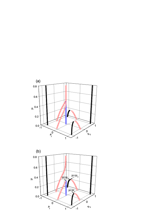
Figure 1: (color online) The stationary solutions of Eq.(1) in the absence of noises for $\sigma=0.0$ (a) and $\sigma=0.05$ (b). Stale node points, saddle points, and unstable node points are marked by solid squares, empty circles, and empty triangles, respectively.

To get a global view, in Fig.2 we plot the phase diagram in the $\mu-\sigma$ plane. The plane are divided into four different regions according to the number of solutions. As mentioned above, $\mu_{1}(\sigma)$, $\mu_{2}(\sigma)$, and $\mu_{3}(\sigma)$ are the separatrix between the region $n_{s}=9$ and the region $n_{s}=7$, between the region $n_{s}=7$ and the region $n_{s}=5$, and between the region $n_{s}=7$ and the region $n_{s}=3$, respectively. Both the region $n_{s}=7$ and the region $n_{s}=5$ have the shape of tongue. With decreasing $\sigma$ the region $n_{s}=7$ shrinks until it vanishes when the lines $\mu_{1}(\sigma)$ and $\mu_{2}(\sigma)$ get across at $\mu=0.195$ and $\sigma=0$. As $\sigma$ is increased, the region $n_{s}=5$ is reduced. For $\sigma=0.1$ the lines $\mu_{2}(\sigma)$ and $\mu_{3}(\sigma)$ are very close each other.

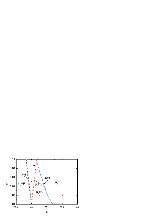
Figure 2: (color online) The property of solutions in the $\mu-\sigma$ plane. The plane are divided into four different regions according to the number of solutions, and boundary lines among neighboring regions are indicated by $\mu_{1}(\sigma)$, $\mu_{2}(\sigma)$, $\mu_{3}(\sigma)$, respectively.

Figure 3: (color online) Contour plots of the effective potential $V$ for four representative points marked by stars in Fig.2: $(\mu,\sigma)=(0.1,0)$ (a), $(0.2,0.05)$ (b), $(0.3,0.02)$ (c), and $(0.6,0.02)$ (d). Stale node points, saddle points, and unstable node points are marked by solid squares, empty circles, and empty triangles, respectively. The transition pathways are distinguished by the solid and dashed arrows. There is one saddle point for connecting any two stable node points.

In order to clearly exhibit the transition process at different regions, in Fig.3 we give the contour plots of the effective potential $V$ for four representative points $(\mu,\sigma)$ marked by stars in Fig.2. In the region $n_{s}=9$, there are two possible transition pathways, each of which contains a two-step transition process via an intermediate metastable state. Let $\Delta V_{1}^{(\alpha)}$ and $\Delta V_{2}^{(\alpha)}$ denote the energy barrier of the first step and the second step for the $\alpha$-th transition pathway ($\alpha=1,2$), respectively. The corresponding transition rates are

$${R^{(\alpha)}}=\frac{1}{{\frac{1}{{R_{1}^{(\alpha)}}}+\frac{1}{{R_{2}^{(\alpha)}}}}},$$ (6)

with

$$R_{1,2}^{(\alpha)}=Z\exp(-{{\Delta V_{1,2}^{(\alpha)}}\mathord{\left/{\vphantom{{\Delta V_{1,2}^{(\alpha)}}D}}\right.\kern-1.2pt}D}).$$ (7)

Here the prefactor $Z$ is given by Landauer and Swanson (1961)

$$Z={{\omega_{n}^{(1)}\omega_{n}^{(2)}{\omega_{s}^{(1)}}}\over{2\pi\omega_{s}^{(2)}}}.$$ (8)

Here $\omega_{s}^{(1,2)}=\sqrt{\left|{e_{s}^{(1,2)}}\right|}$ and $\omega_{n}^{(1,2)}=\sqrt{\left|{e_{n}^{(1,2)}}\right|}$ are the vibrational frequencies at the saddle point and at the node point from which the system escapes, where ${e_{s}^{(1,2)}}$ ($e_{s}^{(1)}<0$) and ${e_{n}^{(1,2)}}$ are the eigenvalues of Hessian matrix at the saddle point and at the node point, respectively,

The total transition rate is

$$R=p^{(1)}R^{(1)}+p^{(2)}R^{(2)},$$ (9)

where

$${p^{(1,2)}}=\frac{{R_{1}^{{}^{(1,2)}}}}{{R_{1}^{{}^{(1)}}+R_{1}^{{}^{(2)}}}}$$ (10)

are the probabilities of the two transition pathways happening.

In the region $n_{s}=7$, there are also two possible transition pathways. However, one pathway also contains a two-step process, but the other one becomes a one-step process. Let $\Delta V_{1}^{(1)}$ and $\Delta V_{2}^{(1)}$ denote the energy barrier of the first step and the second step for the two-step transition pathway, respectively, and $\Delta V^{(2)}$ the energy barrier for the one-step transition pathway. The total transition rate is also expressed by Eq.9, but we have

$$\left\{\begin{array}[]{l}{R^{(2)}}=Z\exp(-{{\Delta{V^{(2)}}}\mathord{\left/{\vphantom{{\Delta{V^{(2)}}}D}}\right.\kern-1.2pt}D})\\ {p^{(1)}}=\frac{{R_{1}^{{}^{(1)}}}}{{R_{1}^{{}^{(1)}}+{R^{(2)}}}}\\ {p^{(2)}}=\frac{{{R^{(2)}}}}{{R_{1}^{{}^{(1)}}+{R^{(2)}}}}\end{array}\right.$$ (14)

In the region $n_{s}=5$, there are also two possible transition pathways, but both of them contain a one-step process. Let $\Delta V^{(1)}$ and $\Delta V^{(2)}$ denote the energy barrier of the two transition pathways. The terms in the total transition rate by Eq.9 become

$$\left\{\begin{array}[]{l}{R^{(1,2)}}=Z\exp(-{{\Delta{V^{(1,2)}}}\mathord{\left/{\vphantom{{\Delta{V^{(1,2)}}}D}}\right.\kern-1.2pt}D})\\ {p^{(1,2)}}=\frac{{{R^{(1,2)}}}}{{{R^{(1)}}+{R^{(2)}}}}\end{array}\right.$$ (17)

Note that for the case $\sigma=0$, the two oscillators are identical and the two possible transition pathways are equivalent. However, as $\sigma$ is increased, the probability of the nucleation pathway marked by the solid line in Fig.3 quickly approaches one due to a larger force acted on the second oscillator, such that the total transition rate is almost determined by this dominant transition pathway.

Lastly, in the region $n_{s}=3$ there is a single one-step transition pathway. The nucleation rate is $R=Z\exp(-{{\Delta V}\mathord{\left/{\vphantom{{\Delta V}D}}\right.\kern-1.2pt}D})$, where $\Delta V$ is the energy barrier of the transition process.

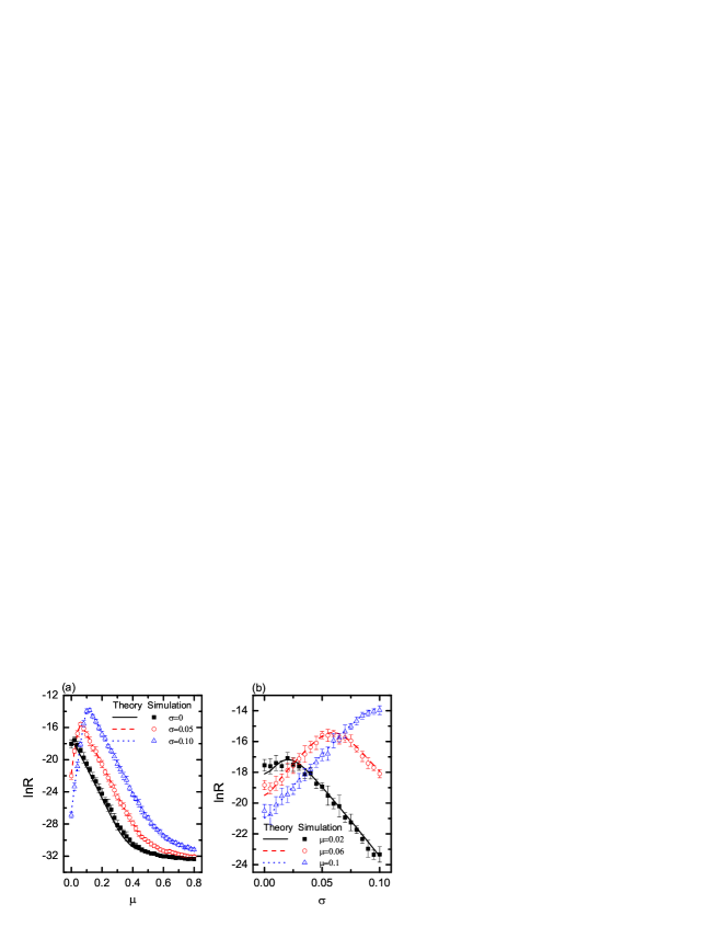
Figure 4: (color online) The logarithm of the total transition rate $\ln R$ as a function of $\mu$ for different $\sigma$ (a), and as a function of $\sigma$ for different $\mu$ (b). The theoretical results and FFS simulation ones are indicated by lines and symbols, respectively. The noise intensity is fixed at $D=0.01$.

So far, we have theoretically obtained the pathway and the rate of the transition in various parameters regions. For identical oscillators ($\sigma=0$), the system undergoes a transition from a two-step transition process with two possible pathways (transition in a serial way) to a one-step process with also two possible pathways at $\mu=\mu_{1}=\mu_{2}$ (transition in a synchronized way) to a one-step process with a single pathway at $\mu=\mu_{3}$. For nonidentical oscillators ($\sigma\neq 0$), a new transition way emerges at $\mu_{1}<\mu<\mu_{2}$ that is a candidate of a two-step pathway and a one-step pathway. In a word, in both cases there exists a critical coupling in which the transition changes from a two-step process to a one-step one. Interestingly, similar phenomenon was also reported in disturbed coupled nonlinear oscillators with purely deterministic dynamics Mezić (2006); Hennig et al. (2007); Hänggi et al. (2008); Eisenhower and Mezić (2010).

To validate the theory, we have performed extensive numerical simulations for Langevin equation 3. However, the transition is an activated process that occurs extremely slow, and brute-force simulation is thus prohibitively expensive. To overcome this difficulty, we will use a recently developed simulation method, forward flux sampling (FFS) Allen et al. (2005, 2009). All the simulation results are obtained via averaging over 20 independent FFS simulations.

In Fig.4(a), we show that the logarithm of the total transition rate $\ln R$ as a function of $\mu$ for different $\sigma$: $0$, $0.05$, and $0.1$. The theoretical results and FFS simulation ones are indicated by lines and symbols, respectively. There are an excellent agreement between them. For $\sigma=0$, $\ln R$ slightly increases and then decreases monotonically as $\mu$ is increased. Interestingly, if $\sigma$ becomes larger, for example $\sigma=0.5$, $\ln R$ clearly exhibits a nonmonotonic dependence on $\sigma$: $\ln R$ peaks at $\mu\simeq 0.06$. With further increasing $\sigma$, such a peak becomes more clear and the location of the peak shifts to a larger $\mu$. In Fig.4(b), we show that the dependence of $\ln R$ on $\sigma$ at different $\mu$. Clearly, $\ln R$ behaves significantly different dependence trend with $\sigma$ for different $\mu$. For $\mu<0.1$, $\ln R$ depends nonmonotonically on $\sigma$. There exists a maximal rate at a moderate magnitude of force disorder $\sigma$. On the other hand, for $\mu\geq 0.1$, $\ln R$ increases monotonically with $\sigma$. This implies that in the presence of a weak coupling a proper level of force mismatch can enhance the occurrence of the transition process. While for a relatively strong coupling, a larger magnitude of force mismatch is favorable to advance the process.

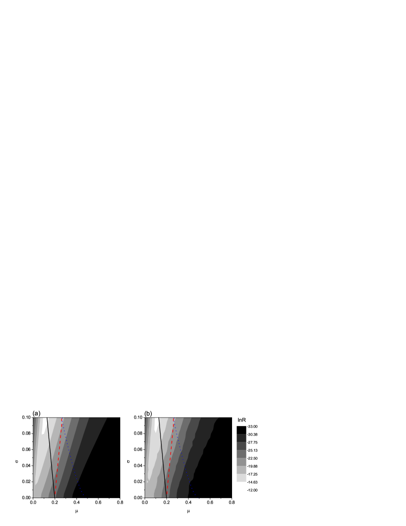
Figure 5: (color online) The contour plot of $\ln R$ in the $\mu-\sigma$ plane obtained by both theoretical calculation (a) and FFS simulations (b). The lines mark the separatrix as shown in Fig.2. The other parameter is $D=0.01$.

Furthermore, we summarize the results of $\ln R$ in the plane of parametric $\mu-\sigma$, as shown in Fig.5. The results are obtained both by theoretical calculation and by FFS simulations that are in good agreements. The region in which $\ln R$ is globally maximal appears near $(\mu,\sigma)\simeq(0.1,0.1)$, and the region $\ln R$ is globally minimal locates at the right bottom of the $\mu-\sigma$ plane. That is to say, if one wants to globally accelerate transition process, the force mismatch should be maximal while the coupling needs to be delicately chosen. If one intends to suppress the occurrence of transition, the force mismatch should be minimal and the coupling should be maximal.

IV Conclusions

To conclude, we have studied the transition process in a system of two mutually coupling forced bistable oscillators. By constructing the effective potential, we have shown that how the pathway and the rate of the transition change with the coupling strength and the force mismatch. We have identified four types of transition process at different parametric regions: (i) two possible transition pathways each containing a two-step transition process; (ii) two possible transition pathways one containing a two-step transition process and the other containing a one-step transition process; (iii) two possible transition pathways each containing a one-step transition process; (iv) a single one-step transition pathway. Furthermore, the total transition rate shows a rich dependence on coupling and force mismatch. On the one hand, as the coupling is strengthened the rate increases and then decreases, i.e., a maximal rate exists for an intermediate magnitude of coupling. On the other hand, the rate also shows a nonmonotonic dependence on the force mismatch for a weak coupling. While for a relatively strong coupling, the rate increases monotonically with the force mismatch. All the results have been validated to be in an excellent agreement with the extensive FFS simulations.

Obviously, partial results of the present work can give some valuable understanding for some existing phenomena reported previously Khasin et al. (2012a); Lombardo et al. (2014); Chen and Hou (2011); A. Nematzadeh and Ahn (2014); Mezić (2006). Meanwhile, our findings may provide potential implications for controlling transition events in coupled systems by a delicately chosen coupling or parametric mismatch. In the further work, the investigation of the more complex activated transition process in more than two coupled oscillators is desirable.