On Optimal Decision-Making in Ant Colonies

Abstract

Colonies of ants can collectively choose the best of several nests, even when many of the active ants who organize the move visit only one site. Understanding such a behavior can help us design efficient distributed decision making algorithms. Marshall et al. propose a model for house-hunting in colonies of ant Temnothorax albipennis. Unfortunately, their model does not achieve optimal decision-making while laboratory experiments show that, in fact, colonies usually achieve optimality during the house-hunting process. In this paper, we argue that the model of Marshall et al. can achieve optimality by including nest size information in their mathematical model. We use lab results of Pratt et al. to re-define the differential equations of Marshall et al. Finally, we sketch our strategy for testing the optimality of the new model.

1 Introduction

Understanding Collective Decision-Making (CDM) in human and animal groups can significantly help us design simple and efficient decentralized algorithms for distributed information systems. Decision making can be regarded as processing of uncertain information and producing a final choice among several alternatives. There is a dynamic tension between the speed and the accuracy of this process. The optimality of decision making process is often defined based on the trade-off between decision accuracy and decision speed. In other words, an optimal decision is a decision such that no other available decision options will result in a better trade-off between speed and accuracy.

The similarities between decision-making mechanisms in human brains and in colonies of social insects like ants are interesting: both systems are modeled with mutually interacting populations; in both systems, a decision is made when the size of one population exceeds some threshold; and in both systems, this threshold is adjusted to make a trade off between the decision speed and its accuracy. In the past two decades, these similarities have attracted the scientific community to study and model mechanisms of CDM in human and animal groups [7, 4, 3].

To the best of our knowledge, the best known model of biological CDM is due to Marshall et al. [3] who compare a model of decision-making in the primate brain with three models of CDM for house-hunting of social insect colonies. The first model, proposed by Pratt et al. [5], is related to the emigration of the rock ant Temnothorax albipennis, and the other two models are related to nest-site selection in the honeybee Apis mellifera. Among the models studied in [3], only direct-switching model of house-hunting by A. mellifera approximates optimal decision-making in a biologically plausible manner. Unfortunately, their ant model concludes that colonies of T. albipennis cannot achieve optimal decision-making.

In this paper, we argue that the non-optimal behavior shown by Marshall et al. [3] for the house-hunting CDM is not due to the inherent biological deficiencies but it is due to an unrealistic assumption in [3], where the ants do not consider nest size in their decision. Our goal is to build a new model of CDM in ant colonies with optimal decision-making for the house-hunting process. We do this by modifying the model of [3] to include nest size information. Similar to [3], we describe our model in terms of stochastic differential equations, which help us understand the collective behavior in situations with uncertainty.

As our long-term goal, we envision distributed decision-making algorithms based on our model for house-hunting in ant colonies. Such algorithms can be used in several applications including distributed task allocation, multi-agent systems, supply chain management, and auctions.

2 Preliminaries

In this section, we first describe a well-known approach for modeling CDM called diffusion model. Then, we describe the ants house-hunting CDM algorithm and the mathematical model of Marshall et al. [3].

Diffusion Model.

In this model, decisions are made by a noisy process that accumulates information over time toward one of the two alternatives. The model can be thought of as a random walk with normally distributed step size along a line. Each positive or negative direction corresponds to increasing evidence for one of the available alternatives. The random walk is subject to a constant drift, a tendency to move along the line towards the better alternative, whose strength is the difference between the expectations of the incoming information on the available alternatives. The noise in the accumulation of information is represented as the variance in the random walk.

The diffusion model of decision-making implements Sequential Probability Ratio Test (SPRT) developed by [8] and proved it achieves optimal decision-making over two alternatives [3], i.e., by varying the decision threshold it can compromise between speed and accuracy of decision-making. At the first step, SPRT assume a pair of hypotheses,$H_{1}:p=p_{0}$ and $H_{2}:p=p_{1}$. The next step is to gather evidence for the two alternative hypotheses and calculate the cumulative sum of the log-likelihood ratio, $\log\Lambda_{i}$, as new data arrive $S_{i}=S_{i-1}+\log\Lambda_{i}$. Finally, the stopping rule is a simple threshold scheme when the log of the likelihood ratio exceeds a positive or negative threshold. Through an adjustment of this threshold, the test can achieve the optimal trade-off between decision accuracy and speed. The use of log of the likelihood ratio ensures this test minimizes decision time for any desired decision error rate.

Ants House-Hunting Algorithm.

House-hunting of ant T. albipennis has been extensively studied as an interesting CDM behavior [5, 1, 6, 2]. Each colony of T. albipennis has a single queen and up to about 400 workers as well as brood (eggs, larvae, and pupae) that the colony has to rear. In the process of house-hunting, scouting ants first discover new nests and assess them according to some criteria such as size and darkness. Then, the scouts recruit nest-mates to the new nest using tandem-running, where an informed ant leads a second ant to her destination to get a second opinion about the nest. When the number of ants in the new nest reaches a threshold, scouts begin rapid transport of the rest of the colony by carrying nest-mates and brood. In each time step of the house-hunting process, each ant is in one of these three states: explore, tandem, and transport. The transition between these states happens based on the ant’s evaluation of the quality of the nest sites and the population of the ants in this sites [6]. By conducting laboratory experiments, Pratt et al. [6] have observed the following transition behaviors among T. albipennis ants.

1. If the ant is in the explore state and she has found a new site, she starts evaluating it. If the site is good, the ant switches to the state tandem.

2. If the ant is in the tandem state and the evaluation of the tandem follower is negative (i.e., the site is not good), the tandem leader switches to the explore state. If the follower’s evaluation is positive, then with probability $\frac{P^{k}}{P^{k}+T^{k}}$ the leader switches to the transport state, where $P$ is the nest population, $T$ is the population at which the probability is 0.5, and $k$ determines the non-linearity of the response, with higher $k$ yielding a more step-like function [6].

3. If the ant is in the transport state, she continues evaluating the site. If she finds a problem with the site, she switches to the explore state.

The transition from tandem to transport is interesting for us since it proves that the number of ants in a site is an important factor in the ant house-hunting process. We talk about this fact more in section 3.

House-Hunting Model of Marshall et al.

Marshall et al. [3] simplify the house-hunting model of [5] by defining the following factors.

1. Uncommitted scouting ants $s$, discover nest site $i$ and become recruiters $y_{i}$ at rate $q_{i}$. This rate is proportional to the quality of nest size and ease of discovery. Moreover, this rate is subject to noise $\eta_{q_{i}}$. This is modeled by the term $s\cdot(q_{i}+c\eta_{q_{i}})$ in the equations.

2. Recruiters $y_{i}$ for site $i$ recruit uncommitted scouts in class $s$ at a noisy quality-dependent rate $r{}_{i}^{\prime}$ with noise $\eta_{r{}_{i}^{\prime}}$. This is modeled $y_{i}\cdot(r{}_{i}^{\prime}+\eta_{r{}_{i}^{\prime}})$.

3. Recruiters for a site $i$ spontaneously switch to recruiting for the other site $j$ at rate $r_{i}$ subject to noise $\eta_{r_{i}}$. This is modeled by $y_{j}\cdot(r_{j}+\eta_{r_{j}})-y_{i}\cdot(r_{i}+\eta_{r_{i}})$.

4. Recruiters $y_{i}$ for a site $i$ spontaneously become uncommitted to any site at rate $k_{i}$ subject to noise $\eta_{k_{i}}$. This is modeled by $-y_{i}\cdot(k_{i}+\eta{k_{i}})$.

For two possible nest sites, the ants CDM process can be described by the following differential equations

$$\left\{\begin{array}[]{l}\dot{y_{1}}=s\cdot(q_{1}+c\eta_{q_{1}})+y_{1}\cdot(r^{\prime}_{1}+\eta_{r^{\prime}_{1}})+y_{2}\cdot(r_{2}+\eta_{r_{2}})-y_{1}\cdot(r_{1}+\eta_{r_{1}})-y_{1}\cdot(k_{1}+\eta{k_{1}})\\ \dot{y_{2}}=s\cdot(q_{2}+c\eta_{q_{2}})+y_{2}\cdot(r^{\prime}_{2}+\eta_{r^{\prime}_{2}})+y_{1}\cdot(r_{1}+\eta_{r_{1}})-y_{2}\cdot(r_{2}+\eta_{r_{2}})-y_{2}\cdot(k_{2}+\eta{k_{2}})\end{array}\right.,$$

where $s=n-y_{1}-y_{2}$.

3 Suggested Model

The house-hunting model of Marshall et al. [3] assumes that T. albipennis ants have no information about their colony size and the number of ants living in their own nest. In other words, the ants are unaware of the number of ants who are committed to the same nest or still uncommitted to any nest and are in the process of searching or waiting. In contrast, as shown by Pratt et al [6], the ants have a sense of these values and can decide based on them. The new model is described as follows.

1. Dependency to the number of uncommitted scouts. In [3], recruiters $y_{i}$ switch to the uncommitted state independent of the number of uncommitted scouts. Also, recruiting uncommitted scouts in class $s$ is performed independent of the number of uncommitted scouts. This means that by having more committed scouts to site $i$, the probability of switching from uncommitted to committed is fixed. However, we believe this probability decreases until all scouts commit to the same nest.

2. Dependency to the number of scouts in the their current site. In [3], recruiters of site $i$ start recruiting for site $j$ independent of the size of $j$. In contrast, we believe ants have some idea about their colony size and can observe how many ants have gathered in one site. In our model, ants use this size information for committing to nests.

Pratt et al. [6] argue that the probability of switching to the transport state is a step function of the normalized nest population. This probability is almost zero if the number of ants in the nest is smaller than a threshold, and it is close to one if this number is larger than a threshold, i.e.,

$$\Pr(\mathsf{transport})=\left\{\begin{array}[]{ll}0,&\quad\textrm{if }y_{i}\leq T\\ 1,&\quad\textrm{if }y_{i}>T\end{array}\right.,$$

where $y_{i}$ is the number of ants in site $i$, and $T$ is a fixed threshold parameter. Since transportation is approximately three times faster than tandem-running, this step function affects the number of uncommitted scouts that recruiters $y_{i}$ of site $i$ recruit. Thus, we can replace the term $y_{i}\cdot(r^{\prime}_{i}+\eta_{r^{\prime}_{i}})$ in the model of [3] with

$$\textrm{Number of scouts recruited by recruiters $y_{i}$= }\left\{\begin{array}[]{ll}y_{i}\cdot(r^{\prime}_{i}+\eta_{r^{\prime}_{i}}),&\quad\textrm{if }y_{i}\leq T\\ 3y_{i}\cdot(r^{\prime}_{i}+\eta_{r^{\prime}_{i}}),&\quad\textrm{if }y_{i}>T\end{array}\right..$$

Since it is not easy to use this step function directly in our differential equations, we estimate the function using the following polynomial computed using Matlab’s curve-fitting tool.

$$f(y_{i})=82.58y_{i}^{5}-205.33y_{i}^{4}+172.32y_{i}^{3}-54.03y_{i}^{2}+5.71y_{i}-0.11$$

Figure 1 shows this polynomial and the estimation used by Pratt et al. [6] calculated using the probability $\frac{P^{k}}{P^{k}+T^{k}}$.

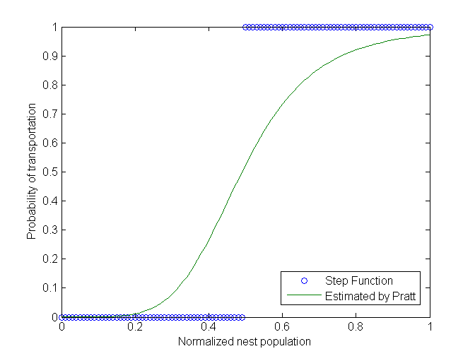
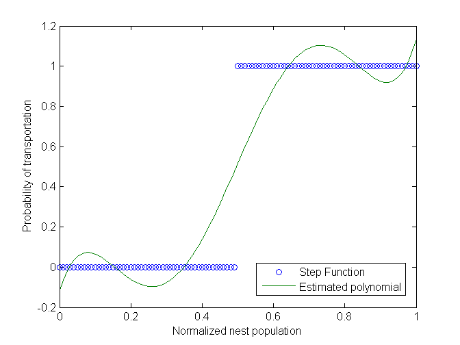
Figure 1: Estimation of the step function used by Pratt et al. [6] (left) and using a degree-five polynomial (right)

We now argue that unlike the model of Marshall et al. [3], our model achieves optimal CDM for the house-hunting process among ants T. albipennis. First, we define the model as stochastic differential equations.

1. Uncommitted scouts $s$ discover nest site $i$ and become recruiters $y_{i}$ at rate $q_{i}$. This rate is proportional to the size of nest and ease of discovery. Moreover, this rate is subject to noise $\eta_{q_{i}}$. This is modeled as $s(q_{i}+c\eta_{q_{i}})$.

2. Recruiters $y_{i}$ for site $i$ recruit uncommitted scouts in class $s$ at a noisy quality-dependent rate $r^{\prime}_{i}$ with noise $\eta_{r^{\prime}_{i}}$. This is modeled as $y_{i}\cdot(r^{\prime}_{i}+\eta_{r^{\prime}_{i}})\cdot(82.58y_{i}^{5}-205.33y_{i}^{4}+172.32y_{i}^{3}-54.03y_{i}^{2}+5.71y_{i}+0.9)$.

3. Recruiters for a site $i$ spontaneously switch to recruiting for the other site $j$ at rate $r_{i}$ subject to noise $\eta_{r_{i}}$. This is modeled as $y_{j}\cdot(r_{j}+\eta_{r_{j}})-y_{i}\cdot(r_{i}+\eta_{r_{i}})$.

4. Recruiters $y_{i}$ for a site $i$ spontaneously uncommitted to any site at rate $k_{i}$ subject to noise $\eta_{k_{i}}$. This is modeled as $-y_{i}\cdot(k_{i}+\eta{k_{i}})$.

For two possible nest sites, the ants decision-making process can be represented by the following equations,

$$\left\{\begin{array}[]{l}\dot{y_{1}}=s\cdot(q_{1}+c\eta_{q_{1}})+y_{1}\cdot(r^{\prime}_{1}+\eta_{r^{\prime}_{1}})\cdot(82.58y_{1}^{5}-205.33y_{1}^{4}+172.32y_{1}^{3}-54.03y_{1}^{2}+5.71y_{1}+0.9)\\ \quad+y_{2}\cdot(r_{2}+\eta_{r_{2}})-y_{1}\cdot(r_{1}+\eta_{r_{1}})-y_{1}\cdot(k_{1}+\eta{k_{1}})\\ \\ \dot{y_{2}}=s\cdot(q_{2}+c\eta_{q_{2}})+y_{2}\cdot(r^{\prime}_{2}+\eta_{r^{\prime}_{2}})\cdot(82.58y_{2}^{5}-205.33y_{2}^{4}+172.32y_{2}^{3}-54.03y_{2}^{2}+5.71y_{2}+0.9)\\ \quad+y_{1}\cdot(r_{1}+\eta_{r_{1}})-y_{2}\cdot(r_{2}+\eta_{r_{2}})-y_{2}\cdot(k_{2}+\eta{k_{2}})\end{array},\right.$$ (1)

where $s=n-y_{1}-y_{2}$.

We now briefly describe the steps required for the proof of optimality. First, we need to transform our model (Equation 1) into the new system $x_{1}\times x_{2}$, where $x_{1}=\frac{y_{1}-y_{2}}{\sqrt{2}},x_{2}=\frac{y_{1}+y_{2}}{\sqrt{2}}$ and $\dot{x_{1}}=\frac{\dot{y_{1}}-\dot{y_{2}}}{\sqrt{2}},\dot{x_{2}}=\frac{\dot{y_{1}}+\dot{y_{2}}}{\sqrt{2}}$. Applying these equations to the model gives

$$\left\{\begin{array}[]{l}\dot{x_{1}}=\frac{n}{\sqrt{2}}(q_{1}+-q_{2}+\sqrt{2}c\eta_{q})+\frac{f_{1}(\frac{\sqrt{}2}{2}(x_{1}+x_{2}))-f_{2}(\frac{\sqrt{}2}{2}(x_{2}-x_{2}))}{\sqrt{2}}\\ \quad+x_{1}\frac{(n-\sqrt{2}x_{2})(r^{\prime}_{1}+r^{\prime}_{2})+\sqrt{2}c\eta_{r^{\prime}}-k_{1}-k_{2}+\sqrt{2}c\eta_{k}-2r_{1}-2r_{2}+2\sqrt{2}c\eta_{r}}{2}\\ \quad+x_{2}\frac{(n-\sqrt{2}x_{2})(r^{\prime}_{1}-r^{\prime}_{2})+\sqrt{2}c\eta_{r^{\prime}}-k_{1}+k_{2}+\sqrt{2}c\eta_{k}-2r_{1}-2r_{2}-2\sqrt{2}c\eta_{r}+2q_{1}-2q_{2}+2\sqrt{2}c\eta_{q}}{2}\\ \\ \dot{x_{2}}=\frac{n}{\sqrt{2}}(q_{1}+q_{2}+\sqrt{2}c\eta_{q})+\frac{f_{1}(\frac{\sqrt{}2}{2}(x_{1}+x_{2}))+f_{2}(\frac{\sqrt{}2}{2}(x_{2}-x_{1}))}{\sqrt{2}}\\ \quad+x_{1}\frac{(n-\sqrt{2}x_{2})(r^{\prime}_{1}-r^{\prime}_{2})+\sqrt{2}c\eta_{r^{\prime}}-k_{1}+k_{2}+\sqrt{2}c\eta_{k}}{2}\\ \quad+x_{2}\frac{(n-\sqrt{2}x_{2})(r^{\prime}_{1}+r^{\prime}_{2})+\sqrt{2}c\eta_{r^{\prime}}-k_{1}-k_{2}+\sqrt{2}c\eta_{k}-2q_{1}-2q_{2}+2\sqrt{2}c\eta_{q}}{2}\end{array},\right.$$

where $f_{i}(x)=(r^{\prime}_{i}+\eta_{r^{\prime}_{i}})(82.58x^{6}-205.33x^{5}+172.32x^{4}-54.03x^{3}+5.71x^{2})$. Unfortunately, we cannot simply set the exponent of $x_{1}$ and $x_{2}$ to zero because of the $f_{i}(x)$ terms in the equations. Similar to [3], it is required to check if this equation can asymptotically approximate the constant drift diffusion model. To this end, we need to fix a value for $x_{2}$ independent of $x_{1}$ and then, analyze the behavior of $\dot{x_{1}}$.

4 Discussion and Conclusion

We defined new differential equations for the house-hunting process among ants based on the dependency to the number of scouts in the nests. We justified our model by referring to the empirical results of Pratt et al. [6]. Finally, we sketched our strategy for testing the optimality of the new model.

One major difference between our model and the model of Marshall et al. [3] is that they assume the decision-making process terminates once the ants start the transportation phase. However, we believe that the transportation step is an important part of the decision-making process and can significantly affect the result of the process. Switching from the tandem state to transport state happens when the number of ants in the nest is larger than a threshold and the probability of this transition is a step function which can be estimated by a polynomial of degree five. At the early stage of the process, the ants in both nests are in the tandem state. Once the population of the nest reaches a threshold, the ants may switch the transport state which can happen in both nests. This transition from one state to another should not be assumed as a termination signal because, in fact, the ants may change their decision and go back to tandem state or even switch to a new nest.

Adding the transport state to the model makes this equations dependent to the nest size which shows itself in having a polynomial of degree five in equations. Later on in testing the optimality, this change shows itself to have terms dependent to both $x_{1}$ and $x_{2}$ and make it impossible to have the random process $\dot{x_{1}}$ independent to $x_{2}$ and itself which rejects the result of [3]. However, it is the first step in the proof of optimality.

Our main challenge for the future is to complete our proof of optimality, which we envision to require steps similar to those described in Appendix D of [3]. We are also interested in checking consistency of the predictions made by our model to empirical results obtained from simulations of the house-hunting CDM. Moreover, we are interested in a probabilistic model of the house-hunting process where the expected number of ants in each nest is considered. This approach seems useful for checking if the ants find the best nest with high probability when the colony has enough time to choose between alternatives.

References

- [1] L. Conradt and T. Roper. Consensus decision making in animals. Trends in ecology & evolution, 20(8):449–456, 2005.
- [2] N. R. Franks, A. Dornhaus, C. S. Best, and E. L. Jones. Decision making by small and large house-hunting ant colonies: one size fits all. Animal Behaviour, 72, 2006.
- [3] J. Marshall, R. Bogacz, A. Dornhaus, R. Planqué, T. Kovacs, and N. Franks. On optimal decision-making in brains and social insect colonies. Journal of the Royal Society, Interface / the Royal Society, 6(40):1065–1074, 2009.
- [4] K. M. Passino, T. D. Seeley, and P. K. Visscher. Swarm cognition in honey bees. Behavioral Ecology and Sociobiology, 62(3):401–414, 2008.
- [5] S. C. Pratt, E. B. Mallon, D. J. Sumpter, and N. R. Franks. Quorum sensing, recruitment, and collective decision-making during colony emigration by the ant leptothorax albipennis. Behavioral Ecology and Sociobiology, 52(2):117–127, 2002.
- [6] S. C. Pratt, D. J. Sumpter, E. B. Mallon, and N. R. Franks. An agent-based model of collective nest choice by the ant temnothorax albipennis. Animal Behaviour, 70, 2005.
- [7] P. K. Visscher. Group decision making in nest-site selection among social insects. Annu. Rev. Entomol., 52:255–275, 2007.
- [8] A. Wald. Sequential tests of statistical hypotheses. The Annals of Mathematical Statistics, 16(2):117–186, 1945.