Pattern Recognition in a Ring of Delayed Phase Oscillators

Abstract.

We show that a ring of phase oscillators coupled with transmission delays can be used as a pattern recognition system. The introduced model encodes patterns as stable periodic orbits. We present a detailed analysis of the underlying dynamics. In particular, we show that the system possesses a multitude of periodic solutions, prove stability results and present a bifurcation analysis. Furthermore, we show successful recognition results using artificial patterns and speech recordings.

1. Introduction

The ability to recognize encoded patterns is a very general and omnipresent skill in humans and animals. Here, the term pattern can refer to a structure of any nature activating a sensory perception. However, recognition of visual and sonic patterns are the most common applications. Developing artificial pattern recognition systems as well as investigating actual natural mechanisms of pattern recognition in humans and animals has been a scientific challenge for decades [33, 12, 18, 34, 27, 22]. The most famous dynamical model is probably the one developed by Hopfield in 1982 [14]. It is a recurrent artificial neural network consisting of coupled discrete elements. In contrast to feedforward networks the underlying graph might have loops leading to more complex dynamics and multistability, which in turn is used to store several patterns in the network. Recently, there has been much effort in developing more realistic models of human pattern recognition [4, 35, 15]. It is evident that the pattern recognition task is closely related to the memory function, and there is a strong evidence that memory and memory recall are related to synchronization of neuronal ensembles [17]. On the other hand, in absence of stimuli parts of the brain are known to be in a desynchronized state [8]. Consequently, models under consideration mostly consist of coupled nonlinear dynamical systems that may possess complex dynamics [5, 39].

Delay coupled networks is another class of systems which attracted much attention recently. Even a system consisting of a single dynamical node with delayed feedback can be used effectively for information processing purposes as it is evidenced in [3, 20]. In [16] it is shown that a spiking network with delayed connections can exhibit reproducible time-locked but not synchronous firing patterns and the number of such patterns exceeds the number of neurons in the network by far. Indeed, there is an increasing evidence that the brain’s memory and retrieval functions are closely connected to spike timing [13].

Here, we present an evidence that pattern recognition tasks can be performed by a system consisting of a single loop of delay coupled phase oscillators. In contrast to the Hopfield model, patterns in this model are not stored as fixed points but as periodic orbits. In this way, time dimension is introduced in the information processing device, which is biologically plausible. We also mention that the simple ring structure makes it accessible to analytic investigations and, at the same time, it serves as a model for central pattern generators [11, 28, 29, 32]. The mechanism that we employ here is based on general properties of rings of time-delayed systems with different connection delays, described in [25, 37]. The delay transformation introduced therein is used for analyzing the appearance of different patterns in rings (as well as more complex networks [23]) with nonidentical delays.

The article is structured as follows. In section 2 we analyze the model equations with homogeneous delay. In particular, we study coexisting periodic solutions in such a system and their number and stability. Section 3 introduces the pattern recognition mechanism. In section 4 we apply the model to various signals ranging from simple artificial ones to speech and present numerical results. Section 5 concludes with a discussion and an outlook on various open questions.

2. Synchronous Motions In Rings Of Phase Oscillators

In this section we introduce the dynamical system used as a pattern recognition device and present some useful results concerning its dynamics. To our knowledge these results are new. We consider a delayed, unidirectional ring of phase oscillators

(2.1) $$\dot{x}_{j}\left(t\right)=\omega+\kappa\sin\left(x_{j+1}\left(t-\tau\right)-x_{j}\left(t\right)\right)$$

where $x_{j}\in 2\pi\mathbb{R}/\mathbb{Z}$ and all the oscillators have the same individual frequency $\omega$. The coupling between the oscillators is of strength $\kappa>0$ and delayed by a time delay $\tau>0$. Provided with a global coupling structure these equations are well known as Kuramoto model [19]. A lot of research has been done on the synchronization properties of Kuramoto oscillators with instantaneous coupling and related bifurcation scenarios since the 80s [2]. Similarly, delayed Kuramoto oscillators are well investigated [38, 21, 7], whereas there are fewer results on phase oscillators with a local coupling structure, neither with instantaneous [26, 30, 31] nor delayed coupling [9].

As our aim is to construct/memorize and recognize patterns by means of synchronous states, we first have to assure the existence of the synchronous solutions. We remark that by introducing new variables $y_{j}=x_{j}-\omega$ and rescaling the time $t\mapsto\kappa t$ system (2.1) transforms to $\dot{y}_{j}\left(t\right)=\sin\left(y_{j+1}\left(t-\tilde{\tau}\right)-y_{j}\left(t\right)\right)$. However, we will consider (2.1), since it does not make the analysis more complicated and still keeps the coupling strength and frequency explicitly.

2.1. Existence of synchronous periodic solutions

Synchronous periodic solutions of (2.1) are of the form

(2.2) $$x_{j}\left(t\right)=x_{s}(t)=\Omega t$$

for some mean frequency $\Omega\in\mathbb{R}$. Substituting this solution in system (2.1) yields the transcendental equation for $\Omega$

(2.3) $$\Omega=\omega-\kappa\sin\left(\Omega\tau\right).$$

Now, introducing the variable $z=\Omega\tau$ equation (2.3) transforms to

(2.4) $$\frac{z}{\kappa\tau}=\frac{\omega}{\kappa}-\sin(z)$$

That is, we look for intersections of a straight line through the origin with slope $\frac{1}{\kappa\tau}$ and a shifted sine, see Fig. 2.1 (a).

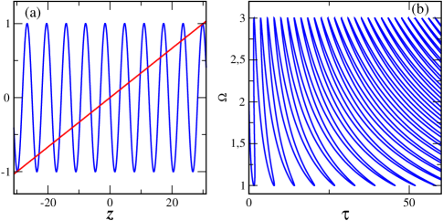
Figure 2.1. (a) Graphical representation of solutions to Eq. (2.4). The intersection points determine frequencies of synchronous solutions $\Omega$, $z=\Omega\tau$. Parameters: $\omega=0$, $\tau=10$, and $\kappa=3$. (b) Frequency of synchronous solutions versus delay $\tau$, given by Eq. (2.5). Parameters: $\omega=2$ and $\kappa=1$.

In order to visualize how multiple synchronous solutions (2.2) with different frequencies appear for different delay times $\tau$, let us represent the solutions of (2.3) in the following parametric form

(2.5) $$\tau\left(s\right) =\frac{s}{\omega+\kappa\sin\left(-s\right)}$$

$$\Omega\left(s\right) =\frac{s}{\tau\left(s\right)}$$

So the same branch of periodic solutions reappears slightly inclined for larger values of $\tau$, see Fig. 2.1 (b). Both figures show that indeed, either increasing $\tau$ or $\kappa$ leads to an increase of solutions of the form (2.2). Actually, it is known that the number of coexisting periodic solutions in systems with time delay $\tau$ grows at least linearly with $\tau$ [36]. In our case, using simple geometrical arguments, one can show that the number of such solutions is approximately $2\kappa\tau/\pi$. A proof together with the stability analysis is given in the following section.

2.2. Stability of synchronous solutions

The main result of this section is, that half of the above mentioned $2\kappa\tau/\pi$ synchronous solutions are linearly stable, whereas the other half is unstable. To determine the linear stability consider the linearization of equation (2.1) along a synchronous solution of the form (2.2)

$$\dot{\xi}\left(t\right)=-K\xi\left(t\right)+KG\xi\left(t-\tau\right),$$

where $K=\kappa\cos\left(\Omega\tau\right)$ and $G=\{g_{ij}\}$ is the adjacency matrix of the unidirectional ring coupling, i.e. $g_{ij}=1$ if $j=i+1\,\mbox{mod}\,N$ and $g_{ij}=0$ otherwise. Here $N$ is the number of oscillators in the ring. Thus the linear stability is given by the distribution of zeros $\mu$ of the following characteristic equation

$$F\left(\mu\right) = \det\left(-\mu\mbox{Id}-K\mbox{Id}+Ke^{-\mu\tau}G\right)$$

$$= -\left(\mu+K\right)^{N}+K^{N}e^{-N\mu\tau}.$$

The solutions $\mu$ of this equation are the characteristic exponents (eigenvalues) whose real parts determine the stability. The obtained characteristic equation can be factorized to the set of $N$ more simple equations:

(2.6) $$0=\mu+K-Ke^{-\mu\tau}e_{n},\quad n=0,\dots,N-1,$$

where $e_{n}=\exp\left[i2\pi n/N\right]$ are $N$-th roots of unity. Now we can prove the following lemma.

Lemma 1.

Let $x\left(t\right)=\Omega t$ be a synchronous solution of (2.1). The solution is linearly stable iff the following condition holds

$$\cos\left(\Omega\tau\right)>0.$$

Furthermore, if $\cos\left(\Omega\tau\right)<0$, the following upper bound for the real parts of the characteristic exponents $\mu$ holds true

$$\Re\left(\mu\right)\leq-2\kappa\cos\left(\Omega\tau\right).$$

Proof.

Splitting equation (2.6) into real and imaginary parts ($\mu=x+iy$) yields

(2.7) $$0 = x+K\left(1-e^{-x\tau}\cos\left(\frac{2\pi n}{N}-y\tau\right)\right),$$

$$0 = y-Ke^{-x\tau}\sin\left(\frac{2\pi n}{N}-y\tau\right).$$

Consider the two cases $K>0$ and $K<0$:
i) Case $K>0$. For $x>0$ we have $x+K\left(1-e^{-x\tau}\cos\left(\frac{2\pi n}{N}-y\tau\right)\right)>0$ which contradicts equation (2.7). Consequently, equation (2.7) can only be fulfilled for $x<0$. It is shown in [9] that $K>0$ is also a necessary condition for stability which concludes the proof of the first part of the lemma.
ii) Case $K<0$. If we have $x\leq 0$ the upper bound is automatically valid. So suppose we have a solution $\left(x,y\right)$ with $x>0$. Then the equation (2.7) implies

$$0<-K\left(1-e^{-x\tau}\cos\left(\frac{2\pi n}{N}-y\tau\right)\right)<-2K,$$

so for $x>-2K$ we would have $x+K\left(1-e^{-x\tau}\cos\left(\frac{2\pi n}{N}-y\tau\right)\right)>0$ which means that indeed, the real part $x$ of $\mu$ can be bounded as follows

$$x\leq-2K=-2\kappa\cos\left(\Omega\tau\right).$$

∎

Using the condition for stability from lemma 1 we obtain estimations for the number of coexistent stable and unstable periodic orbits.

Lemma 2.

Let $2\tau\kappa>\pi$. Then there are at least $\frac{\kappa\tau}{\pi}-\frac{1}{2}$ stable and unstable periodic synchronous solutions of equation (2.1), respectively.

Proof.

Finding periodic solutions is equivalent to finding zeros of the function $f\left(\Omega\right)=\Omega-\omega+\kappa\sin\left(\Omega\tau\right)$. We have seen in the last lemma, that a solution with frequency $\Omega$ is stable if $\cos\left(\Omega\tau\right)>0$. This is the case for $\Omega\tau\in\left(-\frac{\pi}{2},\frac{\pi}{2}\right)+2\pi l$. Motivated by this we define the disjoint intervals

$$I_{l} = \left(-\frac{\pi}{2\tau},\frac{\pi}{2\tau}\right)+\frac{2\pi l}{\tau}\qquad l\in\mathbb{Z},$$

$$J_{l} = \left(\frac{\pi}{2\tau},\frac{3\pi}{2\tau}\right)+\frac{2\pi l}{\tau}\qquad l\in\mathbb{Z},$$

for which $\cos\left(\Omega\tau\right)>0$ and $\cos\left(\Omega\tau\right)<0$, respectively. We first remark that we have to fulfill $\Omega\in\left(\omega-\kappa,\omega+\kappa\right)$ (see equation (2.3)). A straightforward calculation shows that the number $M$ of intervals $I_{l}$ lying in $\left(\omega-\kappa,\omega+\kappa\right)$ satisfies

$$\frac{\kappa\tau}{\pi}-\frac{1}{2}\leq M\leq\frac{\kappa\tau}{\pi}+\frac{1}{2}.$$

Now in $I_{l}$ we have

$$f^{\prime}\left(\Omega\right)=1+\kappa\tau\cos\left(\Omega\tau\right)>0$$

and further $f\left(-\frac{\pi}{2\tau}+\frac{2\pi l}{\tau}\right)\leq 0\leq f\left(\frac{\pi}{2\tau}+\frac{2\pi l}{\tau}\right)$ for all $I_{l}\subset\left(\omega-\kappa,\omega+\kappa\right)$. So $f$ has exactly one zero in each $I_{l}$ by monotonicity. By the same argument there has to be an odd number of zeros in each $J_{l}$. By the shape of $f$ we conclude that it has one zero in each $J_{l}$ as well. So the total number of zeros $m$ in intervals $J_{l}$ has the same bounds as $M$. ∎

2.3. Bifurcations of synchronous solutions

In subsection 2.1 we have seen that synchronous solutions undergo bifurcations as either the delay time $\tau$ or the coupling strength $\kappa$ is varied. In this section we give some insight into these bifurcations. A solution (2.2) can change its stability when one of its characteristic exponents crosses the imaginary axis $\mu=iy$, $y\in\mathbb{R}$. Substituting $\mu=iy$ into (2.6) and splitting the obtained equation into real and imaginary parts yields

(2.8) $$0 =K\left(1-\cos\left(\frac{2\pi n}{N}-y\tau\right)\right),$$

$$0 =y-K\sin\left(\frac{2\pi n}{N}-y\tau\right).$$

The first equation in (2.8) is fulfilled if either $K=0$ or $\frac{2\pi n}{N}-y\tau=2\pi l$ for some $l\in\mathbb{Z}$. Plugged into the second equation both conditions yield $y=0$. Thus, Hopf bifurcations with $y\neq 0$ cannot occur in the model. The only possible destabilization corresponds to eigenvalues crossing the imaginary axis with vanishing imaginary part $y$. On the other hand, every periodic solution has a trivial characteristic exponent $\mu=0$ corresponding to perturbations in the direction of the periodic motion. So in order to look for a change of stability we have to find non-simple zeros of the characteristic function. Such non-simple zeros are possible if $F^{\prime}\left(0\right)=-NK^{N-1}\left(K\tau+1\right)=0$. This is fulfilled if either one of the following conditions holds

(2.9) $$K =0,$$

$$\tau K =-1.$$

The following lemma describes the type of bifurcations taking place if the conditions (2.9) hold, see also Fig. 2.2. We remind that $K=\kappa\cos(\Omega\tau)$.

Lemma 3.

Let $x_{\tau}\left(t\right)=\Omega\left(\tau\right)t$ be a branch of synchronous solutions of equation (2.1) with $\kappa\neq 0$. Varying $\tau$ it undergoes a transcritical bifurcation at $K=0$. If $\omega\neq\pi l\kappa$ for any $l\in 2\mathbb{Z}+1$ it undergoes a fold bifurcation at $K=-1/\tau$ with $K$ defined as above.

Proof.

As it was mentioned above, under conditions (2.9) an eigenvalue crosses the imaginary axis with vanishing imaginary part. So the observed bifurcations can either be transcritical or fold. In a fold bifurcation two new solutions emerge. This happens exactly when the right hand side in (2.3) crosses the identity (see Fig. 2.1(a)), which is equivalent to

$$1 = \frac{\partial}{\partial\Omega}\left[\omega-\kappa\sin\left(\Omega\tau\right)\right]$$

$$= -\tau\kappa\cos\left(\Omega\tau\right)=-\tau K$$

This condition also shows that at $K=0$ no other solution emerges, therefore, the bifurcation at $K=0$ is transcritical. A straightforward calculation shows that the eigenvalues cross the imaginary axis with nonzero speed indeed.

∎

Fig. 2.2 shows the obtained bifurcation diagram for synchronous solutions, including the stability information. Here we used that for $\tau=0$ we have $K=\kappa>0$, so the synchronous state is stable.

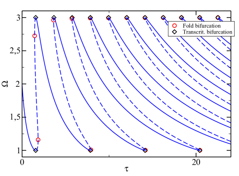
Figure 2.2. Bifurcation diagram for synchronous solutions (2.2). Frequency $\Omega$ is plotted versus time delay $\tau$. Dotted lines represent unstable and plain lines stable solutions. Parameters: $\omega=2$, $\kappa=1$. With increasing $\tau$, the two bifurcations, transcritical and fold, are converging to each other.

We remark that, requiring $\sum_{j}a_{ij}=R\,,\,\forall i$ and appropriate conditions on $f$, the above analysis can be done for the more general system

$$\dot{x}_{j}\left(t\right)=\omega+\frac{\kappa}{R}\sum_{j=1}^{N}a_{ij}f\left(x_{j}\left(t-\tau\right)-x_{i}\left(t\right)\right)$$

with similar results. For the linear stability see [9].

3. Pattern Recognition

In this section we present the idea of how pattern recognition can be realized with the ring of delay coupled oscillators. We have seen in the previous section that system (2.1) admits coexisting synchronous solutions $x_{j}^{i}\left(t\right)=\Omega_{i}t$ with frequencies $\left\{\Omega_{i}\right\}_{i\in I}\subset\left(\omega-\kappa,\omega+\kappa\right)$ given by equation (2.3). In analogy with the firing times of neuronal systems [10, 6] we pay special attention to the moments when an oscillator $x_{j}^{i}\left(t\right)$ reaches the boundary of the periodic domain $\left[0,2\pi\right]$, i.e. $x_{j}\left(t_{j}\right)=2\pi$. This choice of phase is arbitrary, and any other phase $\varphi_{*}$ instead of $2\pi$ can be chosen instead [24]. In what follows, we will use the obtained crossing time sequences $t_{j}$ to represent patterns. In section 3.1 we explain how a given pattern can be encoded in a ring of phase oscillators, see Fig. 3.1. Afterwards, in section 3.2 we explain the dynamic recognition process.

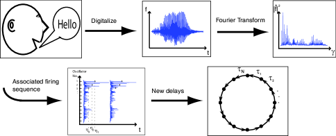
Figure 3.1. The process chart visualizes the encoding mechanism. Step one is the recording and digitalization of a given stimulus. The second step is not mandatory for pattern encoding. However, we employ it in this article as it yields better results. It consists of a fast Fourier transformation (FFT) of the recorded stimulus. Then, a firing sequence $P$ is associated to the Fourier transform such that each value of the FFT’s square modulus is identified with the firing time of an element of the ring. The last step is calculating the coupling delays in the ring according to (3.3), so the resulting dynamical system admits the firing sequence $P$ as a stable solution.

3.1. Encoding

The idea for encoding a pattern in a ring of delay coupled oscillators is based on a time shift transformation [37, 25]. We shortly describe it here. We assume that a pattern $P$ is represented by some $N$-dimensional vector $P=\left(p_{1},p_{2},...,p_{N}\right)\in\mathbb{R}^{N}$. First, let us choose an $\Omega_{i}$ that corresponds to a stable synchronous solution of (2.1). The timeshift transformation

(3.1) $$y_{j}\left(t\right)=x_{j}\left(t-p_{j}\right)$$

converts (2.1) to the system

(3.2) $$\dot{y}_{j}\left(t\right)=\omega+\kappa\sin\left(y_{j+1}\left(t-\tau_{j}\right)-y_{j}\left(t\right)\right),$$

which has the same form as (2.1) except that the new delays

(3.3) $$\tau_{j}:=\tau-\left(p_{j+1}-p_{j}\right)$$

are non-identical. Here we assume that $\tau_{j}\geq 0$, which is always possible by taking $\tau$ sufficiently large. Under the transformation (3.1), the synchronous state $x_{j}\left(t\right)=\Omega_{i}t$ transforms into the solution

$$y_{j}\left(t\right)=\Omega_{i}\cdot\left(t-p_{j}\right)$$

of system (3.2). The stability properties of this solution are also preserved [23]. Thus, in the system with non-homogeneous delays (3.2), an oscillator $j$ crosses the phase $2\pi$ at times $p_{j},p_{j}+\frac{2\pi}{\Omega_{i}},...$. Consequently, changing the delays $\tau\mapsto\tau_{j}$ yields the new system system (3.2) that exhibits exactly the required crossing sequence $P$ as a stable periodic solution. In particular, the encoding is not a dynamic process but just consists of the calculation of the $N$ delays $\tau_{j}$.

3.2. Recognition

Now suppose $P$ is encoded as described above. Let

$$Q=P+\left(\delta_{1},\delta_{2},...,\delta_{N}\right)$$

be a perturbed version of pattern $P$ that is to be recognized. We associate an initial function for system (3.2) in a natural manner

$$y^{0}\left(t\right)=\Omega_{i}\cdot\left(t-q_{1},t-q_{2},....,t-q_{N}\right)$$

So for $\delta_{i}=0$ it corresponds to the synchronous state $\Omega_{i}t$ itself in transformed coordinates. Then, the recognition task consists of deciding whether $Q$ is recognized as the previously encoded pattern $P$. In order to do so we start system (3.2) with the initial function $y^{0}$ associated to $Q$ and stop after a fixed time $T$. Then some measure of similarity between $\Phi_{T}\left(Q\right)$, which is $Q$ evolved under the flow of (3.2), and $P$ is considered to decide whether $Q$ should be recognized as $P$. To specify the measure of similarity employed here, consider the following straightforward calculation. Transformed back in original coordinates the initial function $y^{0}$ reads

$$x_{j}^{0}\left(t\right) = y_{j}^{0}\left(t+p_{j}\right)$$

$$= \Omega_{i}\left(t+p_{j}-q_{j}\right)$$

$$= \Omega_{i}\left(t-\delta_{j}\right).$$

This means that solving system (3.2) with initial function $y^{0}$ (corresponding to $Q$) is equivalent to solving the original system (2.1) with initial function $x_{j}^{0}\left(t\right)$ (corresponding to $\Delta=\left(\delta_{1},\delta_{2},...,\delta_{N}\right)$). In other words, pattern $Q$ is recognized as version of $P$ if the orbit with initial function $x_{j}^{0}\left(t\right)$ corresponding to $Q$ converges fast enough to the synchronous state with frequency $\Omega_{i}$ (where “fast enough” has to be quantified in a specific situation). Consequently, we can use the order parameter $r\left(t\right)=\sum_{j=1}^{N}\left|e^{i\Phi_{t}\left(x^{0}\right)}\right|$ as measure of similarity (reference and/or explain here?). It is worth stressing the fact that the essential parameters for the pattern recognition are the time $T$ after which we stop simulation of the differential equations and a threshold for the order parameter that lets us decide whether the flow after time $T$ is close enough to the synchronous state, that is whether the pattern is recognized or not. The choice of these parameters constitutes the learning phase.

4. Numerical Results

In this section we present numerical results for pattern recognition. An important quantity for the mechanism is the size and shape of the basin of attraction of the stable periodic solution representing the encoded pattern, as the basin contains initial conditions (patterns) that are possibly identified with the encoded pattern (see Fig. 4.1 (b)). Obviously, we can not present a complete picture of the basins of attraction as the phase space is infinite dimensional. However, we will address some aspects of this question numerically in the following sections.

4.1. Recognition of artificial patterns

We start with a simple pattern $P=\left(2,1,...,1\right)$. Fig. 4.1 shows the order parameter after time $T=90$ for initial values $P+Q_{j}$, where $Q_{j}=\left(0,...,0,\underbrace{\varepsilon}_{j},0,...,0\right)$. Here $j$ determines the location and $\varepsilon$ the size of the perturbation. We observe that, from a certain index $j$ on, initial values $P+Q_{j}$ converge to the pattern with the same speed.

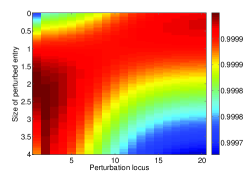
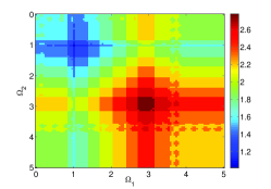
Figure 4.1. (a) Encoded pattern $\left(2,1,...,1\right)$. Initial values are $P+Q_{j}$ with $Q_{j}=\left(0,...,0,\underbrace{\varepsilon}_{j},0,...,0\right)$, where $j$ determines the location and $\varepsilon$ the size of the perturbation. Color codes the order parameter measured after time $T=900$. Parameters are $\tau=3,$ $\omega=1,$ $\kappa=1$. (b) Visualization of attractor basins for two oscillators. The axis correspond to initial values $\left[\Omega_{1}t,\Omega_{2}t\right]$. Color codes the frequency of synchronous motion at time $T=50000$. Parameters are $\omega=2$, $\kappa=1$ and $\tau=20$. For this value of $\tau$ we observe thirteen coexisting synchronous states of which seven are stable which can be seen in Fig. 2.2.

As a preparation for more complex audio signals we next investigate recognition of simple sine waves. The task is the following: Suppose two sine waves of different frequencies are encoded as two patterns $P_{1}$ and $P_{2}$. It is to decide whether a given third wave $Q$ is recognized as either one of the two encoded sines. Here, we proceed as described in the flow chart Fig. 3.1. According to our scheme, the corresponding Fourier transforms $P_{1}$ and $P_{2}$ are the pattern associated with the signals. The use of Fourier transform has the following advantages: one can cut off the transformed signal above a certain frequency which can be seen as a simple denoising process and at the same time it accelerates the recognition process. Furthermore, for short enough time windows the time course of the signal is not important and the Fourier transform contains the main information independent of the signal’s exact timing. The pattern associated to a sine wave of a fixed frequency $f$ is a delta peak $\delta_{f}$ (in an ideal case without noise). It is evident that the error tolerance does not depend on the absolute value of the frequency $f$ but rather on the frequency difference of the perturbation and the pattern to be identified.

Fig. 4.2 shows the results of two different recognition processes. In the first recognition (a) two sine waves of 5Hz and 15Hz are encoded. Again, the recognition process consists of deciding whether a third given sine wave is recognized as either one. It can be seen in the lower left plot that the 5Hz and the 15Hz wave are recognized with an error tolerance of $\pm$0.1Hz. The same results hold for recognition of the standard pitch A (440Hz) and one semitone higher ($\sim$466Hz) (Figure (b)). In both cases the order parameter is measured after time $T=50$ which corresponds to $\sim$17 times the delay time $\tau=3$. So the recognition is still relatively fast.

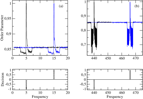
Figure 4.2. Pattern recognition with two encoded sine waves of frequencies 5Hz and 15Hz (a) and 440Hz and 466Hz (b). A third wave which is to be recognized is used as initial value for the system transformed according to the 5Hz and 15Hz patterns respectively (see flow chart 3.1). Upper plots show order parameters after time $T=50$ for the different recognition processes. Parameters are $\tau=3,\,\omega=1,\,\kappa=1$. Lower plots show decision of the PR device. $-1$ stands for “Pattern 1 is chosen”, $1$ for “Pattern 2 is chosen” and $0$ for none.

4.2. Speech Recognition

In this section, we use the model for speech recognition. As above for sine waves, the pattern associated to an audio signal is its Fourier transform. This is done to circumvent that otherwise, two identical signals with different timing would not be recognized as the same. With the transformed patterns we proceed in the same way as described in section 3. The original audio signals are the numbers from one to ten, spoken by two different voices (male and female), each in three takes. So in total it is a set of 60 audio tracks. First we encoded two randomly chosen different recordings. For the recognition we randomly chose one of the four remaining recordings that coincide with one of the two encoded numbers. In the previous training phase we set the parameters to $\omega=1$, $\kappa=1$, $\tau=3$, and $T=25$. The resulting recognition process was successful with a rate of around 75%.

5. Conclusion

In this article, we have presented an evidence that a ring of delay coupled oscillators can be used for information processing purposes. In contrast to other models, the encoding of patterns is particularly simple. For a signal of length $N$ it just consists of $N$ point operations, the calculation of the new delays, in contrast to the Hopfield model which requires the definition of $N^{2}$ coupling weights. Furthermore, arbitrary patterns can be encoded. In section 2 we presented an extensive system’s analysis. Using these results the model can be controlled easily and parameters can be tuned suited to the application on hand. Particularly, the number of stable periodic orbits can be controlled and chosen arbitrarily high. Their frequencies, bounded from below and above by $\omega-\kappa$ and $\omega+\kappa$ respectively, can be easily determined numerically by solving the transcendent equation 2.3. Results from section 4 show that the model can be used as a reliable device for simple artificial pattern recognition as well as for single word speech recognition.

The aim of this article was to introduce main ideas, present some analytical results for the model, as well as its potential capability for information processing. Consequently, there are still open questions and paths for future research. Here, we just mention a few. In section 2 it was shown that for larger values of the delay $\tau$ the model possesses a large number of coexisting stable periodic orbits. This fact could possibly be exploited further. Furthermore, considering Fourier transforms as patterns for speech recognition was a probable choice, but possibly not the best. It is an open question which preprocessing procedure suits best for the model on hand. When classifying a pattern into two classes, we simply measured the distance of the pattern to the two classes after a fixed time by calculating the order parameter. This, of course, can be generalized to more than two classes. Numerical results show that considering the cross correlation instead of the order parameter yield similar results. Yet, it is unclear which distance measure is best for a certain class of signals. Furthermore, one could even think of coupling different rings representing different classes in some way to yield a single object representing a composite of classes. More generally the construction above is still feasible for arbitrary coupling topologies. We only presented results for artificial and audio signals. Encoding 2-D visual patterns should be possible using the same ideas for a 2-D lattice.

References

- [1]
- [2] J. A. Acebrón, L. L. Bonilla, C. J. Pérez Vicente, F. Ritort, and R. Spigler. The Kuramoto model: A simple paradigm for synchronization phenomena. Rev. Mod. Phys., 77:137–185, 2005.
- [3] L. Appeltant, M. C. Soriano, G. Van der Sande, J. Danckaert, S. Massar, J. Dambre, B. Schrauwen, C. R. Mirasso, and I. Fischer. Information processing using a single dynamical node as complex system. Nature Comm, 2, 2011.
- [4] R. M. Borisyuk. Spiking neural network mode for memorizing sequences with forward and backward recall. BioSystems, 112:214–223, 2013.
- [5] A. B. Breve, L. Zhao, M. G. Quiles, and E. E. N. Macau. Chaotic phase synchronisation and desynchronization in an oscillator network for object selection. Neur. Netw., 22(5-6):728–737, 2009.
- [6] C.C. Canavier and S. Achuthan. Pulse coupled oscillators and the phase resetting curve. Mathematical biosciences, 226(2):77–96, 2010.
- [7] M. Chen, Y. Shang, Y. Zou, and J. Kurths. Synchronization in the kuramoto model: A dynamical gradient network approach. Phys. Rev. E, 77:027101, Feb 2008.
- [8] G. Deco, V. K. Jirsa, and R. McIntosh. Emerging concepts for the dynamical organization of resting-state activity in the brain. Nature Reviews Neuroscience, 12:43–56, 2011.
- [9] M.G. Earl and S.H. Strogatz. Synchronization in oscillator networks with delayed coupling: A stability criterion. Phys. Rev. E, 67:036204, 2003.
- [10] P. Goel and B. Ermentrout. Synchrony, stability, and firing patterns in pulse-coupled oscillators. Physica D: Nonlinear Phenomena, 163(3-4):191 – 216, 2002.
- [11] M. Golubitsky, I. Stewart, P.L. Buono, and J.J. Collins. Symmetry in locomotor central pattern generators and animal gaits. Nature, 401:693–695, 1999.
- [12] S. Grosberg. Competitive learning: From interactive activation to adaptive resonance. Cognitive Science, 11:23–63, 1987.
- [13] M. E. Hasselmo, L. M. Giocomo, and M. Yoshida. Cellular dynamical mechanisms for encoding the time and place of events along spatiotemporal trajectories in episodic memory. Behavioral Brain Research, 215, 2:261–274, 2010.
- [14] J. J. Hopfield. Neural networks and physical systems with emergent collective computational abilities. Proc Natl Acad Sci U S A, 79:15541558, 1982.
- [15] J. J. Hopfield and C. D. Brody. Sequence reproduction, single trial learning and mimicry based on a mammalian-like distributed code for time. Arxiv, -:–, 2009.
- [16] E. M. Izhikevich. Polychronization: Computation with spikes. Neural Computation, 18:245–282, 2006.
- [17] W. J. Jermakowicz and V. A. Casagrande. Neural networks a century after cajal. Brain Research Reviews, 55:264–284, 2007.
- [18] T. Kohonen. Self-Organizing Maps. Springer, 2001.
- [19] Y. Kuramoto. Chemical Oscillations, Waves, and Turbulence. Springer, Berlin, 1984.
- [20] L. Larger, M. C. Soriano, D. Brunner, L. Appeltant, J. M. Gutierrez, L. Pesquera, C. R. Mirasso, and I. Fischer. Photonic information processing beyond turing: an optoelectronic implementation of reservoir computing. Opt. Express, 20(3):3241–3249, Jan 2012.
- [21] W. S. Lee, E. Ott, and T. M. Antonsen. Large coupled oscillator systems with heterogeneous interaction delays. Phys. Rev. Lett., 103:044101, Jul 2009.
- [22] X. Liang and L. Zhao. Phase-noise-induced resonance in arrays of coupled excitable neural models. IEEE Trans. on Neural Networks and Learning Systems, 24:1339–1345, 2013.
- [23] L. Lücken, J. P. Pade, K. Knauer, and S. Yanchuk. Reduction of interaction delays in networks. EPL (Europhysics Letters), 103:10006, 2013.
- [24] O. Popovych, S. Yanchuk, and P. Tass. Self-organized noise resistance of oscillatory neural networks with spike timing-dependent plasticity. Scientific Reports, (accepted).
- [25] O. V. Popovych, S. Yanchuk, and P. A. Tass. Delay- and coupling-induced firing patterns in oscillatory neural loops. Phys. Rev. Lett., 107:228102, 2011.
- [26] J. A. Rogge and D. Aeyels. Stability of phase locking in a ring of unidirectionally coupled oscillators. Journal of Physics A: Mathematical and General, 37:11135–11148, 2004.
- [27] T.C. Silva and L. Zhao. Network-based high level data classification. IEEE Trans. on Neural Networks and Learning Systems, 23:954–970, 2012.
- [28] N. Strelkowa and M. Barahona. Transient dynamics around unstable periodic orbits in the generalized repressilator model. Chaos, 21(2):023104, 2011.
- [29] A. Takamatsu, R. Tanaka, H. Yamada, T. Nakagaki, T. Fujii, and I. Endo. Spatiotemporal symmetry in rings of coupled biological oscillators of physarum plasmodial slime mold. Phys. Rev. Lett, 87(7):078102, Jul 2001.
- [30] P. F. C. Tilles, F. F. Ferreira and H. A. Cerdeira. Multistable behavior above synchronization in a locally coupled Kuramoto model. Phys. Rev. E, 83:066206, 2011
- [31] P. F. C. Tilles, F. F. Ferreira and H. A. Cerdeira. Local attractors, degeneracy and analyticity: Symmetry effects on the locally coupled Kuramoto model. Chaos, Solitons & Fractals, 49:32–46, 2013
- [32] A. Vishwanathan, G. Bi, and H.C. Zeringue. Ring-shaped neuronal networks: a platform to study persistent activity. Lab Chip, 11(6):1081–8, 2011.
- [33] C. von der Malsburg. The correlation theory of brain function. Technical report, Max-Planck-Institute for Biophysical Chemistry, 1981.
- [34] DeLiang Wang. Time dimension for scene analysis. IEEE Trans. on Neural Networks and Learning Systems, 16:1401–1426, 2005.
- [35] Y. Yamaguchi. A theory of hippocampal memory based on theta phase precession. Biological Cybernetics, 89:1–9, 2003.
- [36] S. Yanchuk and P. Perlikowski. Delay and periodicity. Phys. Rev. E, 79(4):046221, 2009.
- [37] S. Yanchuk, P. Perlikowski, O. V. Popovych, and P. A. Tass. Variability of spatio-temporal patterns in non-homogeneous rings of spiking neurons. Chaos, 21:047511, 2011.
- [38] M. K. Stephen Yeung and Steven H. Strogatz. Time delay in the kuramoto model of coupled oscillators. Physical Review Letters, 82(3):648–651, Jan 1999.
- [39] L. Zhao, J. C. G. Caceres, A. P. G. Damiance Jr., and H. Szu. Chaotic dynamics for multi-value content adressable memory. Neurocomputing, 69:1628–1636, 2006.