ABSTRACT. We study the statistics of backward clusters in a gas of hard spheres at low density. A backward cluster is defined as the group of particles involved directly or indirectly in the backwards–in–time dynamics of a given tagged sphere. We derive upper and lower bounds on the average size of clusters by using the theory of the homogeneous Boltzmann equation combined with suitable hierarchical expansions. These representations are known in the easier context of Maxwellian molecules (Wild sums). We test our results with a numerical experiment based on molecular dynamics simulations.

KEYWORDS. Low–density gas, homogeneous Boltzmann equation, backward cluster, Boltzmann hierarchy.

1 Introduction

Consider a system of $N$ identical hard spheres of diameter $\varepsilon$ moving in the whole space ${\mathbb{R}}^{3}$ or in a bounded box with reflecting boundary conditions. The collisions between spheres are governed by the usual laws of elastic reflection. We order the particles with an index $i=1,2,\cdots,N$. A configuration of the system is ${\bf z}_{N}=(z_{1},\cdots,z_{N})$, where $z_{i}=(x_{i},v_{i})$ are the position and the velocity of particle $i$ respectively. Let us assign a probability density $W_{0}^{N}$ on the $N-$particle phase space, assuming it symmetric in the exchange of the particles, and let $W^{N}(t)$ be its time evolution according to the hard sphere dynamics. Finally, for $j=1,2,\cdots,N$, denote by $f^{N}_{0,j}$ and $f^{N}_{j}(t)$ the $j-$particle marginals of $W_{0}^{N}$ and $W^{N}(t)$ respectively.

Given a tagged particle, say particle $1$, consider $z_{1}(t,{\bf z}_{N})$ its state (position and velocity) at time $t$ for the initial configuration ${\bf z}_{N}$. We define the backward cluster of particle $1$ (at time $t$ and for the initial configuration ${\bf z}_{N}$) as the set of particles with indices $J\subset I_{N}$, where $I_{N}=\{1,2,\cdots,N\}$, constructed in the following way. Going back in time starting from $z_{1}(t,{\bf z}_{N})$, let $i_{1}$ be the (index of the) first particle colliding with $1$. Next, considering the two particles $1$ and $i_{1}$, let us go back in time up to the first collision of one particle of the pair with a new particle $i_{2}$ and so on up to time $0$. Then $J=\{i_{1},i_{2},\cdots,i_{n}\}$ with $i_{r}\neq i_{s}$ for $r\neq s$. We denote by $K$ the cardinality of $J$, i.e., $K=|J|$.

In this paper we are interested in studying the quantity $\langle K\rangle_{t}$ that is the average (with respect to the initial distribution) of the cardinality of the backward cluster of a tagged particle at time $t$. In a general context this is a hard task, however we limit ourselves in considering $\langle K\rangle_{t}$ in a low–density situation, namely in the Boltzmann–Grad limit [5, 6]

$$N\to\infty,\quad\varepsilon\to 0\quad\mbox{and}\quad N\varepsilon^{2}\to\lambda^{-1}>0\;,$$ (1.1)

where $\lambda$ is a constant proportional to the mean free path. We fix $\lambda=1$ in the rest of the paper.

Moreover, we shall assume that the initial distribution is approximately factorized, namely the marginals of the initial distributions do factorize in the Boltzmann–Grad limit, and that the one particle distribution is independent of $x$.

In this situation it is believed (and in fact proved for short times and under suitable uniform estimates on the $f^{N}_{0,j}$) that the system is ruled by the homogeneous Boltzmann equation, which we remind here for the unknown $f=f(v,t)$:

$$\partial_{t}f(v,t)=\int_{{\mathbb{R}}^{3}\times S^{2}_{+}}dv_{1}d\omega\ (v-v_{1})\cdot\omega\Big{\{}f(v_{1}^{\prime},t)f(v^{\prime},t)-f(v_{1},t)f(v,t)\Big{\}}$$ (1.2)

where $S_{+}^{2}=\{\omega\in S^{2}|\ (v-v_{1})\cdot\omega\geq 0\},$ $S^{2}$ is the unit sphere in ${\mathbb{R}}^{3}$ (with surface measure $d\omega$), $(v,v_{1})$ is a pair of velocities in incoming collision configuration and $(v^{\prime},v_{1}^{\prime})$ is the corresponding pair of outgoing velocities defined by the elastic reflection rules

$$\begin{cases}\displaystyle v^{\prime}=v-\omega[\omega\cdot(v-v_{1})]\\ \displaystyle v_{1}^{\prime}=v_{1}+\omega[\omega\cdot(v-v_{1})]\end{cases}\;.$$ (1.3)

The Cauchy theory of equation (1.2) is well known, see [15] and references quoted therein. The solution $f=f(v,t)$ is usually interpreted as the one–particle distribution of the system in the low–density regime.

In the next section we will give a precise definition for the quantity $\langle K\rangle_{t}$ associated to the Boltzmann equation (1.2). In order to describe the long time behaviour of $\langle K\rangle_{t}$, it will be convenient to focus on:

$$r=\lim_{t\to\infty}\frac{1}{t}\log\langle K\rangle_{t}\;.$$ (1.4)

In Section 3 we shall compute exactly $\langle K\rangle_{t}$ and $r$ for a simplified model of Maxwellian molecules. In this case $r$ is an absolute constant. In Sect. 4 we come back to the hard sphere system and prove an exponential estimate of the growth in time of $\langle K\rangle_{t}$. However the rate is not constant anymore, but depends on the initial datum.

A comparison of $\langle K\rangle_{t}$, $r$ with the corresponding quantities at the level of the particle system ($\varepsilon>0$) will be performed numerically in Section 5.

The cluster dynamics outside the low–density regime has been studied previously, both analytically [13, 14] as regards the equilibrium dynamics of infinite particle systems, and numerically [4]. In the latter reference, recent applications to several domains are mentioned and discussed, such as plasma physics, geophysics or economics.

We stress however that the notion of cluster introduced in these papers (see e.g. [4], Section 2) differs from that of “backward cluster” considered in the present work . This refers exclusively to the backward dynamics of one single tagged particle. In particular, note that the particles join a backward cluster one by one. In other words, when particle $i$ joins the backward cluster of particle $1$, the particles belonging to the backward cluster of $i$, not involved in the backward cluster of $1$, are ignored.

This concept emerges naturally from the perturbative description of the Boltzmann–Grad limit, as enlightened in the following section, and is related to the Markovian character of the dynamics.

We conclude this introduction by observing that the interest on the control of the backward cluster is also related to the problem of “mathematical validity of the Boltzmann equation”. It is known that the validity of the Boltzmann equation is crucially dependent on the factorization of the marginals of the $N-$particle system $f^{N}_{j}({\bf v}_{j},t)$, where ${\bf v}_{j}=(v_{1},\cdots,v_{j})$, at any positive time $t$. In order that this property is fulfilled, it is necessary that the backward clusters of any couple of particles (say $1$ and $2$) are disjoint. When such two clusters are finite, the probability that the two particles are dynamically correlated is $O\left(\frac{\langle K\rangle_{t}^{2}}{N}\right)$. We estimate in Sect. 4 $\langle K\rangle_{t}$ assuming that the Boltzmann–Grad limit has been achieved. Therefore this result can be interpreted as a compatibility argument.

Another connected problem is the following. Even though the convergence $f^{N}_{j}({\bf v}_{j},t)\to f(v_{1},t)f(v_{2},t)\cdots f(v_{j},t)$ in the Boltzmann–Grad limit has been proven at least for short times [7], one can wonder for which $j$ the asymptotic equivalence holds. If the $j$ particles have finite backward clusters, we can argue that the probability of correlations between any pair in the group of $j$ particles is $O(\frac{j^{2}}{N})$. Therefore we expect that the factorization property of marginals holds when $\lim_{N}\frac{j^{2}}{N}=0$. Actually in [10] it has been proven that the propagation of chaos holds for short times if $j\leq N^{\alpha}$ for $\alpha$ small enough.

Finally it may be worth noting that the notion of backward cluster could be of interest in problems of population dynamics where one is interested in the mean growth of a group of individuals which contacted, directly or indirectly, a given one.

2 Preliminaries: the Boltzmann-Grad limit

In what follows we expand the solution of (1.2), i.e. $f(v,t)$, in terms of a sum

$$f=\sum_{n=0}^{\infty}f^{(n)}\;,$$ (2.1)

where $f^{(n)}$ is interpreted as the contribution to the probability density $f$ due to the event: the backward cluster of $1$ has cardinality $n$.

Let $f_{0}=f_{0}(v)$ be the initial datum for the Boltzmann equation. By (1.2) it follows naturally that

$$f^{(0)}(v,t)=e^{-\int_{0}^{t}dsR(v,s)}f_{0}(v),$$ (2.2)

where

$$R(v,t)=\int_{{\mathbb{R}}^{3}\times S^{2}_{+}}dv_{1}d\omega\ (v-v_{1})\cdot\omega f(v_{1},t)=\pi\int_{{\mathbb{R}}^{3}}dv_{1}|v-v_{1}|f(v_{1},t)\;.$$ (2.3)

Before giving the other terms of the expansion we introduce a useful tool, namely the Boltzmann hierarchy.

Suppose that $f$ is a solution to the Boltzmann equation (1.2) and consider the products

$$f_{j}({\bf v}_{j},t)=f(t)^{\otimes j}({\bf v}_{j})=f(v_{1},t)f(v_{2},t)\cdots f(v_{j},t)\;,$$ (2.4)

where ${\bf v}_{j}=(v_{1},\cdots,v_{j})$. The family of $f_{j}$ solves then the hierarchy of equations

$$\partial_{t}f_{j}({\bf v}_{j},t)={\cal C}_{j+1}f_{j+1}({\bf v}_{j},t)-R_{j}({\bf v}_{j},t)f_{j}({\bf v}_{j},t)\;,$$ (2.5)

where

$${\cal C}_{j+1}=\sum_{k=1}^{j}{\cal C}_{k,j+1}$$ (2.6)

$${\cal C}_{k,j+1}f_{j+1}({\bf v}_{j},t)=\int_{{\mathbb{R}}^{3}\times S^{2}_{+}}dv_{j+1}d\omega\,(v_{k}-v_{j+1})\cdot\omega\,f_{j+1}(v_{1},\cdots,v^{\prime}_{k},\cdots,v_{j},v^{\prime}_{j+1},t)\;,$$

$$\begin{cases}\displaystyle v^{\prime}_{k}=v_{k}-\omega[\omega\cdot(v_{k}-v_{j+1})]\\ \displaystyle v^{\prime}_{j+1}=v_{j+1}+\omega[\omega\cdot(v_{k}-v_{j+1})]\end{cases}\;,$$ (2.7)

$$S^{2}_{+}=\{\omega\ |\ (v_{k}-v_{j+1})\cdot\omega\geq 0\}\;,$$

and

$$R_{j}({\bf v}_{j},t)=\sum_{k=1}^{j}R(v_{k},t)\;.$$ (2.8)

By using a formal solution of (2.5) iteratively, we can express $f_{j}(t)$ via the following series

$$f_{j}(t)=\sum_{n\geq 0}\int_{0}^{t}dt_{1}\int_{0}^{t_{1}}dt_{2}\cdots\int_{0}^{t_{n-1}}dt_{n}$$

$$\ \ \ \ \ \ \ \ \ \ \ \ \ \ \ \ \cdot\SS_{j}(t_{1},t){\cal C}_{j+1}\SS_{j+1}(t_{2},t_{1})\cdots{\cal C}_{j+n}\SS_{j+n}(0,t_{n})f_{0}^{\otimes(j+n)}\;,$$ (2.9)

where we use the conventions $t_{0}=t,t_{n+1}=0$, and the term $n=0$ should be interpreted as $\SS_{j}(0,t)f_{0}^{\otimes j}$. Here $\SS_{j}(t_{1},t_{2})$ is the multiplicative operator defined as

$$\SS_{j}(t_{1},t_{2})f_{j}({\bf v}_{j},\cdot)=e^{-\int_{t_{1}}^{t_{2}}dsR_{j}({\bf v}_{j},s)}f_{j}({\bf v}_{j},\cdot)\;.$$ (2.10)

Note that in (2.9), and in the formulas below, the dependence on ${\bf v}_{j}$ is not shown explicitly.

In more detail,

$$f_{j}(t)=\sum_{n\geq 0}\sum_{k_{1},\cdots,k_{n}}\int_{0}^{t}dt_{1}\int_{0}^{t_{1}}dt_{2}\cdots\int_{0}^{t_{n-1}}dt_{n}$$

$$\ \ \ \ \ \ \ \ \ \ \ \ \ \ \ \ \cdot\SS_{j}(t_{1},t){\cal C}_{k_{1},j+1}\SS_{j+1}(t_{2},t_{1})\cdots{\cal C}_{k_{n},j+n}\SS_{j+n}(0,t_{n})f_{0}^{\otimes(j+n)}\;,$$ (2.11)

where $k_{1}\in\{1,\cdots,j\},k_{2}\in\{1,\cdots,j+1\},\cdots,k_{n}\in\{1,2,\cdots,j+n-1\}$. We call any sequence $\{k_{1},\cdots,k_{n}\}$ of this type a “$j-$particle tree with $n$ creations”. Indeed any new created particle in formula (2.11), say $j+r$, can be attached to any of the previous $j+r-1$ particles (for more details on this representation, see e.g. [10]). We denote a $j-$particle tree with $n$ creations by $\Gamma_{n}(j)$.

Fixed $\Gamma_{n}(j)$, $\omega_{1},\cdots,\omega_{n}$, ${\bf v}_{j}$ and the velocities of the new particles $v_{j+1},\cdots,v_{j+n}$, we introduce a sequence of vector velocities ${\bf v}^{s}$, $s=0,\cdots,n$, by setting:

$${\bf v}^{0}={\bf v}_{j},\quad{\bf v}^{s}=(v_{1}^{s-1},\cdots,v_{k_{s}}^{\prime},\cdots,v_{j+s-1}^{s-1},v_{j+s}^{\prime})\quad s\geq 1$$

where, at step $s$, the pair $v_{k_{s}}^{\prime},v_{j+s}^{\prime}$ are the pre–collisional velocities (in the collision with impact vector $\omega_{s}$) of the pair $v_{k_{s}}^{s-1},v_{j+s}^{s-1}$ (which are, by construction, post–collisional). This allows to write (2.11) more explicitly as

$$f_{j}(t)=\sum_{n\geq 0}\sum_{\Gamma_{n}(j)}\int_{0}^{t}dt_{1}\cdots\int_{0}^{t_{n-1}}dt_{n}\int_{{\mathbb{R}}^{3n}}dv_{j+1}\cdots dv_{j+n}e^{-\int_{t_{1}}^{t}ds\,R_{j}({\bf v}_{j},s)}\,$$

$$\ \ \ \left(\prod_{r=1}^{n}\int_{(v^{r-1}_{k_{r}}-v_{j+r})\cdot\omega_{r}\geq 0}d\omega_{r}\,(v^{r-1}_{k_{r}}-v_{j+r})\cdot\omega_{r}\,e^{-\int_{t_{r+1}}^{t_{r}}ds\,R_{j+r}({\bf v}^{r},s)}\right)f_{0}^{\otimes(j+n)}({\bf v}^{n})\;,$$

where we are using the convention $t_{n+1}=0$.

Formula (2.9) expresses the solution to the Boltzmann equation (1.2) in terms of an expansion on the number of collisions. Each term of the series is the contribution to $f_{j}$ due to the event in which the first $j$ particles and the collided particles in the backward dynamics deliver exactly $n$ collisions. Setting $f_{j}=\sum_{n}f^{(n)}_{j}$, we identify

$$f_{j}^{(n)}(t)=\int_{0}^{t}dt_{1}\cdots\int_{0}^{t_{n-1}}dt_{n}\,$$ (2.13)

$$\cdot e^{-\int_{t_{1}}^{t}dsR_{j}(s)}{\cal C}_{j+1}e^{-\int_{t_{2}}^{t_{1}}dsR_{j+1}(s)}{\cal C}_{j+2}\cdots{\cal C}_{j+n}\,e^{-\int_{0}^{t_{n}}dsR_{j+n}(s)}f_{0}^{\otimes(j+n)}\;.$$

In particular (2.1) holds with

$$f^{(n)}(t)=\int_{0}^{t}dt_{1}\cdots\int_{0}^{t_{n-1}}dt_{n}$$ (2.14)

$$\cdot e^{-\int_{t_{1}}^{t}dsR_{1}(s)}{\cal C}_{2}e^{-\int_{t_{2}}^{t_{1}}dsR_{2}(s)}{\cal C}_{3}\cdots{\cal C}_{1+n}e^{-\int_{0}^{t_{n}}dsR_{1+n}(s)}f_{0}^{\otimes(1+n)}\;.$$

As a consequence, we define

$$\langle K\rangle_{t}=\sum_{n=0}^{\infty}n\int dv\,f^{(n)}(v,t).$$ (2.15)

A remarkable property which will be used later on is the following:

$$f_{2}^{(n)}=\sum_{\begin{subarray}{c}n_{1},n_{2}:\\ n_{1}+n_{2}=n\end{subarray}}f^{(n_{1})}f^{(n_{2})}\;.$$ (2.16)

This is consequence of the rather obvious identity

$$\sum_{\Gamma_{n}(2)}\int_{0}^{t}dt_{1}\cdots\int_{0}^{t_{n-1}}dt_{n}=\sum_{\begin{subarray}{c}n_{1},n_{2}:\\ n_{1}+n_{2}=n\end{subarray}}\,\sum_{\begin{subarray}{c}\Gamma_{n_{1}}(1)\\ \Gamma_{n_{2}}(1)\end{subarray}}\,\int_{0}^{t}dt_{1}^{1}\cdots\int_{0}^{t^{1}_{n_{1}-1}}dt^{1}_{n_{1}}\int_{0}^{t}dt^{2}_{1}\cdots\int_{0}^{t^{2}_{n_{2}-1}}dt_{n_{2}}\;.$$ (2.17)

As we shall discuss in the next section, the expansion (2) is a version of the Wild sums in the context of the hard sphere dynamics.

We expect $\langle K\rangle_{t}$ to be bounded for a fixed $t$ and exponentially growing in $t$, so that it is natural to introduce the quantities

$$r_{+}=\limsup_{t\to\infty}\frac{1}{t}\log\langle K\rangle_{t}$$ (2.18)

and

$$r_{-}=\liminf_{t\to\infty}\frac{1}{t}\log\langle K\rangle_{t}\;.$$ (2.19)

Note that $r_{\pm}$ are computed by using the macroscopic scale of times, in which the mean flight time is $O(1)$. We stress that the introduced quantities refer only to the kinetic reduced description, given by the homogeneous Boltzmann equation. The corresponding quantities at the level of the particle system ($\varepsilon>0$) are very difficult to handle with. In particular we have no results stating that such quantities are equivalent to (2.18), (2.19) in the Boltzmann–Grad limit. In the last section, we shall present related numerical simulations.

As we shall discuss later on, generally speaking we expect that $r_{+}=r_{-}=r$ defined as in (1.4).

The quantities we have introduced make sense also at equilibrium, namely when $f_{0}=M_{\beta}$ is a uniform Maxwellian with inverse temperature $\beta>0$. Presently we are not able to show, even in this case, that $r_{-}=r_{+}=r$. If this is true, observe that $r=r_{\beta}$ depends only on the temperature (or the energy) of the Maxwellian $M_{\beta}$. On the other hand, by virtue of the $H$ Theorem, any (non equilibrium) distribution $f_{0}$ with the same energy should have the same value of $r$. In the last section we will show some numerical evidence of this behaviour for the hard sphere system.

We observe further that the dependence on the temperature should be given by

$$r_{\beta}=\frac{r_{1}}{\sqrt{\beta}}\;.$$ (2.20)

This follows from $M_{\beta}(v)=\beta^{3/2}M_{1}(\sqrt{\beta}v)$ which implies, by (2.3) and (2.14), $R^{\beta}(v)=(1/\sqrt{\beta})R^{1}(\sqrt{\beta}v)$ and

$$f^{(n),\beta}(v,t)=\beta^{3/2}f^{(n),1}\left(\sqrt{\beta}v,\frac{t}{\sqrt{\beta}}\right)\;.$$

Here we have used an upper index to indicate the dependence on the temperature of the corresponding quantities. The last equation can be obtained easily from (2.14) by a rescaling of all the integration variables (times and velocities). It follows that $\langle K\rangle^{\beta}_{t}=\langle K\rangle^{1}_{t/\sqrt{\beta}}$, so that (2.20) holds if $r_{\beta}$ exists.

3 A simple model

In this section we briefly analyze a simplified model of the Boltzmann equation for Maxwellian molecules with angular cut–off [1], for which the computations of the mean cluster size $\langle K\rangle_{t}$ can be made explicitly.

We consider the Boltzmann equation

$$\partial_{t}f=J(f,f)-f$$ (3.1)

where

$$J(f,f)(v)=\int_{{\mathbb{R}}^{3}\times S^{2}}dv_{1}d\omega\ g\left(\cos\theta\right)f(v_{1}^{\prime})f(v^{\prime})$$ (3.2)

for some nonnegative function $g$ satisfying $g=0$ for $\cos\theta<0$, and

$$\cos\theta=\frac{(v-v_{1})}{|v-v_{1}|}\cdot\omega\;.$$

Note that we have fixed the time scale in such a way that

$$\int_{S^{2}}d\omega\,g(\cos\theta)=1\;.$$ (3.3)

Proceeding as in the previous section, we write the associated hierarchy

$$\partial_{t}f_{j}=J_{j+1}f_{j+1}-jf_{j}\;,$$ (3.4)

where $J_{j+1}$ is defined as ${\cal C}_{j+1}$ (see (2.6)) with the function $(v_{k}-v_{j+1})\cdot\omega$ replaced by $g\left(\frac{(v_{k}-v_{j+1})}{|v_{k}-v_{j+1}|}\cdot\omega\right)$. Again $f_{j}=f^{\otimes j}$ where $f=f(v,t)$ solves (3.1). The initial condition for (3.4) is $f_{0}^{\otimes j}$.

From (3.4) one deduces (the analogous of (2) for $j=1$)

$$f(v,t)=\sum_{n\geq 0}\sum_{\Gamma_{n}(1)}\int_{0}^{t}dt_{1}\cdots\int_{0}^{t_{n-1}}dt_{n}\int_{{\mathbb{R}}^{3n}}dv_{2}\cdots dv_{1+n}\int_{S^{2n}}d\omega_{1}\cdots d\omega_{n}$$

$$\ \ \ \ \ \ \ \ \ \ \ \ \ \ \ \ \ \cdot g(\cos\theta_{1})\cdots g(\cos\theta_{n})e^{-(t-t_{1})}e^{-2(t_{1}-t_{2})}\cdots e^{-(n+1)t_{n}}f_{0}^{\otimes(1+n)}({\bf v}^{n})$$

(3.5)

where $\cos\theta_{i}=\frac{(v_{k_{i}}-v_{1+i})}{|v_{k_{i}}-v_{1+i}|}\cdot\omega_{i}$. Note that this coincides with the Wild sums introduced in [16], see also [8, 2].

The integral of the $n-$th term in (3.5) is

$$\int dv\,f^{(n)}(v,t)$$

$$=e^{-t}\sum_{\Gamma_{n}(1)}\int_{0}^{t}dt_{1}\,e^{-t_{1}}\cdots\int_{0}^{t_{n-1}}dt_{n}\,e^{-t_{n}}\int_{S^{2n}}d\omega_{1}\cdots d\omega_{n}\int_{{\mathbb{R}}^{3(n+1)}}d{\bf v}_{1+n}$$

$$\ \ \ \ \ \ \ \ \ \ \ \ \ \ \ \ \ \ \ \ \ \ \cdot g(\cos\theta_{1})\cdots g(\cos\theta_{n})f_{0}^{\otimes(1+n)}({\bf v}^{n})$$

$$=e^{-t}\sum_{\Gamma_{n}(1)}\int_{0}^{t}dt_{1}\,e^{-t_{1}}\cdots\int_{0}^{t_{n-1}}dt_{n}\,e^{-t_{n}}\int_{S^{2n}}d\omega_{1}\cdots d\omega_{n}\int_{{\mathbb{R}}^{3(n+1)}}d{\bf v}^{n}$$

$$\ \ \ \ \ \ \ \ \ \ \ \ \ \ \ \ \ \ \ \ \ \ \cdot g(\cos\theta_{1})\cdots g(\cos\theta_{n})f_{0}^{\otimes(1+n)}({\bf v}^{n})$$

where we applied repeatedly $dv_{i}^{\prime}dv_{k}^{\prime}=dv_{i}dv_{k}$ in the collision between particles $i$ and $k$ for a fixed impact vector $\omega$. Using the normalization of $f_{0}$ and (3.3), and computing the time integrations, we easily arrive to

$$\int dvf^{(n)}(v,t)=e^{-t}\Big{(}\int_{0}^{t}e^{-s}ds\Big{)}^{n}\;.$$ (3.7)

Therefore we conclude that

$$\langle K\rangle_{t}=\sum_{n\geq 0}n\int dvf^{(n)}(v,t)=e^{t}-1\;.$$ (3.8)

In particular,

$$r=1\;.$$

4 Estimate of the mean cluster size for hard spheres

We observe preliminarily that there is an important difference between the expansion (2) for hard spheres and the corresponding expansion (3.5) for Maxwell molecules. The first is an equation in the unknown $f$. Indeed in the expression of $R$, the $f$ itself appears. Conversely, the Maxwellian expansion yields the explicit solution in terms of the initial datum $f_{0}$. In particular, the control of (2.15) cannot work simply by direct computation as in the previous section. Furthermore the proof that the series defining $\langle K\rangle_{t}$ for the hard sphere system is absolutely and uniformly convergent, works for a sufficiently small time only [7].

In what follows we shall obtain information on $\langle K\rangle_{t}$ by computing the time derivative of $f^{(n)}$ given in (2.14). In this way we manage to exploit conservation laws, exact compensations and the known properties of the solution to the homogeneous Boltzmann equation.

Let us take the derivative of $f^{(n)}(t)$ defined by (2.14):

$$\partial_{t}f^{(n)}(t)=-Rf^{(n)}(t)$$

$$\ \ \ \ \ \ \ \ \ \ \ \ \ \ \ +{\cal C}_{2}\left(\int_{0}^{t}dt_{2}\cdots\int_{0}^{t_{n-1}}dt_{n}\,e^{-\int_{t_{2}}^{t}dsR_{2}(s)}{\cal C}_{3}\cdots{\cal C}_{1+n}e^{-\int_{0}^{t_{n}}dsR_{1+n}(s)}f_{0}^{\otimes(1+n)}\right)$$

$$\ \ \ \ \ \ \ \ \ \ \ =-Rf^{(n)}(t)+{\cal C}_{2}f^{(n-1)}_{2}(t)\;,$$ (4.1)

having used (2.13). Applying (2.16) and writing explicitly the collision operator, one obtains the following differential hierarchy:

$$\partial_{t}f^{(n)}(v,t)=-Rf^{(n)}(v,t)+\sum_{n_{1}=0}^{n-1}\int_{{\mathbb{R}}^{3}\times S^{2}_{+}}dv_{1}d\omega\ (v-v_{1})\cdot\omega\Big{\{}f^{(n_{1})}(v_{1}^{\prime},t)f^{(n-1-n_{1})}(v^{\prime},t)\Big{\}}\;.$$ (4.2)

Setting

$${\cal K}(v,t)=\sum_{n=0}^{\infty}n\,f^{(n)}(v,t)\;,$$ (4.3)

it follows formally

$$\ \ \ \ \ \ \ \ \partial_{t}{\cal K}(v,t)=-R\,{\cal K}(v,t)+$$ (4.4)

$$\sum_{n_{1}=0}^{\infty}\sum_{n_{2}=0}^{\infty}(n_{1}+n_{2}+1)\int_{{\mathbb{R}}^{3}\times S^{2}_{+}}dv_{1}d\omega\ (v-v_{1})\cdot\omega\Big{\{}f^{(n_{1})}(v_{1}^{\prime},t)f^{(n_{2})}(v^{\prime},t)\Big{\}}$$

$$=-R\,{\cal K}(v,t)+\int_{{\mathbb{R}}^{3}\times S^{2}_{+}}dv_{1}d\omega\ (v-v_{1})\cdot\omega$$

$$\Big{\{}{\cal K}(v^{\prime},t)f(v_{1}^{\prime},t)+f(v^{\prime},t){\cal K}(v_{1}^{\prime},t)+f(v^{\prime},t)f(v_{1}^{\prime},t)\Big{\}}\;.$$

Note that the above integral includes a positive collision operator linearized around $f$, plus an inhomogeneous term given by a positive collision operator acting on $f^{\otimes 2}$.

Now we define

$$K_{0}=\int dv\,{\cal K}(v,t)=\langle K\rangle_{t}\,,\qquad K_{2}=\int dv\,{\cal K}(v,t)\,v^{2}\;.$$ (4.5)

Using (4.4) and (2.3),

$$\frac{d}{dt}K_{2}= -{\pi}\int dv\int dv_{1}v^{2}|v-v_{1}|f(v_{1}){\cal K}(v)$$

$$+\int dv\int dv_{1}\int_{S^{2}_{+}}d\omega\,\omega\cdot(v-v_{1})v^{\prime 2}\Big{(}{\cal K}(v)f(v_{1})+{\cal K}(v_{1})f(v)\Big{)}$$

$$+\int dv\int dv_{1}\int_{S^{2}_{+}}d\omega\,\omega\cdot(v-v_{1})v^{\prime 2}f(v_{1})f(v).$$

Moreover, symmetrizing and using the energy conservation,

$$A_{2}:= \int dv\int dv_{1}\int_{S^{2}_{+}}d\omega\,\omega\cdot(v-v_{1})v^{\prime 2}f(v_{1})f(v)$$

$$=\frac{\pi}{2}\int dv\int dv_{1}|v-v_{1}|(v^{2}+v_{1}^{2})f(v_{1})f(v)$$

$$\leq{\pi}\|f\|_{3}^{2}\;,$$

where

$$\|f\|_{s}:=\int dvf(v)(1+v^{2})^{\frac{s}{2}}\;.$$

Similarly, the second term in the right hand side of (4) can be written as

$$\int dv\int dv_{1}\int_{S^{2}_{+}}d\omega\,\omega\cdot(v-v_{1})\,v^{\prime 2}\Big{(}{\cal K}(v)f(v_{1})+{\cal K}(v_{1})f(v)\Big{)}$$

$$=\int dv\int dv_{1}\int_{S^{2}_{+}}d\omega\,\omega\cdot(v-v_{1})\,(v^{2}+v_{1}^{2})\,{\cal K}(v)f(v_{1})$$

$$={\pi}\int dv\int dv_{1}\,|v-v_{1}|\,(v^{2}+v_{1}^{2})\,{\cal K}(v)f(v_{1})\;.$$ (4.8)

Notice that the first term above cancels exactly the first term in the r.h.s. of (4). In conclusion:

$$\frac{d}{dt}K_{2}={\pi}\int dv\int dv_{1}v_{1}^{2}|v-v_{1}|f(v_{1}){\cal K}(v)+A_{2}\;.$$ (4.9)

With a similar computation we obtain

$$\frac{d}{dt}K_{0} ={\pi}\int dv\int dv_{1}|v-v_{1}|f(v_{1}){\cal K}(v)+A_{0}\;$$

$$=\int dv\,R(v)\,{\cal K}(v)+A_{0},$$

where

$$A_{0}:= {\pi}\int dv\int dv_{1}|v-v_{1}|f(v_{1})f(v)$$ (4.11)

$$=\int dv\,R(v)\,f(v)\;.$$

We observe now that, if the initial datum has finite norm $\|f_{0}\|_{3}$, then $\|f(t)\|_{3}$ remains bounded at any positive time. This is shown for instance in Theorem 1.1 of [9] (and proved already in [3]). In the same assumptions, putting $C_{1}=\pi\sup_{t\geq 0}\|f(t)\|_{3}$ and $C_{2}=2\pi\sup_{t\geq 0}\|f(t)\|_{3}^{2}$, we get

$$\frac{d}{dt}K_{2}\leq C_{1}(\sqrt{K_{0}K_{2}}+K_{0})+C_{2}$$ (4.12)

and

$$\frac{d}{dt}K_{0}\leq C_{1}(\sqrt{K_{0}K_{2}}+K_{0})+C_{2}\;.$$ (4.13)

Indeed,

$$\frac{d}{dt}K_{2}\leq{\pi}\int dv\int dv_{1}v_{1}^{2}\left(|v|+|v_{1}|\right)f(v_{1}){\cal K}(v)+A_{2}$$

$$={\pi}\left(\int dv|v|{\cal K}(v)\right)\left(\int dv\,v^{2}\,f(v)\right)+{\pi}K_{0}\left(\int dv|v|^{3}f(v)\right)+A_{2}$$

$$\leq{\pi}\left(\int dv|v|{\cal K}(v)\right)\|f\|_{3}+{\pi}K_{0}\|f\|_{3}+{\pi}\|f\|_{3}^{2}\;.$$ (4.14)

By Cauchy–Schwarz inequality, $\int dv|v|{\cal K}(v)\leq\sqrt{\int dv|v|^{2}{\cal K}(v)}\sqrt{\int dv{\cal K}(v)}=\sqrt{K_{2}K_{0}}$, hence

$$\frac{d}{dt}K_{2}\leq{\pi}\|f(t)\|_{3}\left(\sqrt{K_{0}K_{2}}+K_{0}\right)+\pi\|f(t)\|_{3}^{2}$$ (4.15)

which implies (3.12). To obtain the estimate (3.13) we follow the same path, but $A_{0}\leq 2{\pi}\left(\int|v|f\right)\leq 2{\pi}\|f(t)\|_{3}\leq 2{\pi}\|f(t)\|_{3}^{2}$.

Finally, to obtain a lower bound, we use that, if the initial datum $f_{0}$ has finite mass, energy and entropy, then $f(t)$ is bounded from below by a Maxwellian for any $t>0$ (see e.g. [11]). In particular

$$R(v,t)\geq\tilde{C}$$ (4.16)

for some $\tilde{C}>0$ (depending on $f_{0}$). Therefore from (4)–(4.11) we obtain

$$\frac{d}{dt}K_{0}\geq\tilde{C}(K_{0}+1)\;.$$ (4.17)

Summarizing, we established the following:

Theorem 1

Let $f(t)$ be the solution of (1.2) with initial datum $f_{0}$ such that $\|f_{0}\|_{3}<+\infty$ and $\int dv\,f_{0}(v)\log f_{0}(v)<\infty$. Then there exist positive constants $\overline{C}_{1},\overline{C}_{2},\tilde{C}$ such that

$$\left(e^{\tilde{C}t}-1\right)\leq\langle K\rangle_{t}\leq\overline{C}_{2}\left(e^{\overline{C}_{1}t}-1\right)$$ (4.18)

for any $t\geq 0$. In particular, $r_{+}\leq\overline{C}_{1}$ and $r_{-}\geq\tilde{C}$.

Note that the constant $\overline{C}_{1}$ is proportional to $\sup_{t\geq 0}\|f(t)\|_{3}$. (for instance using $\sqrt{K_{0}K_{2}}\leq(K_{0}+K_{2})/\sqrt{2}$, one finds $\overline{C}_{1}=C_{1}(2+\sqrt{2})$).

5 Numerical simulation

The average size of backward clusters of a real hard sphere system is difficult to investigate mathematically and the agreement of its behaviour with the predictions of Theorem 1 is not obvious a priori. In this section we carry out the molecular dynamics simulation for hard spheres and compare it with the above results. It turns out that $\langle K\rangle_{t}$ grows indeed exponentially. The present simulations have to be considered as preliminary. A more detailed analysis will be presented in a forthcoming paper.

Let us explain the setting of our simulation. We consider $N$ particles of diameter $\varepsilon$ confined in a cube of side $L$. The position and velocity of the $i-$th particle at time $t$ are denoted here by $x_{i}(t)$, $v_{i}(t)$, $i\in I_{N}=\{1,2,\cdots,N\}$. At initial time $t=0$, the particles are uniformly distributed in the cube in such a way that they do not overlap each other. The initial velocities are independently distributed according to a function $f_{0}$, which will be specified later. We let the particles evolve freely until either following two events occur: (i) two of them collide with each other or (ii) one of them undergoes elastic collision with the wall of the cube. The velocity of particle(s) involved in the event is changed according to the collision law. The above procedure is iterated until a given time $t$ is achieved.

The sequence of times $0<t_{1}<\cdots<t_{m}<\cdots<t_{m_{c}}<t$, $(m=1,2,\cdots,m_{c})$ is defined here as the instants at which the collision between two particles occurs. During the simulation, we retain the pair of particles [say, a pair $(p_{m},q_{m})$] which undergoes a collision at time $t_{m}$. Therefore, at the end of simulation, we have $\{t_{m}\}$ and $\{(p_{m},q_{m})\}$ for $m=1,\cdots,m_{c}$. Based on these quantities, we can obtain the backward cluster $J_{i}$ of a particle with index $i$, according to the definition given in Section 1. Note that $J_{i}$ does not include $i$ itself, i.e., if the $i-$th particle does not collide with any particle, then $J_{i}$ is empty. Let us denote by $K_{i}$ the cardinality of the backward cluster $J_{i}$. Then, we define by $g_{N}(K,t)$ the distribution of $K_{i}$ at time $t$:

$$g_{N}(K,t)=N^{-1}\#\{i\in I_{N}\,|\,K_{i}(t)=K\},\quad\quad\left[\sum_{K=0}^{N-1}g_{N}(K,t)=1\right].$$ (5.1)

The average of the cardinality is thus defined as

$$\langle K\rangle_{t}=\sum_{K=0}^{N-1}Kg_{N}(K,t).$$ (5.2)

It may be worth showing that the quantity $g_{N}(k,t)$ is actually expected to be close to the quantity $\int f^{(k)}dv$ which we have studied at the level of the Boltzmann equation. Indeed for a typical configuration ${\bf z}_{N}$ and a fixed $t$

$$g_{N}(k,t)=\frac{1}{N}\sum_{i}\chi_{\{K_{i}(t)=k\}}({\bf z}_{N})\approx\frac{1}{N}\sum_{i}\langle\chi_{\{K_{i}(t)=k\}}\rangle\;,$$

by virtue of the law of large numbers ($N$ large). Here $\chi\{...\}$ is an indicator function and $\langle\cdot\rangle$ is the expectation with respect to the (almost factorized) initial distribution of the initial datum ${\bf z}_{N}$. Moreover the Boltzmann–Grad limit yields

$$\frac{1}{N}\sum_{i}\langle\chi_{\{K_{i}(t)=k\}}\rangle=\langle\chi_{\{K_{1}(t)=k\}}\rangle\approx\int f^{(k)}(v,t)dv.$$

In accordance with the analysis, we fix $N\epsilon^{2}=\lambda^{-1}=1$. Moreover, $L=1$. The initial velocities $v_{i}(0)$ $(i\in I_{N})$ are generated according to the distribution $f_{0}$, which is, in the present simulation,

$$\text{Case 1:}\quad f_{0}(v)=f_{\infty}(v)\equiv\frac{1}{(2\pi/3)^{3/2}}\exp\left(-\frac{|v|^{2}}{2/3}\right),\quad\left(E=\frac{1}{2}\right),$$ (5.3a)

$$\text{Case 2:}\quad f_{0}(v)=\frac{1}{8}\prod_{p=1,2,3}\chi\left\{\left|v^{(p)}\right|<1\right\},\quad\left(E=\frac{1}{2}\right),$$ (5.3b)

$$\text{Case 3:}\quad f_{0}(v)=\frac{1}{(8\pi/3)^{3/2}}\exp\left(-\frac{|v|^{2}}{8/3}\right),\quad\left(E=2\right),$$ (5.3c)

where $E=\int_{{\mathbb{R}}^{3}}\frac{1}{2}|v|^{2}f_{0}(v)dv$ is the energy (we let the mass of particles be unity) and $v^{(p)}$ is the $p-$th component of $v$. Cases 1 and 3 are equilibrium states with different energy, while Case 2 is a nonequilibrium state having same energy as Case 1. The velocity distribution of particles in Case 2 approaches the equilibrium $f_{\infty}$ as time goes on. In the actual simulation, due to noise, the energy $E$ is not exactly identical to the assigned one.

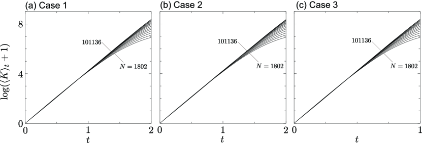
Figure 1: The average cardinality versus time in logarithmic scale for (a) Case 1, (b) Case 2, and (c) Case 3 [cf. Eq. (5.3)]. Note that the range of $t$ in panel (c) is different from those in panels (a) and (b). For each curve, the ensemble average over $M$ different simulations is taken in order to decrease noise. We set $N\epsilon^{2}=1$ and $L=1$, while $(N,M)=(1802,72)$, $(2402,54)$, $(3203,40)$, $(4271,30)$, $(5695,23)$, $(7593,17)$, $(10125,13$, $(13500,10)$, $(18000,8)$, $(24000,6)$, $(32000,4)$, $(42666,3)$, $(56888,3)$, $(75851,2)$, and $(101135,2)$.

Before stating the numerical results, it is necessary to mention the mean free time $\tau$ of the system. The mean free time $\tau$ at an equilibrium state (with energy $E$) can be easily computed as $\tau=[4(2\pi E/3)^{1/2}N\epsilon^{2}]^{-1}$, see [12]. Therefore, we obtain $\tau=(4\sqrt{\pi/3})^{-1}\approx 0.244$ for Cases 1 and 2, and $\tau=(8\sqrt{\pi/3})^{-1}\approx 0.122$ for Case 3. On the other hand, $\tau$ can be also computed from the numerical simulation. At the end of the simulation, we know $m_{c}$, which is the total number of collisions between particles. Since a single collision involves two particles, the total number of particles involved in $m_{c}$ collisions is $2m_{c}$. The time–averaged free time is then $t/(2m_{c})$, during which one of the $N$ particles experiences a collision with one of the others. Thus, for a tagged particle, it takes $Nt/(2m_{c})$ (on average) to experience a collision with one of the others. In the simulation, we have obtained $Nt/(2m_{c})=0.242$ for Case 1, $Nt/(2m_{c})=0.241$ for Case 2 and $Nt/(2m_{c})=0.121$ for Case 3 when $N=101135$ and $t=2$.

Table 1: The value of $\frac{1}{t}\log(\langle K\rangle_{t}+1)$

	Case 1			Case 2			Case 3
$t$ $\backslash$ $N$	$1802$	$10125$	$101135$	$1802$	$10125$	$101135$	$1802$	$10125$	$101135$
0.4	4.288	4.201	4.199	4.290	4.244	4.190	8.576	8.403	8.399
0.8	4.227	4.221	4.223	4.222	4.253	4.211	8.455	8.442	8.446
1.2	4.090	4.199	4.233	4.088	4.216	4.223	8.180	8.399	8.467
1.6	3.840	4.116	4.230	3.841	4.118	4.218	7.680	8.233	8.461
2.0	3.462	3.916	4.191	3.467	3.925	4.180	6.924	7.833	8.382

The plot in Fig. 1 and values in Table 1 show that the exponential behavior $\langle K\rangle_{t}\approx e^{rt}-1$ is approached as $N$ increases ($\varepsilon$ decreases), in a range of times including several mean free flights. The value of $\frac{1}{t}\log(\langle K\rangle_{t}+1)$, which should converge to $r$ as $N\to\infty$ and $t\to\infty$, in Case 1 and that in Case 2 are almost coincident, as expected from the discussion before Eq. (2.20). Observe that no transient is even visible in the case of a non–equilibrium, uniform distribution of velocities (Case 2). It is seen from Table 1 that the value of $\frac{1}{t}\log(\langle K\rangle_{t}+1)$ in Case 3 is almost twice larger than that of Case 1. This verifies (2.20) (here $\beta=3$ in Case 1 and $\beta=3/4$ in Case 3).

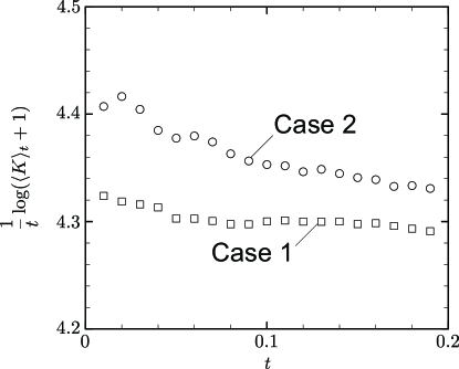
Figure 2: The value of $\frac{1}{t}\log(\langle K\rangle_{t}+1)$ for Cases 1 (square) and 2 (circle) in the range of time less than one mean free time; $(N,M)=(1802,720)$.

Finally, we have checked whether $r$ is different between Cases 1 and 2, especially for small time $t\in[0,0.2]$. Note that $t\in[0,0.2]$ is within one mean free time at equilibrium $(\tau\approx 0.244)$. Figure 2 shows that the values of $\frac{1}{t}\log(\langle K\rangle_{t}+1)$ for both cases differ, but the discrepancy is small.

Acknowledgments. The authors would like to thank Chiara Saffirio and Herbert Spohn for stimulating discussions. S. Simonella has been partially supported by PRIN 2009 Teorie cinetiche e applicazioni and by Indam COFUND Marie Curie fellowship 2012, call 10. T. Tsuji has been supported by the JSPS Institutional Program for Young Researcher Overseas Visits.

References

[1]
A. V. Bobylev. The theory of the nonlinear spatially uniform Boltzmann equation for
Maxwell molecules.
Soviet Sci. Rev. Sect. C Math. Phys. Rev.7, Harwood Academic Publ., Chur, 1988.
[2]
E. A. Carlen, M. C. Carvalho and E. Gabetta.
Central limit theorem for Maxwellian molecules and truncation of the Wild expansion.
Comm. Pure Appl. Math.53, 3, 370–397, 2000.
[3]
L. Desvillettes. Some applications of the method of moments for the homogeneous Boltzmann
equation. Arch. Rational Mech. Anal.123, 4, 387–395, 1993.
[4]
A. Gabrielov, V. Keilis-Borok, Ya. Sinai and I. Zaliapin.
Statistical Properties of the Cluster Dynamics of the Systems of Statistical Mechanics.
In: Boltzmann’s Legacy, ESI Lectures in Mathematics and Physics, EMS Publishing House,
203–216, 2008.
[5] H. Grad. On the kinetic theory of rarefied gases.
Comm. on Pure and App. Math.2, 4, 331–407, 1949.
[6] H. Grad. Principles of the kinetic theory of gases.
S. Flügge ed. Handbuch der Physik12, 205–294, 1958.
[7] O. E. Lanford. Time evolution of large classical systems. In “Dynamical systems, theory and applications”,
Lecture Notes in Physics, ed. J. Moser, 38, 1–111, Springer–Verlag, Berlin, 1975.
[8]
H. J. McKean. Speed of approach to equilibrium for Kac s caricature of a Maxwellian gas. Arch.
Rational Mech. Anal.21, 343–367, 1966.
[9]
S. Mischler and B. Wennberg.
On the spatially homogeneous Boltzmann equation.
Ann. Inst. H. Poincaré Anal. Non Linéaire16, 4, 467–501, 1999.
[10]
M. Pulvirenti and S. Simonella. The Boltzmann–Grad limit of a hard sphere system:
analysis of the correlation error. Preprint, arXiv:1405.4676, 2014.
[11]
A. Pulvirenti and B. Wennberg. A Maxwellian lower bound for solutions to the Boltzmann
equation. Comm. Math. Phys.183, 145–160, 1997.
[12]
Y. Sone. Molecular Gas Dynamics: Theory, Techniques, and Applications.
Modeling and Simulation in Science, Engineering and Technology,
Springer Science & Business Media, 2007.
[13]
Ya.G. Sinai. Construction of Dynamics in Infinite Systems of Particles.
Theoretical and Mathematical Physics, 12, 487, 1973.
[14]
Ya.G. Sinai. Construction of Cluster Dynamics for Dynamical Systems of Statistical Mechanics.
Proc. of Moscow State University, N1, 152, 1974.
[15]
C. Villani. A review of mathematical topics in collisional kinetic theory.
Handbook of mathematical fluid dynamics, Vol. I, 71–305,
North–Holland, Amsterdam, 2002.
[16]
E. Wild. On Boltzmann equation in the kinetic theory of gases. Math. Proc. Cambridge Philos. Soc.47,
602–609, 1951.