Singularity formation for the compressible Euler equations

Abstract.

It is well-known that singularity will develop in finite time for hyperbolic conservation laws from initial nonlinear compression no matter how small and smooth the data are. Classical results, including Lax [14], John [13], Liu [22], Li-Zhou-Kong [16], confirm that when initial data are small smooth perturbations near constant states, blowup in gradient of solutions occurs in finite time if initial data contain any compression in some truly nonlinear characteristic field, under some structural conditions. A natural question is that: Will this picture keep true for large data problem of physical systems such as compressible Euler equations? One of the key issues is how to find an effective way to obtain sharp enough control on density lower bound, which is known to decay to zero as time goes to infinity for certain class of solutions. In this paper, we offer a simple way to characterize the decay of density lower bound in time, and therefore successfully classify the questions on singularity formation in compressible Euler equations. For isentropic flow, we offer a complete picture on the finite time singularity formation from smooth initial data away from vacuum, which is consistent with the small data theory. For adiabatic flow, we show a striking observation that initial weak compressions do not necessarily develop singularity in finite time. Furthermore, we follow [7] to introduce the critical strength of nonlinear compression, and prove that if the compression is stronger than this critical value, then singularity develops in finite time, and otherwise there are a class of initial data admitting global smooth solutions with maximum strength of compression equals to this critical value.

1. Introduction

The compressible Euler equations are the oldest system of nonlinear PDEs modeling the motion of gases. Under Lagrangian coordinates, the compressible Euler equations in one space dimension take the following form

$$\tau_{t}-u_{x} =0\,,$$ (1.1)

$$u_{t}+p_{x} =0\,,$$ (1.2)

$$\Big{(}\frac{1}{2}u^{2}+\mathcal{E}\Big{)}_{t}+(u\,p)_{x} =0\,,$$ (1.3)

where $x$ is the Lagrangian spatial variable, $t\in\mathbb{R}^{+}$ is the time. $\tau=\rho^{-1}$ denotes the specific volume for the density $\rho$. $p$, $u$ and $\mathcal{E}$ stand for the pressure, the velocity, and the specific internal energy, respectively. For polytropic ideal gases, it holds that

$$p=K\,e^{\frac{S}{c_{v}}}\,\tau^{-\gamma},\ \ \mathcal{E}=\frac{p\tau}{\gamma-1}\,,\ \ \gamma>1\,,$$ (1.4)

where $S$ is the entropy, $K$ and $c_{v}$ are positive constants, see [9] or [30]. For most gases, the adiabatic exponent $\gamma$ lies between $1$ and $3$, that is $1<\gamma<3$.

For $C^{1}$ solutions, it follows that (1.3) is equivalent to the “entropy equation”:

$$S_{t}=0\,.$$ (1.5)

Therefore, when entropy is constant, the flow is called isentropic, then (1.1) and (1.2) become a closed system, known as the $p$-system (or isentropic Euler equations)

$$\tau_{t}-u_{x} =0\,,$$ (1.6)

$$u_{t}+p_{x} =0\,,$$ (1.7)

with

$$p=K_{1}\,\tau^{-\gamma}\,,$$ (1.8)

where, $K_{1}>0$ is a constant.

Compressible Euler equations (1.1)–(1.3) and p-system (1.6)–(1.7) are two of the most important physical models for hyperbolic conservations laws

$${\bf u}_{t}+{\bf f}({\bf u})_{x}=0\,,$$ (1.9)

where ${\bf u}={\bf u}(x,t)\in\mathbb{R}^{n}$ is the unknown vector and ${\bf f}:\mathbb{R}^{n}\rightarrow\mathbb{R}^{n}$ is the nonlinear flux. It is a general belief that system (1.9) typically develops discontinuity singularity, i.e. shock wave, no matter how small and smooth the initial data are. This belief has been justified in a series of beautiful works by Lax [14] in 1964 for general systems with two unknowns, and by [13, 16, 17, 22] for general $n\times n$ systems. These results confirm that for general strictly hyperbolic systems, if the initial datum is a generic small smooth perturbation near a constant equilibrium, then the initial compression (negative spatial derivatives of gradient variables) in any truly nonlinear (not weakly linearly degenerate [16]) characteristic field develops singularity in finite time. Such lack of regularity is the major difficulty in analyzing these systems. With enormous efforts, the well-posedness theories of small total variation solutions for (1.9) including compressible Euler equations and p-system are fairly well understood [1, 10, 12]. The next natural question is on the theory of large data, which is, however, widely open. Even for some important physical systems, such as compressible Euler equations and p-system, the basic question, like if singularity will form in finite time, is not completely understood when the smallness condition on the initial data is missing. We will address this open problem in this paper for p-system and full compressible Euler equations.

The beautiful result of Lax [14] along with some expositions such as [11] left readers an impression that, at least for p-system, for $C^{1}$ initial data away from vacuum, singularity will form in finite time if and only if there is some compression (negative spatial derivatives of gradient variables, we refer the readers to Remark 2.4 below for the definition) initially, without smallness assumption. This, however, is not quite accurate. When adopting [14] to p-system, the control on a crucial term $\frac{1}{c(v)}$ for the sound speed $c(v)=\sqrt{-p_{v}}$ is very important. This term is singular if density tends to zero. On the other hand, the $L^{\infty}$ estimate through Riemann invariants offers an upper bound of density, without control on the lower bound. In the case of small solutions, one can actually choose the smallness of the perturbation carefully, so that the perturbation remains small comparing to the positive lower bound of initial density uniformly in time. Such choice of smallness gives a positive constant lower bound (say one half of the lower bound of initial density) for density. However, when initial data are large, this becomes a serious issue. In general, it is not possible to have a positive constant lower bound for density. Indeed, a Riemann problem connecting two extreme sides of two interacting strong rarefaction waves generates vacuum instantaneously when $t>0$, [30]. Smoothing out this data implies the existence of a $C^{1}$-solution such that $\inf_{x}\rho(x,t)\rightarrow 0$ as $t\rightarrow+\infty$. An example of Lipschitz continuous solutions can be found in the Section 82 in [9] using a method originally discussed in [28], where the density decays in time at a rate of $\frac{O(1)}{1+t}$. If one looks into this problem more carefully, the argument in [14] is valid only for p-system with large initial data and with pressure law (1.8) when $\gamma\geq 3$, which does not include the most practical case $1<\gamma<3$ in gas dynamics. In fact, when $\gamma\geq 3$, the control of lower bound of density is not needed, see also a generalization to full Euler equations by Chen, Young and Zhang [7]. Therefore, the real matter of the open problem is to establish the finite time singularity formation for both p-system and full compressible Euler equations for the most physical case $1<\gamma<3$. A more in-depth discussion on Lax’s result [14] will be presented in section 2 of this paper.

The main purpose of this paper is to establish the finite time singularity formation result for both p-system and full Euler equations without the smallness assumption on initial data, when gases are in physical regime, i.e., $1<\gamma<3$. We introduce a brand new elementary and neat approach to establish the time-dependent density lower bound, which is good enough to achieve our characteristic analysis leading to the finite time singularity formation results even when initial data are large.

For isentropic flow with $\gamma$-law pressure, our result shows that if the initial datum is smooth with a positive lower bound for density, then the classical solution of the Cauchy problem of p-system breaks down in finite time if and only if there is an initial compression. The precise statement is in Theorem 2.3, and the definitions of rarefaction and compression are given in Remark 2.4. We emphasize that the approach introduced in the proof of this theorem is neat and elementary, but also very powerful. The key new estimates are given by Lemmas 2.5 and 2.6. Note the time dependent lower bound we proved for density is not in the optimal order, but it is good enough for the singularity formation problem. Furthermore, this approach is applicable to the full Euler equations for non-isentropic flows.

We now make a brief remark on the time-dependent lower bound for density. In many literatures, using Eulerian formulation, and mass equation, the following estimate of density

$$\inf_{x}\rho_{0}(x)\exp\{-\int_{0}^{t}\|u_{x^{\prime}}(\cdot,\sigma)\|_{L^{\infty}}\ d\sigma\}\leq\rho(x,t),$$

has been obtained for $x^{\prime}$ the Eulerian space variable, c.f. [15]. We note that, since there is a possibility that the blowup of gradient of $u$ and the vanishing of density may happen at the same time, it is very difficult to use this estimate in the argument of proving global regularity or singularity formation. When initial data are purely rarefactive (see Remark 2.4 below for definition), L. Lin [18] proved that the density of any Lipschitz solution of p-system has a positive lower bound of order $\frac{1}{1+t}$ through a relatively complicated approximation generated by a polygonal scheme. This result, however, does not apply to the case when initial data contain compression, which is the mechanism for singularity formation. One of the main contributions of this paper is to provide a good enough new time-dependent estimate on the density lower bound for generic $C^{1}$ initial data away from vacuum, when $1<\gamma<3$. The idea we developed here is simple and neat, but does not offer the optimal rate $\frac{1}{1+t}$, which is achieved through a much more complicated method in our preprint [4] for generic $C^{1}$ initial data away from vacuum.

From the discussion above, we see that for isentropic flow, the singularity formation theory is not different no matter the data is small or large. One may thus expect a similar picture for the non-isentropic flow. However, the life is very complicated for non-isentropic flow. When initial data are small, under a so-called nonlinear wave condition, [16, 17, 22] showed that if the initial datum is a generic small smooth perturbation near a constant equilibrium, then the initial compression in any truly nonlinear (not weakly linearly degenerate [16]) characteristic field develops singularity in finite time, like in the p-system. When initial data are large, this expectation is not true for full Euler equations. In Section 3.5, we will provide an explicit example showing that for certain class of non-trivial initial data, which might be even periodic in space variable with non-zero derivatives, global classical solutions exist. This is in a sharp contrast to the isentropic case, where the non-trivial periodic initial data lead to finite time singularity formation of classical solutions. We remark that this class of initial data do not satisfy the so-called nonlinear wave condition in the blowup results of [22]. Therefore, in order to prove finite time singularity formation results for full Euler equations with large data, it is natural to impose some conditions to exclude this class of initial data, see also some related discussion in [7]. In Section 3, we will identify such kind of conditions and successfully establish the finite time singularity formation results when initial compression is merely stronger than a critical value, which can be attained by the global classical solutions constructed in our example. More detailed discussion will also be provided at the end of this paper. For full Euler system, singularity formation results were proved in [2, 7] for $\gamma\geq 3$ when the density lower bound is not needed, and for $1<\gamma<3$ with the help of an a priori assumption on the density lower bound. For small solutions, similar to isentropic case, smallness conditions give a positive constant lower bound for density, say one half of initial density lower bound. For large solutions, sufficiently good time-dependent density lower bound estimate is needed for the proof of finite time singularity formation, when $1<\gamma<3$. Our idea introduced for isentropic case can be generalized to full Euler system, and gives a good enough estimate on density lower bound. The singularity formation for p-system with general pressure law is discussed in the appendix.

When some restrictions, such as compactness of support of the initial data near certain constant equilibrium, are imposed, there are some wonderful results on the finite time singularity formation for compressible Euler equations in higher space dimensions. We refer the readers to some of these results, see [24, 27, 29] for classical compressible Euler equations, and see [8, 26] for relativistic Euler equations. The results in this paper in one space dimension offer more complete and clear pictures on the mechanism, occurrence, and the type of singularity formations.

2. Singularity formation for p-system

In this section, we study singularity formation for p-system (1.6)$\sim$(1.8). The proof of our main theorem (Theorem 2.3) is based on the study of Lax’s characteristic decomposition established first for general hyperbolic system with two unknowns in [14]. For the readers’ convenience, in Subsection 2.1, we first review this well-known result of Lax [14]. Then in Subsection 2.2, we present a careful adoption of Lax’s method in [14] to p-system with $\gamma$-law pressure. We will then explain why Lax’s result [14] for small smooth initial data for general $2\times 2$ system actually offers the singularity formation result for p-system without smallness restrictions on initial data for $\gamma$-law pressure provided that $\gamma\geq 3$. We will also spell out why his result does not include the most physical cases when $1<\gamma<3$. In the latter case, a careful study on the lower bound of density is needed, which is achieved in Subsection 2.3, leading to the first main result of this paper Theorem 2.3.

2.1. Lax’s result for $2\times 2$ systems

This part is basically taken from Lax’s paper [14] in 1964. Consider a system of two first-order partial differential equations

$$\begin{split}u_{t}+f_{x}=0\,,\\ v_{t}+g_{x}=0\,,\end{split}$$ (2.1)

where $f$ and $g$ are functions of $u$ and $v$. Carrying out the differentiation in (2.1), we obtain

$${\bf u}_{t}+A\,{\bf u}_{x}=0\,,$$ (2.2)

where

$${\bf u}=\left(\begin{array}[]{l}u\\ v\end{array}\right)\qquad\text{and}\qquad A=\left(\begin{array}[]{lr}f_{u}&f_{v}\\ g_{u}&g_{v}\end{array}\right)\,.$$

Suppose that this system is strictly hyperbolic, i.e. the matrix $A$ has real and distinct eigenvalues $\lambda<\mu$ for relevant values of $u$ and $v$. Use ${\bf l}_{\lambda}$ and ${\bf l}_{\mu}$ to denote the left eigenvectors of $A$ corresponding to eigenvalues $\lambda$ and $\mu$, respectively.

Multiplying (2.2) by ${\bf l}_{\lambda}$ and ${\bf l}_{\mu}$ respectively, we have

$${\bf l}_{\lambda}\cdot{\bf u}^{\prime}=0\,,\qquad{\bf l}_{\mu}\cdot{\bf u}^{\backprime}=0\,,$$

where we denote

$$\prime=\partial_{t}+\lambda\partial_{x}\,,\qquad\backprime=\partial_{t}+\mu\partial_{x}\,.$$

Suppose there exist integrating factors $\phi$ and $\psi$ such that $\phi{\bf I}_{\lambda}=\nabla_{(u,v)}w(u,v)$, and $\psi{\bf I}_{\mu}=\nabla_{(u,v)}z(u,v)$, and therefore

$$w^{\prime}=\phi_{\lambda}\,{\bf l}_{\lambda}\cdot{\bf u}^{\prime}=0,\,\ z^{\backprime}=0.$$ (2.3)

for some functions $w(u,v)$ and $z(u,v)$, which are called Riemann invariants along characteristics with characteristic speeds $\lambda$ and $\mu$, respectively. Therefore, the $L^{\infty}$ norms on $w$ and $z$ are bounded by the initial data. We remark that such $\phi$ and $\psi$ always exist at least locally. Thus, for general hyperbolic systems with two unknowns, there always exist two Riemann invariants for different families, if we restrict the initial data to be a small perturbation near a constant equilibrium. This is also one of the reasons that Lax’s result in [14] is a small data theory. For many general systems, such as p-system, Riemann invariants are naturally well-defined globally, therefore, the smallness restriction is not an issue for this step.

We focus on $w$, the case on $z$ can be treated in a similar manner. Differentiating $w^{\prime}=0$ in (2.3) on $x$, we have

$$w_{tx}+\lambda w_{xx}+\lambda_{w}w_{x}^{2}+\lambda_{z}w_{x}z_{x}=0\,.$$ (2.4)

Also by (2.3), we observe from

$$0=z^{\backprime}=z^{\prime}-(\lambda-\mu)z_{x}\,,$$

that

$$z_{x}=\frac{z^{\prime}}{\lambda-\mu}\,.$$ (2.5)

Substituting (2.5) into (2.4) and denoting

$$\alpha:=w_{x}\,,$$

one finds

$$\alpha^{\prime}+\lambda_{w}\alpha^{2}+\frac{\lambda_{z}}{\lambda-\mu}z^{\prime}\alpha=0\,.$$ (2.6)

Let $h$ be a function of $w$ and $z$ satisfying

$$h_{z}=\frac{\lambda_{z}}{\lambda-\mu}\,.$$

Using $w^{\prime}=0$ in (2.3), we have

$$h^{\prime}=h_{w}w^{\prime}+h_{z}z^{\prime}=\frac{\lambda_{z}}{\lambda-\mu}z^{\prime}\,.$$

This, together with (2.6), gives

$$\alpha^{\prime}+\lambda_{w}\alpha^{2}+h^{\prime}\alpha=0\,.$$ (2.7)

Multiplying (2.7) by $e^{h}$ and denoting

$$\widetilde{\alpha}:=e^{h}\alpha\,,$$

we finally obtain

$$\widetilde{\alpha}^{\prime}=-a{\widetilde{\alpha}}^{2}\,$$ (2.8)

with

$$a:=e^{-h}\lambda_{w}\,.$$

This Riccati type equation gives us a clear passage to study the singularity formation and/or global existence of classical solutions for hyperbolic system with two unknowns. In fact, we could formally solve gradient variable $\widetilde{\alpha}$ along a characteristic $x(t)$ defined by

$$\frac{dx(t)}{dt}=\lambda,\ x(0)=x_{0},$$

to obtain

$$\frac{1}{\widetilde{\alpha}(x(t),t)}=\frac{1}{\widetilde{\alpha}(x_{0},0)}+\int_{0}^{t}a(x(\sigma),\sigma)~{}d\sigma$$

where the integral is taken along the characteristic curve $x(t)$.

Note that $a\neq 0$ if $\lambda_{w}\neq 0$, which is corresponding to the nonlinearity of the system. One does not expect singularity formation for linearly degenerate fields [22]. For simplicity, suppose that $a$ is always non-zero, which is also satisfied by the solution of p-system if initially $a\neq 0$. To fix the idea, we only consider the case $a>0$. If $\widetilde{\alpha}(0)<0$, i.e. initial solution is compressive somewhere in the $\lambda$ direction, then $\widetilde{\alpha}(t)$ breaks down if there exists a time $t_{*}>0$ such that

$$\int_{0}^{t_{*}}a(x(\sigma),\sigma)~{}d\sigma=-\frac{1}{\widetilde{\alpha}(x_{0},0)}\,.$$ (2.9)

which could be relaxed to

$$\int_{0}^{\infty}a(x(\sigma),\sigma)~{}d\sigma=\infty\,.$$ (2.10)

In [14], Lax considered the hyperbolic system with uniformly strict hyperbolicity, i.e. characteristic speeds $\lambda$ and $\mu$ are uniformly away from each other. With the help of smallness condition on initial data, there is a positive constant ${\bar{a}}$ such that $a\geq{\bar{a}}>0$, if the initial data are chosen so, hence (2.10) is automatically justified.

When smallness condition on the initial data is lacking, in principle, one expects the similar results following Lax [14] if the Riemann invariants are defined globally, and (2.10) is satisfied. For p-system (1.6)$\sim$(1.8), the Riemann invariants are defined globally, it remains to check (2.10). We will explain how far Lax’s theory can reach in the next subsection.

2.2. Lax’s large data theory on p-system: $\gamma\geq 3$.

We adopt Lax’s theory on singularity formation to the following Cauchy problem of p-system (1.6)$\sim$(1.8), i.e.,

$$\begin{cases}&\tau_{t}-u_{x}=0\,,\\ &u_{t}+p_{x}=0\,,\ p=K_{1}\,\tau^{-\gamma},\\ &\tau(x,0)=\tau_{0}(x),\ u(x,0)=u_{0}(x),\end{cases}$$ (2.11)

where, $K_{1}>0$ and $\gamma>1$ are constants. If the initial data are chosen to be a small smooth perturbation near a constant state $({\bar{\tau}},{\bar{u}})$ with ${\bar{\tau}}>0$, then Lax’s theory in [14] applied directly. Our main concern in this subsection is how far it could reach when initial data are not small.

From now on, we make the following assumption throughout the rest of Section 2:

Assumption 2.1.

Assume that $(\tau_{0}(x),u_{0}(x))$ are $C^{1}$ functions, and there are uniform positive constants $M_{1}$ and $M_{2}$ such that

$$\|(\tau_{0},u_{0})(x)\|_{C^{1}}\leq M_{1},\ \tau_{0}\geq M_{2}.$$

A direct calculation shows that (2.11) has two characteristic speeds

$$\lambda=-\mu=-c,$$

where $c$ is the Lagrangian sound speed

$$c:=\sqrt{-p_{\tau}}=\sqrt{K_{1}\,\gamma}\,{\tau}^{-\frac{\gamma+1}{2}}\,.$$ (2.12)

The forward and backward characteristics are defined by

$$\frac{dx^{+}}{dt}=c\quad{\textrm{and}}\quad\frac{dx^{-}}{dt}=-c\,,$$

respectively. We denote the corresponding directional derivatives along them by

$$\partial_{+}:=\textstyle{\frac{\partial}{\partial t}}+c\,\textstyle{\frac{\partial}{\partial x}}\quad{\textrm{and}}\quad\partial_{-}:=\textstyle{\frac{\partial}{\partial t}}-c\,\textstyle{\frac{\partial}{\partial x}}\,,$$

respectively. Furthermore, introducing the following useful quantity, c.f. [2],

$$\eta:=\int^{\infty}_{\tau}{c\,d\tau}=\textstyle\frac{2\sqrt{K_{1}\gamma}}{\gamma-1}\,\tau^{-\frac{\gamma-1}{2}}>0\,,$$ (2.13)

the globally defined Riemann invariants of (2.11) are

$$r:=u-\,\eta\quad{\textrm{and}}\quad s:=u+\,\eta\,,$$ (2.14)

which satisfy

$$\partial_{+}s=0\quad{\textrm{and}}\quad\partial_{-}r=0\,,$$ (2.15)

respectively.

Since $\eta$, $p$ and $c$ all are functions of $\tau$, their relations are as follows

$$\tau=K_{\tau}\,\eta^{-\frac{2}{\gamma-1}}\,,\quad p=K_{p}\,\eta^{\frac{2\gamma}{\gamma-1}}\,,\ \quad c=\sqrt{-p_{\tau}}=K_{c}\,\eta^{\frac{\gamma+1}{\gamma-1}}\,,$$ (2.16)

where $K_{\tau}$, $K_{p}$ and $K_{c}$ are positive constants given by

$$K_{\tau}:=\Big{(}\frac{2\sqrt{K_{1}\gamma}}{\gamma-1}\Big{)}^{\frac{2}{\gamma-1}}\,,\quad K_{p}:=K_{1}\,K_{\tau}^{-\gamma},\quad{\textrm{and}}\quad K_{c}:=\textstyle\sqrt{K_{1}\gamma}\,K_{\tau}^{-\frac{\gamma+1}{2}}\,.$$ (2.17)

Clearly, one has

$$K_{p}=\textstyle\frac{\gamma-1}{2\gamma}K_{c}\quad{\textrm{and}}\quad K_{\tau}K_{c}=\frac{\gamma-1}{2}\,.$$ (2.18)

In this paper, we always use $K$ with some subscripts to denote positive constants. We will not alert the readers again if there is no ambiguity.

We observe from (2.15) that the $L^{\infty}$ norm of $(r,s)$ are bounded by the initial data, which leads to a uniform $L^{\infty}$ bounds on $u$ and $\eta(\tau)$ with the help of (2.14). From (2.13), one finds the uniform positive lower bound on the specific volume $\tau$, or equivalently, the uniform upper bound on the density $\rho=\frac{1}{\tau}$. However, we remark that, such estimates do not offer any control on the lower bound of density $\rho$ (or, upper bound of $\tau$).

Following the procedure of last subsection in deriving (2.8), c.f. [2], the good gradient variables are

$$y:=\eta^{\frac{\gamma+1}{2(\gamma-1)}}\,s_{x}\quad{\textrm{and}}\quad q:=\eta^{\frac{\gamma+1}{2(\gamma-1)}}\,r_{x}\,,$$

which satisfy the following Riccati type equations:

$$\partial_{+}y =-a_{2}\,y^{2}\,,$$ (2.19)

$$\partial_{-}q =-a_{2}\,q^{2}\,,$$ (2.20)

where

$${a}_{2} :=K_{c}\,{\textstyle\frac{\gamma+1}{2(\gamma-1)}}\,\eta^{\frac{3-\gamma}{2(\gamma-1)}}\,.$$ (2.21)

We note the behavior of ${a}_{2}$ is purely determined by $\eta$. Since $\eta$ has a uniform upper bound, when $\gamma\geq 3$, there exists a uniform constant ${\bar{a}}_{2}>0$, such that $a_{2}\geq{\bar{a}}_{2}$. In this case (2.10) is justified, and Lax’s theory applies without smallness condition.

Proposition 2.2.

(A corollary from [14]) Assume that $(\tau_{0}(x),u_{0}(x))$ satisfy the conditions in Assumption 2.1. When $\gamma\geq 3$, classical solution of (2.11) breaks down if there is a point $x_{*}\in\mathbb{R}$ such that

$$s_{x}(x_{*},0)<0\quad{\textrm{or}}\quad r_{x}(x_{*},0)<0\,.$$ (2.22)

Proof.

We will show that if $s_{x}(x,0)<0$ or $r_{x}(x,0)<0$ for some $x$, then singularity forms in finite time. Without loss of generality, we assume that $s_{x}(x^{*},0)<0$, then $y(x^{*},0)<0$ for some $x^{*}$. Denote the forward characteristic passing $(x^{*},0)$ as $x^{+}(t)$. By (2.19),

$$\frac{1}{y(x^{+}(t),t)}=\frac{1}{y(x^{*},0)}+\int_{0}^{t}\,{a_{2}}(x^{+}(\sigma),\sigma)\;d\sigma\,,$$ (2.23)

where $a_{2}\geq{\bar{a}}_{2}$ for some uniform constant ${\bar{a}}_{2}>0$. Therefore, the right hand side of (2.23) approaches zero in finite time, which means singularity happens in finite time. ∎

However, for most physical gases where $1<\gamma<3$, the positive lower bound of the function ${a}_{2}$ requires positive lower bound of density. We remark that, for generic smooth initial data without initial vacuum, even for the global smooth solutions of (2.11), the density does not have constant positive lower bound in general. An example of Lipschitz continuous solutions can be found in [28] and some detailed discussion in Section 82 of [9], where the density decays in time at a rate of $\frac{1}{1+t}$. In view of (2.10), the lower bound of $a_{2}$ cannot decay too fast for possible singularity formation in finite time. Therefore, a new idea is needed to obtain a sufficiently sharp control on the time-dependent positive lower bound of density. This will be one of our main contributions in this paper, which will be addressed in the next subsection.

2.3. Singularity formation in p-system: $\gamma>1$

In this section, for all $\gamma>1$, we prove the singularity formation for the Cauchy problem in p-system when initial data contain some compression, and otherwise the global existence of smooth solutions. This is achieved by establishing a sharp enough time-dependent positive lower bound on density. The following theorem is the first main result of this paper.

Theorem 2.3.

For $\gamma>1$, if $(\tau_{0}(x),u_{0}(x))$ satisfy conditions in Assumption 2.1, then the Cauchy problem (2.11) has a unique global-in-time classical solution if and only if

$$s_{x}(x,0)\geq 0\quad{\textrm{and}}\quad r_{x}(x,0)\geq 0,\quad{\textrm{for all}}\quad x\in\mathbb{R}\,.$$ (2.24)

Remark 2.4.

At a point $(x,t)$, the solution of (2.11) is said to be forward rarefactive (resp. compressive) if $s_{x}(x,t)\geq 0$ (resp. $s_{x}(x,t)<0$); the solution is said to be backward rarefactive (resp. compressive) if $r_{x}(x,t)\geq 0$ (resp. $r_{x}(x,t)<0$).

Hence this theorem can be understood as that classical global-in-time solution of p-system exists if and only if the initial data are nowhere compressive.

If (2.24) is not satisfied at any point, that is, if the initial data contain some compression, then gradient blowup happens in finite time.

In order to prove Theorem 2.3, the following observation plays an important role. From (2.19) and (2.20), using comparison principle for ODEs, with the help of the following two non-negative constants $Y$ and $Q$ defined by

$$Y=\max\Big{\{}0,\ \sup_{x}\{y(x,0)\}\Big{\}},\quad Q=\max\Big{\{}0,\ \sup_{x}\{q(x,0)\}\Big{\}},$$ (2.25)

it is easy to see the following lemma holds.

Lemma 2.5.

If $(\tau_{0}(x),u_{0}(x))$ satisfy Assumption 2.1, it holds for $C^{1}$ solution $(\tau,u)(x,t)$ of (2.11) that

$$y(x,t)\leq Y,\quad\text{and}\quad q(x,t)\leq Q\,.$$

With the help of this Lemma 2.5, we are able to prove the following key estimate on the lower bound of density (equivalently, upper bound of $\tau$), for $1<\gamma<3$, covering most physical cases for polytropic gases.

Lemma 2.6.

Let $(\tau,u)(x,t)$ be a $C^{1}$ solution of (2.11) defined on time interval $[0,T]$ for some $T>0$, with initial data $(\tau_{0}(x),u_{0}(x))$ satisfying conditions in Assumption 2.1. If $1<\gamma<3$, then for any $x\in\mathbb{R}$ and $t\in[0,T)$, there is a positive constant $K_{0}$ depending only on $\gamma$, such that

$$\tau(x,t)\leq\big{[}{\tau_{0}}^{\frac{3-\gamma}{4}}(x)+K_{0}(Y+Q)t\big{]}^{\frac{4}{3-\gamma}}.$$

Proof.

From the definition of $y$ and $q$, it is clear that

$$y=s_{x}\sqrt{\frac{c}{K_{c}}},\ \quad q=r_{x}\sqrt{\frac{c}{K_{c}}},$$

which implies that

$$(y+q)=\sqrt{\frac{c}{K_{c}}}(r_{x}+s_{x})=2u_{x}\sqrt{\frac{c}{K_{c}}}.$$

Therefore, we read from the mass equation that

$$\sqrt{c}\,\tau_{t}=\frac{1}{2}\sqrt{K_{c}}(y+q).$$

Using the formula of sound speed (2.12), Lemma 2.5, one finds

$$\tau^{-\frac{\gamma+1}{4}}\tau_{t}\leq\frac{1}{2}(K_{1}\gamma)^{-\frac{1}{4}}\sqrt{K_{c}}(Y+Q).$$ (2.26)

When $1<\gamma<3$, $\frac{\gamma+1}{4}<1$, then for any $x\in\mathbb{R}$, and $t\in[0,T)$, a simple time integration shows that

$$\tau(x,t)\leq\big{[}{\tau_{0}}^{\frac{3-\gamma}{4}}(x)+K_{0}(Y+Q)t\big{]}^{\frac{4}{3-\gamma}},$$

where $K_{0}=\frac{3-\gamma}{8}(K_{1}\gamma)^{-\frac{1}{4}}\sqrt{K_{c}}$. This completes the proof of this lemma. ∎

Remark 2.7.

We remark that, for purely rarefactive initial data, i.e. the initial data satisfying the conditions of Assumption 2.1 and (2.24), Lin [18] proved that the density of any Lipschitz solution of (2.11) has a positive lower bound of order $\frac{1}{1+t}$ through a relatively complicated approximation generated by a polygonal scheme. This Lemma 2.6 works for general data as long as $\gamma\in(1,3)$. Although the time-dependent bound is not as sharp as that in [18], the proof is much simpler and elementary. A generalization of [18] with $\frac{O(1)}{1+t}$ bound on density to general initial data for all $\gamma>1$ has been carried out in our work [4]. This $\frac{O(1)}{1+t}$ rate is optimal for generic $C^{1}$ initial data due to the example in [9, 28].

We now give a proof for Theorem 2.3.

Proof of Theorem 2.3.

1) Sufficiency. In this part, we prove that under Assumption 2.1, if the initial data satisfy the condition (2.24), then problem (2.11) admits a unique global $C^{1}$ solution. As a matter of fact, this is a direct consequence of the result presented in [18]. We give an outline here.

Recall that the local-in-time existence of $C^{1}$ solutions for (2.11) can be proved by classical method, c.f. Theorem 4.1 on page 66 of [32], see also [15, 10], where the life-span of classical solution depends on the $C^{1}$-norm of the initial data and the positive lower bound of $\tau_{0}$. The main idea is to use the standard continuity argument to extend the local classical solutions to global with a priori estimates in $L^{\infty}$ and Lipschitz norms of $(\tau,u)(x,t)$. Indeed, the uniform $L^{\infty}$ bounds of $u(x,t)$ and the lower bound of $\tau(x,t)$ follow from those of $(r,s)(x,t)$ which are constant along their characteristics, respectively; see (2.15). For Lipschitz norms, we know from (2.24), that $y(x,0)\geq 0$ and $q(x,0)\geq 0$, and thus $\|y(x,t)\|_{L^{\infty}}\leq Y$, and $\|q(x,t)\|_{L^{\infty}}\leq Q$. Now, the result of [18] offers that, for initial data satisfying Assumption 2.1 and (2.24), for any Lipschitz continuous solutions of (2.11), there is a positive constant ${\bar{K}}_{0}$, independent of time, such that

$$\tau\leq{\bar{K}}_{0}(1+t),$$

which gives the upper bound of $\tau(x,t)$. Furthermore, we deduce from the definitions of $y$, $q$, and $\eta$ that, there exists a function ${\widetilde{C}}(t)$ satisfying $1\leq{\widetilde{C}}(t)<\infty$ for any positive finite time $t$ that

$$\|(r_{x},s_{x},\tau_{x},u_{x})(x,t)\|_{L^{\infty}}\leq{\widetilde{C}}(t).$$

Now, if the maximal existence time $T_{*}$ of $C^{1}$ solution is finite, then ${\widetilde{C}}({T_{*}})$ is finite, so are $L^{\infty}$ norm of $(\tau,u)(x,T_{*})$. One can then apply these estimates and the local existence result to show there exists a positive time ${\bar{t}}$ such that the $C^{1}$ solution can be further extended to the time interval $[0,T_{*}+{\bar{t}})$ contradicting the fact that $T_{*}$ is maximal. Therefore, $T_{*}=\infty$.

2) Necessity. In this part, we shall prove that under Assumption 2.1, if the initial data fail to satisfy the condition (2.24) at one point ${x^{*}}\in\mathbb{R}$, the $C^{1}$ solution of (2.11) must blow up in its derivatives in finite time. Without loss of generality, we assume that $s_{x}(x^{*},0)<0$, then $y(x^{*},0)<0$. When $\gamma\geq 3$, this was shown in the last section. Here, we only have to consider the case $1<\gamma<3$, in which ${a}_{2}$ vanishes when density goes to zero. We denote the forward characteristic passing $(x^{*},0)$ as $x^{+}(t)$. In view of (2.23),

$$\frac{1}{y(x^{+}(t),t)}=\frac{1}{y(x^{*},0)}+\int_{0}^{t}\,{a_{2}}(x^{+}(\sigma),\sigma)\;d\sigma\,.$$

To show $y$ blows up in finite time, it is enough to show that

$$\int_{0}^{\infty}\,{a_{2}(x^{+}(t),t)}\;dt=\infty\,,$$

where the integral is along characteristic $x^{+}(t)$. We read from Lemma 2.6, and the definition of $a_{2}$ that

$$a_{2}(x^{+}(t),t)\geq\frac{\gamma+1}{4}K_{\tau}^{-\frac{\gamma+1}{4}}\big{[}M_{1}^{\frac{3-\gamma}{4}}+K_{0}(Y+Q)t\big{]}^{-1}.$$

Hence,

$$\int_{0}^{\infty}\,{a_{2}(x^{+}(t),t)}\;dt=\infty\,.$$

Therefore, $y$ and $s_{x}$ blow up in finite time. The proof of the theorem is completed. ∎

Remark 2.8.

The method developed here can be applied to p-system with general pressure laws. Under some mild structural conditions, a similar result to Theorem 2.3 has been established in the section 2.4 of our preprint arXiv:1408.6775v2.

3. Full compressible Euler equations

In this section, we consider the following Cauchy problem of full compressible Euler equations

$$\begin{cases}\tau_{t}-u_{x}=0\,,\\ u_{t}+p_{x}=0\,,\ p=Ke^{\frac{S}{c_{v}}}\tau^{-\gamma},\ \gamma>1,\\ S_{t}=0\,,\\ (\tau,u,S)(x,0)=(\tau_{0},u_{0},S_{0})(x).\end{cases}$$ (3.1)

Here, we replaced the energy equation with entropy equation. For smooth solutions, we see that $S(x,t)=S_{0}(x):=S(x)$. Throughout this section, we require that the initial data $(\tau_{0},u_{0},S_{0})(x)$ satisfy conditions in the following assumption.

Assumption 3.1.

Assume that $(\tau_{0}(x),u_{0}(x))\in C^{1}(\mathbb{R})$, $S_{0}(x)\in C^{2}(\mathbb{R})$, and there are uniform positive constants $M_{1}$ and $M_{2}$ such that

$$\|(\tau_{0},u_{0})(x)\|_{C^{1}}+\|S_{0}(x)\|_{C^{2}}\leq M_{1},\ \tau_{0}\geq M_{2}.$$

For smooth solutions, it is often convenient to choose some new variables. Define

$$m:=e^{\frac{S}{2c_{v}}}>0,\quad c:=\sqrt{-p_{\tau}}=\sqrt{K\,\gamma}\,{\tau}^{-\frac{\gamma+1}{2}}\,e^{\frac{S}{2c_{v}}}\,,$$ (3.2)

and

$$\eta:=\int^{\infty}_{\tau}{\frac{c}{m}\,d\tau}=\textstyle\frac{2\sqrt{K\gamma}}{\gamma-1}\,\tau^{-\frac{\gamma-1}{2}}>0\,,$$ (3.3)

where $c$ is the nonlinear Lagrangian sound speed. Direct calculations show that (c.f. [2, 7])

$$\tau =K_{\tau}\,\eta^{-\frac{2}{\gamma-1}}\,,$$

$$p =K_{p}\,m^{2}\,\eta^{\frac{2\gamma}{\gamma-1}}\,,$$ (3.4)

$$c =c(\eta,m)=K_{c}\,m\,\eta^{\frac{\gamma+1}{\gamma-1}}\,.$$

We remark that, we still use $\eta$, $c$, and many other functions appeared in Section 2 for full Euler equations. These functions are natural extensions from isentropic flows to adiabatic ones, in the sense that they are different to each other only by a positive constant multiple when $S$ is chosen as a constant.

For $C^{1}$ solutions, the problem (3.1) is equivalent to (c.f. [10, 30])

$$\begin{cases}\eta_{t}+\frac{c}{m}\,u_{x}=0\,,\\ u_{t}+m\,c\,\eta_{x}+2\frac{p}{m}\,m_{x}=0\,,\\ m_{t}=0\,,\\ (\eta,u,m)(x,0)=(\eta_{0},u_{0},m_{0})(x)=(\eta(\tau_{0}(x)),u_{0}(x),m(S_{0}(x))).\end{cases}$$ (3.5)

Due to the linear degeneracy, in the regime of smooth solutions, $m$ is independent of time, we thus fix $m=m(x)=m_{0}(x)$ in the rest of this paper. Therefore, formally, one can still treat (3.5) as a system of two (significant) equations, with fluxes (pressure) depending on $x$ explicitly. Like in the case of isentropic flows, two truly nonlinear characteristic fields are

$$\frac{dx^{+}}{dt}=c\quad{\textrm{and}}\quad\frac{dx^{-}}{dt}=-c\,,$$ (3.6)

and we denote the corresponding directional derivatives along these by

$$\partial_{+}:=\textstyle{\frac{\partial}{\partial t}}+c\,\textstyle{\frac{\partial}{\partial x}}\quad{\textrm{and}}\quad\partial_{-}:=\textstyle{\frac{\partial}{\partial t}}-c\,\textstyle{\frac{\partial}{\partial x}}\,,$$

respectively. Comparing with p-system, one of significant differences for full Euler system is the disappearance of Riemann invariances, in fact, the Riemann variables are

$$r:=u-m\,\eta\,,\qquad s:=u+m\,\eta\,.$$ (3.7)

which vary along characteristics

$$\partial_{+}s =\frac{1}{2\gamma}\,\frac{c\,m_{x}}{m}\,(s-r)\,,$$ (3.8)

$$\partial_{-}r =\frac{1}{2\gamma}\,\frac{c\,m_{x}}{m}\,(s-r)\,.$$ (3.9)

Therefore, without smallness assumption of the solutions, the first non-trivial question one encounters is how to achieve $L^{\infty}$ estimates on the solutions. We remark that this question is trivial for isentropic case since $r$ and $s$ are invariant along their characteristics. Fortunately, this question is answered recently by G. Chen, R. Young and Q. Zhang in [7] under the following additional condition:

Assumption 3.2.

Assume that the initial entropy $S_{0}(x)$ has finite total variation, so that

$$V:=\frac{1}{2c_{v}}\int_{-\infty}^{+\infty}|S^{\prime}(x)|\;dx=\int_{-\infty}^{+\infty}\frac{|m^{\prime}(x)|}{m(x)}\;dx<\infty\,,$$ (3.10)

From Assumption 3.1, it is clear that there are positive constants $M_{L}$, $M_{U}$, $M_{s}$ and $M_{r}$ such that

$$0<M_{L}<m(x)<M_{U}\,,\quad|s_{0}(x)|<M_{s},\ \quad|r_{0}(x)|<M_{r}\,.$$ (3.11)

For ${\overline{V}}=\frac{V}{2\gamma}$, we now define

$$N_{1} :=M_{s}+\overline{V}\,M_{r}+\overline{V}\,(\overline{V}\,M_{s}+{\overline{V}}^{2}\,M_{r})\,e^{{\overline{V}}^{2}},$$

$$N_{2} :=M_{r}+\overline{V}\,M_{s}+\overline{V}\,(\overline{V}\,M_{r}+{\overline{V}}^{2}\,M_{s})\,e^{{\overline{V}}^{2}}.$$

The following proposition is proved in [7] by a highly non-trivial characteristic method.

Proposition 3.3.

[7] Assume the initial data $(\tau_{0},u_{0},S_{0})(x)$ satisfy the conditions in Assumptions 3.1 and 3.2. If $(\tau(x,t),u(x,t),S(x))$ is a $C^{1}$ solution of (3.1) for $t\in[0,T)$ for some positive $T$, then it holds that

$$|s(x,t)|\leq N_{1}{M_{U}}^{\frac{1}{2\gamma}},\quad|r(x,t)|\leq N_{2}{M_{U}}^{\frac{1}{2\gamma}},$$ (3.12)

$$|u(x,t)|\leq\frac{N_{1}+N_{2}}{2}{M_{U}}^{\frac{1}{2\gamma}},\ \eta(x,t)\leq\frac{N_{1}+N_{2}}{2}{M_{L}}^{\frac{1}{2\gamma}-1}:=E_{U}.$$ (3.13)

Therefore, there are positive constants $M_{\rho}$ such that

$$\rho\leq M_{\rho},\quad\tau\geq\frac{1}{M_{\rho}}.$$ (3.14)

The second major obstacle appears in the equations of gradient variables. Like in p-system, following the wisdoms of many previous works, c.f. [2, 14, 21], a good choice is

$$y :=m^{-\frac{3(3-\gamma)}{2(3\gamma-1)}}\,\eta^{\frac{\gamma+1}{2(\gamma-1)}}\,(s_{x}-{\textstyle\frac{2}{3\gamma-1}}\,m_{x}\,\eta),$$

$$q :=m^{-\frac{3(3-\gamma)}{2(3\gamma-1)}}\,\eta^{\frac{\gamma+1}{2(\gamma-1)}}\,(r_{x}+{\textstyle\frac{2}{3\gamma-1}}\,m_{x}\,\eta)\,,$$ (3.15)

which satisfy

$$\partial_{+}y =a_{0}-a_{2}\,y^{2},$$

$$\partial_{-}q =a_{0}-a_{2}\,q^{2},$$ (3.16)

where

$${a}_{0} :={\textstyle\frac{K_{c}}{\gamma}}\,\big{[}{\textstyle\frac{\gamma-1}{3\gamma-1}}\,m\,m_{xx}-{\textstyle\frac{(3\gamma+1)(\gamma-1)}{(3\gamma-1)^{2}}}\,m_{x}^{2}\big{]}\,m^{-\frac{3(3-\gamma)}{2(3\gamma-1)}}\,\eta^{\frac{3(\gamma+1)}{2(\gamma-1)}+1},$$

$${a}_{2} :=K_{c}\,{\textstyle\frac{\gamma+1}{2(\gamma-1)}}\,m^{\frac{3(3-\gamma)}{2(3\gamma-1)}}\,\eta^{\frac{3-\gamma}{2(\gamma-1)}}.$$ (3.17)

Clearly, $a_{0}=0$ if $S_{0}(x)$ (thus $m(x)$) is a constant. For general adiabatic flows, $a_{0}$ is not constant zero. (3.16) are not in Riccati type, and these different ODE structures lead to different behaviors of solutions, this is more crucial when initial data are not small perturbation around a constant state. Indeed, the classical theory of [16, 17, 22] confirms that, when initial data are arbitrarily small near a constant sate away from vacuum, $y$ and/or $q$ blows up in finite time if there is some nonlinear compression (under their notations) at some point $x\in\mathbb{R}$, under a so-called nonlinear wave condition [22]. We also note that the choice of gradient variables in [16, 17, 22] is slightly different from our choices here. Our choices of $y$ and $q$ seem better for large solutions. From now on, we adapt the notions to call the initial data are compressive at $x$ if $y(x,0)<0$ or $q(x,0)<0$, and rarefactive at $x$ if $y(x,0)\geq 0$ or $q(x,0)\geq 0$. We first present an example to show that weak initial compression does not necessary develop finite time gradient blowup.

Example 3.4.

For any $C^{1}$ functions $S(x)$ and $\tau(x)>0$,

$$u=0,\quad S=S(x)\quad\text{and}\quad\tau=\tau(x)$$

is a global $C^{1}$ (stationary) solution of (3.1) if in the initial data $S$ and $\tau$ are chosen such that

$$p_{x}(\tau(x),S(x))=0.$$ (3.18)

Therefore, if we choose a smooth non-constant function $S(x)$, then choose

$$\tau(x)=K_{\tau,S}\ \exp\left\{\frac{S(x)}{\gamma c_{v}}\right\},$$ (3.19)

for any positive constant $K_{\tau,S}$, $(\tau(x),0,S(x))$ is a smooth stationary solution of (3.1). In particular, if one chooses $S(x)$ to be a non-constant periodic function, so is $\tau$, this gives a non-constant solution of (3.1) which is periodic in both space and time. In order to fulfill the condition in Assumption 3.2, a choice of $S(x)$ is $\frac{1}{x^{2}+1}$.

For such class of solutions $(\tau(x),0,S(x))$, a direct calculation shows

$$-q(x)=y(x)=\textstyle\frac{\gamma-1}{\gamma(3\gamma-1)}m_{x}m^{\frac{3(\gamma-3)}{2(3\gamma-1)}}\eta^{\frac{3\gamma-1}{2(\gamma-1)}}\,.$$ (3.20)

which is non-zero at point $x$ if $S^{\prime}(x)\neq 0$. Therefore, either $q(x)<0$ or $y(x)<0$, but no singularity forms in the solution.

Remark 3.5.

At first glance, it seems that this example contradicts to Liu’s result [22]. We remark that this class of stationary solutions does not satisfy the nonlinear wave condition in [22] for singularity formation, and therefore there is no contradiction.

This example shows that weak nonlinear compression in initial data does not necessarily lead to finite time singularity formation especially when data could be large, see also some related discussion in [7]. This motivates our search for a critical strength of the nonlinear compression which offers finite time gradient blowup, which will be carried out in the next two subsections. In particular, the Section 3.1 is for the case when initial entropy has finite total variation, c.f. Assumption 3.2; while the Section 3.2 contains results without this condition. In addition to these obstacles, like in the case of isentropic flows, we still need to further generalize our method in p-system to non-isentropic case to find a sharp enough time-dependent density lower bound.

3.1. Singularity formation: $\|S_{0}(x)\|_{BV}<\infty$

In this subsection, we assume that the initial data $(\tau_{0}(x),u_{0}(x),S_{0}(x))$ satisfy the conditions in Assumptions 3.1 and 3.2, so the estimates in Proposition 3.3 hold.

The structure of (3.16) leads us to study the ratio $\frac{a_{0}}{a_{2}}$ which dominates behaviors of solutions to (3.16). A direct calculation is carried out as follows

$${\frac{a_{0}}{a_{2}}}={{\textstyle\frac{2(\gamma-1)^{2}}{\gamma(\gamma+1)(3\gamma-1)}}\,\big{(}m\,m_{xx}-{\textstyle\frac{3\gamma+1}{3\gamma-1}}\,m_{x}^{2}\big{)}}\,\eta^{\frac{3\gamma-1}{(\gamma-1)}}\,m^{-\frac{3(3-\gamma)}{(3\gamma-1)}}.$$ (3.21)

We define

$$b(x)=S_{xx}-\frac{1}{c_{v}(3\gamma-1)}S_{x}^{2},$$ (3.22)

and it is easy to see that

$$m^{2}b(x)={2c_{v}}\big{(}m\,m_{xx}-{\textstyle\frac{3\gamma+1}{3\gamma-1}}\,m_{x}^{2}\big{)}.$$ (3.23)

Therefore, $b(x)$ has the same sign as $a_{0}$. Also, we note from the definition of $m$ that there is a positive constant $M_{3}$ such that

$$|m\,m_{xx}-{\textstyle\frac{3\gamma+1}{3\gamma-1}}\,m_{x}^{2}|\leq M_{3}.$$ (3.24)

If we define a positive constant $N$ by

$$N:=\begin{cases}\sqrt{\frac{2(\gamma-1)^{2}}{\gamma(\gamma+1)(3\gamma-1)}\,M_{3}}\ E_{U}^{\frac{3\gamma-1}{2(\gamma-1)}}\ M_{L}^{-\frac{3(3-\gamma)}{2(3\gamma-1)}},&1<\gamma<3\,,\\ \sqrt{\frac{2(\gamma-1)^{2}}{\gamma(\gamma+1)(3\gamma-1)}\,M_{3}}\,E_{U}^{\frac{3\gamma-1}{2(\gamma-1)}}\,M_{U}^{-\frac{3(3-\gamma)}{2(3\gamma-1)}},&\gamma\geq 3\,,\end{cases}$$ (3.25)

we see

$$\frac{a_{0}}{a_{2}}\leq N^{2}.$$ (3.26)

Remark 3.6.

We remark that $a_{2}$ is positive, while $a_{0}$ usually changes sign for physical flows. In fact, for physical initial conditions of non-constant $S(x)$, the case for $b\leq 0$ for all $x\in\mathbb{R}$ cannot happen. Actually, from the relation (3.23), one finds that $b\leq 0$ is equivalent to $m\,m_{xx}-{\textstyle\frac{3\gamma+1}{3\gamma-1}}m_{x}^{2}\leq 0$, which is equivalent to

$$\big{(}m^{-\frac{2}{3\gamma-1}}\big{)}_{xx}\geq 0.$$

Therefore, $m^{-\frac{2}{3\gamma-1}}$ is a convex function over $\mathbb{R}$ if $b\leq 0$ for all $x\in\mathbb{R}$. This contradicts the fact that $0<M_{L}\leq m(x)\leq M_{U}$. Similar argument shows that the case for $b\geq 0$ for all $x$ cannot happen either.

Like Lemma 2.5, we are able to find uniform upper bounds for $y$ and $q$. Since it is a little more complicated than Riccati equation, we can simply compare (3.16) with the following ones

$$\partial_{+}{\widetilde{y}}=a_{2}(N^{2}-{\widetilde{y}}^{2}),\ \quad\partial_{-}{\widetilde{q}}=a_{2}(N^{2}-{\widetilde{q}}^{2}).$$ (3.27)

Therefore, it is easy to see the following lemma.

Lemma 3.7.

If $(\tau_{0},u_{0},S_{0})(x)$ satisfy conditions in Assumptions 3.1 and 3.2, it holds for $C^{1}$ solution $(\tau(x,t),u(x,t),S(x))$ of (3.1) that

$$y(x,t)\leq\max\Big{\{}N,\ \sup_{x}\{y(x,0)\}\Big{\}}=:\bar{Y}\,,$$

$$q(x,t)\leq\max\Big{\{}N,\ \sup_{x}\{q(x,0)\}\Big{\}}=:\bar{Q}\,.$$

The following lemma contains density lower bound estimate.

Lemma 3.8.

Let $(\tau(x,t),u(x,t),S(x))$ be a $C^{1}$ solution of (3.1) defined on time interval $[0,T]$ for some $T>0$, with initial data $(\tau_{0}(x),u_{0}(x),S_{0}(x))$ satisfying conditions in Assumptions 3.1 and 3.2. If $1<\gamma<3$, then for any $x\in\mathbb{R}$ and $t\in[0,T)$, there is a positive constant $K_{6}$ depending only on $\gamma$ and $M_{U}$, such that

$$\tau(x,t)\leq\big{[}{\tau_{0}}^{\frac{3-\gamma}{4}}(x)+K_{6}({\bar{Y}}+{\bar{Q}})t\big{]}^{\frac{4}{3-\gamma}}.$$

Proof.

From the mass equation in (3.1), (3.7), and (3.15), it is clear that

$$\begin{split}\tau_{t}=u_{x}&=\frac{1}{2}(r_{x}+s_{x})\\ &=m^{\frac{3(3-\gamma)}{2(3\gamma-1)}}\,\eta^{-\frac{\gamma+1}{2(\gamma-1)}}(q+y)\\ &\leq M_{U}^{\frac{3(3-\gamma)}{2(3\gamma-1)}}\,\eta^{-\frac{\gamma+1}{2(\gamma-1)}}({\bar{Y}}+{\bar{Q}}),\end{split}$$ (3.28)

where we have used Lemma 3.7. With the help of (3.3), we thus have

$$\tau^{-\frac{\gamma+1}{4}}\tau_{t}\leq M_{U}^{\frac{3(3-\gamma)}{2(3\gamma-1)}}\,(\textstyle\frac{2\sqrt{K\gamma}}{\gamma-1})^{-\frac{\gamma+1}{2(\gamma-1)}}({\bar{Y}}+{\bar{Q}}),$$ (3.29)

which implies that

$$\tau(x,t)\leq\big{[}\tau_{0}(x)+K_{6}({\bar{Y}}+{\bar{Q}})t\big{]}^{\frac{4}{3-\gamma}},$$ (3.30)

where

$$K_{6}=\frac{3-\gamma}{4}M_{U}^{\frac{3(3-\gamma)}{2(3\gamma-1)}}\,(\textstyle\frac{2\sqrt{K\gamma}}{\gamma-1})^{-\frac{\gamma+1}{2(\gamma-1)}}.$$

∎

In the following theorem, we show that $N$ is a critical measurement for the strength of initial nonlinear compression, which leads to finite time gradient blowup of solutions.

Theorem 3.9.

For $\gamma>1$, if $(\tau_{0}(x),u_{0}(x),S_{0}(x))$ satisfy conditions in Assumption 3.1 and 3.2, and if for $N$ defined in (3.25), it holds that

$$\inf_{x}\;\Big{\{}\ y(x,0),\ q(x,0)\ \Big{\}}<-N\,,$$ (3.31)

then for the $C^{1}$ solutions $(\tau(x,t),u(x,t),S(x))$ of (3.1), $|u_{x}|$ and/or $|\tau_{x}|$ blows up in finite time.

Remark 3.10.

The case when $\gamma\geq 3$ was carried out in [7], where density lower bound is not needed. [7] also mentioned a similar result of this Theorem with the a priori assumption of a positive constant lower bound on density. See Theorem 2.4 of [7] for details.

Proof.

Suppose that (3.31) holds. Without loss of generality, we can assume that $\inf_{x}y(x,0)<-N$, the case when $\inf_{x}q(x,0)<-N$ is similar. Then there exist $\varepsilon>0$ and $x_{0}\in\mathbb{R}$ such that

$$y(x_{0},0)<-(1+\varepsilon)\,N\,.$$ (3.32)

We denote the forward characteristic passing $(x_{0},0)$ as $x^{+}(t)$. Along this characteristic $x^{+}(t)$, from the definition of $N$, we have for any $t\geq 0$ such that $x^{+}(t)$ is well-defined,

$$\partial_{+}y(x^{+}(t),t)=a_{2}(\frac{a_{0}}{a_{2}}-y^{2})<0,\quad{\textrm{and}}\quad y(x^{+}(t),t)\leq y(x_{0},0)<-(1+\varepsilon)\,N.$$

Therefore,

$$\frac{y^{2}(x^{+}(t),t)}{(1+\varepsilon)^{2}}>N^{2}\geq\frac{a_{0}}{a_{2}},$$

which implies that

$$\partial_{+}y(x^{+}(t),t)=a_{2}(\frac{a_{0}}{a_{2}}-y^{2}(x^{+}(t),t))<-{\textstyle\frac{\varepsilon(2+\varepsilon)}{(1+\varepsilon)^{2}}}\,a_{2}\,y^{2}(x^{+}(t),t)\,.$$

Integrating it in time, we get

$$\frac{1}{y(x^{+}(t),t))}\geq{\frac{1}{y(x_{0},0)}+{\textstyle\frac{\varepsilon(2+\varepsilon)}{(1+\varepsilon)^{2}}}\int_{0}^{t}{a_{2}}(x^{+}(\sigma),\sigma)\;d\sigma}\,,$$ (3.33)

where the integral is along the forward characteristic. To show $y$ blows up in finite time, it is enough to show that

$$\int_{0}^{\infty}\,{a_{2}(x^{+}(t),t)}\;dt=\infty\,.$$ (3.34)

When $\gamma\geq 3$, from the definition of $a_{2}$ in (3.17), we see that

$$a_{2}\geq K_{c}\,{\textstyle\frac{\gamma+1}{2(\gamma-1)}}\,M_{L}^{\frac{3(3-\gamma)}{2(3\gamma-1)}}\,E_{U}^{\frac{3-\gamma}{2(\gamma-1)}},$$

thus (3.34) follows.

When $1<\gamma<3$, we read from Lemma 3.8, and the definition of $a_{2}$ in (3.17) that

$$a_{2}(x^{+}(t),t)\geq K_{c}\,{\textstyle\frac{\gamma+1}{2(\gamma-1)}}\,M_{L}^{\frac{3(3-\gamma)}{2(3\gamma-1)}}(\textstyle\frac{2\sqrt{K\gamma}}{\gamma-1})^{\frac{3-\gamma}{2(\gamma-1)}}\big{[}M_{1}^{\frac{3-\gamma}{4}}+K_{6}({\bar{Y}}+{\bar{Q}})t\big{]}^{-1},$$

therefore, (3.34) also follows.

Therefore, for any $\gamma>1$, $y$ and $s_{x}$ blow up in finite time. The proof of the theorem is completed.

∎

3.2. Singularity formation for general entropy function

We remark that singularity formation in Euler equations is a local behavior. We will remove several global constraints on entropy functions imposed in last subsection to include physically interesting cases such as spatially periodic solutions. For this purpose, in this subsection, we only impose conditions in Assumption 3.1 for the initial data, but not Assumption 3.2.

Without Assumption 3.2, we do not have the global uniform $L^{\infty}$ estimates in Proposition 3.3. However, we note that this result is proved by characteristic method, we thus could follow the same argument as in [7] to establish a local version.

For this purpose, we fix two initial points $\alpha<\beta\in\mathbb{R}$, denote the forward characteristic starting from $(\alpha,0)$ by $x_{\alpha}^{+}(t)$ and the backward characteristic starting from $(\beta,0)$ by $x_{\beta}^{-}(t)$. Assume that $(\tau(x,t),u(x,t),S(x))$ is a $C^{1}$ solution of (3.1) on the time interval $[0,T_{1}]$ for some positive $T_{1}$. In the trapezoid showed in figure 2 below, the top edge $t=T\leq T_{1}$ can shrink into one point, if $x_{\alpha}^{+}(T)=x_{\beta}^{-}(T)$. We denote this trapezoid domain by $\Omega_{\alpha,\beta,T}$, which is determined by the initial interval $[\alpha,\beta]$, $x_{\alpha}^{+}(t)$, $x_{\beta}^{-}(t)$, and $t=T$.

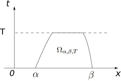
Figure 1. A domain of determination $\Omega_{\alpha,\beta,T}$

With the help of Assumption 3.1, on the interval $[\alpha,\beta]$, one has

$$V_{\alpha,\beta}:=\frac{1}{2c_{v}}\int_{\alpha}^{\beta}|S^{\prime}(\xi)|\;d\xi\leq\frac{1}{2c_{v}}M_{1}|\beta-\alpha|.$$ (3.35)

Therefore, if we define $\bar{V}_{\alpha,\beta}:=\frac{V_{\alpha,\beta}}{2\gamma}$, and

$${N_{1}}_{\alpha,\beta} :=M_{s}+\bar{V}_{\alpha,\beta}\,M_{r}+\bar{V}_{\alpha,\beta}\,(\bar{V}_{\alpha,\beta}\,M_{s}+{\bar{V}_{\alpha,\beta}}^{2}\,M_{r})\,e^{{\bar{V}_{\alpha,\beta}}^{2}},$$

$${N_{2}}_{\alpha,\beta} :=M_{r}+\bar{V}_{\alpha,\beta}\,M_{s}+\bar{V}_{\alpha,\beta}\,(\bar{V}_{\alpha,\beta}\,M_{r}+{\bar{V}_{\alpha,\beta}}^{2}\,M_{s})\,e^{{\bar{V}_{\alpha,\beta}}^{2}},$$

the same proof in [7] gives

Proposition 3.11.

Assume the initial data $(\tau_{0},u_{0},S_{0})(x)$ satisfy the conditions in Assumption 3.1. If $(\tau(x,t),u(x,t),S_{0}(x))$ is a $C^{1}$ solution of (3.1) for $t\in[0,T_{1})$ for some positive $T_{1}$, then it holds, for every point $(x,t)\in\Omega_{\alpha,\beta,T}$ and $T\leq T_{1}$, that

$$\begin{split}&|s(x,t)|\leq{N_{1}}_{\alpha,\beta}{M_{U}}^{\frac{1}{2\gamma}},\quad|r(x,t)|\leq{N_{2}}_{\alpha,\beta}{M_{U}}^{\frac{1}{2\gamma}}\\ &|u(x,t)|\leq\frac{{N_{1}}_{\alpha,\beta}+{N_{2}}_{\alpha,\beta}}{2}{M_{U}}^{\frac{1}{2\gamma}},\\ &\eta(x,t)\leq\frac{{N_{1}}_{\alpha,\beta}+{N_{2}}_{\alpha,\beta}}{2}{M_{L}}^{\frac{1}{2\gamma}-1}:={\widetilde{E}}_{U}.\end{split}$$ (3.36)

Therefore, there are positive constants ${\widetilde{M}}_{\rho}$ such that

$$\rho\leq{\widetilde{M}}_{\rho},\quad\tau\geq\frac{1}{{\widetilde{M}}_{\rho}}.$$ (3.37)

For later use, we give an estimate on the expected time $T_{\alpha,\beta}$ where $x_{\alpha}^{+}(t)$ and $x_{\beta}^{-}(t)$ intersect if no singularity develops before this time. Using (3.6), a simple calculation shows that

$$T_{\alpha,\beta}\geq\frac{\beta-\alpha}{2}M_{U}^{-1}{\widetilde{E}}_{U}^{-\frac{\gamma+1}{\gamma-1}}.$$

Using the definition of $M_{3}$ in (3.24), we define

$$N_{\alpha,\beta}:=\begin{cases}\sqrt{\frac{2(\gamma-1)^{2}}{\gamma(\gamma+1)(3\gamma-1)}\,M_{3}}\ {{\widetilde{E}}_{U}}^{\frac{3\gamma-1}{2(\gamma-1)}}\ M_{L}^{-\frac{3(3-\gamma)}{2(3\gamma-1)}},&1<\gamma<3\,,\\ \sqrt{\frac{2(\gamma-1)^{2}}{\gamma(\gamma+1)(3\gamma-1)}\,M_{3}}\,{{\widetilde{E}}_{U}}^{\frac{3\gamma-1}{2(\gamma-1)}}\,M_{U}^{-\frac{3(3-\gamma)}{2(3\gamma-1)}},&\gamma\geq 3\ .\end{cases}$$ (3.38)

Therefore,

$$\frac{a_{0}}{a_{2}}(x,t)\leq{N}_{\alpha,\beta}^{2},\ \forall(x,t)\in\Omega_{\alpha,\beta,T}.$$ (3.39)

Furthermore, we define

$$\begin{split}&{\widetilde{Y}}:=\max\Big{\{}{N}_{\alpha,\beta},\ \sup_{x\in[\alpha,\beta]}\{y(x,0)\}\Big{\}},\\ &{\widetilde{Q}}:=\max\Big{\{}{N}_{\alpha,\beta},\ \sup_{x\in[\alpha,\beta]}\{q(x,0)\}\Big{\}}.\end{split}$$ (3.40)

It is now clear that, the same method used in the proof of Lemma 3.8 gives

Lemma 3.12.

Let $(\tau(x,t),u(x,t),S(x))$ be a $C^{1}$ solution of (3.1) defined in $\Omega_{\alpha,\beta,T}$, with initial data $(\tau_{0}(x),u_{0}(x),S_{0}(x))$ satisfying conditions in Assumption 3.1. If $1<\gamma<3$, then for any $(x,t)\in\Omega_{\alpha,\beta,T}$, there is a positive constant ${\widetilde{K}}_{6}$ depending only on $\gamma$ and $M_{U}$, such that

$$\tau(x,t)\leq\big{[}{\tau_{0}}^{\frac{3-\gamma}{4}}(x)+{\widetilde{K}}_{6}({\widetilde{Y}}+{\widetilde{Q}})t\big{]}^{\frac{4}{3-\gamma}}.$$

Therefore, we have the following estimate on $a_{2}$ for any $(x,t)\in\Omega_{\alpha,\beta,T}$

$$a_{2}(x,t)\geq\begin{cases}K_{c}\,{\textstyle\frac{\gamma+1}{2(\gamma-1)}}\,M_{L}^{\frac{3(3-\gamma)}{2(3\gamma-1)}}\,{\widetilde{E}}_{U}^{\frac{3-\gamma}{2(\gamma-1)}}:=K_{8},\quad\text{if}\ \gamma\geq 3,\\ K_{7}\big{[}M_{2}^{\frac{3-\gamma}{4}}+{\widetilde{K}}_{6}({\widetilde{Y}}+{\widetilde{Q}})t\big{]}^{-1},\ \text{if}\ 1<\gamma<3.\end{cases}$$ (3.41)

where

$$K_{7}=K_{c}\,{\textstyle\frac{\gamma+1}{2(\gamma-1)}}\,M_{L}^{\frac{3(3-\gamma)}{2(3\gamma-1)}}(\textstyle\frac{2\sqrt{K\gamma}}{\gamma-1})^{\frac{3-\gamma}{2(\gamma-1)}}.$$

We further introduce the following constants $K_{9}$ and $K_{10}$ by

$$K_{9}={\widetilde{K}}_{6}({\widetilde{Y}}+{\widetilde{Q}})M_{2}^{\frac{\gamma-3}{4}},\quad K_{10}=K_{7}M_{2}^{\frac{\gamma-3}{4}},$$ (3.42)

so that

$$a_{2}\geq K_{10}[1+K_{9}t]^{-1},\ \text{if}\ 1<\gamma<3.$$ (3.43)

We introduce another below constant to assist the measurement on the nonlinear compression. Let positive constant $B_{\alpha,\beta}$ be a solution of

$$\frac{B_{\alpha,\beta}(2+B_{\alpha,\beta})}{{(1+B_{\alpha,\beta})}}\geq\begin{cases}\left(K_{8}\,{N_{\alpha,\beta}}{T_{\alpha,\beta}}\right)^{-1},\quad\quad\ \ \gamma\geq 3\,,\vspace{.2cm}\\ \left(\frac{K_{10}}{K_{9}}\,N_{\alpha,\beta}\,\ln(1+{K_{9}}T_{\alpha,\beta})\right)^{-1},\ 1<\gamma<3\,.\end{cases}$$ (3.44)

Theorem 3.13.

Assume the initial data $(\tau_{0},u_{0},S_{0})(x)$ satisfy conditions in Assumption 3.1. If there exists some interval $(\alpha,\beta)$ such that the initial data satisfy

$$\inf_{x\in[\alpha,\beta]}\{y(x,0),q(x,0)\}<-{N}_{\alpha,\beta}(1+B_{\alpha,\beta})\,,$$ (3.45)

then $|u_{x}|$ and/or $|\tau_{x}|$ blow up in finite time.

Remark 3.14.

The right hand side of (3.44) only depends on the initial data. For any given entropy function satisfying conditions in Assumption 3.1, condition (3.44) will be satisfied when $B_{\alpha,\beta}$ is large enough, i.e. $y(x,0)$ or $q(x,0)$ is negative enough. This means that singularity forms in finite time when the initial compression is strong enough somewhere.

One good choice of $B_{\alpha,\beta}$ is

$$B_{\alpha,\beta}=\begin{cases}\left(K_{8}\,{N_{\alpha,\beta}}{T_{\alpha,\beta}}\right)^{-1},\ \gamma\geq 3\,,\vspace{.2cm}\\ \left(\frac{K_{10}}{K_{9}}\,N_{\alpha,\beta}\,\ln(1+{K_{9}}T_{\alpha,\beta})\right)^{-1},\ 1<\gamma<3\,,\end{cases}$$ (3.46)

This result is consistent with Theorem 3.9. In fact, when the initial entropy has finite total variation, $T_{x,\infty}=\infty$ while $N_{x,\infty}$, ${K_{8}}$ and ${K_{9}}$, $K_{10}$ are all finite, so $B_{x,\infty}$ can be arbitrarily small. Hence, if $y(x,0)<-N_{x,\infty}$ or $q(x,0)<-N_{x,\infty}$ for some $x$, then blowup happens in finite time.

Proof.

We only consider the solution in $\Omega_{\alpha,\beta,T_{\alpha,\beta}}$, and prove that singularity formation happens in this region. Without loss of generality, we assume that there is a point $x_{*}\in[\alpha,\beta]$ such that $y(x_{*},0)<-{N}_{\alpha,\beta}(1+B_{\alpha,\beta})$, the case for $q$ is similar. Denote the forward characteristic starting from $(x_{*},0)$ by $x^{+}(t)$. We will show that $y$ goes to negative infinity along $x^{+}(t)$ before time $T_{\alpha,\beta}$.

From (3.16), and the definition of ${N}_{\alpha,\beta}$ in (3.38), it is clear that, along $x^{+}(t)$, for $t\in[0,T_{\alpha,\beta}]$ and as long as solution is $C^{1}$, it holds that

$$\partial_{+}y(x^{+}(t),t)=a_{2}(\frac{a_{0}}{a_{2}}-y^{2})<0,\quad{\textrm{and}}\quad y(x^{+}(t),t)<-{N}_{\alpha,\beta}(1+B_{\alpha,\beta}).$$

Therefore,

$$\frac{y^{2}(x^{+}(t),t)}{(1+B_{\alpha,\beta})^{2}}>{N}_{\alpha,\beta}^{2}\geq\frac{a_{0}}{a_{2}},$$

which implies that

$$\partial_{+}y(x^{+}(t),t)=a_{2}(\frac{a_{0}}{a_{2}}-y^{2}(x^{+}(t),t))<-{\textstyle\frac{B_{\alpha,\beta}(2+B_{\alpha,\beta})}{(1+B_{\alpha,\beta})^{2}}}\,a_{2}\,y^{2}(x^{+}(t),t)\,.$$

Integrating it in time, we get

$$\frac{1}{y(x^{+}(t),t)}\geq{\frac{1}{y(x_{*},0)}+\frac{B_{\alpha,\beta}(2+B_{\alpha,\beta})}{(1+B_{\alpha,\beta})^{2}}\int_{0}^{t}\,{a_{2}}(x^{+}(\sigma),\sigma)\;d\sigma}\,.$$ (3.47)

where the integral is along the forward characteristic.

Hence the blowup happens at a time $t_{1}$ when the right hand side of (3.47) equals to zero, i.e. when

$$-\frac{1}{y(x_{*},0)}=\frac{B_{\alpha,\beta}(2+B_{\alpha,\beta})}{{(1+B_{\alpha,\beta})^{2}}}\int_{0}^{t_{1}}\,{a_{2}}(x^{+}(\sigma),\sigma)\;d\sigma\,.$$ (3.48)

It is clear from the estimates on $a_{2}$ in (3.41) that such a finite $t_{1}$ exists. However, we still need to show that $t_{1}<T_{\alpha,\beta}$. From (3.45), we only need to show that

$$\frac{1}{N_{\alpha,\beta}}\leq\frac{B_{\alpha,\beta}(2+B_{\alpha,\beta})}{{(1+B_{\alpha,\beta})}}\int_{0}^{T_{\alpha,\beta}}\,{a_{2}(x^{+}(t),t)}\;dt\,.$$ (3.49)

When $\gamma\geq 3$, we read from (3.41) that $a_{2}\geq K_{8}$, (3.49) follows directly from (3.44).

When $1<\gamma<3$, we read from (3.43) that

$$a_{2}\geq K_{10}[1+{K}_{9}t]^{-1},$$

therefore

$$\begin{split}&\frac{B_{\alpha,\beta}(2+B_{\alpha,\beta})}{{(1+B_{\alpha,\beta})}}\int_{0}^{T_{\alpha,\beta}}\,{a_{2}(x^{+}(t),t)}\;dt\\ &\geq\frac{B_{\alpha,\beta}(2+B_{\alpha,\beta})}{{(1+B_{\alpha,\beta})}}\int_{0}^{T_{\alpha,\beta}}K_{10}[1+K_{9}t]^{-1}\ dt\\ &=\frac{B_{\alpha,\beta}(2+B_{\alpha,\beta})}{{(1+B_{\alpha,\beta})}}\frac{K_{10}}{K_{9}}\ln(1+K_{9}T_{\alpha,\beta}),\end{split}$$ (3.50)

which, together with (3.44), implies (3.49). Hence we complete the proof of this theorem.

∎

3.3. Further discussion

In Subsections 3.1-3.2, we showed that if the initial compression is strong enough, singularity develops in finite time for solutions of (3.1). It is also evident by the Example 3.4 that relatively strong compression is necessary to guaranty finite time blowup occurs. One of the questions would be, say in Theorem 3.9, does the constant $N$ measures the critical strength efficiently? We now show this $N$ is the arguably best possible one.

We now revisit the stationary solutions

$$(\tau(x),u(x),S(x))=(K_{\tau,S}\ \exp\left\{\frac{S(x)}{\gamma c_{v}}\right\},0,S(x)),$$ (3.51)

for any smooth function $S(x)$ satisfying Assumptions 3.1-3.2, and any positive constant $K_{\tau,S}$, constructed in Example 3.4 . We also recall (3.20)

$$-q(x)=y(x)=\textstyle\frac{\gamma-1}{\gamma(3\gamma-1)}m_{x}m^{\frac{3(\gamma-3)}{2(3\gamma-1)}}\eta^{\frac{3\gamma-1}{2(\gamma-1)}}\,.$$ (3.52)

We remark that now everything is fixed except the choice of $S(x)$. $m$, $\eta$ are both fucntions of $S(x)$. For convenience, we will use $m(x)=e^{\frac{S}{2c_{v}}}$ for our argument below.

Note from (3.21) that if

$$m\,m_{xx}-{\textstyle\frac{3\gamma+1}{3\gamma-1}}\,m_{x}^{2}\geq 0,$$ (3.53)

$N$ is the best possible upper bound of

$$\textstyle\sqrt{\frac{a_{0}}{a_{2}}}=\sqrt{{\frac{2(\gamma-1)^{2}}{\gamma(\gamma+1)(3\gamma-1)}}\,\big{(}m\,m_{xx}-{\textstyle\frac{3\gamma+1}{3\gamma-1}}\,m_{x}^{2}\big{)}}\,\eta^{\frac{3\gamma-1}{2(\gamma-1)}}\,m^{-\frac{3(3-\gamma)}{2(3\gamma-1)}}\,.$$ (3.54)

We now show that there exists some $S(x)$ (or equivalently $m(x)$) so that initially $|y(x)|=|q(x)|=\textstyle\sqrt{\frac{a_{0}}{a_{2}}}$ at some $x$. Comparing (3.52) with (3.54), we see this happens when

$$\textstyle(\frac{\gamma-1}{\gamma(3\gamma-1)})^{2}m_{x}^{2}={\textstyle\frac{2(\gamma-1)^{2}}{\gamma(\gamma+1)(3\gamma-1)}}\,\big{(}m\,m_{xx}-{\textstyle\frac{3\gamma+1}{3\gamma-1}}\,m_{x}^{2}\big{)},$$

which is equivalent to

$$mm_{xx}-{\textstyle\frac{3\gamma+1}{3\gamma-1}}\,m_{x}^{2}-{\textstyle\frac{\gamma+1}{2\gamma(3\gamma-1)}}m_{x}^{2}=0.$$ (3.55)

It is clear that if $m(x)$ satisfies (3.55), it satisfies (3.53). A direct calculation shows that for positive $m$ (or equivalently a bounded $S(x)$), (3.55) is equivalent to

$$(m^{\theta})_{xx}=0,\ \text{for}\quad\theta=1-\frac{6\gamma^{2}+3\gamma+1}{2\gamma(3\gamma-1)}.$$ (3.56)

Clearly, for any point ${\bar{x}}\in\mathbb{R}$, we are able to choose a smooth function $m(x)$ such that $m^{\theta}(x)$ reaches its inflection point at ${\bar{x}}$ and $m^{\prime}({\bar{x}})\neq 0$. Indeed, using the formula $\tau=K_{\tau,S}\exp\left\{\frac{S}{\gamma c_{v}}\right\}$ along with (3.52),

$$-q(x)=y(x)=K_{\tau,S}^{-\frac{3\gamma-1}{4}}\frac{\gamma-1}{\theta\gamma(3\gamma-1)}(m^{\theta})_{x}.$$

Thus it confirms that ${\bar{x}}$ is exactly the (local) maximum of $|q(x)|=|y(x)|$, which can be easily chosen as the global maximum for a class of $m(x)$.

From the analysis above, it is clear that the constant $N$ is almost an optimal measurement on the strength of compression for finite time singularity formation in general, because, if the condition (3.31) fails in Theorem 3.9, then there exists a class of initial data admitting global stationary solutions of the form (3.51), such that

$$\inf_{x}\;\Big{\{}\ y(x,0),\ q(x,0)\ \Big{\}}=-N\,.$$ (3.57)

In these examples, the maximum strength of compression $N$ is attained.

Appendix A p-system with general pressure law

In this subsection, we generalize the method developed in previous section to the following Cauchy problem for p-system,

$$\begin{cases}&\tau_{t}-u_{x}=0\,,\\ &u_{t}+p_{x}=0\,,\\ &\tau(x,0)=\tau_{0}(x),\ u(x,0)=u_{0}(x),\end{cases}$$ (A.1)

with general pressure law $p(\tau)\in C^{3}(0,\infty)$ satisfying

$$p_{\tau}<0,\ \ p_{\tau\tau}>0$$ (A.2)

and

$$\lim_{\tau\rightarrow 0}p(\tau)=\infty,\ \ \lim_{\tau\rightarrow\infty}p(\tau)=0\quad{\textrm{and}}\quad\int_{1}^{\infty}\sqrt{-p_{\tau}}~{}d\tau<\infty.$$ (A.3)

Here condition (A.2) is dictated by physics when one uses p-system to model gas dynamics, c.f. [25]. Furthermore, we assume that

$$\int_{0}^{1}\sqrt{-p_{\tau}}~{}d\tau=\infty$$ (A.4)

which includes the $\gamma$-law pressure case. We also identified the following condition:

Assumption A.1.

There exists some positive constant $A$, such that for any $\tau>0$,

$$(5+A)(p_{\tau\tau})^{2}-4p_{\tau}p_{\tau\tau\tau}\geq 0\,.$$ (A.5)

Remark A.2.

This Condition (A.5) is fairly mild because the constant $A$ can be arbitrarily large. For example, the $\gamma$-law pressure $p=k\tau^{-\gamma}$ with $\gamma>0$ satisfies conditions (A.5) and (A.2), and the pressure $p=k\tau^{-\gamma}$ with $\gamma>1$ satisfies conditions (A.5) and (A.2)$\sim$(A.4).

Applying Lax’s method in Sections 2.1-2.2 to this case (the detailed calculations can be found in [5]), it is not hard to find the Lagrangian sound speed is

$$c\equiv c(\tau)=\sqrt{-p_{\tau}},$$

and Riemann invariants

$$s:=u+\displaystyle\int_{\tau}^{1}c(\tau)d\tau\quad{\textrm{and}}\quad r:=u-\displaystyle\int_{\tau}^{1}c(\tau)d\tau,$$

which satisfy

$$\partial_{+}s=0\quad{\textrm{and}}\quad\partial_{-}r=0\,,\quad\partial_{\pm}=\partial_{t}\pm c\partial_{x}.$$ (A.6)

If we define

$$y:=\sqrt{c}\,s_{x},\qquad q:=\sqrt{c}\,r_{x},$$ (A.7)

then

$$\partial_{+}y = -a({\tau})y^{2},$$ (A.8)

$$\partial_{-}q = -a({\tau})q^{2},$$ (A.9)

where

$$a({\tau}):=\frac{p_{{\tau}{\tau}}}{4(-p_{\tau})^{\frac{5}{4}}}>0.$$ (A.10)

Similar to Lemma 2.5, define non-negative constants

$$Y=\max\Big{\{}0,\ \sup_{x}\{y(x,0)\}\Big{\}},\quad Q=\max\Big{\{}0,\ \sup_{x}\{q(x,0)\}\Big{\}},$$

we have

Lemma A.3.

If $(\tau_{0}(x),u_{0}(x))$ satisfy Assumption 2.1, then it holds for $C^{1}$ solution $(\tau,u)(x,t)$ of (A.1) that

$$y(x,t)\leq Y,\quad\text{and}\quad q(x,t)\leq Q\,.$$

Then we could state our theorem for the general pressure law case.

Theorem A.4.

Assume that initial data $(\tau_{0}(x),u_{0}(x))$ satisfy Assumption 2.1. The pressure satisfies (A.2)$\sim$(A.4) and the Assumption 2.9. Then global-in-time classical solution of (A.1) exists if and only if

$$s_{x}(x,0)\geq 0\quad{\textrm{and}}\quad r_{x}(x,0)\geq 0,\quad{\textrm{for all}}\quad x\in\mathbb{R}\,.$$ (A.11)

Remark A.5.

It is clear from our proof below that for the singularity formation, conditions (A.3)$\sim$(A.4) are not necessary.

Proof.

As usual, one reads from (A.6) that $\|(r,s)(x,t)\|_{L^{\infty}}\leq\|(r,s)(x,0)\|_{L^{\infty}}$. Therefore, on finds uniform $L^{\infty}$ bounds for $u(x,t)$ and $\displaystyle\int_{\tau}^{1}c(\tau)d\tau$. It then follows from (A.4) that there are positive constant $\tau_{min}$ and $c_{max}$ depending only on the initial data such that

$$\tau(x,t)\geq\tau_{min},\ \quad c(x,t)\leq c_{max}.$$

If condition (A.11) holds, the global existence could be proved in an exactly same way as in the first part of the proof of Theorem 2.3 together with the positive lower bound on density provided in [18].

If condition (A.11) fails, by a similar argument as in the second part of the proof of Theorem 2.3, in order to prove singularity formation in finite time, it is sufficient to show

$$\int_{0}^{\infty}a({\tau}(x(t),t)~{}dt=\infty\,,$$ (A.12)

which is true if we can prove

$$\frac{1}{a(\tau(x,t))}=\frac{4(-p_{\tau})^{\frac{5}{4}}}{p_{{\tau}{\tau}}}\leq K_{2}+K_{3}t$$ (A.13)

for some positive constants $K_{2}$ and $K_{3}$. Indeed, a direct computation gives

$$\frac{1}{2}(y+q)=\frac{1}{2}\sqrt{c}(s_{x}+r_{x})=\sqrt{c}\,u_{x}=\sqrt{c}\,\tau_{t}.$$

Then by Lemma A.3, we have

$$\Big{(}\int_{\tau_{min}}^{\tau}(-p_{\tau}(\tau))^{\frac{1}{4}}~{}d\tau\Big{)}_{t}=\Big{(}\int_{\tau_{min}}^{\tau}\sqrt{c(\tau)}~{}d\tau\Big{)}_{t}=\frac{1}{2}(y+q)\leq\frac{1}{2}(Y+Q).$$

Hence

$$\int_{\tau_{min}}^{\tau(x,t)}(-p_{\tau}(\tau))^{\frac{1}{4}}~{}d\tau\leq\int_{\tau_{min}}^{\tau(x,0)}(-p_{\tau}(\tau))^{\frac{1}{4}}~{}d\tau+\frac{1}{2}(Y+Q)t\leq K_{4}+K_{5}t$$ (A.14)

for some positive constants $K_{4}$ and $K_{5}$.

Using the fact $\tau>\tau_{min}>0$ and (A.14), (A.13) follows if we can show that

$$\Big{(}\frac{4(-p_{\tau})^{\frac{5}{4}}}{p_{{\tau}{\tau}}}\Big{)}_{\tau}\leq A(-p_{\tau}(\tau))^{\frac{1}{4}},$$ (A.15)

for some positive constant $A$. Since (A.15) follows from (A.5) in Assumption 2.9, we finish the proof of this theorem. ∎

References

• [1] A. Bressan, Hyperbolic systems of conservation laws: the 1-dimensional Cauchy problem, (Oxford Univ. Press, Oxford 2000).
• [2] G. Chen, Formation of singularity and smooth wave propagation for the non-isentropic compressible Euler equations, J. Hyperbolic Differ. Equ., 8:4 (2011), 671-690.
• [3] G. Chen and H. K. Jenssen, No TVD fields for 1-D isentropic gas flow, Comm. Partial Differential Equations, 38:4 (2013), 629–657.
• [4] G. Chen, R. Pan, and S. Zhu, Lower bound of density for Lipschitz continuous solutions in the isentropic gas dynamics, (2014), preprint. arXiv:1410.3182.
• [5] G. Chen and R. Young, Smooth solutions and singularity formation for the inhomogeneous nonlinear wave equation, J. Differential Equations, 252:3 (2012), 2580-2595.
• [6] G. Chen and R. Young, Shock free solutions for the compressible Euler equations, Arch. Ration. Mech. Anal., 217:3 (2015), 1265-1293.
• [7] G. Chen, R. Young and Q. Zhang, Shock formation in the compressible Euler equations and related systems, J. Hyperbolic Differ. Equ., 10:1 (2013), 149-172.
• [8] D. Christodoulou,The formation of shocks in 3-dimensional fluids, (EMS Monographs in Mathematics. European Mathematical Society (EMS), Zürich, 2007).
• [9] R. Courant and K. O. Friedrichs, Supersonic flow and shock waves, (Wiley-Interscience, New York, 1948).
• [10] C. Dafermos, Hyperbolic conservation laws in continuum physics, Third edition, (Springer-Verlag, Heidelberg 2010).
• [11] L. C. Evans, Partial Differential Equations, Graduate Studies in Mathematics, Second edition, (American Mathematical Society, Providence, RI, 2010).
• [12] J. Glimm, Solutions in the large for nonlinear hyperbolic systems of equations, Comm. Pure Appl. Math., 18 (1965) 697-715.
• [13] F. John, Formation of singularities in one-dimensional nonlinear wave propagation, Comm. Pure Appl. Math., 27 (1974) 377-405.
• [14] P. Lax, Development of singularities of solutions of nonlinear hyperbolic partial differential equations, J. Mathematical Phys., 5:5 (1964) 611-614.
• [15] T. Li, Global classical solutions for quasilinear hyperbolic systems, (Wiley, New york, 1994).
• [16] T. Li, Y. Zhou and D. Kong, Weak linear degeneracy and global classical solutions for general quasilinear hyperbolic systems,Comm. Partial Differential Equations, 19:7-8 (1994) 1263–1317.
• [17] T. Li, Y. Zhou and D. Kong, Global classical solutions for general quasilinear hyperbolic systems with decay initial data, Nonlinear Analysis, Theory, Methods $\&$ Applications, 28:8 (1997) 1299-1332.
• [18] L. Lin, On the vacuum state for the equations of isentropic gas dynamics, J. Math. Anal. Appl., 121:2 (1987), 406-425.
• [19] L. Lin, Vacuum states and equidistribution of the random sequence for Glimm’s scheme, J. Math. Anal. Appl., 124:1, (1987), 117-126.
• [20] L. Lin; Y. Zheng, Existence and nonexistence of global smooth solutions for quasilinear hyperbolic systems. Chinese Ann. Math. Ser. B 9:3 (1988), 372-377
• [21] L. Lin, H. Liu and T. Yang, Existence of globally bounded continuous solutions for nonisentropic gas dynamics equations, J. Math. Anal. Appl., 209 (1997) 492-506.
• [22] T. Liu, The development of singularities in the nonlinear waves for quasi-linear hyperbolic partial differential equations, J. Differential Equations, 33 (1979), 92-111.
• [23] T. Liu and J. Smoller, On the vacuum state for the isentropic gas dynamics equations. Adv. in Appl. Math. 1:4 (1980), 345-359.
• [24] T. Makino, S. Ukai and S. Kawashima, Sur la solution $\grave{\text{a}}$ support compact de equations d’Euler compressible, Japan J Appl Math, 33 (1986) 249-257.
• [25] R. Menikoff and B. J. Plohr The Riemann problem for fluid flow of real materials, Reviews of Modern Physics, 61:1 (1989), 75-130.
• [26] R. Pan and J. Smoller Blowup of smooth solutions for relativisitic Euler equations, Commun. Math. Phys., 262 (2006), 729–755.
• [27] M. A. Rammaha, Formation of singularities in compressible fluids in two-space dimensions, Proc. Amer. Math. Soc., 107:3 (1989) 705-714.
• [28] B. Riemann, Ueber die Fortpflanzung ebener Luftwellen von endlicher Schwingungsweite, Abhandlungen der Kniglichen Gesellschaft der Wissenschaften zu Gttingen, 8 (1860), 43.
• [29] T. Sideris, Formation of singularities in three-dimensional compressible fluids, Comm. Math. Phys., 101 (1985) 475-485.
• [30] J. Smoller, Shock waves and reaction-diffusion equations, (Springer-Verlag, New York 1982).
• [31] B. Temple and R. Young, A paradigm for time-periodic sound wave propagation in the compressible Euler equations, Methods Appl. Anal., 16:3 (2009) 341-364.
• [32] T. Li and W. Yu, Boundary value problems for quasilinear hyperbolic systems, (Duke University Mathematics Series, V, 1985.)