Dimensionality and design of isotropic interactions that stabilize honeycomb, square, simple cubic, and diamond lattices

Abstract

We use inverse methods of statistical mechanics and computer simulations to investigate whether an isotropic interaction designed to stabilize a given two-dimensional (2D) lattice will also favor an analogous three-dimensional (3D) structure, and vice versa. Specifically, we determine the 3D ordered lattices favored by isotropic potentials optimized to exhibit stable 2D honeycomb (or square) periodic structures, as well as the 2D ordered structures favored by isotropic interactions designed to stabilize 3D diamond (or simple cubic) lattices. We find a remarkable ‘transferability’ of isotropic potentials designed to stabilize analogous morphologies in 2D and 3D, irrespective of the exact interaction form, and we discuss the basis of this cross-dimensional behavior. Our results suggest that the discovery of interactions that drive assembly into certain 3D periodic structures of interest can be assisted by less computationally intensive optimizations targeting the analogous 2D lattices.

Material properties are intimately linked to structural characteristics featured at various lengthscales. Thus, discovering new ways to create materials with prescribed morphologies is a key challenge in their design for specific applications. In addition to the development of top-down material fabrication strategies, there has been considerable progress in bottom-up approaches in which the primary components (molecules, nanoparticles, colloids, etc.) are engineered to promote their self-assembly into targeted structures. Examples of the latter include assembly of lithographic masks Zhang et al. (2010), polymer membranes Wu et al. (2012), magnetic nanostructures Wang et al. (2006), and colloidal superlattices Xia et al. (2000) for photonic materials Furumi et al. (2010); von Freymann et al. (2013) to mention a few.

A critical part of any self-assembly design problem is understanding how tunable aspects of the interactions affect the thermodynamic stability of competing assembled states with different morphologies. For nano- to microscale particles, this understanding has been guided in part via exploratory experiments and simulations to characterize the structures that spontaneously form from systems with various particle chemistries Murray et al. (2000); Kim et al. (2013), shapes Glotzer and Solomon (2007); Xia et al. (2009); Damasceno et al. (2012); Agarwal and Escobedo (2011); Henzie et al. (2012); Quan et al. (2014); Sacanna et al. (2013), and surface properties Vega and Monson (1998); Kraft et al. (2012); Yi et al. (2013); Jayaraman (2013), as well as different dispersing solvents Courty et al. (2011) and mixtures of assembling particles Shevchenko et al. (2006); Pavan et al. (2012). Highly-coordinated lattices with, e.g., face-centered cubic or hexagonal symmetries in three dimensions (3D) Murray et al. (2000) and triangular symmetry in two dimensions (2D) Kinge et al. (2008), are commonly observed in the experimental assembly of monodisperse particles with short-range, isotropic interactions. A broader array of thermodynamically stable 3D structures–including low-coordinated diamond and simple cubic lattices of interest for technological applications Ho et al. (1990); Sözüer and Haus (1993)–has also been demonstrated by computer simulations of monodisperse particles with softer, repulsive potentials Yoshida and Kamakura (1972); Fomin et al. (2008); Marcotte et al. (2013); Edlund et al. (2013); Jain et al. (2013a), including those that model the interactions between elastic spheres Pàmies et al. (2009) or star polymers Watzlawek et al. (1999). Similar interactions favor open 2D structures as well, including honeycomb and square lattices Jagla (1999); Camp (2003); Malescio and Pellicane (2003); Marcotte et al. (2011a); Zhang et al. (2013); Lafitte et al. (2014); Dudalov et al. (2014) with, e.g., sterically-stabilized magnetic particles in the presence of an external field Osterman et al. (2007) providing one novel experimental realization. Finally, low-coordinated lattices can also be stabilized by particles with patchy surfaces or faceted shapes, as demonstrated by experiments (mostly in 2D Chen et al. (2011); Evers et al. (2013)) and simulations (in both 2D Antlanger et al. (2011); Millan et al. (2014) and 3D Vega and Monson (1998); Bianchi et al. (2011); Romano and Sciortino (2012); Yi et al. (2013)). For a given application, the choice of self-assembling components often hinges on practical considerations including the complexity and expense associated with particle synthesis and the kinetics of assembly.

Despite the fact that various interaction models are known to stabilize specific lattices of interest in a given spatial dimension (2D or 3D), much less is understood about how spatial dimension affects the design rules for assembly. For example, to what extent will an interaction designed to stabilize a given 2D lattice also favor an analogous 3D structure, and vice versa ? The answer is of fundamental interest and may also have important practical implications because finding interactions that stabilize lattices in 2D is a simpler and less computationally demanding material design problem than in 3D. Here, we study this question using computer simulations and model potentials designed by inverse statistical mechanical optimization Torquato (2009); Jain et al. .

In particular, we determine the 3D ordered lattices favored by models with isotropic potentials $\varphi_{\text{hc}}$ (or $\varphi_{\text{squ}}$) optimized to exhibit stable 2D honeycomb (or square) periodic structures, as well as the 2D ordered structures favored by isotropic interactions $\varphi_{\text{dia}}$ (or $\varphi_{\text{sc}}$) designed to stabilize 3D diamond (or simple cubic) lattices . As we show, the isotropic potentials optimized for either 2D or 3D target structures also do surprisingly well at stabilizing the analogous lattices in the other dimension.

A specified target lattice is the ground state for a given pair potential $\varphi$ and pressure $p$ if, and only if, it is mechanically stable at this condition and its zero-temperature chemical potential (i.e., molar enthalpy) is lower than that of all other mechanically stable competing structures. Here, we use a stochastic optimization approach (described in detail elsewhere Jain et al. (2013a)) to discover new model pairwise interactions $\varphi_{\text{target}}$ that maximize the range of density $\rho$ for which a 2D target lattice is the ground state. In our optimizations, we consider isotropic, convex-repulsive pair potentials that qualitatively mimic the soft, effective interactions of sterically-stabilized colloids or nanoparticles Schapotschnikow et al. (2008). The form we adopt can be expressed Jain et al. (2013a)

$$\begin{split}\varphi(x)&=\epsilon\{Ax^{-n}+\sum_{j=1}^{2}\lambda_{j}\left(1-\tanh\left[k_{j}\left(x-\delta_{j}\right)\right]\right)+f_{\text{shift}}(x)\}H[x_{\text{cut}}-x]\end{split}$$ (1)

Here, $x=r/\sigma$ is a dimensionless interparticle separation; $\epsilon$ and $\sigma$ are characteristic energy and length scales; $x_{\text{cut}}$ is the dimensionless potential range; $H$ is the Heaviside step function; and $f_{\text{shift}}(x)=Px^{2}+Qx+R$ is a shifting function with fitting constants $P,Q,R$ chosen to ensure $\varphi(x_{\text{cut}})=\varphi^{\prime}(x_{\text{cut}})=\varphi^{\prime\prime}(x_{\text{cut}})=0$. All together, there are nine dimensionless parameters that can be varied in the optimization algorithm ($x_{\text{cut}},A,n,\lambda_{1},k_{1},\delta_{1},\lambda_{2},k_{2},\delta_{2}$); however, one is not independent of the others because we also require $\varphi(1)/\epsilon=1$. From here forward, we report quantities implicitly nondimensionalized by appropriate combinations of $\epsilon$ and $\sigma$.

To identify the ground-state phase diagram for a given pair potential $\varphi$, we compare the $p$-dependent, zero-temperature chemical potentials of a wide variety of Bravais and non-Bravais lattices in a ‘forward’ calculation. Several methods for identifying candidate ground states are available, including evolutionary optimization Gottwald et al. (2005); Bianchi et al. (2012) as well as shape matching and machine learning algorithms Phillips and Voth (2013). In this study, we use simulated annealing optimization Jain et al. (2013a) to determine free lattice parameters which minimize the chemical potentials of the structures subject to the constraint of mechanical stability, as determined by phonon spectra analysis Ashcroft and Mermin (1976). In 2D, the Bravais lattices consist of oblique, rhombic, square, rectangular, and triangular symmetries; here, we limit our consideration of non-Bravais lattices to honeycomb, kagome, and other five-vertex semi-regular tilings, namely snub-hexagonal, snub-square, and elongated-triangular. For 3D, we consider the following Bravais and non-Bravais lattices identified in a previous study on closely related model interactions Prestipino et al. (2009): face-centred cubic (FCC), body-centred cubic (BCC), simple cubic (SC), diamond, pyrochlore, body-centred orthogonal (BCO), hexagonal (H), rhombohedral (hR), cI16, oC8, $\beta$Sn, A7, A20, and B10. While the methods employed both to determine the interaction potentials optimal for a target lattice and to compute the corresponding ground states are identical in 2D and 3D, we note that calculations are significantly faster in 2D than in 3D due to the smaller number of competing structures to consider in 2D and the reduced dimensionality of the lattice sum and the phonon spectra evaluations.

For computational efficiency of inverse optimizations in 2D or 3D, only a limited set of competing structures can be considered for a specific target lattice, ideally consisting of the lattices which have the lowest chemical potentials for the interaction type over the density range of interest. Here, we use a simple iterative process for determining the competitive lattice pools. Specifically, we (1) begin with a trial set of competitive structures; (2) carry out an inverse optimization calculation using this competitive pool to obtain parameters for a trial optimal potential; (3) perform an extensive forward calculation to determine the ground-state phase diagram of the trial potential; (4) as necessary, refine the competitive pool based on the lattices that appear in the forward calculation in (3) and return to step (2). The final pools determined from this method contained a diverse array of structures in 2D and 3D .

To obtain information about the thermal stability of the target lattices, we also perform Monte Carlo quench simulations in which a high-temperature fluid is instantaneously cooled down to a much lower temperature to observe assembly of the target structure. Our simulation sizes were chosen such that larger systems did not affect the results (for more details, see Table S1 and discussion in Supplementary Information). We note that interactions previously optimized to stabilize 3D target ground states of diamond ($\varphi_{\text{dia}}$) and simple cubic ($\varphi_{\text{sc}}$) lattices over a wide range of density–using methods identical to those employed here–lead to target crystalline phases with good thermal stability Jain et al. (2013b).

The interaction potentials we obtain for maximizing the density range of 2D honeycomb- and square-lattice ground states  together with previously optimized interactions for diamond- and simple cubic-lattice ground states Jain et al. (2013a), are shown in Fig. 1. Notice that interactions $\varphi_{\text{hc}}$ and $\varphi_{\text{dia}}$ are remarkably similar to one another, despite the fact that they were obtained from optimizations favoring different (albeit analogous) structures in different spatial dimensions. As is shown in the inset to Fig. 1, significant discrepancies between these potentials (i.e., the steeper repulsions of $\varphi_{\text{hc}}$) are only present for interparticle separations $x<0.6$ that, as we confirm below, are closer than the nearest neighbor distance for the honeycomb or diamond lattices in the density range where the structures are stable for either model. Based on the similarity of these interactions, one might already expect that $\varphi_{\text{hc}}$ and $\varphi_{\text{dia}}$ would stabilize similar lattices in 2D and 3D. On the other hand, we see appreciable differences between the potentials $\varphi_{\text{squ}}$ and $\varphi_{\text{sc}}$ optimized to stabilize 2D square and 3D simple cubic lattices, respectively. Of the four interactions studied here, $\varphi_{\text{squ}}$ has the softest repulsive core and the longest range, while $\varphi_{\text{sc}}$ has the steepest core repulsion and the shortest range.

In Fig. 2, we show the results of our forward calculations, i.e., the 2D ground states for the four optimized potentials as a function of density . Shaded regions represent densities where the ground state comprises two neighboring lattices in coexistence. First, we note that the 2D inverse optimization calculations succeed in their goal: stable honeycomb- and square-lattice ground states appear for $\varphi_{\text{hc}}$ and $\varphi_{\text{squ}}$, respectively, over very wide density ranges, especially when compared to those of other repulsive, isotropic interaction models Marcotte et al. (2011a, b); Dudalov et al. (2014) known to form these phases. Perhaps more noticeable is not only that the 2D honeycomb lattice is stabilized over a similar density range by the 3D-optimized $\varphi_{\text{dia}}$ (a result now expected based on the similarity to $\varphi_{\text{hc}}$ shown in Fig. 1), but also that the square lattice is stabilized over a wide density range by $\varphi_{\text{sc}}$ (despite significant differences compared to $\varphi_{\text{squ}}$). In other words, for both cases, stable 2D ground states of interest were obtainable by optimizing interactions for a corresponding analogous target lattice in 3D.

To test the same approach in the other direction, i.e., whether optimizing analogous 2D structures will stabilize 3D target lattices of interest, we also determine the 3D ground states for $\varphi_{\text{hc}}$ and $\varphi_{\text{squ}}$. The results, presented in Table I, show that $\varphi_{\text{hc}}$ and $\varphi_{\text{squ}}$ indeed display wide stability regions for diamond and simple cubic lattice ground states, respectively. In fact, not only are the density ranges of the stable diamond lattice comparable for $\varphi_{\text{hc}}$ and $\varphi_{\text{dia}}$, but the density range of the simple cubic lattice for $\varphi_{\text{squ}}$ is even slightly wider than that of $\varphi_{\text{sc}}$ . The latter result likely reflects the fact that the faster optimizations targeting 2D ground states enables a more thorough exploration of parameter space during the calculation than is practical in the 3D optimizations.

That particles with isotropic interactions encoded to form 3D diamond (or simple cubic) lattices also display 2D honeycomb (or square) arrays, although nontrivial, is in some sense not surprising. The tetrahedrally-coordinated diamond lattice itself consists of undulating interconnected trivalent honeycomb networks, and the simple cubic structure comprises square arrays stacked in registry. However, the outcome that particles with interactions designed to stabilize 2D honeycomb (or square) lattices also favor diamond (or simple cubic) lattices and not other morphologies containing honeycomb (or square) motifs such as graphite (or body-centered cubic) structures is much more interesting.

To understand these results, it is helpful to recall that–for isotropic potentials–the zero-temperature chemical potential depends only on the pair interaction and properties of coordination shells located at distances closer than the interaction cut-off, $x<x_{\text{cut}}$. In Fig. 3, we plot the interparticle separations corresponding to the first, second, and third coordination shells {$x_{1},x_{2},x_{3}$} for the four lattices of interest here–honeycomb (hc), square (squ), diamond (dia) and simple cubic (sc)–considering densities where these lattices are the ground states for the models $\varphi_{\text{hc}}$ and $\varphi_{\text{squ}}$. First, note that there is considerable overlap between the coordination-shell distances of the honeycomb and diamond structures. Thus, an isotropic potential which stabilizes a honeycomb structure in 2D is expected to be an excellent (if not necessarily optimal) candidate for forming a diamond lattice in 3D, and vice versa. This helps to explain the near identical potentials, $\varphi_{\text{hc}}$ and $\varphi_{\text{dia}}$, despite their being obtained via optimization of different target structures in different spatial dimensions.

To gain further insights, we also compare the coordination-shell distances of the honeycomb lattice with another related 3D structure, graphite, which consists of stacks of 2D honeycomb (i.e., graphene) sheets. Note that only the nearest-neighbor distances of mechanically stable 3D graphite lattices align with the first coordination-shell separations of 2D honeycomb structures, and there is substantial mismatch of other relevant coordination distances ($i\geq 2$) (see Fig. S1 in the Supplementary Information). In this important sense, graphite–while closely related to the honeycomb lattice in other ways–is not as analogous to honeycomb as the 3D diamond structure is in its relation between interaction and coordination-shell structure, and is thus, not favored as a ground-state by $\varphi_{\text{hc}}$ at any density. In comparing the other case of square versus simple cubic lattices, we see that the first two coordination shells of these structures similarly overlap, but the third shell positions are not in alignment. This result–together with the ground-state calculations presented above–suggests that, for short-range interactions, the common separation distances between the nearest and next-nearest neighbors for square and simple cubic structures in enough to allow for an optimal 2D square-forming potential to assemble into 3D simple cubic structures, and vice versa. However, the differences in the third-shell distances might help to explain the significant variations in the optimized potentials targeting 2D-square ($\varphi_{\text{squ}}$) versus 3D-simple cubic ($\varphi_{\text{sc}}$) lattices shown in Fig. 1.

In Fig 4a-d, we present snapshots of configurations obtained from the Monte Carlo quench simulations for the four potential models. Configurations for the 3D diamond and simple cubic lattice obtained via quenching systems interacting with 2D-optimized $\varphi_{\text{hc}}$ and $\varphi_{\text{squ}}$ interactions are shown in Fig 4e and Fig 4f, respectively. The structures obtained were inspected visually, and their configurational energies and pair distribution functions $g(r)$ were compared to equilibrated lattice structures at the corresponding densities and temperatures (see Table S1). In Fig. 4g, the complete overlap of the pair distribution functions of the quenched fluid (red circles) and the equilibrated simple cubic structure (black dashed lines) demonstrates the assembly of a defect-free simple cubic crystal. The $\varphi_{\text{hc}}$ model similarly assembles into a (slightly defective) diamond structure as illustrated by the comparison of the pair distribution functions in Fig. 4h. The energy of the quenched configuration is only $~{}0.09\%$ higher than the perfectly equilibrated diamond lattice. Nonetheless, in all cases, the structures obtained by the Monte Carlo quench procedure match the expectations of the ground-state calculations.

To summarize, we have investigated the cross-dimensional phase behavior of specifically designed isotropic interactions with low coordination. In particular, we have determined the 3D ordered lattices favored by isotropic potentials $\varphi_{\text{hc}}$ (or $\varphi_{\text{squ}}$) optimized to exhibit stable 2D honeycomb (or square) lattice structures, as well as the 2D periodic structures favored by isotropic potentials $\varphi_{\text{dia}}$ (or $\varphi_{\text{sc}}$) optimized to assemble into 3D diamond (or simple cubic) morphologies. We find surprising transferability of interactions designed to stabilize analogous structures in 2D and 3D, and we gain insights into this behavior by studying the different ways in which information in the analogous target structures encodes itself in the optimal isotropic potentials through the coordination-shell geometry.

One practical implication of the observed physics in this study is that the design of certain 3D lattices can greatly benefit from knowledge of potentials derived to maximize the stability of analogous 2D structures, information which can be obtained at relatively modest computational expense. The computational efficiency gained from this approach might be most valuable in multi-step optimization processes, where the goal to search for an interaction potential favoring a target structure is only one of several objectives within the design calculation. It will also be interesting in future studies to explore the effects of the interaction range on the cross-dimensional behavior of isotropic interactions obtained through inverse design, especially where one limits the potential range to encompass only two coordination shells. While we focus here on the dimensionality dependence of design rules pertaining to target structures formed by isotropic interactions, it will also be informative to study the effect of spatial dimension on other classes of interactions, e.g., short-ranged anisotropic interactions of patchy particles relevant to 2D and 3D assembly scenarios.

Finally, in the context of cross-dimensional freezing behavior, we note the differences between the soft repulsive interactions studied here–which enthalpically stabilize low-coordinated periodic structures–and hard-sphere systems where entropy drives the particles to adopt close-packed periodic structures at high density. For the latter, crystallization from the fluid becomes increasingly more challenging in higher spatial dimensions due to correspondingly stronger geometric frustration van Meel et al. (2009a, b). The role that frustration plays in the dimensionality dependence of crystallization for particles with considerably softer repulsions remains a potentially rich area for future study.

T.M.T. acknowledges support of the Welch Foundation (F-1696) and the National Science Foundation (CBET-1403768). J.R.E. acknowledges support of the National Science Foundation (CHE-1012356). We also acknowledge the Texas Advanced Computing Center (TACC) at The University of Texas at Austin for providing HPC resources that have contributed to the research results reported within this paper.

Table 1: 3D ground states for $\varphi_{\text{hc}}$ and $\varphi_{\text{squ}}$ with their corresponding density ranges and optimal lattice parameters. Roman numerals denote different structures of the same lattice type. Nomenclature is that of an earlier reference Prestipino et al. (2009).

Honeycomb-lattice forming potential, $\varphi_{\text{hc}}$
BCC	$[0.589,0.677]$
A7-I	$[0.725,0.777]$	$b/a:\>2.23$, $u:\>0.075$
A7-II	$[0.856,1.05]$	$b/a:\>4$, $u:\>[0.68,0.81]$
Diamond	[1.091,1.376]
Hexagonal	$[1.468,1.474]$	$c/a:1.38$
A20-I	$[1.477,1.498]$	$b/a:\>1.72$, $c/a:\>2.8$,$\,y:\>0.5$
A20-II	$[1.54,1.851]$	$b/a:\>1.8$, $c/a:\>0.65$,$\,y:\>0.66$
Square-lattice forming potential, $\varphi_{\text{squ}}$
$\beta$Sn-I	$[0.587,0.641]$	$c/a:2.67$
B10-I	$[0.664,0.798]$	$c/a:\>0.4$,$z:\>0.5$
FCC	$[0.828,0.961]$
A20-I	$[0.991,1.047]$	$b/a:\>1.0$, $c/a:\>0.68$,$\,y:\>0.8$
oC8-Ga	$[1.056,1.094]$	$b/a:\>1.0$, $c/a:\>1.5$
		$\,u:\>0.75$,$\,v:\>0.163$
B10-II	$[1.1,1.267]$	$c/a:\>[0.72,0.73]$,
		$z:\>[0.38,0.39]$
A20-II	$[1.282,1.298]$	$b/a:\>2.29$, $c/a:\>1.79$,$\,y:\>0.08$
$\beta$Sn-II	$[1.322,1.478]$	$c/a:\>[\,0.57,0.64]$
Hexagonal-I	$[1.49,1.592]$	$c/a:\>[\,0.887,0.9]$
Simple cubic	[1.606,1.949]
$\beta$Sn-III	$[1.98,2.106]$	$c/a:2.74$

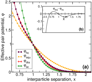
Fig.  1: Isotropic, convex-repulsive potentials, $\varphi_{\text{hc}}$ and $\varphi_{\text{squ}}$ (described in the text), which maximize the density range of mechanically stable 2D honeycomb- and square-lattice ground states, respectively. Also shown are previously designed potentials, $\varphi_{\text{dia}}$ and $\varphi_{\text{sc}}$,Jain et al. (2013a) that maximize the density range of mechanically stable 3D diamond- and simple cubic-lattice ground states, respectively. The inset highlights subtle differences between $\varphi_{\text{dia}}$ and $\varphi_{\text{hc}}$.

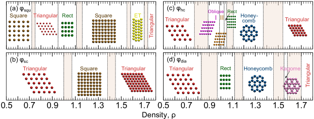
Fig.  2: 2D ground-state lattices as a function of density for (a) $\varphi_{\text{squ}}$, (b) $\varphi_{\text{sc}}$, (c) $\varphi_{\text{hc}}$, and (d) $\varphi_{\text{dia}}$. Shaded regions represent coexistence between the neighboring lattices on the phase diagram. ET represents the elongated triangle Archimedean tiling. Parameters for the oblique and rectangular (Rect) lattices are provided in Table S2 in Supplementary Information.

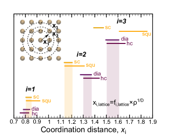
Fig.  3: Separations corresponding to first ($i=1$), second ($i=2$), and third ($i=3$) coordination shells corresponding for stable densities of honeycomb (hc) $\rho=[1.11,1.37]$ and diamond (dia) $\rho=[1.09,1.38]$ ground states for $\varphi_{\text{hc}}$, as well as square (squ) $\rho=[1.16,1.55]$ and simple cubic (sc) $\rho=[1.61,1.95]$ ground states for $\varphi_{\text{squ}}$. The coordination distance ($x_{i}$) for shell $i$ is related to density ($\rho$) by $x_{\text{i,lattice}}=f_{\text{i,lattice}}\times\rho^{\text{1/D}}$, where $D=2$ for hc and squ, and $D=3$ for dia and sc. For hc, $f_{1}=0.877383,f_{2}=\sqrt{3}f_{1},f_{3}=2f_{1}$; for squ, $f_{1}=1,f_{2}=\sqrt{2}f_{1},f_{3}=2f_{1}$; for dia, $f_{1}=0.866025,f_{2}=\sqrt{8/3}f_{1},f_{3}=\sqrt{11/3}f_{1}$; for sc, $f_{1}=1,f_{2}=\sqrt{2}f_{1},f_{3}=\sqrt{3}f_{1}$. Shaded regions indicate overlap of coordination shell distances for analogous 2D and 3D stable lattice ground states.

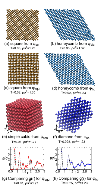
Fig.  4: Snapshots of 2D configurations obtained from Monte Carlo quenches of (a) $\varphi_{\text{sc}}$, (b) $\varphi_{\text{dia}}$, (c) $\varphi_{\text{squ}}$, (d) $\varphi_{\text{hc}}$, and 3D configurations obtained from quenches of (e) $\varphi_{\text{squ}}$, and (f) $\varphi_{\text{hc}}$. For the 3D structures, we plot the corresponding pair distribution functions g(r) of the quenched configurations (dots) and the perfectly equilibrated lattice structures (dashed lines) in (g) and (h), at the specific temperature (T) and density ($\rho$), to demonstrate the structural similarities. The similarity between the annealed and perfectly equilibrated diamond lattice in (h) shows that the annealed structure is not quite defect-free but the configuration energy is only 0.09% higher than that of the perfect lattice. See Table S1 in Supplementary Information.

Supplemental Material: Dimensionality and design of isotropic interactions that stabilize honeycomb, square, simple cubic, and diamond lattices

Table S1: Parameters of the isochoric quenching Monte Carlo simulations.
Notation (symbols) are as presented in the text. Errors in energy magnitudes are $<O(-4)$.

$\varphi_{\text{target}}$	Target-structure	Simulation box	N	$\rho$	$T_{\text{liq}}$	$T_{\text{xtal}}$	$E_{\text{conf}}$	$E_{\text{perf}}$	$\Delta E/E_{\text{perf}}\%$
$\varphi_{\text{hc}}$	honeycomb	20 $\times$ 20	800	1.23	0.1	0.02	3.149555	3.147587	0.062
$\varphi_{\text{dia}}$	honeycomb	20 $\times$ 20	800	1.32	0.1	0.03	3.475706	3.473016	0.077
$\varphi_{\text{squ}}$	square	20 $\times$ 20	400	1.35	0.1	0.02	4.046236	4.045320	0.023
$\varphi_{\text{sc}}$	square	20 $\times$ 20	400	1.23	0.1	0.03	3.396865	3.396758	0.003
$\varphi_{\text{hc}}$	diamond	8 $\times$ 8 $\times$ 8	1024	1.23	0.1	0.025	5.119002	5.114325	0.091
$\varphi_{\text{squ}}$	simple cubic	8 $\times$ 8 $\times$ 8	512	1.77	0.1	0.01	10.225177	10.22514	0.004

Isochoric quenching by Monte Carlo simulations: We first completed a series of canonical Monte Carlo (MC) simulations to estimate the freezing behavior of each model by allowing a perfect lattice interacting with $\varphi_{\text{target}}$, consisting of N particles at density $\rho$, to relax at several temperatures separated by $\Delta T=0.005$. We found that–for all interaction models–at $T_{\text{liq}}=0.1$, the equilibrium structure was the fluid state. We instantaneously quenched these equilibrated disordered configurations to a much lower temperature value $T_{\text{xtal}}$, and allowed the system to evolve for $10^{5}$ MC steps. While some configurations instantaneously assembled to the expected crystal structure, there were also cases where configurations assembled into multiple high-energy defective structures before relaxing toward the final equilibrium structure. The pair distribution functions were averaged over approximately 4000 MC steps after assembly to the final equilibrium structure was achieved. We also simulated the expected crystal (per the ground-state phase diagram) at the same temperature $T_{\text{xtal}}$ and density $\rho$ to provide a comparison of the configurational energy of the quenched configuration $E_{\text{conf}}$ versus the energy of the perfectly equilibrated target lattice $E_{\text{perf}}$. We performed simulations with larger number of particles (upto 4050 particles for honeycomb crystal, 2025 for square crystal, 2500 for diamond crystal and 1300 for simple cubic crystal) for all lattices and also used cuboid box shapes, and found no significant differences in the crystallization behavior and free energies. For $\varphi_{\text{dia}}$, the fluid did not assemble into a perfect diamond crystal within the simulation time. We allowed the system to evolve for $7\times 10^{5}$ MC steps, and no change was seen in the lowest-energy configuration during the final cycle of $10^{5}$ MC steps. However, as can be seen in the table, the energy difference between the perfect diamond crystal and the crystal formed on quenching is about 0.09$\%$, and from Fig. 4 in main text, there are only very subtle discrepancies between the pair distribution function of the quenched configuration and the perfect diamond lattice.

Table S2: 2D ground states for optimized potentials $\varphi_{\text{hc}}$, $\varphi_{\text{squ}}$, $\varphi_{\text{dia}}$ and $\varphi_{\text{sc}}$. Roman numerals denote different structures of the same lattice type.

Lattice	Stability range	Lattice parameters
Honeycomb forming potential, $\varphi_{\text{hc}}$
Triangular	$[0.44,0.77]$
Oblique-I	$[0.89:0.99]$	$b/a:[1.487:1.55]$
		$\theta:[1.227:1.24]$
Oblique-II	$[1.0:1.03]$	$b/a:1.71,\,\theta:1.05$
Rectangular	$[1.03:1.05]$	$b/a:1.49$
Honeycomb	$[1.11:1.37]$
Triangular	$[1.54:2.05]$
Square forming potential, $\varphi_{\text{squ}}$
Square	$[0.5:0.72]$
Triangular	$[0.75:0.95]$
Rectangular	$[0.95:1.11]$	$b/a:[1.43:1.45]$
Square	$[1.16:1.55]$
Elongated Triangular	$[1.58:1.70]$
Triangular	$[1.73:2.15]$
Diamond forming potential, $\varphi_{\text{dia}}$
Triangular	$[0.46:0.83]$
Rectangular	$[0.97:1.12]$	$b/a:\,[1.446:1.526]$
Honeycomb	$[1.19:1.46]$
Kagome	$[1.55:1.58]$
Triangular	$[1.70:2.09]$
Simple cubic forming potential, $\varphi_{\text{sc}}$
Triangular	$[0.5:1.0]$
Square	$[1.07:1.38]$
Triangular	$[1.45:1.8]$

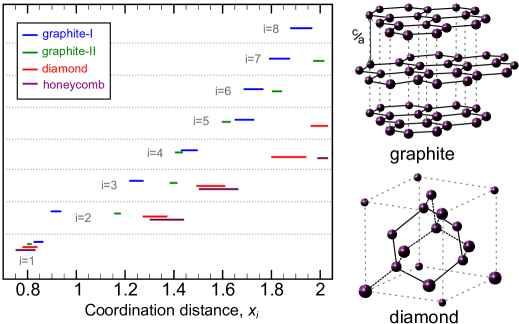
Fig.  S1: Interparticle separations corresponding to the $i^{th}$ coordination shells ($i$=1, 2, 3…) of honeycomb, diamond, graphite-I, and graphite-II lattices within the interaction range for the potential $\varphi_{\text{hc}}$. Coordination-shell distances for honeycomb $\rho=[1.11,1.37]$ and diamond $\rho=[1.09,1.38]$ correspond to their stability ranges for $\varphi_{\text{hc}}$ (see Fig. 3). For graphite-I (c/a=1.27) $\rho=[1.1,1.26]$ and graphite-II (c/a=1.67) $\rho=[0.98,1.05]$ lattices, the distances correspond to the density range at which each lattice is mechanically stable (i.e. the lowest phonon frequency has a positive value). We also highlight the honeycomb motif in the graphite and the diamond structures.

In Fig. S1, we plot the interparticle separations corresponding to the coordination shells of honeycomb, diamond and graphite structures within the interaction range for $\varphi_{\text{hc}}$. Graphite structures with axial ratios (c/a) in the ranges $[1.64,1.69]$ and $[1.25,1.27]$ are found to be optimal and mechanically stable in the density range of interest. However, on comparison with a larger pool of structures, A7-II and diamond (see Table I) have lower molar enthalpy and are chemically stable. We clearly see that there is no coordination-shell overlap beyond the nearest neighbour distances for all the four lattices, and hence, $\varphi_{\text{hc}}$ is not able to stabilize any of the graphite structures.

References

- Zhang et al. (2010) Junhu Zhang, Yunfeng Li, Xuemin Zhang, and Bai Yang, “Colloidal self-assembly meets nanofabrication: From two-dimensional colloidal crystals to nanostructure arrays,” Adv. Mat. 22, 4249–4269 (2010).
- Wu et al. (2012) Dingcai Wu, Fei Xu, Bin Sun, Ruowen Fu, Hongkun He, and Krzysztof Matyjaszewski, “Design and preparation of porous polymers,” Chem. Rev. 112, 3959–4015 (2012).
- Wang et al. (2006) C C Wang, A O Adeyeye, and N Singh, “Magnetic antidot nanostructures: effect of lattice geometry,” Nanotechnology 17, 1629 (2006).
- Xia et al. (2000) Y. Xia, B. Gates, Y. Yin, and Y. Lu, “Monodispersed colloidal spheres: Old materials with new applications,” Adv. Mat. 12, 693–713 (2000).
- Furumi et al. (2010) Seuchi Furumi, Hiroshi Fudouzi, and Tsutomu Sawada, “Self-organized colloidal crystals for photonics and laser applications,” Laser & Photon. Rev. 4, 205–220 (2010).
- von Freymann et al. (2013) Georg von Freymann, Vladimir Kitaev, Bettina V. Lotschz, and Geoffrey A. Ozin, “Bottom-up assembly of photonic crystals,” Chem. Soc. Rev. 42, 2528–2554 (2013).
- Murray et al. (2000) Christopher B Murray, CR Kagan, and MG Bawendi, “Synthesis and characterization of monodisperse nanocrystals and close-packed nanocrystal assemblies,” Annu. Rev. Mater. Sci. 30, 545–610 (2000).
- Kim et al. (2013) Jin Young Kim, Oleksandr Voznyy, David Zhitomirsky, and Edward H. Sargent, “25th anniversary article: Colloidal quantum dot materials and devices: A quarter-century of advances,” Adv. Mat. 25, 4986–5010 (2013).
- Glotzer and Solomon (2007) S.C. Glotzer and M.J. Solomon, “Anisotropy of building blocks and their assembly into complex structures,” Nat. Mater. 6, 557–562 (2007).
- Xia et al. (2009) Younan Xia, Yujie Xiong, Byungkwon Lim, and Sara E. Skrabalak, “Shape-controlled synthesis of metal nanocrystals: Simple chemistry meets complex physics?” Angew. Chem. Int. Edit. 48, 60–103 (2009).
- Damasceno et al. (2012) Pablo F. Damasceno, Michael Engel, and Sharon C. Glotzer, “Predictive self-assembly of polyhedra into complex structures,” Science 337, 453–457 (2012).
- Agarwal and Escobedo (2011) Umang Agarwal and Fernando A. Escobedo, “Mesophase behaviour of polyhedral particles,” Nat. Mater. 10, 230–235 (2011).
- Henzie et al. (2012) Joel Henzie, Michael Gruenwald, Asaph Widmer-Cooper, Phillip L. Geissler, and Peidong Yang, “Self-assembly of uniform polyhedral silver nanocrystals into densest packings and exotic superlattices,” Nat. Mater. 11, 131–137 (2012).
- Quan et al. (2014) Zewei Quan, Hongwu Xu, Chenyu Wang, Xiaodong Wen, Yuxuan Wang, Jinlong Zhu, Ruipeng Li, Chris J. Sheehan, Zhongwu Wang, Detlef-M. Smilgies, Zhiping Luo, and Jiye Fang, “Solvent-mediated self-assembly of nanocube superlattices,” J. Am. Chem. Soc. 136, 1352–1359 (2014).
- Sacanna et al. (2013) Stefano Sacanna, David J. Pine, and Gi-Ra Yi, “Engineering shape: the novel geometries of colloidal self-assembly,” Soft Matter 9, 8096–8106 (2013).
- Vega and Monson (1998) C. Vega and P. A. Monson, “Solid–fluid equilibrium for a molecular model with short ranged directional forces,” J. Chem. Phys. 109, 9938–9949 (1998).
- Kraft et al. (2012) Daniela J. Kraft, Ran Ni, Frank Smallenburg, Michiel Hermes, Kisun Yoon, David A. Weitz, Alfons van Blaaderen, Jan Groenewold, Marjolein Dijkstra, and Willem K. Kegel, “Surface roughness directed self-assembly of patchy particles into colloidal micelles,” Proc. Nat. Acad. Sci. USA 109, 10787–10792 (2012).
- Yi et al. (2013) Gi-Ra Yi, David J. Pine, and Stefano Sacanna, “Recent progress on patchy colloids and their self-assembly,” J. Phys.:Condens. Matter 25 (2013).
- Jayaraman (2013) Arthi Jayaraman, “Polymer grafted nanoparticles: Effect of chemical and physical heterogeneity in polymer grafts on particle assembly and dispersion,” J. Polym. Sci. Part B: Polym. Phys. 51, 524–534 (2013).
- Courty et al. (2011) Alexa Courty, Johannes Richardi, Pierre-Antoine Albouy, and Marie-Paule Pileni, “How to control the crystalline structure of supracrystals of 5-nm silver nanocrystals,” Chem. Mater. 23, 4186–4192 (2011).
- Shevchenko et al. (2006) Elena V Shevchenko, Dmitri V Talapin, Nicholas A Kotov, Stephen O’Brien, and Christopher B Murray, “Structural diversity in binary nanoparticle superlattices,” Nature (London) 439, 55–59 (2006).
- Pavan et al. (2012) Mariela J. Pavan, Elina Ploshnik, and Roy Shenhar, “Nanoparticle assembly on topographical polymer templates: Effects of spin rate, nanoparticle size, ligand, and concentration,” J. Phys. Chem. B 116, 13922–13931 (2012).
- Kinge et al. (2008) Sachin Kinge, Mercedes Crego-Calama, and David N. Reinhoudt, “Self-assembling nanoparticles at surfaces and interfaces,” Chem. Phys. Chem. 9, 20–42 (2008).
- Ho et al. (1990) K. M. Ho, C. T. Chan, and C. M. Soukoulis, “Existence of a photonic gap in periodic dielectric structures,” Phys. Rev. Lett. 65, 3152–3155 (1990).
- Sözüer and Haus (1993) H. Sami Sözüer and Joseph W. Haus, “Photonic bands: Simple-cubic lattice,” J. Opt. Soc. Am. B 10, 296–302 (1993).
- Yoshida and Kamakura (1972) Takeshi Yoshida and Shiro Kamakura, “Theory of melting at high pressures. II,” Prog. Theor. Phys. 47, 1801–1816 (1972).
- Fomin et al. (2008) Yu. D. Fomin, N. V. Gribova, V. N. Ryzhov, S. M. Stishov, and Daan Frenkel, “Quasibinary amorphous phase in a three-dimensional system of particles with repulsive-shoulder interactions,” J. Chem. Phys. 129, 064512 (2008).
- Marcotte et al. (2013) É. Marcotte, F. H. Stillinger, and Salvatore Torquato, “Communication: Designed diamond ground state via optimized isotropic monotonic pair potentials,” J. Chem. Phys. 138, 061101 (2013).
- Edlund et al. (2013) E. Edlund, O. Lindgren, and M. Nilsson Jacobi, “Using the uncertainty principle to design simple interactions for targeted self-assembly,” J. Chem. Phys. 139, 024107 (2013).
- Jain et al. (2013a) Avni Jain, Jeffrey R. Errington, and Thomas M. Truskett, “Inverse design of simple pairwise interactions with low-coordinated 3D lattice ground states,” Soft Matter 9, 3866–3870 (2013a).
- Pàmies et al. (2009) Josep C. Pàmies, Angelo Cacciuto, and Daan Frenkel, “Phase diagram of hertzian spheres,” J. Chem. Phys. 131, 044514 (2009).
- Watzlawek et al. (1999) M. Watzlawek, C. N. Likos, and H. Löwen, “Phase diagram of star polymer solutions,” Phys. Rev. Lett. 82, 5289–5292 (1999).
- Jagla (1999) E. A. Jagla, “Minimum energy configurations of repelling particles in two dimensions,” J. Chem. Phys. 110 (1999).
- Camp (2003) Philip J. Camp, “Structure and phase behavior of a two-dimensional system with core-softened and long-range repulsive interactions,” Phys. Rev. E 68, 061506 (2003).
- Malescio and Pellicane (2003) G Malescio and G Pellicane, “Stripe phases from isotropic repulsive interactions,” Nat. Mater. 2, 97–100 (2003).
- Marcotte et al. (2011a) É. Marcotte, F. H. Stillinger, and S. Torquato, “Unusual ground states via monotonic convex pair potentials,” J. Chem. Phys. 134, 164105 (2011a).
- Zhang et al. (2013) G. Zhang, F. H. Stillinger, and S. Torquato, “Probing the limitations of isotropic pair potentials to produce ground-state structural extremes via inverse statistical mechanics,” Phys. Rev. E 88, 042309 (2013).
- Lafitte et al. (2014) Thomas Lafitte, Sanat K. Kumar, and Athanassios Z. Panagiotopoulos, “Self-assembly of polymer-grafted nanoparticles in thin films,” Soft Matter 10, 786–794 (2014).
- Dudalov et al. (2014) D.E. Dudalov, Yu.D. Fomin, E.N. Tsiok, and V.N. Ryzhov, “Anomalous melting scenario of the two-dimensional core-softened system,” Phys. Rev. Lett. 112, 157803 (2014).
- Osterman et al. (2007) N. Osterman, D. Babič, I. Poberaj, J. Dobnikar, and P. Ziherl, “Observation of condensed phases of quasiplanar core-softened colloids,” Phys. Rev. Lett. 99, 248301 (2007).
- Chen et al. (2011) Qian Chen, Sung Chul Bae, and Steve Granick, “Directed self-assembly of a colloidal kagome lattice,” Nature (London) 469, 381–384 (2011).
- Evers et al. (2013) Wiel H. Evers, Bart Goris, Sara Bals, Marianna Casavola, Joost de Graaf, René van Roij, Marjolein Dijkstra, and Daniël Vanmaekelbergh, “Low-dimensional semiconductor superlattices formed by geometric control over nanocrystal attachment,” Nano Lett. 13, 2317–2323 (2013).
- Antlanger et al. (2011) Moritz Antlanger, Günther Doppelbauer, and Gerhard Kahl, “On the stability of Archimedean tilings formed by patchy particles,” J. Phys.: Condens. Matter 23, 404206 (2011).
- Millan et al. (2014) Jaime A. Millan, Daniel Ortiz, Greg van Anders, and Sharon C. Glotzer, “Self-assembly of Archimedean tilings with enthalpically and entropically patchy polygons,” ACS Nano 8, 2918–2928 (2014).
- Bianchi et al. (2011) Emanuela Bianchi, Ronald Blaak, and Christos N. Likos, “Patchy colloids: state of the art and perspectives,” Phys. Chem. Chem. Phys. 13, 6397–6410 (2011).
- Romano and Sciortino (2012) Flavio Romano and Francesco Sciortino, “Patterning symmetry in the rational design of colloidal crystals,” Nat. Commun. 3, 975 (2012).
- Note (1) The term ‘analogous structures’ refers to the pairs of 2D-3D lattices (e.g., honeycomb-diamond and square-simple cubic) that have specific coordination-shell similarities that can allow a single isotropic pair potential to favor the stability of both. This structural similarity is addressed both in the discussion of Fig. 3 and Fig. S1 (in the Supplementary Information).
- Torquato (2009) Salvatore Torquato, “Inverse optimization techniques for targeted self-assembly,” Soft Matter 5, 1157–1173 (2009).
- (49) Avni Jain, Jonathan A. Bollinger, and Thomas M. Truskett, “Perspective: Inverse methods for material design,” AIChE J. 10.1002/aic.14491.
- Note (2) We note that particles confined to a 2D monolayer, such as at a liquid-liquid interface or on a substrate, may interact via an effective pair potential that is different from the one that the same particles experience in a 3D bulk fluid.
- Schapotschnikow et al. (2008) Philipp Schapotschnikow, René Pool, and Thijs JH Vlugt, “Molecular simulations of interacting nanocrystals,” Nano Lett. 8, 2930–2934 (2008).
- Gottwald et al. (2005) Dieter Gottwald, Gerhard Kahl, and Christos N. Likos, “Predicting equilibrium structures in freezing processes.” J. Chem. Phys. 122, 204503 (2005).
- Bianchi et al. (2012) Emanuela Bianchi, Günther Doppelbauer, Laura Filion, Marjolein Dijkstra, and Gerhard Kahl, “Predicting patchy particle crystals: Variable box shape simulations and evolutionary algorithms,” J. Chem. Phys. 136, 214102 (2012).
- Phillips and Voth (2013) Carolyn L. Phillips and Gregory A. Voth, “Discovering crystals using shape matching and machine learning,” Soft Matter 9, 8552–8568 (2013).
- Ashcroft and Mermin (1976) N.W. Ashcroft and N.D. Mermin, Solid State Physics (Saunders College, Philadelphia, 1976).
- Prestipino et al. (2009) Santi Prestipino, Franz Saija, and Gianpietro Malescio, “The zero-temperature phase diagram of soft-repulsive particle fluids,” Soft Matter 5, 2795–2803 (2009).
- Note (3) Using the approach outlined in the text, the competitive pools determined for use in optimizations targeting the honeycomb lattice consisted of triangular, square, kagome, snub-square, elongated triangular, rectangular (), rectangular (), rectangular (), rectangular (), and snub-hexagonal lattices. For the square lattice, the final pool comprised triangular, oblique (, =1.234), kagome, honeycomb, elongated triangular, snub-hexagonal, and snub-square lattices. For diamond, the pool Jain et al. (2013a) consisted of FCC, WUR, SH , Sn , Sn , A7 , and A20 lattices. For simple cubic, the pool Jain et al. (2013a) comprised FCC, BCC, DIA, SH , SH , SH , A20 , Sn , Sn , and Sn lattices. Here, and denote the aspect ratio of the sides of the unit cell, and is the angle between the two sides. The other symbols and , we adopt here, are the same as those used in a previous study Prestipino et al. (2009).
- Jain et al. (2013b) Avni Jain, Jeffrey R. Errington, and Thomas M. Truskett, “Communication: Phase behavior of materials with isotropic interactions designed by inverse strategies to favor diamond and simple cubic lattice ground states,” J. Chem. Phys. 139, 141102 (2013b).
- Note (4) Optimal parameters for the honeycomb-forming interaction are , , , , , , , , , , , and . For the square-forming potential , they are , , , , , , , , , , , and .
- Note (5) Also see Table S2 in Supplemental Information which tabulates the stable ground-state lattices with their corresponding density ranges and lattice parameters.
- Marcotte et al. (2011b) E. Marcotte, F. H. Stillinger, and S. Torquato, “Optimized monotonic convex pair potentials stabilize low-coordinated crystals,” Soft Matter 7, 2332–2335 (2011b).
- Note (6) Ground states and finite-temperature phase boundaries for and have been determined previously and are presented in detail elsewhere Jain et al. (2013a, b).
- van Meel et al. (2009a) J. A. van Meel, D. Frenkel, and P. Charbonneau, “Geometrical frustration: A study of four-dimensional hard spheres,” Phys. Rev. E 79, 030201 (2009a).
- van Meel et al. (2009b) J. A. van Meel, B. Charbonneau, A. Fortini, and P. Charbonneau, “Hard-sphere crystallization gets rarer with increasing dimension,” Phys. Rev. E 80, 061110 (2009b).