Polyakov loop spectroscopy in the confined phase of gluodynamics and QCD

Abstract

By using a simple relativistic model, we compute the glueball and gluelump spectra and relate these quantities, respectively, to the trace anomaly and Polyakov loop in the adjoint representation of gluodynamics. This spectroscopic description of thermodynamics is extended with the inclusion of quarks. The relation between the hadron resonance gas and the Polyakov loop in the fundamental and higher representations is addressed.

1 Introduction

The confined phase of SU($N_{c}$) non-Abelian gauge theories can be naturally described in terms of their relevant degrees of freedom in this regime. In gluodynamics and QCD these are bound states of gluons and quarks, i.e. glueballs and hadrons. By neglecting the interaction between these states in the plasma, the hadron resonance gas model appears as a natural picture that can describe the thermodynamics of these theories with a surprising accuracy [1, 2, 3, 4, 5, 6, 7].

The trace anomaly signals the breaking of scale invariance, and it is a key quantity to study the thermodynamics of QCD [8]. Other quantity of interest is the Polyakov loop (PL) in the fundamental representation, commonly used as an order parameter for the confinement/deconfinement of color charges [9]. While the interplay between the PL and physical observables has been considered obscure for a long time, recent advances have led to a description of the PL in terms of hadronic resonances, making a clear connection between this quantity and the spectrum of QCD [10, 11, 12]. In this communication we will elaborate on this relation in gluodynamics and QCD, and provide a physical interpretation of the PL in representations other than the fundamental one.

2 Glueballs, gluelumps and thermodynamics

Gluodynamics (and QCD) predicts the self-coupling of gluons. The natural consequence is the possible existence of bound states with no quarks, the so-called glueballs [13]. Paralleling lattice studies (see e.g. [14]), some models have been proposed to describe the lowest-lying states [15, 16, 17]. We will study a simple relativistic model to obtain an overall description of the glueball spectrum of two gluons. The model can be easily extended to study the gluelumps: multigluonic states with one static gluon. We will use the spectrum to compute the thermodynamics.

2.1 Glueball Spectrum and Trace Anomaly

The glueball is a bound state of two or more dynamical gluons. We consider a relativistic model of two massless gluons. The Hamiltonian writes

$$H_{[gg]}=|\vec{p_{1}}|+|\vec{p_{2}}|+V(r_{12})\,,$$ (1)

where the potential $V$ depends only on the relative distance between the gluons. The classical partition function writes

$$\log Z^{\textrm{\scriptsize cl}}_{[gg]}=\frac{\gamma^{2}}{2}\int\frac{d^{3}x_{1}d^{3}p_{1}}{(2\pi)^{3}}\frac{d^{3}x_{2}d^{3}p_{2}}{(2\pi)^{3}}e^{-H_{[gg]}/T}+\cdots,$$ (2)

where $\gamma$ is the gluon spin degeneracy and the dots stand for 3 and higher gluon terms which will be neglected. In what follows we assume a gluon-gluon potential of the form $V(r)=\sigma_{8}r$, with Casimir scaling between the adjoint and fundamental representation string tensions $\sigma_{8}=\frac{N_{c}^{2}}{4}\sigma_{3}$. The trace anomaly is obtained from the standard thermodynamic relation

$$\Delta(T)\equiv T\frac{\partial}{\partial T}\left(\frac{P}{T^{4}}\right)=\frac{\varepsilon-3P}{T^{4}}\,,\quad Z=e^{PV/T}.$$ (3)

After an explicit evaluation of Eq. (2), the classical result for the trace anomaly in gluodynamics is

$$\Delta^{\textrm{\scriptsize cl}}_{[gg]}(T)=\frac{\gamma^{2}}{2}\frac{48}{\pi^{3}\sigma_{8}^{3}}T^{6}\,.$$ (4)

In order to isolate the relative motion and deal with a simpler quantum Hamiltonian, it is convenient to transform (2) by applying the identity [18]

$$e^{-|\vec{p}|/T}=\frac{1}{\sqrt{\pi T}}\int_{0}^{\infty}\frac{d\mu}{\sqrt{\mu}}e^{-\frac{1}{T}\,\left(\frac{\vec{p}^{2}}{4\mu}+\mu\right)}$$ (5)

to both gluons. Integrating out the center of mass gives

$$\frac{\log Z^{\textrm{\scriptsize cl}}_{[gg]}}{V}\!=\!\frac{4\sqrt{T}}{3\pi^{5/2}}\!\!\int_{0}^{\infty}\!\!\!\!\!d\mu\mu^{3/2}e^{-\frac{\mu}{T}}\frac{\gamma^{2}}{2}\!\!\int\!\!\frac{d^{3}xd^{3}p}{(2\pi)^{3}}e^{-\frac{1}{T}\left(\frac{\vec{p}^{2}}{\mu}+V(r)\right)}$$ (6)

This auxiliary system can now be quantized by applying standard quantization rules. Then, Eq. (6) transforms into the quantum partition function

$$\frac{\log Z_{[gg]}}{V}\!=\!\frac{4\sqrt{T}}{3\pi^{5/2}}\!\!\int_{0}^{\infty}\!\!\!\!d\mu\mu^{3/2}e^{-\frac{\mu}{T}}\!\!\sum_{n,l}\nu_{l}(2l+1)e^{-\frac{1}{T}\frac{\sigma_{8}^{2/3}}{\mu^{1/3}}\varepsilon_{n,l}},$$ (7)

where $\nu_{l}=\gamma(\gamma\pm 1)/2$ for even/odd $l$ and the spectrum is readily obtained from the Schrödinger equation

$$\left(-\nabla^{2}+r\right)\Psi_{n,l}=\varepsilon_{n,l}\Psi_{n,l}\,.$$ (8)

We plot in Fig. 1 the result of the trace anomaly by using Eqs. (7)-(8).

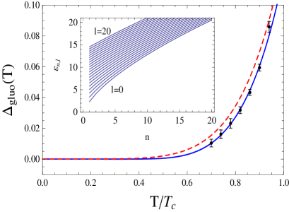
Figure 1: Trace anomaly of gluodynamics as a function of temperature (in units of $T_{c}$). We plot as continuous (blue) line the quantum result from Eqs. (7)-(8), and as dashed (red) line the classical result, Eq. (4). We use $\gamma=3$. Lattice data have been taken from [19]. The inserted figure corresponds to the spectrum obtained with Eq. (8).

We have fitted the lattice data by considering as the sole fitting parameter the dimensionless ratio $T_{c}/\sqrt{\sigma_{3}}$. The result is $T_{c}/\sqrt{\sigma_{3}}=0.774$ and $\chi^{2}/\textrm{dof}=0.54$, in the regime $0.70<T/T_{c}<0.94$ with $\gamma=3$. It is noteworthy that such a simple model leads to a value which is similar to the one reported from lattice computations $T_{c}/\sqrt{\sigma_{3}}\approx 0.629(3)$ [19]. The agreement between classical and quantum results for temperatures $T\gtrsim 0.7T_{c}$ can be improved by including the first semiclassical correction.

2.2 Gluelump spectrum and Polyakov loop

The similar model for the gluelump spectrum (an adjoint source dressed by dynamical gluons) in the leading approximation (just one gluon) has the Hamiltonian

$$H_{[Gg]}=|\vec{p}|+V(r)\,.$$ (9)

Simple scaling shows that $M_{Gg}=M_{g}/\sqrt{2}$ for the ground states of glueball and gluelump in the $\sigma_{8}r$ model. A remarkable consequence is that, strictly speaking, the smallest mass gap in gluodynamics is not the lightest glueball mass but the lightest gluelump mass.

Straightforward integration in the equation similar to (2) gives the explicit result for the classical partition function

$$L_{\bf 8}(T)\approx\log Z^{\textrm{\scriptsize cl}}_{[Gg]}=\gamma\frac{8}{\pi\sigma_{8}^{3}}T^{6}\,,$$ (10)

where $L_{\bf 8}$ is the adjoint PL [12]. From a comparison of Eqs. (4) and (10), one gets the approximate scaling $L_{\bf 8}(T)\approx\frac{\pi^{2}}{3\gamma}\Delta_{[gg]}(T)$.

The quantum version, similar to (7), for the partition function of the gluelump is

$$\log Z_{[Gg]}=\gamma\int_{0}^{\infty}\!\!\!\!\frac{d\mu}{\sqrt{\pi T\mu}}e^{-\frac{\mu}{T}}\!\!\sum_{n,l}(2l+1)e^{-\left(\frac{\sigma_{8}^{2}}{4\mu}\right)^{1/3}\frac{\varepsilon_{n,l}}{T}},$$ (11)

with the same eigenvalues $\varepsilon_{n,l}$ as in Eq. (8).

The ratio between the adjoint PL and the trace anomaly computed with the model is plotted in Fig. 2. The approximate classical scaling $\pi^{2}/3\gamma$ is valid for temperatures $T\gtrsim 0.5T_{c}$.

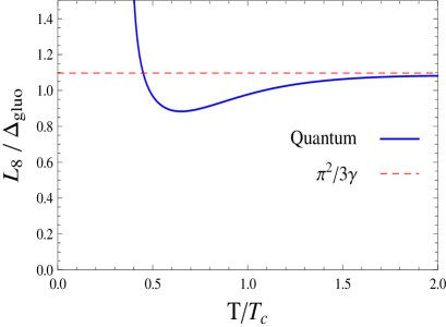
Figure 2: Ratio between PL in the adjoint representation and trace anomaly, as a function of temperature (in units of $T_{c}$). Continuous (blue) line is the quantum result from Eqs. (7)-(8) and (11). Dashed (red) line is the approximate classical scaling $\pi^{2}/3\gamma$. We use $\gamma=3$.

3 QCD thermodynamics and Polyakov loop

An effective approach to QCD at finite temperature is provided by chiral quark models coupled to the Polyakov loop [20, 21, 22, 23, 24, 25]. While the mean field approximation is widely used to study the phase transition, it was stressed in [21, 26, 22, 27, 28] that local and quantum corrections of the PL are needed at low temperatures. We will use this approach to derive the relation between the QCD spectrum and the PL in fundamental and higher representations.

3.1 Polyakov-Constituent Quark Model

The partition function of the model is [21, 29, 30, 31, 12]

$$Z=\int{\cal D}\Omega{\cal D}\bar{q}{\cal D}q\,e^{-S_{g}(T,\Omega)-S_{q}(T,\Omega)}\,,$$ (12)

where the gluonic and quark actions read

$$S_{g}=-2T\!\!\int\!\!\frac{d^{3}xd^{3}p}{(2\pi)^{3}}{\rm tr}\log\left(1\!-\!\Omega_{8}(\vec{x})\,e^{-E_{p}/T}\right)\,,$$ (13)

$$S_{q}=2N_{f}\!\!\int\!\!\frac{d^{3}xd^{3}p}{(2\pi)^{3}}\bigg{(}{\rm tr}\log\big{[}1\!+\!\Omega_{3}(\vec{x})\,e^{-E_{p}/T}\big{]}\!+\!h.c.\bigg{)}\,.$$ (14)

The PL variables $\Omega_{\mu}(\vec{x})$ and $\Omega_{\mu}^{\dagger}(\vec{x})$ play the role of quark and gluon creation/annihilation operators. A series expansion of the action in powers of these operators leads to an expansion in the number of constituents, and each term can be identified with a multi-quark(gluon) state. In particular the meson contribution to the partition function follows from the correlator $Z_{[q\bar{q}]}\!\sim\!\langle{\rm tr}\,\Omega_{3}(x){\rm tr}\,\Omega_{3}^{\dagger}(x^{\prime})\rangle\!\sim\!e^{-(M_{q}+M_{\bar{q}})/T}$. After quantization as in Sec. 2, the Boltzmann factor at low temperature will contain the spectrum of mesons. There are also contributions from baryons, glueballs, etc. If we neglect the interaction between hadrons and retain only the confining forces, one has $Z\simeq Z_{[q\bar{q}]}Z_{[qqq]}Z_{[gg]}\cdots$. This approximation, known as the Hadron Resonance Gas (HRG) model, has been widely used to describe the confined phase of QCD with a remarkable agreement to lattice data [8, 7].

3.2 Hadron Resonance Gas model and Polyakov loop

The partition function described above corresponds to a plasma formed by dynamical constituents. An alternative physical system appears when one considers in the plasma a static color source (heavy quark) in position $x_{0}$ and representation ${\bf 3}$. This source polarizes the medium, as it becomes screened by dynamical quarks and gluons to form a heavy-light hadron which is color neutral. The consequence is that the partition function of this system receives contributions of the form

$$Z_{[Q\bar{q}]}\!\sim\!\langle{\rm tr}\,\Omega_{3}(x_{0})\,{\rm tr}\,\Omega_{3}^{\dagger}(x^{\prime})\rangle\!\sim\!e^{-(M_{Q}+M_{\bar{q}})/T}\,,$$ (15)

$$Z_{[Qqq]}\!\!\sim\!\!\langle{\rm tr}\,\Omega_{3}(x_{0})\,{\rm tr}\,\Omega(x^{\prime})\,{\rm tr}\,\Omega(x^{\prime\prime})\rangle\!\sim\!e^{-(M_{Q}+2M_{q})/T}\,,$$ (16)

$$Z_{[Q\bar{q}g]}\!\!\sim\!\langle{\rm tr}\Omega_{3}(x_{0})\,{\rm tr}\Omega_{3}^{\dagger}(x^{\prime})\,{\rm tr}\Omega_{8}(x^{\prime\prime})\rangle\!\sim\!\!e^{-(M_{Q}+M_{\bar{q}}+M_{g})/T}$$ (17)

After quantization and renormalization [32], one gets the HRG model for the PL in the representation ${\bf 3}$, which can be written as

$$L_{\bf 3}\simeq Z_{[Q\bar{q}]}Z_{[Qqq]}Z_{[Q\bar{q}g]}\cdots\simeq\frac{1}{2N_{c}}\sum_{[Q\alpha]}g_{[Q\alpha]}e^{-\Delta_{[Q\alpha]}/T}\,,$$ (18)

where $\Delta_{[Q\alpha]}=\lim_{m_{Q}\to\infty}(M_{[Q\alpha]}-m_{Q})$. In these formulas $[Q\alpha]$ stands for the spectrum of heavy-light hadrons, and $m_{Q}$ is the mass of the heavy quark. The fact that the PL corresponds to a partition function explains its real and positive character. This approach was first proposed in [10], and it describes very well the lattice data for the PL in the fundamental representation in the confined phase when a large enough amount of states are included in the spectrum [10, 11].

It is possible to generalize this model to the PL in any representation $\mu$. In this case $Q$ is replaced by a static source in the representation $\mu$, which we denote by $S_{\mu}$, and it is screened by dynamical constituents to form color neutral states according to a specific pattern which depends on $\mu$ [12]. The result is

$$L_{\mu}\simeq\frac{1}{2N_{c}}\sum_{[S_{\mu}\alpha]}g_{[S_{\mu}\alpha]}e^{-\Delta_{[S_{\mu}\alpha]}/T}\,.$$ (19)

We show in Fig. 3 the PL in several representations computed with the Polyakov-Constituent Quark model.

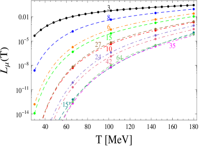
Figure 3: Polyakov loop in several representations as a function of $T$ (in $\,{\rm MeV}$). From top to bottom $\mu={\bf 3}$, ${\bf 8}$, ${\bf 6}$, ${\bf 15}$, ${\bf 27}$, ${\bf 10}$, ${\bf 24}$, ${\bf 42}$, ${\bf 64}$, ${\bf 15^{\prime}}$, and ${\bf 35}$. We consider $N_{f}=2$, $M_{q}=300\,\,{\rm MeV}$ and $M_{g}=664\,\,{\rm MeV}$.

The low temperature behavior is dominated by the lightest energy gap associated with the screening of heavy sources, and as such, implements particular scaling rules between the PL in different representations, which in general are different from the Casimir scaling [33]. A list of alternative low temperature scaling rules has been identified in [12], and could be tested by lattice calculations.

4 Discussion and outlook

The previous considerations provide interesting guidelines to model not only the trace anomaly but also the interesting physical situation appearing when a static color source is placed in the hot but confined medium. In this case the medium becomes polarized in the color degrees of freedom, as dynamical colored particles tend to screen the source. The partition function of this system is related to the expectation value of the PL in the group representation of the static source and admits a hadronic representation in terms of bound states in which the source appears as one of the constituents. The natural extension to QCD allows the static source to be either a quark, gluon or combination of both, and the spectrum is formed by conventional heavy-light hadrons, and possibly hybrid and exotic states. From this point of view, the possibility of using the Polyakov loop in higher representations than the fundamental one, emerges as a fascinating opportunity to study the spectroscopy of QCD, including excited states, exotics and hybrids which could be tested on the lattice.

References

- [1] R. Hagedorn, Lect. Notes Phys. 221 (1985) 53–76.
- [2] V. Yukalov, E. Yukalova, Phys. Part. Nucl. 28 (1997) 37–65.
- [3] N. O. Agasian, Phys. Lett. B519 (2001) 71–77.
- [4] A. Tawfik, Phys. Rev. D71 (2005) 054502.
- [5] S. Borsanyi, G. Endrodi, Z. Fodor, A. Jakovac, S. D. Katz, et al., JHEP 1011 (2010) 077.
- [6] A. Bazavov, et al., Phys. Rev. D85 (2012) 054503.
- [7] E. Megias, E. Ruiz Arriola, L.L. Salcedo, Nucl. Phys. Proc. Suppl. 234 (2013) 313–316.
- [8] A. Bazavov, T. Bhattacharya, M. Cheng, N. Christ, C. DeTar, et al., Phys. Rev. D80 (2009) 014504.
- [9] B. Svetitsky, Phys. Rept. 132 (1986) 1–53.
- [10] E. Megias, E. Ruiz Arriola, L.L. Salcedo, Phys. Rev. Lett. 109 (2012) 151601.
- [11] A. Bazavov, P. Petreczky, Phys. Rev. D87 (9) (2013) 094505.
- [12] E. Megias, E. Ruiz Arriola, L.L. Salcedo, Phys. Rev. D89 (2014) 076006.
- [13] W. Ochs, J. Phys. G40 (2013) 043001.
- [14] B. Lucini, PoS QCD-TNT-III (2013) 023.
- [15] F. Brau, C. Semay, Phys. Rev. D70 (2004) 014017.
- [16] V. Mathieu, C. Semay, B. Silvestre-Brac, Phys. Rev. D77 (2008) 094009.
- [17] F. Buisseret, V. Mathieu, C. Semay, Phys. Rev. D80 (2009) 074021.
- [18] D. Antonov, S. Domdey, H.-J. Pirner, Nucl. Phys. Proc. Suppl. 174 (2007) 221–224.
- [19] S. Borsanyi, G. Endrodi, Z. Fodor, S. Katz, K. Szabo, JHEP 1207 (2012) 056.
- [20] K. Fukushima, Phys. Lett. B591 (2004) 277–284.
- [21] E. Megias, E. Ruiz Arriola, L.L. Salcedo, Phys. Rev. D74 (2006) 065005.
- [22] E. Megias, E. Ruiz Arriola, L.L. Salcedo, Phys. Rev. D74 (2006) 114014.
- [23] C. Ratti, M. A. Thaler, W. Weise, Phys. Rev. D73 (2006) 014019.
- [24] M. Dutra, O. Lourenço, A. Delfino, T. Frederico, M. Malheiro, Phys. Rev. D88 (11) (2013) 114013.
- [25] M. Ferreira, P. Costa, D. P. Menezes, C. Providência, N. Scoccola, Phys. Rev. D89 (2014) 016002.
- [26] E. Megias, E. Ruiz Arriola, L.L. Salcedo, PoS JHW2005 (2006) 025.
- [27] E. Megias, E. Ruiz Arriola, L.L. Salcedo, AIP Conf. Proc. 892 (2007) 444–447.
- [28] E. Megias, E. Ruiz Arriola, L.L. Salcedo, Eur. Phys. J. A31 (2007) 553–556.
- [29] C. Sasaki, K. Redlich, Phys. Rev. D86 (2012) 014007.
- [30] E. Megias, E. R. Arriola, L.L. Salcedo, EPJ Web Conf. 66 (2014) 04021.
- [31] E. Megias, E. R. Arriola, L.L. Salcedo, (2013), 1310.3079.
- [32] E. Ruiz Arriola, E. Megias, L.L. Salcedo, AIP Conf. Proc. 1520 (2013) 185–190.
- [33] S. Gupta, K. Huebner, O. Kaczmarek, Phys. Rev. D77 (2008) 034503.