Escaping Local Optima in a Class of Multi-Agent Distributed Optimization Problems: A Boosting Function Approach

Abstract

We address the problem of multiple local optima commonly arising in optimization problems for multi-agent systems, where objective functions are nonlinear and nonconvex. For the class of coverage control problems, we propose a systematic approach for escaping a local optimum, rather than randomly perturbing controllable variables away from it. We show that the objective function for these problems can be decomposed to facilitate the evaluation of the local partial derivative of each node in the system and to provide insights into its structure. This structure is exploited by defining “boosting functions” applied to the aforementioned local partial derivative at an equilibrium point where its value is zero so as to transform it in a way that induces nodes to explore poorly covered areas of the mission space until a new equilibrium point is reached. The proposed boosting process ensures that, at its conclusion, the objective function is no worse than its pre-boosting value. However, the global optima cannot be guaranteed. We define three families of boosting functions with different properties and provide simulation results illustrating how this approach improves the solutions obtained for this class of distributed optimization problems.

I Introduction

Multi-agent systems involve a team of agents (e.g., vehicles, robots, sensor nodes) that cooperatively perform one or more tasks in a mission space which may contain uncertainties such as unexpected obstacles or random event occurrences. The agents communicate, usually wirelessly and over limited ranges, so there are constraints on the information they can exchange. Optimization problems are often formulated in the context of such multi-agent systems and, more often than not, they involve nonlinear, nonconvex objective functions resulting in solutions where global optimality cannot be easily guaranteed. The structure of the objective function can sometimes be exploited, as in cases where it is additive over functions associated with individual agents; for example, in [1], a sum of local nonconvex objective functions is minimized over nonconvex constraints using an approximate dual sub-gradient algorithm. In many problems of interest, however, such an additive structure is not appropriate, as in coverage control or active sensing [2, 3, 4, 5] where a set of agents (typically, sensor nodes) must be positioned so as to cooperatively maximize a given objective function. In the static version of the problem, the optimal locations can be determined by an off-line algorithm and nodes will no longer move. In the dynamic version, nodes may adjust their positions to adapt to environment changes. Communication costs and constraints imposed on multi-agent systems, as well as the need to avoid single-point-of-failure issues, are major motivating factors for developing distributed optimization schemes allowing agents to achieve optimality, each acting autonomously and with as little information as possible.

Nonconvex environments for coverage control are treated in [6, 7, 8, 9]. In [3, 10, 8], algorithms concentrate on Voronoi partitions of the mission space and the use of Lloyd’s algorithm. We point out that partition-based algorithms do not take into account the fact that the coverage performance can be improved by sharing observations made by several nodes. This is illustrated by a simple example in Figure. 1 comparing a common objective function when a Voronoi partition is used to a distributed gradient-based approach which optimally positions nodes with overlapping sensor ranges (darker-colored areas indicate better coverage).

The nonconvexity of objective functions motivates us to seek systematic methods to overcome the presence of multiple local optima in multi-agent optimization problems. For off-line centralized solutions, one can resort to global optimization algorithms that are typically computationally burdensome and time-consuming. However, for on-line distributed algorithms, this is infeasible; thus, one normally seeks methods through which controllable variables escape from local optima and explore the search space of the problem aiming at better equilibrium points and, ultimately, a globally optimal solution. In gradient-based algorithms, this is usually done by randomly perturbing controllable variables away from a local optimum, as in, for example, simulated annealing [11, 12] which, under certain conditions, converges to a global solution in probability. However, in practice, it is infeasible for agents to perform such a random search which is notoriously slow and computationally inefficient.  In the same vein, in [13], a “ladybug exploration” strategy is applied to an adaptive controller which aims at balancing coverage and exploration. This approach allows only two movement directions, thus limiting the ability of agents to explore a larger fraction of the mission space, especially when obstacles may be blocking the two exploration directions. In [9], a gradient-based algorithm was developed to maximize the joint detection probability in a mission space with obstacles. Recognizing the problem of multiple local optima, a method was proposed to balance coverage and exploration by modifying the objective function and assigning a higher reward to points with lower values of the joint event detection probability metric.

In this paper, we propose a systematic approach for coverage optimization problems that moves nodes to locations with potentially better performance, rather than randomly perturbing them away from their current equilibrium. This is accomplished by exploiting the structure of the problem considered. In particular, we focus on the class of optimal coverage control problems where the objective is to maximize the joint detection probability of random events taking place in a mission space with obstacles. Our first contribution is to show that each node can decompose the objective function into a local objective function dependent on this node’s controllable position and a function independent of it. This facilitates the evaluation of the local partial derivative and provides insights into its structure which we subsequently exploit. The second contribution is the development of a systematic method to escape local optima through “boosting functions” applied to the aforementioned local partial derivative. The main idea is to alter the local objective function whenever an equilibrium is reached. A boosting function is a transformation of the associated local partial derivative which takes place at an equilibrium point, where its value is zero; the result of the transformation is a non-zero derivative, which, therefore, forces a node to move in a direction determined by the boosting function and explore the mission space. When a new equilibrium point is reached, we revert to the original objective function and the gradient-based algorithm converges to a new (potentially better and never worse) equilibrium point. We define three families of boosting functions and discuss their properties.

In Section II, we formulate the optimization problem and review the distributed gradient-based solution method developed in [9]. In Section III, we derive the local objective function associated with a node and its derivative. In Section IV, we introduce the boosting function approach and three families of boosting functions with different properties. Section V provides simulation results illustrating how this approach improves the objective function value and we conclude with Section VI.

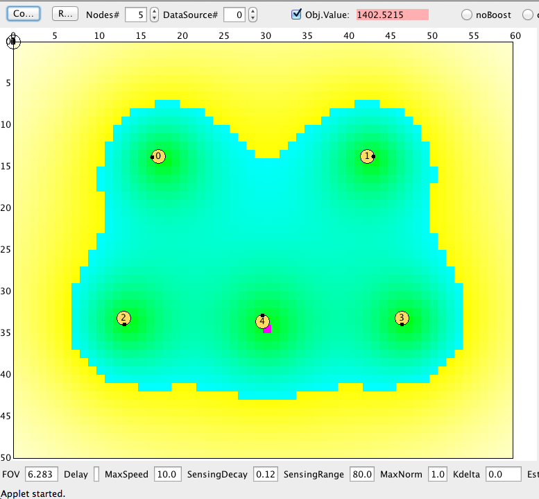
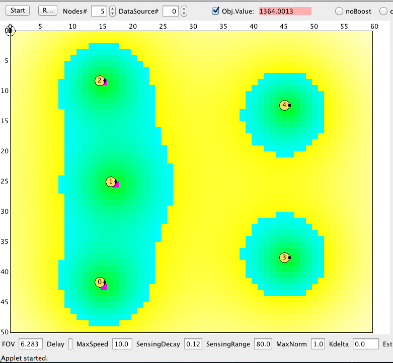
(a) Gradient-based algorithm; optimal obj.function = 1388.1 (b) Voronoi patition; optimal obj. function = 1346.5

Figure 1: Comparison between two methods used in a coverage control problem

II Problem Formulation and Distributed Optimization Solution

We begin by reviewing the general setting for a large number of multi-agent control and optimization problems and subsequently concentrate on the optimal coverage control problem. A mission space $\Omega\subset\mathbb{R}^{2}$ is modeled as a non-self-intersecting polygon, i.e., a polygon such that any two non-consecutive edges do not intersect. For any $x\in\Omega$, the function $R(x):\Omega\rightarrow\mathbb{R}$ describes some a priori information associated with $\Omega$. When the problem is to detect random events that may take place in $\Omega$, this function captures an a priori estimate of the frequency of such event occurrences and is referred to as an event density satisfying $R(x)\geq 0$ for all $x\in\Omega$ and $\int_{\Omega}R(x)dx<\infty$. The mission space may contain obstacles modeled as $m$ non-self-intersecting polygons denoted by $M_{j}$, $j=1,\ldots,m$ which block the movement of agents. The interior of $M_{j}$ is denoted by $\mathring{M_{j}}$ and the overall feasible space is $F=\Omega\setminus(\mathring{M_{1}}\cup\ldots\cup\mathring{M_{m}})$, i.e., the space $\Omega$ excluding all interior points of the obstacles. There are $N$ agents in the mission space and their positions at time $t$ are defined by $s_{i}(t)$, $i=1,\ldots,N$ with an overall position vector $\mathbf{s}(t)=(s_{1}(t),\ldots,s_{N}(t))$. Figure. 2 shows a mission space with two obstacles and an agent located at $s_{i}$. The agents may communicate with each other, but there is generally a limited communication range so that it is customary to represent such a system as a network of nodes with a link $(i,j)$ defined so that nodes $i,j$ can communicate directly with each other. This limited communication and the overall cost associated with it are major motivating factors for developing distributed schemes to allow agents to operate so as to optimally achieve a given objective with each acting as autonomously as possible.

In a coverage control problem (e.g., [9],[7],[3]), the agents are sensor nodes. We assume that each such node has a bounded sensing range captured by the sensing radius $\delta_{i}$. Thus, the sensing region of node $i$ is $\Omega_{i}=\{x:d_{i}(x)\leq\delta_{i}\}\text{ where }d_{i}(x)=\|x-s_{i}(t)\|$. The presence of obstacles inhibits the sensing ability of a node, which motivates the definition of a visibility set $V(s_{i})\subset F$ (we omit the explicit dependence of $s_{i}$ on $t$ for notational simplicity). A point $x\in F$ is visible from $s_{i}\in F$ if the line segment defined by $x$ and $s_{i}$ is contained in $F$, i.e., $[\lambda x+(1-\lambda)s_{i}]\in F$ for all $\lambda\in[0,1]$, and $x$ can be sensed, i.e. $x\in\Omega_{i}$. Then, $V(s_{i})=\Omega_{i}\cap\{x:$ $[\lambda x+(1-\lambda)s_{i}]\in F\}$ is a set of points in $F$ which are visible from $s_{i}$. We also define $\bar{V}(s_{i})=F\setminus V(s_{i})$ to be the invisibility set (e.g., the grey area in Fig. 2).

A sensing model for any node $i$ is given by the probability that $i$ detects an event occurring at $x\in V(s_{i})$, denoted by $p_{i}(x,s_{i})$. We assume that $p_{i}(x,s_{i})$ is expressed as a function of $d_{i}(x)=\|x-s_{i}\|$ and is monotonically decreasing and differentiable in $d_{i}(x)$. An example of such a function is $p_{i}(x,s_{i})=p_{0i}e^{-\lambda_{i}\|x-s_{i}\|}$. For points that are invisible by node $i$, the detection probability is zero. Thus, the overall sensing detection probability is denoted as $\hat{p}_{i}(x,s_{i})$ and defined as

$${}\hat{p}_{i}(x,s_{i})=\begin{cases}p_{i}(x,s_{i})&\text{if}\quad x\in V(s_{i})\\ 0&\text{if}\quad x\in\bar{V}(s_{i})\end{cases}$$ (1)

Note that $\hat{p}_{i}(x,s_{i})$ is not a continuous function of $s_{i}$. We may now define the joint detection probability that an event at $x\in\Omega$ is detected by at least one of the $N$ cooperating nodes in the network:

$${}P(x,\mathbf{s})=1-\prod_{i=1}^{N}[1-\hat{p}_{i}(x,s_{i})]$$ (2)

where we have assumed that detection events by nodes are independent. Finally, assuming that $R(x)=0$ for $x\notin F$, we define the optimal coverage control problem to maximize $H(\mathbf{s})$, where

$${}\begin{split}H(\mathbf{s})&=\int_{F}R(x)P(x,\mathbf{s})dx\\ s.t.\quad s_{i}&\in F,i=1,\ldots,N\end{split}$$ (3)

Thus, we seek to control the node position vector $\mathbf{s}=(s_{1},\ldots,s_{N})$ so as to maximize the overall joint detection probability of events taking place in the environment. Note that this is a nonlinear, generally nonconvex, optimization problem and the objective function $H(\mathbf{s})$ cannot be expressed in an additive form such as $\sum_{i=1}^{N}H_{i}(\mathbf{s})$.

As already mentioned, it is highly desirable to develop distributed optimization algorithms to solve (3) so as to $(i)$ limit costly communication among nodes (especially in wireless settings where it is known that communication consumes most of the energy available at each node relative to sensing or computation tasks) and $(ii)$ impart robustness to the system as a whole by avoiding single-point-of-failure issues. Towards this goal, a distributed gradient-based algorithm was developed in [9] based on the iterative scheme:

$${}s_{i}^{k+1}=s_{i}^{k}+\zeta_{k}\frac{\partial H(\mathbf{s})}{\partial s_{i}^{k}},\text{ \ }k=0,1,\ldots$$ (4)

where the step size sequence $\{{\zeta_{k}\}}$ is appropriately selected (see [14]) to ensure convergence of the resulting node trajectories. If nodes are mobile, then (4) can be interpreted as a motion control scheme for the $i$th node. In general, a solution through (4) can only lead to a local maximum and it is easy to observe that many such local maxima result in poor performance [9] (we will show such examples in Section V).

Our approach in what follows is to first show that $H(\mathbf{s})$ can be decomposed into a “local objective function” $H_{i}(\mathbf{s})$ and a function independent of $s_{i}$ so that node $i$ can locally evaluate its partial derivative with respect to its own controllable position through $H_{i}(\mathbf{s})$ alone. Our idea then is to alter $H_{i}(\mathbf{s})$ after a local optimum is attained when $\frac{\partial H_{i}(\mathbf{s})}{\partial s_{i}}=0$, and to define a new objective function $\hat{H}_{i}(\mathbf{s})$. By doing so, we force $\frac{\partial\hat{H}_{i}(\mathbf{s})}{\partial s_{i}}\neq 0$, therefore, node $i$ can “escape” the local optimum and explore the rest of the mission space in search of a potentially better equilibrium point. Because of the structure of $\frac{\partial H_{i}(\mathbf{s})}{\partial s_{i}}$ and the insights it provides, however, rather than explicitly altering $H_{i}(\mathbf{s})$ we instead alter $\frac{\partial H_{i}(\mathbf{s})}{\partial s_{i}}$ through what we refer to in Section IV as a boosting function.

III Local Objective Functions for Distributed Gradient-based Algorithms

We begin by defining $B_{i}$ to be a set of nodes with respect to $i$:

$$B_{i}=\{k:\|s_{i}-s_{k}\|<2\delta_{i},\text{ }k=1,\ldots N,\text{ }k\neq i\}$$ (5)

Clearly, this set includes all nodes $k$ whose sensing region $\Omega_{k}$ has a nonempty intersection with $\Omega_{i}$, the sensing region of node $i$. Accordingly, given that there is a total number of $N$ nodes, we define a complementary set $C_{i}$

$$C_{i}=\{k:k\notin B_{i},\text{ }k=1,\ldots N,\text{ }k\neq i\}$$ (6)

In addition, let $\Phi_{i}(x)$ denote the joint probability that a point $x\in\Omega$ is not detected by any neighbor node of $i$, defined as

$${}\Phi_{i}(x)=\prod_{k\in B_{i}}[1-\hat{p}_{k}(x,s_{k})]$$ (7)

Similarly, let $\bar{\Phi}_{i}(x)$ denote the probability that a point $x\in\Omega$ is not covered by nodes in $C_{i}$:

$$\bar{\Phi}_{i}(x)=\prod_{j\in C_{i}}[1-\hat{p}_{j}(x,s_{j})]$$ (8)

The following theorem establishes the decomposition of $H(\mathbf{s})$ into a function dependent on $s_{i}$, for any $i=1,\ldots,N$, and one dependent on all other node positions except $s_{i}$.

Theorem 1

The objective function $H(\mathbf{s})$ can be written as:

$$H(\mathbf{s})=H_{i}(\mathbf{s})+\tilde{H}(\bar{\mathbf{s}}_{i})$$ (9)

for any $i=1,\ldots,N$, where $\bar{\mathbf{s}}_{i}=(s_{1},\ldots,s_{i-1},s_{i+1},\ldots,s_{N})$, and

$$H_{i}(\mathbf{s}) =\int_{V(s_{i})}R(x)\Phi_{i}(x)p_{i}(x,s_{i})dx$$

$$\tilde{H}(\bar{\mathbf{s}}_{i}) =\int_{F}R(x)\{1-\prod_{k=1,k\neq i}^{N}[1-\hat{p}_{k}(x,s_{k})]\}dx$$

Proof: Since $F=V(s_{i})\cup\bar{V}(s_{i})$ and $V(s_{i})\cap\bar{V}(s_{i})=\varnothing$, we can rewrite $H(\mathbf{s})$ in (3) as the sum of two integrals:

$${}H(\mathbf{s})=\int_{V(s_{i})}R(x)P(x,\mathbf{s})dx+\int_{\bar{V}(s_{i})}R(x)P(x,\mathbf{s})dx$$ (10)

which we will refer to as $H_{i}^{1}(\mathbf{s})$ and $H_{i}^{2}(\mathbf{s})$, respectively. Using the definitions of $\Phi_{i}(x)$ and $\bar{\Phi}_{i}(x)$, the joint detection probability $P(x,\mathbf{s})$ in (2) can be written as

$${}P(x,\mathbf{s})=1-\Phi_{i}(x)\bar{\Phi}_{i}(x)[1-p_{i}(x)]$$ (11)

The integral domain in $H_{i}^{1}(\mathbf{s})$ is the visible set for $s_{i}$ and, from (1) we have $p_{i}(x,s_{i})\neq 0$ and $p_{j}(x,s_{j})=0$ for $j\in C_{i}$, hence, $\bar{\Phi}_{i}(x)=1$. Thus, $H_{i}^{1}(\mathbf{s})$ can be written as

$${}\begin{split}&H_{i}^{1}(\mathbf{s})=\int_{V(s_{i})}R(x)[1-\Phi_{i}(x)(1-p_{i}(x))]dx\\ &=\int_{V(s_{i})}R(x)p_{i}(x,s_{i})\Phi_{i}(x)dx+\int_{V(s_{i})}R(x)[1-\Phi_{i}(x)]dx\\ &=\int_{V(s_{i})}R(x)p_{i}(x,s_{i})\Phi_{i}(x)dx+\int_{V(s_{i})}R(x)[1-\Phi_{i}(x)\bar{\Phi}_{i}(x)]dx\end{split}$$ (12)

For the $H_{i}^{2}(\mathbf{s})$ term, the integral domain is the invisible set of $s_{i}$, which implies that $p_{i}(x,s_{i})=0$ for $x\in\bar{V}(s_{i})$. Using the form of $P(x,\mathbf{s})$ defined in (11), $H_{i}^{2}(\mathbf{s})$ can be written as

$${}H_{i}^{2}(\mathbf{s})=\int_{\bar{V}(s_{i})}R(x)[1-\Phi_{i}(x)\bar{\Phi}_{i}(x)]dx$$ (13)

Combining (12) and (13) and merging the second integral in (12) with the integral in (13), we obtain:

$$\begin{split}H(\mathbf{s})&=\int_{V(s_{i})}R(x)\Phi_{i}(x)p_{i}(x,s_{i})dx+\int_{F}R(x)[1-\Phi_{i}(x)\bar{\Phi}_{i}(x)]dx\\ &=\int_{V(s_{i})}R(x)\Phi_{i}(x)p_{i}(x,s_{i})dx\\ &+\int_{F}R(x)\big{[}1-\prod_{k=1,k\neq i}^{N}[1-\hat{p}_{k}(x,s_{k})]\big{]}dx\end{split}$$

The first term is dependent on $s_{i}$, while the second term is independent of $s_{i}$ in both integrand and integral domain. Using $\bar{\mathbf{s}}_{i}=(s_{1},\ldots,s_{i-1},s_{i+1},\ldots,s_{N})$ to denote a vector of all node positions except $i$, we define $H_{i}(\mathbf{s})$ and $\tilde{H}(\bar{\mathbf{s}}_{i})$ as

$$H_{i}(\mathbf{s}) =\int_{V(s_{i})}R(x)\Phi_{i}(x)p_{i}(x,s_{i})dx$$

$$\tilde{H}(\bar{\mathbf{s}}_{i}) =\int_{F}R(x)\{1-\prod_{k=1,k\neq i}^{N}[1-\hat{p}_{k}(x,s_{k})]\}dx$$

and the result follows. $\blacksquare$

We refer to $H_{i}(\mathbf{s})$ as the local objective function of node $i$ and observe that it depends on $V(s_{i})$, $p_{i}(x,s_{i})$, and $\Phi_{i}(x)$ which are all available to node $i$ (the latter through some communication with nodes in $B_{i}$). This result enables a distributed gradient-based optimization solution approach with each node evaluating $\frac{\partial H_{i}(\mathbf{s})}{\partial s_{i}}$. We now proceed to derive this derivative using the same method as in [15]. Based on the extension of the Leibnitz rule [16], we get

$${}\begin{split}\frac{\partial H_{i}(\mathbf{s})}{\partial s_{ix}}&=\frac{\partial}{\partial s_{ix}}\int_{V(s_{i})}R(x)\Phi_{i}(x)p_{i}(x,s_{i})dx\\ &=\int_{V(s_{i})}R(x)\Phi_{i}(x)\frac{\partial p_{i}(x,s_{i})}{\partial s_{ix}}dx\\ &+\int_{\partial V(s_{i})}R(x)\Phi_{i}(x)p_{i}(x,s_{i})(u_{x}dx_{y}-u_{y}dx_{x})\end{split}$$ (14)

where ($u_{x},u_{y}$) illustrates the “velocity” vector at a boundary point $x=(x_{x},x_{y})$ of $V(s_{i})$. The first term, denoted by $E_{ix}$, is

$${}\begin{split}E_{ix}&=\int_{V(s_{i})}R(x)\Phi_{i}(x)\frac{\partial p_{i}(x,s_{i})}{\partial s_{ix}}dx\\ &=\int_{V(s_{i})}R(x)\Phi_{i}(x)\left[-\frac{dp_{i}(x,s_{i})}{dd_{i}(x)}\right]\frac{(x-s_{i})_{x}}{d_{i}(x)}dx\end{split}$$ (15)

where $(x-s_{i})_{x}$ is the $x$ component of the vector $(x-s_{i})$. Similarly, we can obtain an integral $E_{iy}$ with $(x-s_{i})_{y}$ in place of $(x-s_{i})_{x}$.

Let $E_{i}=(E_{ix},E_{iy})$. The integrand of $E_{i}$ can be viewed as a weighted normalized direction vector $\frac{(x-s_{i})}{d_{i}(x)}$ connecting $s_{i}$ to $x\in F$ where $x$ is visible by the $i$th node. This weight is defined as

$${}w_{1}(x,\mathbf{s})=-R(x)\Phi_{i}(x)\frac{dp_{i}(x,s_{i})}{dd_{i}(x)}$$ (16)

Observe that $w_{1}(x,\mathbf{s})\geq 0$ because $\frac{dp_{i}(x,s_{i})}{dd_{i}(x)}<0$ since $p_{i}(x,s_{i})$ is a decreasing function of $d_{i}$.

Next, we evaluate the second term in (14), referred to as $E_{b}$. This evaluation is more elaborate and requires some additional notation (see Fig. 2). Let $v$ be a reflex vertex(definition can be found in [9]) of an obstacle and let $x\in F$ be a point visible from $v$. A set of points $I(v,x)$, which is a ray starting from $v$ and extending in the direction of $v-x$, is defined by

$${}I(v,x)=\{q\in V(v):q=\lambda v+(1-\lambda)x,\lambda>1\}$$ (17)

The ray intersects the boundary of $F$ at an impact point. The line from $v$ to the impact point is a $I(v,x)$.

An anchor of $s_{i}$ is a reflex vertex $v$ such that it is visible from $s_{i}$ and $I(v,s_{i})$ defined in (17) is not empty. Denote the anchors of $s_{i}$ by $v_{ij}$, $j=1,\dots,Q(s_{i})$, where $Q(s_{i})$ is the number of anchors of $s_{i}$. An impact point of $v_{ij}$, denoted by $V_{ij}$, is the intersection of $I(v_{ij},s_{i})$ and $\partial F$. As an example, in Fig. 2, $v_{i1}$, $v_{i2}$, $v_{i3}$ are anchors of $s_{i}$, and $V_{i1}$, $V_{i2}$, $V_{i3}$ are the corresponding impact points. Let $D_{ij}=\|s_{i}-v_{ij}\|$ and $d_{ij}=\|V_{ij}-v_{ij}\|$. Define $\theta_{ij}$ to be the angle formed by $s_{i}-v_{ij}$ and the $x$-axis, which satisfies $\theta_{ij}\in[0,\pi/2]$, that is, $\theta_{ij}=arctan\frac{|s_{i}-v_{ij}|_{y}}{|s_{i}-v_{ij}|_{x}}$.

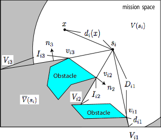
Figure 2: Mission space with two polygonal obstacles

Using this notation, a detailed derivation of the second term in (14) may be found in [15] with the final result being:

$${}\begin{split}&E_{bx}=\\ &\sum_{j\in\Gamma_{i}}sgn(n_{jx})\frac{sin\theta_{ij}}{D_{ij}}\int_{0}^{z_{ij}}R(\rho_{ij}(r))\Phi_{i}(\rho_{ij}(r))p_{i}(\rho_{ij}(r),s_{i})rdr\end{split}$$ (18)

where $\Gamma_{i}=\{j:D_{ij}<\delta_{i},j=1,\ldots,Q(s_{i})\}$; $z_{ij}=\min(d_{ij},\delta_{i}-D_{ij})$ and $\rho_{ij}(r)$ is the Cartesian coordinate of a point on $I_{ij}$ which is a distance $r$ from $v_{ij}$:

$$\rho_{ij}(r)=(V_{ij}-v_{ij})\frac{r}{d_{ij}}+v_{ij}$$ (19)

In the same way, we can also obtain $E_{by}$. Note that $E_{b}=(E_{bx},E_{by})$ is the gradient component in (14) due to points on the boundary $\partial V(s_{i})$. In particular, for each boundary, this component attracts node $i$ to move in a direction perpendicular to the boundary and pointing towards $V(s_{i})$.   We can see in (18) that every point $x$ written as $\rho_{ij}(r)$ in the integrand has an associated weight which we define as $w_{2}(x,\mathbf{s})$:

$${}w_{2}(x,\mathbf{s})=R(x)\Phi_{i}(x)p_{i}(x,s_{i})$$ (20)

and observe that $w_{2}(x,\mathbf{s})\geq 0$, as was the case for $w_{1}(x,\mathbf{s})$. Combining (15) and (18) we finally obtain the derivative of $H_{i}(\mathbf{s})$ with respect to $s_{i}$:

$${}\begin{split}&\frac{\partial{H_{i}(\mathbf{s})}}{\partial{s_{ix}}}=\int_{V(s_{i})}R(x)\prod_{k\in B_{i}}[1-\hat{p}_{k}(x,s_{k})]\frac{dp_{i}(x,s_{i})}{dd_{i}(x)}\frac{(s_{i}-x)_{x}}{d_{i}(x)}dx+\\ &\sum_{j\in\Gamma_{i}}sgn(n_{jx})\frac{sin\theta_{ij}}{D_{ij}}\int_{0}^{z_{ij}}R(\rho_{ij}(r))\Phi_{i}(\rho_{ij})(r)p_{i}(\rho_{ij}(r),s_{i})rdr\end{split}$$ (21)

$${}\begin{split}&\frac{\partial{H_{i}(\mathbf{s})}}{\partial{s_{iy}}}=\int_{V(s_{i})}R(x)\prod_{k\in B_{i}}[1-\hat{p}_{k}(x,s_{k})]\frac{dp_{i}(x,s_{i})}{dd_{i}(x)}\frac{(s_{i}-x)_{y}}{d_{i}(x)}dx+\\ &\sum_{j\in\Gamma_{i}}sgn(n_{jy})\frac{cos\theta_{ij}}{D_{ij}}\int_{0}^{z_{ij}}R(\rho_{ij}(r))\Phi_{i}(\rho_{ij})(r)p_{i}(\rho_{ij}(r),s_{i})rdr\end{split}$$ (22)

We observe that $\frac{\partial{H_{i}(\mathbf{s})}}{\partial{s_{ix}}}$, $\frac{\partial{H_{i}(\mathbf{s})}}{\partial{s_{iy}}}$ in (21)-(22) are the same as $\frac{\partial{H(\mathbf{s})}}{\partial{s_{ix}}}$, $\frac{\partial{H(\mathbf{s})}}{\partial{s_{iy}}}$, the partial derivatives of the original objective function ${H(\mathbf{s})}$ which was derived in [15]. In other words, $\frac{\partial{H(\mathbf{s})}}{\partial{s_{i}}}=\frac{\partial{H_{i}(\mathbf{s})}}{\partial{s_{i}}}$, confirming (as expected) that the local objective function $H_{i}(\mathbf{s})$ is sufficient to provide the required derivative for a distributed gradient-based algorithm using (4). As pointed out in [15], the derivation of (21)-(22) excludes pathological cases where $s_{i}$ coincides with a reflex vertex, a polygonal inflection, or a bitangent, where ${H(\mathbf{s})}$ is generally not differentiable.

We can now use the weight definitions (16) and (20) in (21) and (22) to obtain the following form of the local derivative evaluated by node $i$:

$${}\begin{split}\frac{\partial{H_{i}(\mathbf{s})}}{\partial{s_{ix}}}=&\int_{V(s_{i})}w_{1}(x,\mathbf{s})\frac{(x-s_{i})_{x}}{d_{i}(x)}dx\\ +&\sum_{j\in\Gamma_{i}}sgn(n_{jx})\frac{sin\theta_{ij}}{D_{ij}}\int_{0}^{z_{ij}}w_{2}(\rho_{ij}(r),s_{i})rdr\end{split}$$ (23)

$${}\begin{split}\frac{\partial{H_{i}(\mathbf{s})}}{\partial{s_{iy}}}=&\int_{V(s_{i})}w_{1}(x,\mathbf{s})\frac{(x-s_{i})_{y}}{d_{i}(x)}dx\\ +&\sum_{j\in\Gamma_{i}}sgn(n_{jy})\frac{cos\theta_{ij}}{D_{ij}}\int_{0}^{z_{ij}}w_{2}(\rho_{ij}(r),s_{i})rdr\end{split}$$ (24)

We can see that the essence of each derivative is captured in the weights $w_{1}(x,\mathbf{s}),$ $w_{2}(x,\mathbf{s})$. In the first integral, $w_{1}(x,\mathbf{s})$ controls the mechanism through which node $i$ is attracted to different points $x\in V(s_{i})$ through $\frac{(x-s_{i})}{d_{i}(x)}$. If obstacles are present, then $w_{2}(x,\mathbf{s})$ in the second integral controls the attraction that boundary points exert on node $i$ with the geometrical features of the mission space contributing through $n_{jx}$, $n_{jy}$, $\theta_{ij}$, and $D_{ij}$ in (23)-(24). This viewpoint motivates the boosting function approach described next.

IV The Boosting Function Approach

As defined in (3), this nonlinear, generally nonconvex, optimization problem may have multiple local optima to which a gradient-based algorithm may converge. When we apply a distributed optimization algorithm based on $\frac{\partial{H_{i}(\mathbf{s})}}{\partial{s_{i}}}$ as described above, any equilibrium point is characterized by $\frac{\partial{H_{i}(\mathbf{s})}}{\partial{s_{i}}}=0$. Since node $i$ controls its position based on its local objective function ${H_{i}(\mathbf{s})}$, a simple way to “escape” a local optimum ${\mathbf{s}}^{1}$ is to alter ${H_{i}(\mathbf{s})}$ by replacing it with some ${\hat{H}_{i}(\mathbf{s})\neq H_{i}(\mathbf{s})}$ thus forcing $\left.\frac{\partial{\hat{H}_{i}(\mathbf{s})}}{\partial{s_{i}}}\right|_{s_{i}^{1}}\neq 0$ and inducing the node to explore the rest of the mission space for potentially better equilibria. Subsequently, when a new equilibrium is reached with node $i$ at $\tilde{s}_{i}^{1}\neq s_{i}^{1}$ and $\left.\frac{\partial{\hat{H}_{i}(\mathbf{s})}}{\partial{s_{i}}}\right|_{\tilde{s}_{i}^{1}}=0$, we can revert to ${H_{i}(\mathbf{s})}$, which, in turn will force $\left.\frac{\partial{H_{i}(\mathbf{s})}}{\partial{s_{i}}}\right|_{\tilde{s}_{i}^{1}}\neq 0$ and the node will seek a new equilibrium at $s_{i}^{2}$.

Selecting the proper ${\hat{H}_{i}(\mathbf{s})}$ to temporarily replace ${H_{i}(\mathbf{s})}$ is not a simple process. However, focusing on $\frac{\partial{H_{i}(\mathbf{s})}}{\partial{s_{i}}}$ instead of ${H_{i}(\mathbf{s})}$ is much simpler due to the nature of the derivatives we derived in (23)-(24). In particular, the effect of altering ${H_{i}(\mathbf{s})}$ can be accomplished by transforming the weights $w_{1}(x,\mathbf{s})$, $w_{2}(x,\mathbf{s})$ in (23)-(24) by “boosting” them in a way that forces $\frac{\partial{H_{i}(\mathbf{s})}}{\partial{s_{i}}}=0$ at a local optimum to become nonzero. The net effect is that the attraction exerted by some points $x\in F$ on $s_{i}$ is “boosted” so as to promote exploration of the mission space by node $i$ in search of better optima.

In contrast to various techniques which aim at randomly perturbing controllable variables away from a local optimum (e.g., simulated annealing), this approach provides a systematic mechanism for accomplishing this goal by exploiting the structure of the specific optimization problem reflected through the form of the derivatives (23)-(24). Specifically, it is clear from these expressions that this can be done by assigning a higher weight (i.e., boosting) to directions in the mission space that provide greater opportunity for exploration and, ultimately “better coverage”. To develop such a systematic approach, we define transformations of the weights $w_{1}(x,s_{i})$, $w_{2}(x,\mathbf{s})$ for interior points and for boundary points respectively as follows:

$$\hat{w}_{1}(x,\mathbf{s}) =g_{i}(w_{1}(x,\mathbf{s}))$$ (25)

$$\hat{w}_{2}(x,\mathbf{s}) =h_{i}(w_{2}(x,\mathbf{s}))$$ (26)

where $g_{i}(\cdot)$ and $h_{i}(\cdot)$ are functions of the original weights $w_{1}(x,\mathbf{s})$ and $w_{2}(x,\mathbf{s})$ respectively. We refer to $g_{i}(\cdot)$ and $h_{i}(\cdot)$ as boosting functions for node $i=1,\ldots,N$. Note that these may be node-dependent and that each node may select the time at which this boosting is done, independent from other nodes. In other words, the boosting operation may also be implemented in distributed fashion, in which case we refer to this process at node $i$ as self-boosting.

In the remainder of this paper, we concentrate on functions $g_{i}(\cdot)$ and $h_{i}(\cdot)$ which have the form

$${}\hat{w}_{1}(x,\mathbf{s}) =\alpha_{i1}(x,\mathbf{s})w_{1}(x,\mathbf{s})+\beta_{i1}(x,\mathbf{s})$$ (27)

$${}\hat{w}_{2}(x,\mathbf{s}) =\alpha_{i2}(x,\mathbf{s})w_{2}(x,\mathbf{s})+\beta_{i2}(x,\mathbf{s})$$ (28)

where $\alpha_{i1}(x,\mathbf{s})$, $\beta_{i1}(x,\mathbf{s})$, $\alpha_{i2}(x,\mathbf{s})$, and $\beta_{i2}(x,\mathbf{s})$ are functions dependent on the point $x$ and the node position vector $\mathbf{s}$ in general. We point out that although the form of (27)-(28) is linear, the functions $\alpha_{ij}(x,\mathbf{s})$, $\beta_{ij}(x,\mathbf{s})$, $j=1,2$, $i=1,\ldots,N$ are generally nonlinear in their arguments.

To keep notation simple, let us concentrate on a single node $i$ and omit the subscript $i$ in $\alpha_{ij}(x,\mathbf{s})$, $\beta_{ij}(x,\mathbf{s})$ above. By replacing $w_{1}(x,\mathbf{s})$, $w_{2}(x,\mathbf{s})$ with $\hat{w}_{1}(x,s_{i})$, $\hat{w}_{2}(x,s_{i})$ respectively, we obtain the boosted derivative $\frac{\partial{\hat{H}(\mathbf{s})}}{\partial s_{i}}$ as follows

$${}\begin{split}\frac{\partial{\hat{H}(\mathbf{s})}}{\partial{s_{ix}}}=&\int_{V(s_{i})}\alpha_{1}(x,\mathbf{s})w_{1}(x,\mathbf{s})\frac{(x-s_{i})_{x}}{d_{i}(x)}dx\\ +&\int_{V(s_{i})}\beta_{1}(x,\mathbf{s})\frac{(x-s_{i})_{x}}{d_{i}(x)}dx\\ +&\sum_{j\in\Gamma_{i}}sgn(n_{jx})\frac{sin\theta_{ij}}{D_{ij}}\int_{0}^{z_{ij}}\alpha_{2}(x,\mathbf{s})w_{2}(x,\mathbf{s})rdr\\ +&\sum_{j\in\Gamma_{i}}sgn(n_{jx})\frac{sin\theta_{ij}}{D_{ij}}\int_{0}^{z_{ij}}\beta_{2}(x,\mathbf{s})rdr\end{split}$$ (29)

$\frac{\partial{\hat{H}(\mathbf{s})}}{\partial{s_{iy}}}$ can be obtained in a similar way. Obviously, the boosting process (27)-(28) actually changes the objective function $H(\mathbf{s})$. Thus, when a new equilibrium is reached in the boosted derivative phase of system operation, it is necessary to revert to the original objective function by setting $\alpha_{1}(x,\mathbf{s})=\alpha_{2}(x,\mathbf{s})=1$ and $\beta_{1}(x,\mathbf{s})=$ $\beta_{2}(x,\mathbf{s})=0$.

We summarize the boosting process as follows. Initially, node $i$ uses (23)-(24) until an equilibrium ${\mathbf{s}}^{1}$ is reached at time $\tau^{1}$ and nodes communicate their positions to each other.

1. At $t=\tau^{1}$, evaluate $H{(\mathbf{s}(\tau^{1}))}$ and set ${\mathbf{s}}^{\ast}={\mathbf{s}}^{1}$ and $H^{\ast}{=}H{(\mathbf{s}(\tau^{1}))}$. Then, apply boosting functions (27)-(28), evaluate (29), and iterate on the controllable node position using (4). Set $BIt=0$. $BIt$ is short for the Boosted iteration, which is a counter for iteration needed for a new local optima.

2. Wait until $\frac{\partial{\hat{H}(\mathbf{s})}}{\partial{s_{ix}}}=\frac{\partial{\hat{H}(\mathbf{s})}}{\partial{s_{iy}}}=0$ at time $\hat{\tau}^{1}>\tau^{1}$.

3. At $t=\hat{\tau}^{1}$, set $\alpha_{1}(x,\mathbf{s})=\alpha_{2}(x,\mathbf{s})=1$ and $\beta_{1}(x,\mathbf{s})=$ $\beta_{2}(x,\mathbf{s})=0$ and revert to $\frac{\partial{H_{i}(\mathbf{s})}}{\partial{s_{i}}}$.

4. Wait until $\frac{\partial{H(\mathbf{s})}}{\partial{s_{ix}}}=\frac{\partial H{(\mathbf{s})}}{\partial{s_{iy}}}=0$ at time $\tau^{2}>\hat{\tau}^{1}$ and evaluate $H{(\mathbf{s}(\tau^{2}))}$, get $BIt$. If $H{(\mathbf{s}(\tau^{2}))>}H^{\ast}$, then set ${\mathbf{s}}^{\ast}={\mathbf{s}(\tau^{2})}$ and $H^{\ast}{=}H{(\mathbf{s}(\tau^{2}))}$. Otherwise, ${\mathbf{s}}^{\ast},$ $H^{\ast}$ remain unchanged (if nodes are mobile and have already been moved to ${\mathbf{s}(\tau^{2})}$, then return them to ${\mathbf{s}}^{\ast}$).

5. Either STOP, or repeat the process from the current ${\mathbf{s}}^{\ast}$ with a new boosting function to further explore the mission space for better equilibrium points.

Note that if ${\mathbf{s}}^{1}$ is a global optimum, then the boosting process simply perturbs node locations until Step 4 returns them to ${\mathbf{s}}^{1}$. The process will stop if no solution is better than $\mathbf{s}^{1}$ after trying finite boosting functions. It is also possible (due to symmetry) that there are multiple global optima, in which case $H{(\mathbf{s}(\tau^{2}))=}H{(\mathbf{s}(\tau^{1}))}$ and the new equilibrium point is equivalent to the original one.

The process above assumes that all nodes wait until they have all reached an equilibrium point ${\mathbf{s}}^{1}$ before each initiates its boosting process. However, this may also be done in a distributed function through a self-boosting process: node $i$ may apply (27)-(28) as soon as it observes $\frac{\partial{H(\mathbf{s})}}{\partial{s_{ix}}}=\frac{\partial H{(\mathbf{s})}}{\partial{s_{iy}}}=0$.

IV-A Boosting Function Selection

The selection of boosting functions generally depends on the mission space topology. For instance, it is clear that if there are no obstacles, then $\alpha_{2}(x,\mathbf{s})=1$, $\beta_{2}(x,\mathbf{s})=0$, since only the first integrals in (23)-(24) are present. In what follows, we present three families of boosting functions that we have investigated to date; each has different properties and has provided promising results.

Before proceeding, we make a few observations which guide the selection of boosting functions. First, we exclude cases such that $\alpha_{1}(x,s_{i})=\alpha_{2}(x,s_{i})=C$ independent of $x$, and $\beta_{1}(x,s_{i})=$ $\beta_{2}(x,s_{i})=0$. In such cases, the boosting effect is null, since it implies that $\frac{\partial{\hat{H}(\mathbf{s})}}{\partial{s_{i}}}=C\frac{\partial{H(\mathbf{s})}}{\partial{s_{i}}}$, which has no effect on $\frac{\partial{H(\mathbf{s})}}{\partial{s_{i}}}=0$. Second, we observe that if $\left|\beta_{1}(x,s_{i})\right|>>\alpha_{1}(x,s_{i})w_{1}(x,\mathbf{s})$, then the first integral in (29) is dominated by the second one, and the net effect is that nodes tend to be attracted to a single point (their center of mass) instead of exploring the mission space. The third observation is more subtle. The first term of (23) contains information on points of the visible set $V(s_{i})$, which is generally more valuable (i.e., more points in $V(s_{i})$) than the information in the second term related to the boundary points in $\Gamma_{i}$ (except, possibly, for unusual obstacle configurations). Thus, a boosting function should ensure that the first integral in (23) dominates the second when $\frac{\partial{H_{i}(\mathbf{s})}}{\partial{s_{i}x}}\neq 0$. In order to avoid such issues, in the sequel we limit ourselves to boosting $w_{1}(x,\mathbf{s})$ only and, therefore, we set $\alpha_{2}(x,s_{i})=1$, $\beta_{2}(x,s_{i})=0$.

IV-A1 $P$-Boosting function

In this function, we keep $\beta_{1}(x,\mathbf{s})=0$ and only concentrate on $\alpha_{1}(x,\mathbf{s})$ which we set:

$$\alpha_{1}(x,\mathbf{s})=k{P(x,\mathbf{s})}^{-\gamma}$$ (30)

where $P(x,\mathbf{s})$ is the joint detection probability defined in (2), $\gamma$ is a positive integer parameter and $k$ is a gain parameter. Thus, the boosted derivative associated with this $P$-boosting function is

$${}\begin{split}\frac{\partial{\hat{H}(\mathbf{s})}}{\partial{s_{ix}}}=&\int_{V(s_{i})}k{P(x,\mathbf{s})}^{-\gamma}w_{1}(x,\mathbf{s})\frac{(x-s_{i})_{x}}{d_{i}(x)}dx\\ +&\sum_{j\in\Gamma_{i}}sgn(n_{jx})\frac{sin\theta_{ij}}{D_{ij}}\int_{0}^{z_{ij}}w_{2}(x,\mathbf{s})rdr\\ \end{split}$$ (31)

The motivation for this function is similar to a method used in [9] to assign higher weights for low-coverage interior points in $V(s_{i})$, in order for nodes to explore such low coverage areas. This is consistent with the following properties of this boosting function: $({P(x,\mathbf{s})})^{-\gamma}\rightarrow\infty$ as $P(x,\mathbf{s})\rightarrow 0$, and $({P(x,\mathbf{s})})^{-\gamma}\rightarrow 1$ as $P(x,\mathbf{s})\rightarrow 1$.

IV-A2 Neighbor-Boosting function

We set $\alpha_{1}(x,\mathbf{s})=1$ and focus on $\beta_{1}(x,\mathbf{s})$. Every node applies a repelling force on each of its neighbors with the effect being monotonically decreasing with their relative distance. We define:

$$\beta_{1}(x,\mathbf{s})=\sum_{j\in B_{i}}\delta(x-s_{j})\frac{k_{j}}{\|s_{i}-x\|^{\gamma}}$$ (32)

where $k_{j}\geq 0$ is a gain parameter for $j$, $\gamma$ is a positive integer parameter, and $\delta(x-s_{j})$ is the delta function. The boosted derivative associated with this neighbor-boosting function is

$${}\begin{split}\frac{\partial{\hat{H}(\mathbf{s})}}{\partial{s_{ix}}}=&\int_{V(s_{i})}w_{1}(x,\mathbf{s})\frac{(x-s_{i})_{x}}{d_{i}(x)}dx\\ +&\sum_{j\in\Gamma_{i}}sgn(n_{jx})\frac{sin\theta_{ij}}{D_{ij}}\int_{0}^{z_{ij}}w_{2}(x,\mathbf{s})rdr\\ +&\sum_{j\in B_{i}}\frac{k_{j}}{\|s_{j}-s_{i}\|^{\gamma+1}}(s_{j}-s_{i})_{x}\end{split}$$ (33)

Note that $k_{j}$ may vary over different neighbors $j$. For instance, if some neighboring node $j$ is such that $j\notin V(s_{i})$, then we may set $k_{j}=0$.

IV-A3 $\Phi$-boosting function

This function aims at varying $\alpha_{1}(x,\mathbf{s})$ by means of $\Phi_{i}(x)$ defined in (7), which is the probability that point $x$ is not detected by neighboring nodes of $i$. $\beta_{1}(x,\mathbf{s})=0$ as well. Large $\Phi_{i}(x)$ values imply a lower coverage by neighbors, therefore higher weights are set. In particular, we define

$$\alpha_{1}(x,\mathbf{s})=k\Phi_{i}(x)^{\gamma}$$ (34)

where $k$ is a gain parameter and $\gamma$ is a positive integer parameter. The boosted derivative here is

$${}\begin{split}\frac{\partial{\hat{H}(\mathbf{s})}}{\partial{s_{ix}}}=&\int_{V(s_{i})}k\Phi_{i}(x)^{\gamma}w_{1}(x,\mathbf{s})\frac{(x-s_{i})_{x}}{d_{i}(x)}dx\\ +&\sum_{j\in\Gamma_{i}}sgn(n_{jx})\frac{sin\theta_{ij}}{D_{ij}}\int_{0}^{z_{ij}}w_{2}(x,\mathbf{s})rdr\\ &\end{split}$$ (35)

Observe that $\Phi_{i}(x)=0$ means that $x$ is well-covered by neighbors of $i$, therefore, sensor node $i$ has no incentive to move closer to this point. On the other hand, $\Phi_{i}(x)=1$ means that no neighbor covers $x$, so the boosted weight is the value of the gain $k$.

To compare the performance of the boosting function method to that of a random perturbation method, we propose a random perturbation method applied in step 1 to get (29) in the boosting process. Let $\xi_{x},\xi_{y}$ be independent random variables. The perturbed derivatives $\frac{\partial{\hat{H}(\mathbf{s})}}{\partial{s_{ix}}}$, $\frac{\partial{\hat{H}(\mathbf{s})}}{\partial{s_{iy}}}$ will be

$${}\frac{\partial{\hat{H}(\mathbf{s})}}{\partial{s_{ix}}}=\frac{\partial{H(\mathbf{s})}}{\partial{s_{ix}}}+\xi_{x}$$ (36)

$${}\frac{\partial{\hat{H}(\mathbf{s})}}{\partial{s_{iy}}}=\frac{\partial{H(\mathbf{s})}}{\partial{s_{iy}}}+\xi_{y}$$ (37)

Note that $\xi_{x}$ and $\xi_{y}$ are independently updated for each node in each iteration. Then, this random perturbation method can be performed in a distributed way.

V Simulation Results

In this section, we provide simulation examples illustrating how the objective function value in (3) is improved by using the boosting function process and how the parameter values in the boosting functions we have considered can further affect performance. Moreover, we show how the boosting method is superior to the random perturbation approach in terms of the number of iterations to a new local optimum.

Figure. 3 presents four mission spaces with different obstacle configurations (obstacles shown as blue polygons), which we refer to as “General Obstacle”, “Room Obstacle”, “Maze Obstacle” and “Narrow Obstacle” , respectively. The event density functions are uniform in all cases, i.e., $R(x)=1$. In the first three cases, there are 10 nodes shown as numbered circles while in the Narrow Obstacle case, there are only 2 nodes. The mission space is colored from dark to lighter as the joint detection probability decreases (the joint detection probability is $\geq 0.97$ for purple areas, $\geq 0.50$ for green areas, and near zero for white areas). Nodes start from the upper left corner and reach equilibrium configurations obtained by the gradient-based algorithm in [9]. The objective function values at the equilibria are shown in the captions of Figs. 3-3. It is easy to see that these deployments are sub-optimal due to the obvious imbalanced coverage. For instance, in Fig. 3, the upper and lower rightmost “rooms” are poorly covered while there are 4 nodes clustered together near the first obstacle on the left side. We expect that boosting functions can guide nodes towards exploration of poorly covered areas in the mission space, thus leading to a more balanced, possibly globally optimal, equilibrium.

First, we discuss how we select parameters for the boosting functions. For the neighbor-boosting function, we select the gain parameters $k_{j}$ in two different ways: $(i)$ the same for all neighboring nodes in a line of sight of $s_{i}$, otherwise, $k_{j}=0$:

$$k_{j}=\begin{cases}k&\text{if}\quad s_{j}\in V(s_{i}),\text{ }j\in B_{i}\\ 0&\text{otherwise}\end{cases}$$ (38)

and $(ii)$, $k_{j}=0$ for all neighboring nodes except for the closest neighbor of $s_{i}$:

$$k_{j}=\begin{cases}k&j=\text{arg }min_{k\in B_{i}}\|s_{i}-s_{k}\|\\ 0&\text{otherwise}\end{cases}$$ (39)

We define $H(\mathbf{s}^{\ast})_{1}$ and $H(\mathbf{s}^{\ast})_{2}$ to correspond to the objective function values after the boosting process for each of these two choices and have found through extensive experimentation (shown in Table. I) that $H(\mathbf{s}^{\ast})_{2}>H(\mathbf{s}^{\ast})_{1}$ for almost cases considered. In the following discussion, the second definition of $k_{j}$ is used.

We also study the effect of the parameters $\gamma$ and $k$ and have found the $\gamma$, $k$ that yield the best results for all boosting functions (shown in the captions). Table I lists results from some of our experiments. For instance, in the room case, the neighbor-boosting function with $\gamma=1$ and $k=300$ yields the largest objective value $H(\mathbf{s}^{\ast})_{2}$.

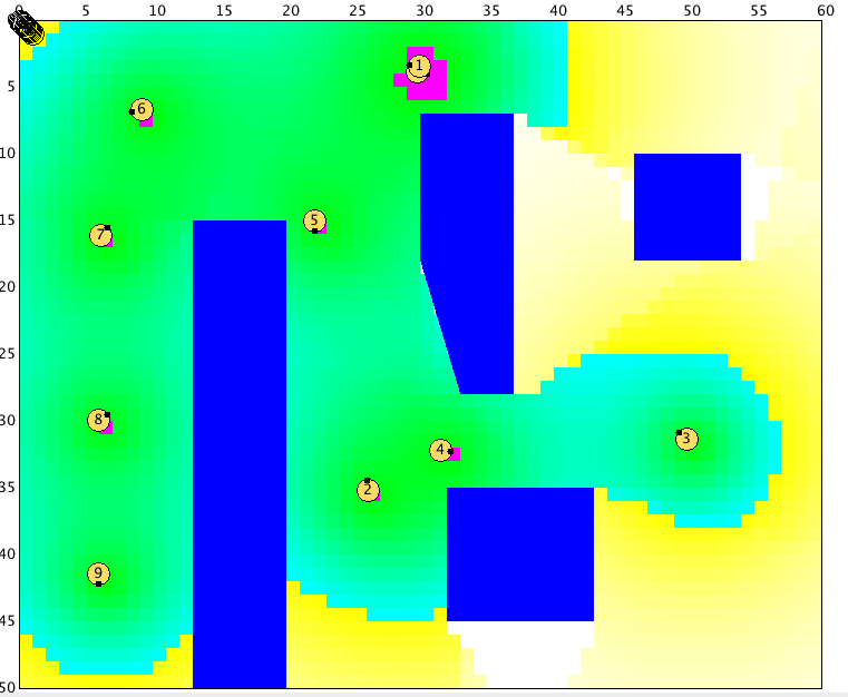
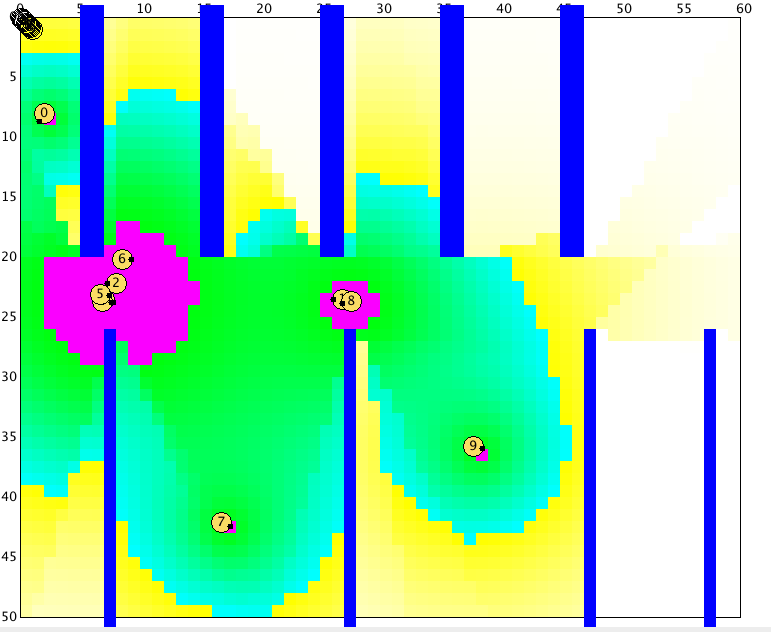
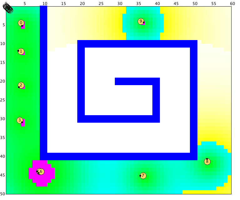
(a) General obstacle with $H(\textbf{s}_{0}^{*})=1368.3$ (b) Room obstacle with $H(\textbf{s}_{0}^{*})=1183.5$
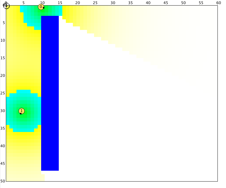
(c) Maze obstacle with $H(\textbf{s}_{0}^{*})=904.0$ (d) Narrow obstacle with $H(\textbf{s}_{0}^{*})=246.5$

Figure 3: Initial local optima in all obstacle configurations

Then, we show the results for all configurations. Figure. 4 illustrates the effects of different methods used in the general obstacle configuration. The $P$-boosting and the $\Phi$-boosting functions attain the best local optima (objective values are increased by 12%) in the smallest number of iterations. Figure. 4 shows a snapshot of a typical result using the random perturbation approach in (36)-(37). It needs about four times as many iterations as the $\Phi$-boosting function, yet converges to a worse local optimum.

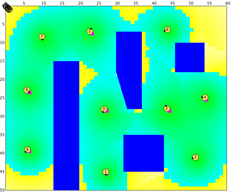
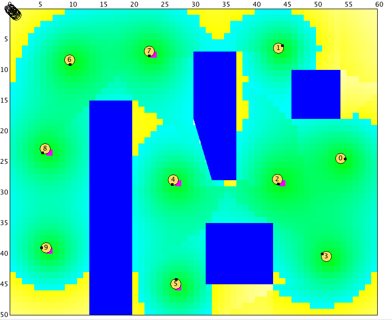
(a) $P$-boost, $\gamma=4$, $k=100$, BIt=161; $H(\textbf{s}^{*})=1533.6$ (b) Neighbor-boost, $\gamma=2$, $k=500$, BIt=390; $H(\textbf{s}^{*})=1533.3$
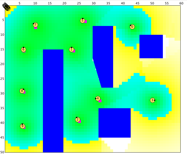
(c) $\Phi$-boost, $\gamma=2$, $k=1000$, BIt=160; $H(\textbf{s}^{*})=1533.4$ (d) Random Perturbation, BIt=653; $H(\textbf{s}^{*})=1443.9$

Figure 4: General Obstacle Configuration

Next, we consider the ”Room” obstacle case in Fig. 5. Comparing Fig. 3 with Fig. 5, the clustered nodes in Fig. 3 have spread apart and the objective value has increased. The $P$-boosting and the $\Phi$-boosting converge to better local optima (about 20% increase in the objective function value over the original one) than those resulting from the neighbor-boosting function. The random perturbation gets stuck at a worse equilibrium after more iterations than any boosting function.

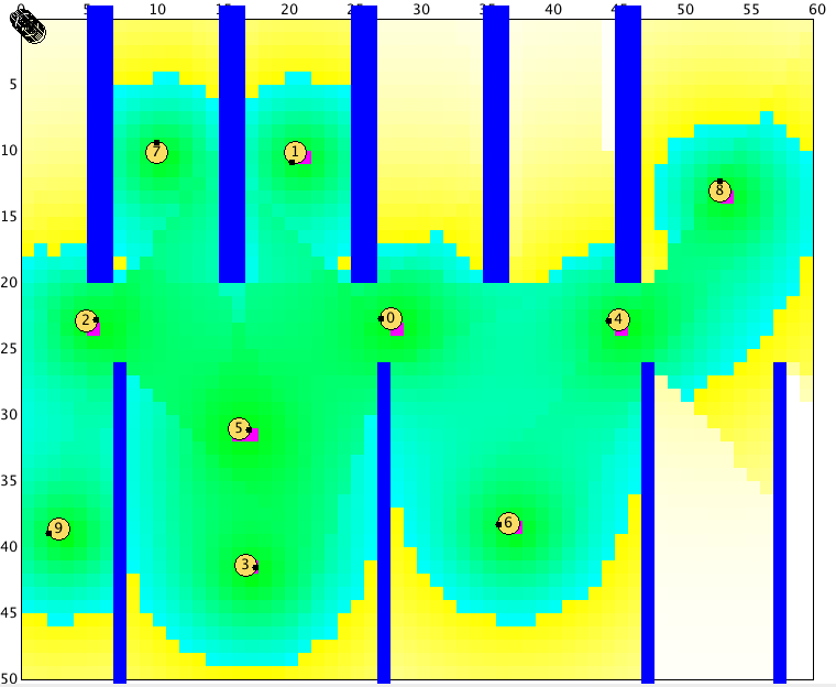
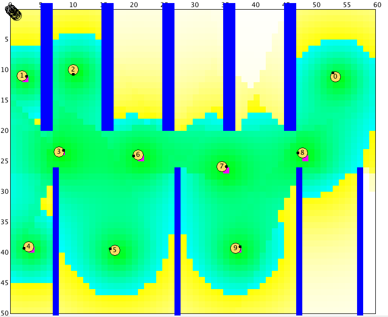
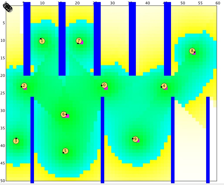
(a) $P$-boost, $\gamma=4$, $k=100$; BIt=221, $H(\textbf{s}^{*})=1419.5$ (b) Neighbor-boost, $\gamma=1$, $k=300$; BIt=364, $H(\textbf{s}^{*})=1417.1$
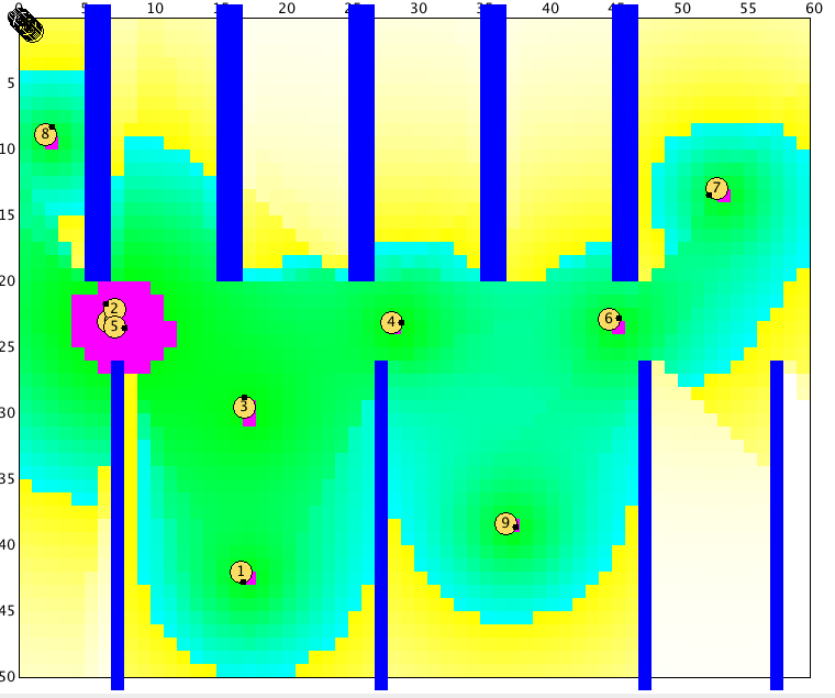
(c) $\Phi$-boost, $\gamma=1$, $k=1000$; BIt=208, $H(\textbf{s}^{*})=1419.1$ (d) Random Perturbation BIt=850; $H(\textbf{s}^{*})=1377.3$

Figure 5: Room Obstacle Configuration

Figure. 6 displays the results of boosting functions applied to the maze configuration. The $\Phi$-boosting function attains a local optimum with the highest objective function value (approximately a 44% increase in the objective function value over the original one) among all methods while the random-boosting does the worst. Figure. 7 shows results for the narrow obstacle configuration where the $P$-boosting function works the best and the objective function value is increased by 105%, from 245.3 to 502.5. Note that the neighbor-boosting function fails to escape the local optimum. This is because the repelling forces between the two nodes have no components to drive sensor nodes over the obstacle. Although the random perturbation method converges to similar results as the $\Phi$-boosting function, it requires many more iterations.

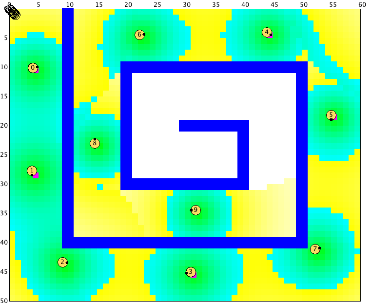
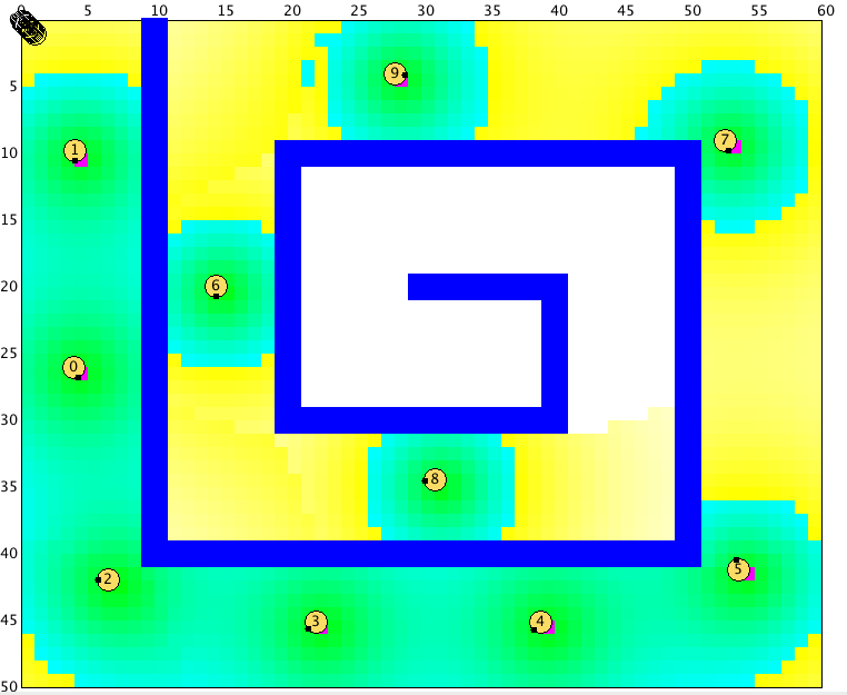
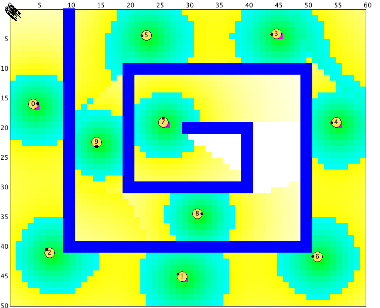
(a) $P$-boost, $\gamma=4$, $k=100$; BIt=517, $H(\textbf{s}^{*})=1180.5$ (b) Neighbor-boost,$\gamma=2$, $k=1000$; BIt=600, $H(\textbf{s}^{*})=1168.6$
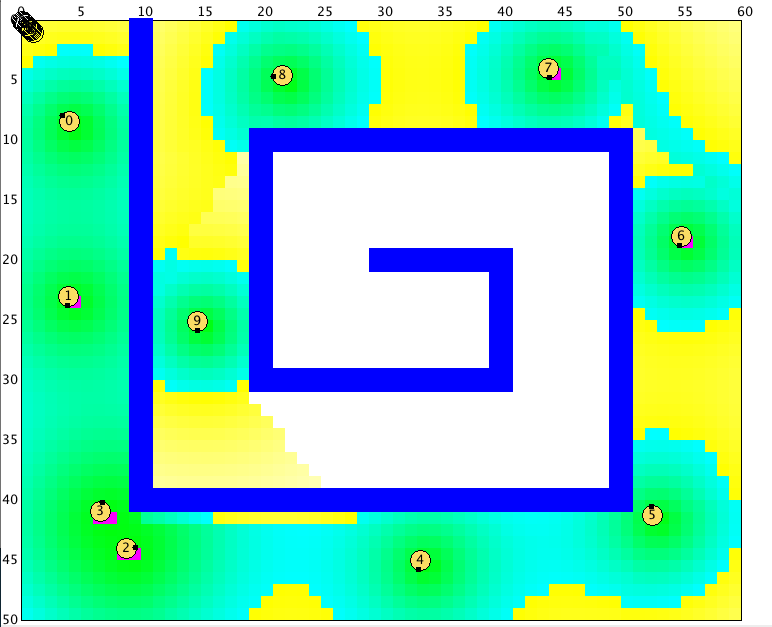
(c) $\Phi$-boost, $\gamma=2$, $k=100$; BIt=503, $H(\textbf{s}^{*})=1236.1$ (d) Random Perturbation BIt=3439; $H(\textbf{s}^{*})=1132.3$

Figure 6: Maze Obstacle Configuration

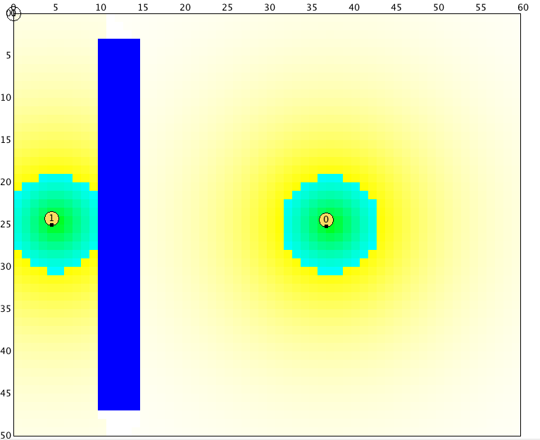
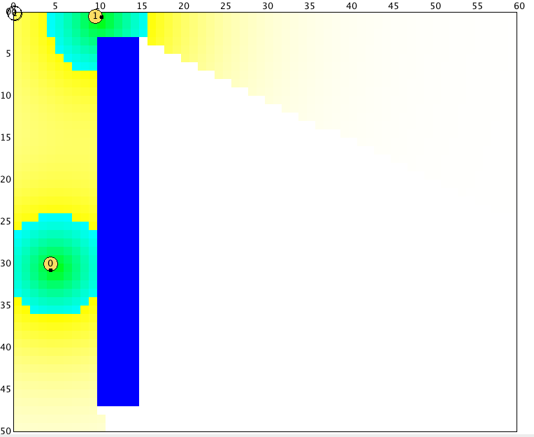
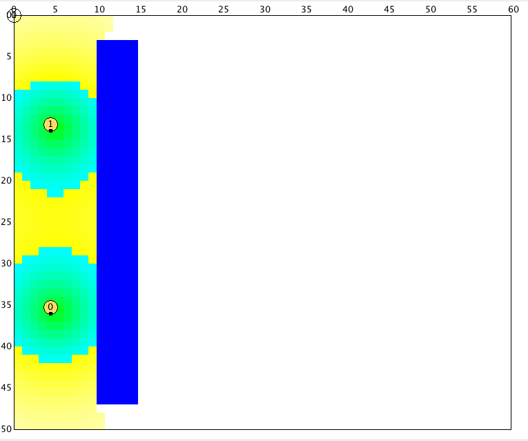
(a) $P$-boost, $\gamma=4$, $k=100$; BIt=103, $H(\textbf{s}^{*})=502.5$ (b) Neighbor-boost, $\gamma=1$, $k=300$; BIt=212; $H(\textbf{s}^{*})=246.5$
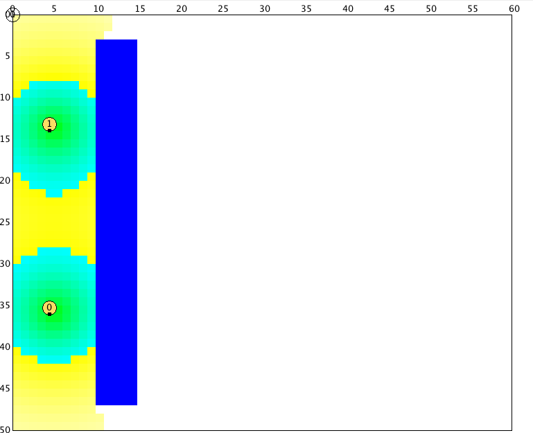
(c) $\Phi$-boost, $\gamma=2$, $k=1000$; BIt=90; $H(\textbf{s}^{*})=253.3$ (d) Random Perturbation BIt=1153; $H(\textbf{s}^{*})=253.3$

Figure 7: Narrow Obstacle Configuration

In summary, we conclude that the boosting function approach, while still not guaranteeing global optimality, provides substantial improvements in the objective function value, varying from 12% to 105%. In addition, the boosting function approach converges to an equilibrium faster and usually with a higher objective function value than the random perturbation method.

$\gamma$	$k$	Obstacle Type	$H(\textbf{s}^{*})_{1}$	$H(\textbf{s}^{*})_{2}$
1	300	General	1513.7	1470.0
2	300	General	1450.6	1451.0
2	500	General	1505.1	1533.3
2	1000	General	1446.6	1530.7
1	300	Room	1372.9	1417.1
2	300	Room	1380.8	1392.5
2	500	Room	1382.8	1395.2
2	1000	Room	1378	1380.8
1	300	Maze	1051.8	1110.3
2	300	Maze	1051.8	1133.7
2	500	Maze	1109.3	1110.5
2	1000	Maze	1133.9	1168.6
1	300	Narrow	245.3	245.3
2	300	Narrow	245.3	245.3
2	500	Narrow	245.3	245.3
2	1000	Narrow	245.3	245.3

TABLE I: The boosted objective function values by neighbor-boosting

VI Conclusions and future work

We have shown that the objective function $H(\mathbf{s})$ for the class of optimal coverage control problems in multi-agent system environments can be decomposed into a local objective function $H_{i}(\mathbf{s})$ for each node $i$ and a function independent of node $i$’s controllable position $s_{i}$. This leads to the definition of boosting functions to systematically (as opposed to randomly) allow nodes to escape from a local optimum so that the attraction exerted by some points on  a node $i$ is “boosted” to promote exploration of the mission space by $i$ in search of better optima. We have defined three families of boosting functions, and provided simulation results illustrating their effects and relative performance. Ongoing research aims at combining different boosting functions to create a “hybrid” approach and at studying self-boosting processes whereby individual nodes autonomously control their boosting in a distributed manner.

References

- [1] M. Zhu and S. Martinez, “An approximate dual subgradient algorithm for multi-agent non-convex optimization,” IEEE Transactions on Autom. Control, vol. 58, no. 6, pp. 1534–1539, 2013.
- [2] S. Meguerdichian, F. Koushanfar, M. Potkonjak, and M. Srivastava, “Coverage problems in wireless ad-hoc sensor networks,” in Proc. of 20th Annual Joint Conf. of the IEEE Computer and Commun. Societies, vol. 3, 2001, pp. 1380–1387.
- [3] J. Cortes, S. Martinez, T. Karatas, and F. Bullo, “Coverage control for mobile sensing networks,” IEEE Transactions on Robotics and Automation, vol. 20, no. 2, pp. 243–255, 2004.
- [4] L. Mihaylova, T. Lefebvre, H. Bruyninckx, K. Gadeyne, and J. D. Schutter, “Active sensing for robotics - a survey,” in Proc. 5th Int’l Conf. On Numerical Methods and Applications, 2002, pp. 316–324.
- [5] C. G. Cassandras and W. Li, “Sensor networks and cooperative control,” European Journal of Control, vol. 11, no. 4, 2005.
- [6] C. Caicedo-Nuez and M. Zefran, “A coverage algorithm for a class of non-convex regions,” in Proc. of the 47th IEEE Conf. on Decision and Control, 2008, pp. 4244–4249.
- [7] C. H. Caicedo-Nunez and M. Zefran, “Performing coverage on nonconvex domains,” in Proc. of the 2008 IEEE Conf. on Control Applic., 2008, pp. 1019–1024.
- [8] A. Breitenmoser, M. Schwager, J.-C. Metzger, R. Siegwart, and D. Rus, “Voronoi coverage of non-convex environments with a group of networked robots,” in Proc. of the 2010 IEEE International Conference on Robotics and Automation (ICRA), 2010, pp. 4982–4989.
- [9] M. Zhong and C. Cassandras, “Distributed coverage control and data collection with mobile sensor networks,” IEEE Transactions on Automatic Control, vol. 56, no. 10, pp. 2445–2455, 2011.
- [10] A. Gusrialdi, S. Hirche, T. Hatanaka, and M. Fujita, “Voronoi based coverage control with anisotropic sensors,” in Proc. of the 2008 American Control Conf., 2008, pp. 736–741.
- [11] P. J. Van Laarhoven and E. H. Aarts, Simulated annealing. Springer, 1987.
- [12] D. Bertsimas and J. Tsitsiklis, “Simulated annealing,” Statistical Science, pp. 10–15, 1993.
- [13] M. Schwager, F. Bullo, D. Skelly, and D. Rus, “A ladybug exploration strategy for distributed adaptive coverage control,” in Proc. of the IEEE International Conference on Robotics and Automation, 2008, pp. 2346–2353.
- [14] D. P. Bertsekas, Nonlinear Programming. Athena Scientific, 1995.
- [15] C. G. Cassandras and M. Zhong, “Distributed coverage control in sensor network environments with polygonal obstacles,” in Proc. of the 17th IFAC World Congress, vol. 17, no. 1, 2008, pp. 4162–4167.
- [16] H. Flanders, “Differentiation under the integral sign,” The American Mathematical Monthly, vol. 80, no. 6, pp. 615–627, 1973.