Extremum Seeking-based Iterative Learning Linear MPC

Abstract

In this work we study the problem of adaptive MPC for linear time-invariant uncertain models. We assume linear models with parametric uncertainties, and propose an iterative multi-variable extremum seeking (MES)-based learning MPC algorithm to learn on-line the uncertain parameters and update the MPC model. We show the effectiveness of this algorithm on a DC servo motor control example.

I Introduction

Model predictive control (MPC) [1] is a model-based framework for optimal control of constrained multi-variable systems. MPC is based on the repeated, receding horizon solution of a finite-time optimal control problem formulated from the system dynamics, constraints on system states, inputs, outputs, and a cost function describing the control objective. MPC has been applied to several applications such as aerospace [2],[3], automotive [4],[5], and mechatronic systems [6],[7]. Since MPC is a model-based controller, its performance inevitably depends on the quality of the prediction model used in the optimal control computation.

In contrast, extremum seeking (ES) control is a well known approach where the extremum of a cost function associated with a given process performance (under some conditions) is found without the need for detailed modeling information, see, e.g., [8, 9, 10]. Several ES algorithms (and associated stability analyses) have been proposed, [11, 9, 12, 10, 12, 8, 13, 14], and many applications of ES have been reported [15, 16, 17, 18, 19].

The idea that we introduce in this work, is that the performance of a model-based MPC controller can be combined with the robustness of a model-free ES learning algorithm for simultaneous identification and control of linear time-invariant systems with structural uncertainties. While regulation and identification are seemingly conflicting objectives, by identifying (or re-identifying) the system dynamics online and updating the MPC prediction model, the closed-loop performance may be enhanced relative to a standard MPC scheme that uses an inaccurate (or outdated) model. The optimal solution to this trade-off between identification and control is given by a dynamic program [20], which, for many applications, is computationally intractable. As a result, many suboptimal techniques and heuristics have been developed in recent years – often in a receding horizon framework which is suitable for integration with MPC.

In [21], an approximation of the dynamic program is developed for a linear input-output map with no dynamics. Approaches for more complex systems avoid dynamic programming altogether and, instead, sub-optimally trade off between inputs that excite the system and inputs that regulate the state. Excitation signals are often designed to satisfy persistency of excitation conditions. For example, a dithering signal may be added on top of the nominal control [22], although difficulties arise in determining the amplitude of the signal, and the dither indiscriminately adds noise to the process. More sophisticated schemes employ optimal input design, usually in the frequency domain, where maximizing the Fisher information matrix can be cast as a semi-definite program [23]. However, design in the frequency domain leads to difficulties with constraints that are more naturally addressed in the time domain, e.g., input (and possibly output) amplitude constraints. While the problem formulation in the time domain is highly non-convex, developing such techniques is desirable, and thus the focus of recent work [24, 25, 26, 27, 28, 29, 30, 31, 32].

In this preliminary work, we aim at proposing an alternative approach to realize an iterative learning-based adaptive MPC. We introduce an approach for a multi-variable extremum seeking (MES)-based iterative learning MPC that merges a model-based linear MPC algorithm with a model-free MES algorithm to realize an iterative learning MPC that adjusts to structured model uncertainties. This approach is an extension to the recent MPC framework reported in [33], where the author proposed to use MES with model-based nonlinear control to design learning-based adaptive controllers for a class of nonlinear systems.

The paper is organized as follows. We start the paper with some preliminaries in Section II. In Section III, we first recall the nominal MPC algorithm and then present the main result of the paper, namely, the iterative learning MPC, with a discussion of the algorithm stability. Section IV is dedicated to a DC servo-motor case study. Finally, we conclude the paper with a brief summary of the results in Section V.

II Notations and preliminaries

Throughout the paper, $\mathbb{R}$, $\mathbb{Z}_{0+}$, $\mathbb{Z}_{[i,j]}$ denote the set of real numbers, positive integers, and positive integers from $i$ to $j$, respectively. For $x\in\mathbb{R}^{N}$ we define $||x||=\sqrt{x^{T}x}$, we denote by $A_{ij},\;i=1,\ldots,n,\;j=1,\ldots,m$ the elements of the matrix $A$, and by $[A]_{i}$ the vector equal to the line $i$ of the matrix $A$. We denote by $||A||_{2}$ the spectral matrix norm, and by $||x||_{A}=\sqrt{x^{T}Ax}$. We denote by $x(i|k)$ the value of $x$ at the time sample $i$ and the MPC cycle $k$. In the sequel, when we use the term well-posed optimization problem, we mean that the problem admits a unique solution, which is a continuous function of the initial conditions [34].

III Iterative learning-based adaptive MPC

III-A Control objective

We want to design an adaptive controller that solves regulation and tracking problems for linear time-invariant systems with structural model uncertainties under state, input, and output constraints.
In what follows, we first present the nominal MPC problem, i.e., without model uncertainties, and then extend this nominal controller to its adaptive form by merging it with an MES algorithm.

III-B Constrained linear nominal MPC

Consider a linear MPC, based on the nominal linear prediction model

$$x(k+1) = Ax(k)+Bu(k),$$ (1a)

$$y(k) = Cx(k)+Du(k),$$ (1b)

where $x\in{\mathbb{R}}^{n}$, $u\in{\mathbb{R}}^{m}$, $y\in{\mathbb{R}}^{p}$ are the state, input, and output vectors subject to constraints

$$x_{\rm min}\leq x(k)\leq x_{\rm max},$$ (2a)

$$u_{\rm min}\leq u(k)\leq u_{\rm max},$$ (2b)

$$y_{\rm min}\leq y(k)\leq y_{\rm max},$$ (2c)

where $x_{\rm min},x_{\rm max}\in{\mathbb{R}}^{n}$, $u_{\rm min},u_{\rm max}\in{\mathbb{R}}^{m}$, and $y_{\rm min},y_{\rm max}\in{\mathbb{R}}^{p}$ are the lower and upper bounds on the state, input, and output vectors, respectively. At every control cycle $k\in{\mathbb{Z}}_{0+}$, MPC solves the finite horizon optimal control problem

$$\min_{U(k)} \sum_{i=0}^{N-1}\|x(i|k)\|^{2}_{Q_{\rm M}}+\|{u(i|k)\|^{2}_{R_{\rm M}}}$$

$$\quad+\|x(N|k)\|^{2}_{P_{\rm M}},$$

$${\rm s.t.} x(i+1|k)=Ax(i|k)+Bu(i|k),\ \qquad$$ (3h)

$$y(i|k)=Cx(i|k)+Du(i|k),\$$

$$x_{\rm min}\leq x(i|k)\leq x_{\rm max},\ i\in{\mathbb{Z}}_{[1,N_{c}]},$$

$$u_{\rm min}\leq u(i|k)\leq u_{\rm max},\ i\in{\mathbb{Z}}_{[0,N_{cu}-1]},$$

$$y_{\rm min}\leq y(i|k)\leq y_{\rm max},\ i\in{\mathbb{Z}}_{[0,N_{c}]},$$

$$u(i|k)=K_{f}x(i|k),\ i\in{\mathbb{Z}}_{[N_{u},N-1]},$$

$$x(0|k)=x(k),$$

where $Q_{\rm M}\geq 0$, $P_{\rm M},R_{\rm M}>0$ are symmetric weight matrices of appropriate dimensions, $N$ is the prediction horizon, $N_{u}\leq N$ is the control horizon (the number of free control moves), $N_{cu}\leq N$, $N_{c}\leq N-1$ are the input and output constraint horizons along which the constraints are enforced. The performance criterion is defined by (3), and (3h)–(3h) enforce the constraints. Equation (3h) defines the pre-assigned terminal controller where $K_{f}\in{\mathbb{R}}^{m\times n}$, so that the optimization vector effectively is $U(k)=[u^{\prime}(0|k)\ldots u^{\prime}(N_{u}-1|k)]^{\prime}\in{\mathbb{R}}^{N_{u}m}$.

Although the optimal control problem (3) does not explicitly mention a reference, tracking is achieved by including in the state update equation (1a) the reference prediction dynamics

$${r_{r}(k+1)=A_{r}r_{r}(k),}$$ (4)

and an additional output in (1b) representing the tracking error

$${y_{e}(k)=Cx(k)-C_{r}r_{r}(k),}$$ (5)

which is then accounted for in the cost function (3) as later shown in the example (see also [5] for an example in a real world application). At time $k$, the MPC problem (3) is initialized with the current state value $x(k)$ by (3h) and solved to obtain the optimal sequence $U^{*}(k)$. Then, the input $u(k)=u_{\rm MPC}(k)=u^{*}(0|k)=[I_{m}\ 0\ \ldots\ 0]U(k)$ is applied to the system.

III-C Learning-based adaptive MPC algorithm

Consider now, the system (1), with structural uncertainties, such that

$$x(k+1) = (A+\Delta A)x(k)+(B+\Delta B)u(k)$$ (6a)

$$y(k) = (C+\Delta C)x(k)+(D+\Delta D)u(k),$$ (6b)

with the following assumptions.

Assumption 1

The constant uncertainty matrices $\Delta A,\;\Delta B,\;\Delta C$ and $\Delta D$, are bounded, s.t. $||\Delta A||_{2}\leq l_{A}$, $||\Delta B||_{2}\leq l_{B}$, $||\Delta C||_{2}\leq l_{C}$, $||\Delta D||_{2}\leq l_{D}$, with $l_{A},\;l_{B},\;l_{C},\;l_{D}>0$.

Assumption 2

There exists non empty convex sets $\mathcal{K}_{a}\subset\mathbb{R}^{n\times n}$, $\mathcal{K}_{b}\subset\mathbb{R}^{n\times m}$, $\mathcal{K}_{c}\subset\mathbb{R}^{p\times n}$, and $\mathcal{K}_{d}\subset\mathbb{R}^{p\times m}$, such that $A+\Delta A\in\mathcal{K}_{a}$ for all $\Delta A$ such that $||\Delta A||_{2}\leq l_{A}$, $B+\Delta B\in\mathcal{K}_{b}$ for all $\Delta B$ such that $||\Delta B||_{2}\leq l_{B}$, $C+\Delta C\in\mathcal{K}_{c}$ for all $\Delta C$ such that $||\Delta C||_{2}\leq l_{C}$, $D+\Delta D\in\mathcal{K}_{d}$ for all $\Delta D$ such that $||\Delta D||_{2}\leq l_{D}$,.

Assumption 3

The iterative learning MPC problem (3) (and the associated reference tracking extension), where we substitute the model with structural uncertainty (6) for the nominal model (3h) and (3h), is a well-posed optimization problem for any matrices $A+\Delta A\in\mathcal{K}_{a}$, $B+\Delta B\in\mathcal{K}_{b}$, $C+\Delta C\in\mathcal{K}_{c}$, $D+\Delta D\in\mathcal{K}_{d}$.

Under these assumptions, we postulate the following: If we solve the iterative learning MPC problem (3), where we substitute (6) for (3h) and (3h), iteratively, such that, at each new iteration we update our knowledge of the uncertain matrices $\Delta A$, $\Delta B$, $\Delta C$, and $\Delta D$, using a model-free learning algorithm, in our case the extremum seeking algorithm, we claim that, if we can improve over the iterations the MPC model, i.e., learn over iterations the uncertainties, then we can improve over time the MPC performance, i.e., either in the stabilization or in the tracking. Before formulating this idea in terms of an algorithm, we briefly recall the principle of model-free multi-variable extremum seeking (MES) control.

To use the MES learning algorithm, we define the cost function to be minimized as

$$Q(\hat{\Delta})=F(y_{e}(\hat{\Delta})),$$ (7)

where $\hat{\Delta}$ is the vector obtained by concatenating all the elements of the estimated uncertainty matrices $\Delta\hat{A}$, $\Delta\hat{B}$, $\Delta\hat{C}$ and $\Delta\hat{D}$, $F:\;\mathbb{R}^{p}\rightarrow\mathbb{R},\;F(0)=0,\;F(y_{e})>0$ for $y_{e}\neq 0$.

In order to ensure convergence of the MES algorithm, $Q$ need to satisfy the following assumptions.

Assumption 4

The cost function $Q$ has a local minimum at $\hat{\Delta}^{*}=\Delta$.

Assumption 5

The original parameter estimate vector $\hat{\Delta}$ is close enough to the actual parameters vector $\Delta$.

Assumption 6

The cost function is analytic and its variation with respect to the uncertain variables is bounded in the neighborhood of $\Delta^{*}$, i.e., there exists $\xi_{2}>0$, s.t. $\|\frac{\partial{Q}}{\partial\Delta}({\tilde{\Delta}})\|\leq\xi_{2}$ for all $\tilde{\Delta}\in\mathcal{V}(\Delta^{*})$, where $\mathcal{V}(\Delta^{*})$ denotes a compact neighborhood of $\Delta^{*}$.

Remark 1

Assumption 4 simply means that we can consider that $Q$ has at least a local minimum at the true values of the uncertain parameters.

Remark 2

Assumption 5 indicates that our result will be of local nature, meaning that our analysis holds in a small neighborhood of the actual values of the parameters.

Remark 3

We wrote the cost function (7) as function of the tracking error (5), however, the case of regulation or stabilization can be directly deduced from this formulation by replacing the time-varying reference with a constant reference or an equilibrium point.

Under Assumptions 4, 5, and 6, it has been shown (e.g. [9, 10]), that the MES

$$\begin{array}[]{l}\dot{z}_{i}=a_{i}\mathrm{sin}(\omega_{i}t+\frac{\pi}{2})Q(\hat{\Delta})\\ \hat{\Delta}_{i}=z_{i}+a_{i}\mathrm{sin}(\omega_{i}t-\frac{\pi}{2}),\;i\in\{1,\ldots,N_{p}\}\end{array}$$ (8)

with $N_{p}\leq nn+nm+pn+pm$ is the number of uncertain elements, $\omega_{i}\neq\omega_{j},\;\omega_{i}+\omega_{j}\neq\omega_{k},\;i,j,k\in\{1,\ldots,N_{p}\}$, and $\omega_{i}>\omega^{*},\;\forall i\in\{1,\ldots,N_{p}\}$, with $\omega^{*}$ large enough, converges to the local minima of $Q$.

The idea that we want to propose here (refer to [33] where we introduced this concept of learning-based adaptive control for a class of nonlinear systems), is that under Assumptions 1-6, we can merge the MPC algorithm and a discrete-time version of the MES algorithm to obtain an iterative learning MPC algorithm. We formalize this idea in the following iterative algorithm:

ALGORITHM I

  - Initialize $z_{i}(0)=0$, and the uncertainties’ vector estimate $\hat{\Delta}(0)=0$.

  - Choose a threshold for the cost function minimization $\epsilon_{Q}>0$.

  - Choose the parameters, MPC sampling time $\delta T_{\rm mpc}>0$, and MES sampling time $\delta T_{\rm mes}=N_{E}\delta T_{\rm mpc}$, $N_{E}>0$.

  - Choose the MES dither signals’ amplitudes and frequencies: $a_{i},\;\omega_{i},\;i=1,2\ldots,N_{p}$.WHILE(true)  FOR($\ell=1,\ell\leq N_{E},\ell=\ell+1$)

    - Solve the MPC problem

$$\min_{U(k)} \sum_{i=0}^{N-1}\|x(i|k)\|^{2}_{Q_{\rm M}}+\|{u(i|k)\|^{2}_{R_{\rm M}}}$$

$$\quad+\|x(N|k)\|^{2}_{P_{\rm M}},$$

$${\rm s.t.} x(i+1|k)=(A+\Delta A)x(i|k)$$ (9h)

$$\qquad\qquad\qquad+(B+\Delta B)u(i|k),$$

$$y(i|k)=(C+\Delta C)x(i|k)$$

$$\qquad\qquad\qquad+(D+\Delta D)u(i|k),$$

$$x_{\rm min}\leq x(i|k)\leq x_{\rm max},\ i\in{\mathbb{Z}}_{[1,N_{c}]},$$

$$u_{\rm min}\leq u(i|k)\leq u_{\rm max},\ i\in{\mathbb{Z}}_{[0,N_{cu}-1]},$$

$$y_{\rm min}\leq y(i|k)\leq y_{\rm max},\ i\in{\mathbb{Z}}_{[1,N_{c}]},$$

$$u(i|k)=K_{f}x(i|k),\ i\in{\mathbb{Z}}_{[N_{u},N-1]},$$

$$x(0|k)=x(k),$$

    - Update $k=k+1$.  End  IF $Q>\epsilon_{Q}$

    - Evaluate the MES cost function $Q(\hat{\Delta})$

    - Evaluate the new value of the uncertainties $\hat{\Delta}$:

$$\begin{array}[]{l}{z}_{i}(h+1)=z_{i}(h)+a_{i}\delta T_{\rm mes}\sin(\omega_{i}h\delta T_{\rm mes}+\frac{\pi}{2})Q(\hat{\Delta})\\ \hat{\Delta}_{i}(h+1)=z_{i}(h+1)+a_{i}\sin(\omega_{i}h\delta T_{\rm mes}-\frac{\pi}{2}),\\ i\in\{1,\ldots,N_{p}\}\end{array}$$ (10)

    - Update $h=h+1$.  End  Reset $\ell=0$ End

III-D Stability discussion

As mentioned, in this preliminary work we aim at presenting an algorithm that merges model-based MPC and model-free MES learning, to obtain an iterative learning MPC algorithm, with encouraging numerical numerical results (see, e.g., the case study in Section IV). A rigorous stability analysis of the combined algorithm is out of the scope of this work, but we want to sketch below an approach to analyze the stability of Algorithm I. We propose here to follow the analysis presented in [33], for the case of learning-based adaptive control for some class of nonlinear systems. By Assumptions 1 -3, the model structural uncertainties $\Delta A,\Delta B,\Delta C$, and $\Delta D$ are bounded, the uncertain model matrices $A+\Delta A$, $B+\Delta B$, $C+\Delta C$, and $D+\Delta D$ are elements of convex sets $\mathcal{K}_{a}$, $\mathcal{K}_{b}$, $\mathcal{K}_{c}$, and $\mathcal{K}_{d}$, and that the MPC problem (9) is well-posed. Based on this, the approach for proving stability is based on establishing a boundedness of the tracking error norm $\|y_{e}\|$ with the upper-bound being function of the uncertainties estimation error norm $\|\hat{\Delta}-\Delta\|$. One effective way to characterize such a bound is to use an integral Input-to-State Stability (iISS) (or ISS for time-invariant problems) between the input $\|\hat{\Delta}-\Delta\|$ and the augmented state $\|y_{e}\|$, see, e.g. [33]. If the iISS (or ISS) property is obtained, by reducing the estimation error $\|\hat{\Delta}-\Delta\|$ we also reduce the the tracking error $\|y_{e}\|$, due to the iISS relation between the two signals. Based on Assumptions 5, 6, and 7, we know, e.g. [9, 10], that the MES algorithm (10) converges to a local minimum of the MES cost $Q$, which implies (based on Assumption 4), that the estimation error $\|\hat{\Delta}-\Delta\|$ is reducing over the MES iterations. Thus, finally we conclude that the MPC tracking (or regulation) performance is improved over the iterations of Algorithm I. While obviously this discussion is not a rigorous proof of stability of the iterative learning MPC, it provides an interesting guideline to follow for analyzing the controller stability observed during the test case presented next. A more rigorous proof is currently under development and will be presented in future works.

IV DC servo-motor example

The example studied here is about the angular position control of a load connected by a flexible shaft to a voltage actuated DC servo motor, see [35] and references therein. The states are the load angle and angular rate, and the motor angle and angular rate, the control input is the motor voltage, and the outputs are the load angle and the torque acting on the flexible shaft. The model for the system is

$$\begin{array}[]{l}\dot{x}_{c}(t)=\left[\begin{array}[]{cccc}0&1&0&0\\ -\frac{k_{l}}{\mathcal{J}_{l}}&-\frac{\beta_{l}}{\mathcal{J}_{l}}&\frac{k_{l}}{g\mathcal{J}_{l}}&0\\ 0&0&0&1\\ \frac{k_{l}}{g\mathcal{J}_{m}}&0&-\frac{k_{l}}{g^{2}\mathcal{J}_{m}}&-\frac{\beta_{m}+R_{A}^{-1}K_{m}^{2}}{\mathcal{J}_{m}}\end{array}\right]x_{c}(t)+\\ \hskip 170.71652pt\left[\begin{array}[]{c}0\\ 0\\ 0\\ \frac{K_{m}}{R_{A}\mathcal{J}_{m}}\end{array}\right]u_{c}(t)\\ y_{c}(t)=\left[\begin{array}[]{cccc}1&0&0&0\\ k_{l}&0&-\frac{k_{l}}{g}&0\end{array}\right]x_{c}(t)\end{array}$$ (11)

where $x_{c}\in{\mathbb{R}}^{4}$ is the state vector, $u_{c}\in{\mathbb{R}}$ is the input vector, and $y_{c}\in{\mathbb{R}}^{2}$ is the output vector. In (11) $R_{A}$[$\Omega$] is the armature resistance, $K_{m}$[Nm/A] is the motor constant, $\mathcal{J}_{l}$[kgm²], $\beta_{l}$[Nms/rad], $k_{l}$[Nm/rad], are the inertia, friction and stiffness of load and flexible shaft, $\mathcal{J}_{m}$[kgm²], $\beta_{m}$[Nms/rad], are the inertia and friction of the motor, and $g$ is the gear ratio between motor and load. The nominal numerical values used in the simulations are $R_{A}=10\Omega$, $K_{m}=10$Nm/A, $\mathcal{J}_{l}=25$kgm², $\beta_{l}=25$Nms/rad, $k_{l}=1.28\cdot 10^{3}$Nm/rad, $\mathcal{J}_{m}=0.5$kgm², $\beta_{m}=0.1$Nms/rad. The system is subject to constraints on motor voltage and shaft torque

$$-78.5\leq[y_{c}(t)]_{2}\leq 78.5,$$ (12a)

$$-220\leq u_{c}(t)\leq 220.$$ (12b)

The control objective is to track a time varying load angle position reference signal $r_{l}(t)$. Following the nominal MPC presented in Section III-B, the prediction model is obtained by sampling (11) with a period $\delta T_{\rm mpc}=0.1s$, and the trajectory tracking problem is solved by augmenting the model with the reference prediction model (4), which in this case represents a constant reference

$$r_{r}(k+1)=r_{r}(k),$$

where $r_{r}\in{\mathbb{R}}$, and with an incremental formulation of the control input, such that

$$u_{c}(k+1)=u_{c}(k)+\Delta v(k)$$

Next, the MPC cost function is chosen as

$$\sum_{i=1}^{N}\|[y(i|k)]_{1}-r_{l}(i|k)\|^{2}_{Q_{y}}+\|\Delta v(i|k)\|^{2}_{R_{v}}+\rho\sigma^{2},$$ (13)

where $Q_{y}=10^{3}$ and $R_{v}=0.05$, prediction, constraints, and control horizons are $N=20$, $N_{c}=N_{cu}=N_{u}=4$, and $K_{f}=0$ in (3h). In this case study output constraints (12a) are considered as soft constraints, which may be (briefly) violated due to the prediction model not being equal to the actual model. Thus, in (13) we add the term $\rho\sigma^{2}$, where $\rho>0$ is a (large) cost weight, and $\sigma$ is an additional variable used to model the (maximum) constraint violation of the softened constraints.

Thus, the MPC problem (3) results in a family of quadratic programs parameterized by the current state $x(k)$ in (3h), with $n_{q}=16$ constraints, and $n_{u}=4$ variables. In the subsequent simulations, we consider initial state $x(0)=[0\ 0\ 0\ 0]^{\prime}$ and reference $r_{l}(t)=4.5\sin(\frac{2\pi}{T_{ref}}t)$, $T_{ref}=20\pi\;sec$.

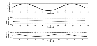
Figure 1: Outputs and input signals in the nominal case (reference trajectory and constraints limits in dashed-line, obtained signals in solid-line)

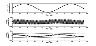
Figure 2: Outputs and input signals in the uncertain case with nominal MPC control (reference trajectory and constraints limits in dashed-line, obtained signals in solid-line)

First, to have a base-line performance, we solve the nominal MPC problem, i.e. without model uncertainties. We report the corresponding results on Figure 1, where it is clear that the desired load angular position is precisely tracked, without violating the shaft torque and the control voltage constraints. Next, we introduce the parametric model uncertainty $\delta\beta_{l}=-70\;[Nms/rad]$. Note that we purposely introduced a very large model uncertainty, i.e. more than $100\%$ of the nominal value, to show clearly the bad effect of this uncertainty on the nominal MPC algorithm and to subsequently test the iterative learning MPC algorithm on a challenging case. We first apply the nominal MPC controller to the uncertain model, we show the obtained performance on Figure 2, where it is clear that the nominal performance is lost, since the second output, i.e. the shaft torque, is oscillating and is violating its upper and lower limits. Furthermore, this oscillations are also present on the control voltage signal.

Now, we apply the iterative learning MPC Algorithm I, where we set $\delta T_{\rm mes}=1.5T_{ref}$. We choose the MES learning cost function as

$$Q = \sum_{i=0}^{N_{E}-1}\|[y_{e}(t-i\delta T_{mpc})]_{1}\|^{2}+\|[\dot{y}_{e}(t-i\delta T_{mpc})]_{1}\|^{2}$$

$$\qquad+\|[y_{e}(t-i\delta T_{mpc})]_{2}\|^{2},$$

i.e. the norm of the error in the load angular position and velocity, plus the norm of the error on the shaft torque. To learn the uncertain parameter $\beta_{l}$, we apply the algorithm (10), as

$$\begin{array}[]{l}{z}_{\beta_{l}}(k^{{}^{\prime}}+1)=z_{\beta_{l}}(k^{{}^{\prime}})+a_{\beta_{l}}\delta T_{mes}sin(\omega_{\beta_{l}}k^{{}^{\prime}}\delta T_{mes}+\frac{\pi}{2})Q\\ \delta\hat{\beta}_{l}(k^{{}^{\prime}}+1)=z_{\beta_{l}}(k^{{}^{\prime}}+1)+a_{\beta_{l}}sin(\omega_{\beta_{l}}k^{{}^{\prime}}\delta T_{mes}-\frac{\pi}{2}),\end{array}$$ (14)

with $a_{\beta_{l}}=10^{-6},\;\omega_{\beta_{l}}=0.7\;rad/s$. We select $\omega_{\beta_{l}}$ to be higher than the desired frequency of the closed-loop (around $0.1\;rad/s$), to ensure convergence of the MES algorithm, since the ES algorithms convergence proofs are based on averaging theory, which assumes high dither frequencies, e.g. [9, 10]. We chose a small value of the dither signal amplitude, since we noticed that the MES cost function has large values due to the large simulated uncertainty, so to keep the search excursion amplitude small, and converge to a precise value of the uncertainty $\delta\beta_{l}$, i.e. to keep $a_{\beta_{l}}Q$ small, we choose small $a_{\beta_{l}}$ (for further explanations on how to tune MES algorithms please refer to [36]). We also set the MES cost function threshold $\epsilon_{Q}$ to $1.5Q_{nominal}$, where $Q_{nominal}$ is the value of the MES cost function obtained in the nominal-model case with the nominal MPC, i.e. the base-line ideal case. In other words, we decide to stop searching for the best estimation of the value of the uncertainty when the uncertain MES cost function, i.e., the value of $Q$ when applying the iterative learning MPC algorithm to the uncertain model, is less or equal to $1.5$ of the MES cost function in the case without model uncertainties, which represents the best achievable MES cost function.

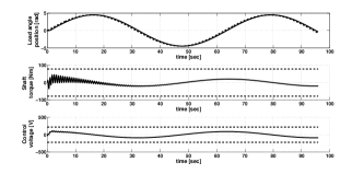
Figure 3: Outputs and input signals in the uncertain case with iterative learning MPC (reference trajectory and constraints limits in dashed-line, obtained signals in solid-line)

Figure 4: MES cost function evolution over the learning iterations

Figure 5: Uncertain parameter learning evolution over the learning iterations

The obtained results of the iterative learning MPC algorithm are reported on Figures 3, 4 and 5. First, note on Figure 4, that the uncertain cost function initial value (at the first iteration of the MES learning) is very high, about $4.5\cdot 10^{6}$, which is about $50$ times the value of the nominal base-line MES cost function value. We see on Figure 4 that this cost function decreases as expected along the MES learning iterations to reach a small value after about $25$ iterations. This corresponds to the required number of iterations to learn the actual value of the uncertain parameter as shown on Figure 5. Eventually, after the convergence of the learning algorithm, we see on Figure 3, that the nominal base-line performances of the MPC are recovered and that the output track the desired reference with smooth signals and without violating the desired constraints.

Figure 6: Outputs and input signals in the uncertain case with nominal MPC control (reference trajectory and constraints limits in dashed-line, obtained signals in solid-line)

We also tested the case of multiple uncertainties. We assumed the two uncertainties $\delta{\beta}_{l}=-70,\;[Nms/rad]$, $\delta{J}_{l}=-0.2,\;[kgm^{2}]$. We first show on Figure 6 the performance of the nominal MPC when applied to this uncertain model. It is clear that the nominal MPC cannot cope with the uncertainties effect on the system’s performance, since the shaft torque, is oscillating and is violating its limits. The control voltage signal experiences oscillations, as well. Next, we apply the iterative learning-based MPC, where $\hat{\delta\beta}_{l}$ is learned using (14), and $\hat{\delta J}_{l}$ is learned using the ES equations

$$\begin{array}[]{l}{z}_{J_{l}}(k^{{}^{\prime}}+1)=z_{J_{l}}(k^{{}^{\prime}})+a_{J_{l}}\delta T_{mes}sin(\omega_{J_{l}}k^{{}^{\prime}}\delta T_{mes}+\frac{\pi}{2})Q\\ \delta\hat{J}_{l}(k^{{}^{\prime}}+1)=z_{J_{l}}(k^{{}^{\prime}}+1)+a_{J_{l}}sin(\omega_{J_{l}}k^{{}^{\prime}}\delta T_{mes}-\frac{\pi}{2}),\end{array}$$ (15)

with $a_{J_{l}}=10^{-8}$, and $\omega_{J_{l}}=0.8\;rad/s$. Note that we choose a smaller dither amplitude for the $\delta J_{l}$ estimation, since the value of the uncertainty on $J_{l}$ is smaller, so we need a smaller dither signal amplitude for the search of the uncertain value.

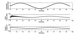
Figure 7: Outputs and input signals in the uncertain case with iterative learning MPC (reference trajectory and constraints limits in dashed-line, obtained signals in solid-line)

Figure 8: MES cost function evolution over the learning iterations

The results of the iterative learning MPC algorithm in this case are reported on Figure s 7, 8, 9 and 10. The learning cost function shown on Figure 8, is clearly decreasing and stabilizes after about $30$ iterations. The uncertainties are learned and the overall tracking performance is recovered, as shown on Figures 9, 10 and 7, respectively. We notice here that the estimation of the uncertainties has some small residual error, this estimation error can be improved by either fine tuning the MES dither signals’ amplitudes, e.g., by using a time-varying dither amplitude [37], or by choosing other type of MES algorithms with larger domain of attraction, e.g. [12, 38].

Figure 9: Uncertain parameter $\delta\beta_{l}$ learning evolution over the learning iterations

Figure 10: Uncertain parameter $\delta J_{l}$ learning evolution over the learning iterations

V Conclusion

In this paper, we have reported some preliminary results about an MES-based adaptive MPC algorithm. We have argued that it is possible to merge together a model-based linear MPC algorithm with a model-free MES algorithm to iteratively learn structural model uncertainties and thus improve the overall performance of the MPC controller. We have discussed a possible direction to analyze the stability of such algorithms. However, a more rigorous analysis of the stability and convergence of the proposed algorithm is under development, and will be presented in our future reports. We have reported encouraging numerical results obtained on a mechatronics example, namely, a DC servo-motor control example. Future investigations will focus on improving the convergence rate of the iterative learning MPC algorithm, by using different ES algorithms with semi-global convergence properties, e.g. [12, 38], and on extending this work to different types of model-free learning algorithms, e.g. reinforcement learning algorithms, and comparing the learning algorithms in terms of their convergence rate and achievable optimal performances.

References

- [1] D. Q. Mayne, J. B. Rawlings, C. V. Rao, and P. O. M. Scokaert, “Constrained model predictive control: Stability and optimality,” Automatica, vol. 36, pp. 789–814, 2000.
- [2] E. Hartley, J. Jerez, A. Suardi, J. Maciejowski, E. Kerrigan, and G. Constantinides, “Predictive control of a boeing 747 aircraft using an fpga,” in Proc. 4th IFAC Nonlinear Model Predictive Control Conference, Noordwijkerhout, The Netherlands, 2012, pp. 80–85.
- [3] S. Di Cairano, H. Park, and I. Kolmanovsky, “Model predictive control approach for guidance of spacecraft rendezvous and proximity maneuvering,” 2012, special Issue dedicated to Prof. David W. Clarke. In press.
- [4] S. Di Cairano, D. Yanakiev, A. Bemporad, I. Kolmanovsky, and D. Hrovat, “Model predictive idle speed control: Design, analysis, and experimental evaluation,” IEEE, Transactions on Control Systems Technology, vol. 20, no. 1, pp. 84 –97, 2012.
- [5] S. Di Cairano, H. Tseng, D. Bernardini, and A. Bemporad, “Vehicle yaw stability control by coordinated active front steering and differential braking in the tire sideslip angles domain,” IEEE, Transactions on Control Systems Technology, pp. 1–13, 2012, in press.
- [6] S. Di Cairano, A. Bemporad, I. Kolmanovsky, and D. Hrovat, “Model predictive control of magnetically actuated mass spring dampers for automotive applications,” Int. Journal of Control, vol. 80, no. 11, pp. 1701–1716, 2007.
- [7] A. Grancharova and T. Johansen, “Explicit model predictive control of an electropneumtaic clutch actuator using on/off valves and pulsewidth modulation,” in European Control Conference, Budapest, Hungary, 2009, pp. 4278–4283.
- [8] K. Ariyur and M. Krstić, Real-time optimization by extremum-seeking control. Wiley-Blackwell, 2003.
- [9] K. B. Ariyur and M. Krstic, “Multivariable extremum seeking feedback: Analysis and design,” in Proc. of the Mathematical Theory of Networks and Systems, South Bend, IN, August 2002.
- [10] D. Nesic, “Extremum seeking control: Convergence analysis,” European Journal of Control, vol. 15, no. 3 4, pp. 331 – 347, 2009.
- [11] M. Krstic, “Performance improvement and limitations in extremum seeking,” Systems Control Letters, vol. 39, pp. 313–326, 2000.
- [12] Y. Tan, D. Nesic, and I. Mareels, “On non-local stability properties of extremum seeking control,” Automatica, no. 42, pp. 889–903, 2006.
- [13] M. Rotea, “Analysis of multivariable extremum seeking algorithms,” in Proceedings of the American Control Conference, vol. 1, no. 6. IEEE, 2000, pp. 433–437.
- [14] M. Guay, S. Dhaliwal, and D. Dochain, “A time-varying extremum-seeking control approach,” in American Control Conference, 2013.
- [15] T. Zhang, M. Guay, and D. Dochain, “Adaptive extremum seeking control of continuous stirred-tank bioreactors,” AIChE J., no. 49, p. 113 123., 2003.
- [16] N. Hudon, M. Guay, M. Perrier, and D. Dochain, “Adaptive extremum-seeking control of convection-reaction distributed reactor with limited actuation,” Computers Chemical Engineering, vol. 32, no. 12, pp. 2994 – 3001, 2008.
- [17] C. Zhang and R. Ord ez, Extremum-Seeking Control and Applications. Springer-Verlag, 2012.
- [18] M. Benosman and G. Atinc, “Multi-parametric extremum seeking-based learning control for electromagnetic actuators,” in American Control Conference, 2013.
- [19] ——, “Nonlinear learning-based adaptive control for electromagnetic actuators,” in European Control Conference, 2013.
- [20] A. Feldbaum, “Dual control theory,” Automation and Remote Control, vol. 21, no. 9, pp. 874–1039, 1960.
- [21] M. S. Lobo and S. Boyd, “Policies for simultaneous estimation and optimization,” in American Control Conference, 1999, pp. 958ñ–964.
- [22] O. A. Sotomayor, D. Odloak, and L. F. Moro, “Closed-loop model re-identification of processes under MPC with zone control,” Control Engineering Practice, vol. 17, no. 5, pp. 551 – 563, 2009.
- [23] H. Jansson and H. Hjalmarsson, “Input design via LMIs admitting frequency-wise model specifications in confidence regions,” IEEE, Transactions on Automatic Control, vol. 50, no. 10, pp. 1534–1549, 2005.
- [24] G. Marafioti, R. R. Bitmead, and M. Hovd, “Persistently exciting model predictive control,” International Journal of Adaptive Control and Signal Processing, 2013.
- [25] E. Žáčeková, S. Prívara, and M. Pčolka, “Persistent excitation condition within the dual control framework,” Journal of Process Control, vol. 23, no. 9, pp. 1270–1280, 2013.
- [26] J. Rathouskỳ and V. Havlena, “MPC-based approximate dual controller by information matrix maximization,” International Journal of Adaptive Control and Signal Processing, vol. 27, no. 11, pp. 974–999, 2013. [Online]. Available: http://dx.doi.org/10.1002/acs.2370
- [27] H. Genceli and M. Nikolaou, “New approach to constrained predictive control with simultaneous model identification,” AIChE Journal, vol. 42, no. 10, pp. 2857–2868, 1996.
- [28] C. A. Larsson, M. Annergren, H. Hjalmarsson, C. R. Rojas, X. Bombois, A. Mesbah, and P. E. Modén, “Model predictive control with integrated experiment design for output error systems,” in American Control Conference, 2013.
- [29] T. A. N. Heirung, B. E. Ydstie, and B. Foss, “An adaptive model predictive dual controller,” in Adaptation and Learning in Control and Signal Processing, vol. 11, no. 1, 2013, pp. 62–67.
- [30] V. Adetola, D. DeHaan, and M. Guay, “Adaptive model predictive control for constrained nonlinear systems,” Systems & Control Letters, vol. 58, no. 5, pp. 320–326, 2009.
- [31] A. González, A. Ferramosca, G. Bustos, J. Marchetti, and D. Odloak, “Model predictive control suitable for closed-loop re-identification,” in American Control Conference. IEEE, 2013, pp. 1709–1714.
- [32] A. Aswani, H. Gonzalez, S. S. Sastry, and C. Tomlin, “Provably safe and robust learning-based model predictive control,” Automatica, vol. 49, no. 5, pp. 1216–1226, 2013.
- [33] M. Benosman, “Learning-based adaptive control for nonlinear systems,” in European Control Conference, 2014, pp. 920–925.
- [34] J. Hadamard, “Sur les probl mes aux d riv es partielles et leur signification physique,” Princeton University Bulletin, pp. 49–52, 1902.
- [35] S. Di Cairano, M. Brand, and S. Bortoff, “Projection-free parallel quadratic programming for linear model predictive control,” Int. Journal of Control, vol. 86, no. 8, pp. 1367–1385, 2013.
- [36] Y. Tan, D. Nesic, and I. Mareels, “On the dither choice in extremum seeking control,” Automatica, no. 44, pp. 1446–1450, 2008.
- [37] W. Moase, C. Manzie, and M. Brear, “Newton-like extremum seeking part I: Theory,” in IEEE, Conference on Decision and Control, December 2009, pp. 3839–3844.
- [38] W. Noase, Y. Tan, D. Nesic, and C. Manzie, “Non-local stability of a multi-variable extremum-seeking scheme,” in IEEE, Australian Control Conference, November 2011, pp. 38–43.