Multi-Parametric Extremum Seeking-based Auto-Tuning for Robust Input-Output Linearization Control

Abstract

We study in this paper the problem of iterative feedback gains tuning for a class of nonlinear systems. We consider Input-Output linearizable nonlinear systems with additive uncertainties. We first design a nominal Input-Output linearization-based controller that ensures global uniform boundedness of the output tracking error dynamics. Then, we complement the robust controller with a model-free multi-parametric extremum seeking (MES) control to iteratively auto-tune the feedback gains. We analyze the stability of the whole controller, i.e. robust nonlinear controller plus model-free learning algorithm. We use numerical tests to demonstrate the performance of this method on a mechatronics example.

I Introduction

Input-Output feedback linearization with static state feedback is a very well known nonlinear control approach, which has been extensively used to solve trajectory tracking for nonlinear systems [1]. Its robust version has also been extensively studied, e.g. [2, 3, 4, 5]. The main approaches proposed, either combine a linear robust controller with the linearization controller to achieve some robustness w.r.t. to structural model uncertainties and measurable disturbances, e.g. [4] and references therein, or use high gains observers to estimate the input disturbance and use the estimation to compensate for the disturbance and recover some performance of the feedback linearization controller, e.g.[2]. In this work we focus on specific problem for Input-Output feedback linearization control, namely, iterative feedback gains tuning.
Indeed, the use of learning algorithm to tune feedback gains of nominal linear controllers to achieve some desired performances has been studied in several papers, e.g. [6, 7, 8, 9]. In this work, we try to extend these approaches to a more general setting of uncertain nonlinear systems (refer to [10] for preliminary results). We consider here a particular class of nonlinear systems, namely, nonlinear models affine in the control input, which are linearizable via static state feedback. We consider bounded additive model uncertainties with known upper bound function. We propose a simple modular iterative gains tuning controller, in the sense that we first design a passive robust controller, based on the classical Input-Output linearization method merged with a Lyapunov reconstruction-based control, e.g. [11, 12]. This passive robust controller ensures uniform boundedness of the tracking errors and their convergence to a given invariant set. Next, in a second phase we add a multi-variable extremum seeking algorithm to iteratively auto-tune the feedback gains of the passive robust controller to optimize a desired system performance, which is formulated in terms of a desired cost function minimization.
This paper is organized as follows: First, some notations and definitions are recalled in Section II. Next, we present the class of systems studied here and formulate the control problem in Section III. The proposed control approach together with the closed-loop dynamic solutions boundedness are presented in Section IV. Section V is dedicated to the application of the controller to a mechatronics example. Finally the paper ends with a summarizing conclusion in Section VI.

II Notations and definitions

Throughout the paper we will use $|.|$ to denote the Euclidean norm; i.e., for $x\in\mathbb{R}^{n}$ we have $|x|=\sqrt{x^{T}x}$. We will use the notations $diag\{m_{1},...,m_{n}\}$ for $n\times n$ diagonal matrix, $z(i)$ denotes the $i$th element of the vector $z$. We use $\dot{(.)}$ for the short notation of time derivative and $f^{(r)}(t)$ for $\frac{d^{r}f(t)}{dt^{r}}$. $Max(V)$ denotes the maximum element of a vector $V$, and $sgn(.)$ denotes for the sign function. We denote by $\mathbb{C}^{k}$ functions that are $k$ times differentiable, and by $\mathbb{C}^{\infty}$ a smooth function. A function is said analytic in a given set, if it admits a convergent Taylor series approximation in some neighborhood of every point of the set. An impulsive dynamical system is said to be well-posed if it has well defined distinct resetting times, admits a unique solution over a finite forward time interval and does not exhibits any Zeno solutions, i.e. an infinitely many resetting of the system in finite time interval [13]. Finally, in the sequel when we talk about error trajectories boundedness, we mean uniform boundedness as defined in [11] (p.167, Definition 4.6 ) for nonlinear continuous systems, and in [13] (p. 67, Definition 2.12) for time-dependent impulsive dynamical systems.

III Problem formulation

III-A Class of systems

We consider here affine uncertain nonlinear systems of the form:

$$\begin{array}[]{c}\dot{x}=f(x)+\Delta f(x)+g(x)u,\;x(0)=x_{0}\\ y=h(x),\end{array}$$ (1)

where $x\in\mathbb{R}^{n},u\in\mathbb{R}^{n_{a}},y\in\mathbb{R}^{m}\;(n_{a}\geq m)$, represent respectively the state, the input and the controlled output vectors, $x_{0}$ is a known initial condition, $\Delta f(x)$ is a vector field representing additive model uncertainties. The vector fields $f$, $\Delta f$, columns of $g$ and function $h$ satisfy the following assumptions.

Assumption 1

$f:\mathbb{R}^{n}\rightarrow\mathbb{R}^{n}$ and the columns of $g:\mathbb{R}^{n}\rightarrow\mathbb{R}^{n\times n_{a}}$ are $\mathbb{C}^{\infty}$ vector fields on a bounded set $X$ of $\mathbb{R}^{n}$ and $h(x)$ is a $\mathbb{C}^{\infty}$ function on $X$. The vector field $\Delta f(x)$ is $\mathbb{C}^{1}$ on $X$.

Assumption 2

System (1) has a well-defined (vector) relative degree $\{r1,\dots,rm\}$ at each point $x^{0}\in X$, and the system is linearizable, i.e. $\sum_{i=1}^{i=m}r{i}=n$ (see e.g. [1]).

Assumption 3

The uncertainty vector $\Delta f$ is s.t. $|\Delta f(x)|\leq d(x)\;\forall x\in X$, where $d\;:\;X\rightarrow\mathbb{R}$ is a smooth nonnegative function.

Assumption 4

The desired output trajectories $y_{id}$ are smooth functions of time, relating desired initial points $y_{i0}$ at $t=0$ to desired final points $y_{if}$ at $t=t_{f}$, and s.t. $y_{id}(t)=y_{if},\;\forall t\geq t_{f},\;t_{f}>0$, $i\in\{1,...,m\}$.

III-B Control objectives

Our objective is to design a feedback controller $u(x,K)$, which ensures for the uncertain model (1) uniform boundedness of a tracking error, and for which the stabilizing feedback gains vector $K$ is iteratively auto-tuned, to optimize a desired performance cost function.
We stress here that the goal of the gain auto-tuning is not stabilization but rather performance optimization. To achieve this control objective, we proceed as follows: We design a ‘passive’ robust controller which ensures boundedness of the tracking error dynamics, and we combine it with a model-free learning algorithm to iteratively (resting from the same initial condition at each iteration) auto-tune the feedback gains of the controller, and optimize online a desired performance cost function.

IV Controller design

IV-A Step one: Passive robust control design

Under Assumption 2 and nominal conditions, i.e. $\Delta f=0$, system (1) can be written as [1]:

$$\begin{array}[]{l}y^{(r)}(t)=b(\xi(t))+A(\xi(t))u(t),\\ \end{array}$$ (2)

where

$$\begin{array}[]{l}y^{(r)}(t)\triangleq(y_{1}^{(r_{1})}(t),\dots,y_{m}^{(r_{m})}(t))^{T},\\ \xi(t)=(\xi^{1}(t),\dots,\xi^{m}(t))^{T},\\ \xi^{i}(t)=(y_{i}(t),\dots,y_{i}^{(ri-1)}(t)),\;\;1\leq i\leq m,\end{array}$$ (3)

and $b,A$ write as functions of $f,g,h$, and $A$ is non-singular in $X$ ([1], pp. 234-288).
At this point we introduce one more assumption on the system.

Assumption 5

We assume that the additive uncertainties $\Delta f$ in (1) appear as additive uncertainties in the linearized model (2), (3), as follows

$$\begin{array}[]{l}y^{(r)}=b(\xi)+\Delta b(\xi)+A(\xi)u,\\ \end{array}$$ (4)

where $\Delta b$ is $\mathbb{C}^{1}$ on $\tilde{X}$, and s.t. $|\Delta b(\xi)|\leq d_{2}(\xi)\;\forall\xi\in\tilde{X}$, where $d_{2}\;:\;\tilde{X}\rightarrow\mathbb{R}$ is a smooth nonnegative function, and $\tilde{X}$ is the image of the set $X$ by the diffeomorphism $x\rightarrow\xi$ between the states of (1) and (2).

Remark 1

Assumption 5, can be ensured under the so-called matching conditions ([14], p. 146).

If we consider the nominal model (2) first, we can define a virtual input vector $v$ as

$$b(\xi(t))+A(\xi(t))u(t)=v(t).$$ (5)

Combining (2) and (5), we obtain the linear (virtual) Input-Output mapping

$$y^{(r)}(t)=v(t).$$ (6)

Based on the linear system (6), we propose the stabilizing output feedback for the nominal system (4) with $\Delta b(\xi)=0$, as

$$\begin{array}[]{l}u_{nom}=A^{-1}(\xi)(v_{s}(t,\xi)-b(\xi)),\;v_{s}=(v_{s1},...,v_{sm})^{T}\\ v_{si}={y_{i}}^{(ri)}_{d}-K^{i}_{ri}({y_{i}}^{(ri-1)}-{y_{i}}^{(ri-1)}_{d})-...-K^{i}_{1}(y_{i}-{y_{i}}_{d}),\\ i\in\{1,...,m\}.\end{array}$$ (7)

Denoting the tracking error vector as $e_{i}(t)=y_{i}(t)-{y_{i}}_{d}(t)$, we obtain the tracking error dynamics

$$e_{i}^{(r_{i})}(t)+K^{i}_{r_{i}}e_{i}^{(r_{i}-1)}(t)+...+K^{i}_{1}e_{i}(t)=0,\;i=1,...,m,$$ (8)

and by tuning the gains $K^{i}_{j},\;i=1,...,m,\;j=1,...,r_{i}$ such that all the polynomials in (8) are Hurwitz, we obtain global asymptotic stability of the tracking errors $e_{i}(t),\;i=1,...m$, to zero. To formalize this condition let us state the following assumption.

Assumption 6

We assume that there exist a nonempty set $\mathcal{K}$ of gains $K^{i}_{j},\;i=1,...,m,\;j=1,...,r_{i}$, such that the polynomials (8) are Hurwitz.

Remark 2

Assumption 6 is well know in the Input-Output linearization control literature. It simply states that we can find gains that stabilize the polynomials (8), which can be done for example by pole placements.

Next, if we consider that $\Delta b(\xi)\neq 0$ in (4), the global asymptotic stability of the error dynamics will not be guarantied anymore due to the additive error vector $\Delta b(\xi)$, we then choose to use Lyapunov reconstruction technique (e.g. [12]) to obtain a controller ensuring practical stability of the tracking error. This controller is presented in the following Theorem.

Theorem 1

Consider the system (1) for any $x_{0}\in\mathbb{R}^{n}$, under Assumptions 1, 2, 3, 4, 5 and 6, with the feedback controller

$$\begin{array}[]{l}u=A^{-1}(\xi)(v_{s}(t,\xi)-b(\xi))-A^{-1}(\xi)(\frac{\partial V}{\partial z}_{ind})^{{}^{\prime}}k\;d_{2}(e),\\ k>0,\;\;v_{s}=(v_{s1},...,v_{sm})^{T}\\ v_{si}={y_{i}}^{(ri)}_{d}-K^{i}_{ri}({y_{i}}^{(ri-1)}-{y_{i}}^{(ri-1)}_{d})-...-K^{i}_{1}(y_{i}-{y_{i}}_{d}).\end{array}$$ (9)

Where, $K^{i}_{j}\in\mathcal{K},\;j=1,...,ri,\;i=1,...,m$, and $\frac{\partial V}{\partial z}_{ind}=(\frac{\partial V}{\partial z(r1)},...,\frac{\partial V}{\partial z(rm)}),\;V=z^{T}Pz$, $P>0$ such that $P\tilde{A}+\tilde{A}^{T}P=-I$, with $\tilde{A}$ being an $n\times n$ matrix defined as

$$\tilde{A}=\left(\begin{array}[]{l}0,1,0,...................................,0\\ 0,0,1,0,................................,0\\ \hskip 56.9055pt\ddots\\ -K^{1}_{1},...,-K^{1}_{r1},0,..................,0\\ \hskip 56.9055pt\ddots\\ 0,...................,0,1,0,...........,0\\ 0,...................,0,0,1,...........,0\\ \hskip 56.9055pt\ddots\\ 0,................,0,-K^{m}_{1},...,-K^{m}_{rm}\end{array}\right),$$ (10)

and $z=(z^{1},...,z^{m})^{T},\;z^{i}=(e_{i},...,e_{i}^{r_{i}-1}),\;i=1,...,m$. Then, the vector $z$ is uniformly bounded and reached the positive invariant set $S=\{z\in\mathbb{R}^{n}|\;1-k\;|\frac{\partial V}{\partial z}_{ind}|\geq 0\}$.

Proof: The proof has been removed due to space constraints. It will appear in a longer journal version of this work.

IV-B Iterative tuning of the feedback gains

In Theorem 1, we showed that the passive robust controller (9) leads to bounded tracking errors attracted to the invariant set $S$ for a given choice of the feedback gains $K^{i}_{j},\;j=1,...,ri,\;i=1,...,m$. Next, to iteratively tune the feedback gains of (9), we define a desired cost function, and use a multi-variable extremum seeking to iteratively auto-tune the gains and minimize the defined cost function. We first denote the cost function to be minimized as $Q(z(\beta))$ where $\beta$ represents the optimization variables vector, defined as

$$\beta=[\delta K^{1}_{1},...,\delta K^{1}_{r1},...,\delta K^{m}_{1},...,\delta K^{m}_{rm},\delta k]^{T}$$ (11)

such that the updated feedback gains write as

$$\begin{array}[]{c}K^{i}_{j}=K^{i}_{j-nominal}+\delta K^{i}_{j},\;j=1,...ri,\;i=1,...,m.\\ k=k_{nominal}+\delta k,\;\;k_{nominal}>0\end{array}$$ (12)

where $K^{i}_{j-nominal},\;j=1,...ri,\;i=1,...,m$ are the nominal initial values of the feedback gains chosen such that Assumption (5) is satisfied.

Remark 3

The choice of the cost function $Q$ is not unique. For instance, if the controller tracking performance at the time specific instants $It_{f},\;I=1,2,3...$ is important for the targeted application (see the example presented in Section V), one can choose $Q$ as

$$Q(z(\beta))=z^{T}(It_{f})C_{1}z(It_{f}),\;\;C_{1}>0$$ (13)

If other performance needs to be optimized over a finite time interval, for instance a combination of a tracking performance and a control power performance, then one can choose for example the cost function

$$\begin{array}[]{l}Q(z(\beta))=\int_{(I-1)t_{f}}^{It_{f}}z^{T}(t)C_{1}z(t)dt+\int_{(I-1)t_{f}}^{It_{f}}u^{T}(t)C_{2}u(t)dt,\\ I=1,2,3...,\;C_{1},\;C_{2}>0\end{array}$$ (14)

The gains variation vector $\beta$ is then used to minimize the cost function $Q$ over the iterations $I\in\{1,2,3,...\}$.

Following multi-parametric extremum seeking theory [15], the variations of the gains are defined as

$$\begin{array}[]{l}\dot{x}_{K^{i}_{j}}=a_{K^{i}_{j}}sin(\omega_{K^{i}_{j}}t-\frac{\pi}{2})Q(z(\beta))\\ \delta{\hat{K}}^{i}_{j}(t)=x_{K^{i}_{j}}(t)+a_{K^{i}_{j}}sin(\omega_{K^{i}_{j}}t+\frac{\pi}{2}),\;j=1,...ri,\;i=1,...,m\\ \dot{x}_{k}=a_{k}sin(\omega_{k}t-\frac{\pi}{2})Q(z(\beta))\\ \delta\hat{k}(t)=x_{k}(t)+a_{k}sin(\omega_{k}t+\frac{\pi}{2}),\\ \end{array}$$ (15)

where $a_{K^{i}_{j}},\;j=1,...ri,\;i=1,...,m,\;a_{k}$ are positive tuning parameters, and

$$\begin{array}[]{l}\omega_{1}+\omega_{2}\neq\omega_{3},\;\text{for}\;\omega_{1}\neq\omega_{2}\neq\omega_{3},\\ \forall\omega_{1},\omega_{2},\omega_{3}\in\{\omega_{K^{i}_{j}},\omega_{k},\;j=1,...ri,\;i=1,...,m\},\end{array}$$ (16)

with $\omega_{i}>\omega^{*},\;\forall\omega_{i}\in\{\omega_{K^{i}_{j}},\omega_{k},\;j=1,...ri,\;i=1,...,m\}$, $\omega^{*}$ large enough.
To study the stability of the learning-based controller, i.e. controller (9), with the varying gains (12) and (15), we first need to introduce some additional Assumptions.

Assumption 7

We assume that the cost function $Q$ has a local minimum at $\beta^{*}$.

Assumption 8

We consider that the initial gain vector $\beta$ is sufficiently close to the optimal gain vector $\beta^{*}$.

Assumption 9

The cost function is analytic and its variation with respect to the gains is bounded in the neighborhood of $\beta^{*}$, i.e. $|\frac{\partial{Q}}{\partial\beta}({\tilde{\beta}})|\leq\Theta_{2},\;\Theta_{2}>0,\;\tilde{\beta}\in\mathcal{V}(\beta^{*})$, where $\mathcal{V}(\beta^{*})$ denotes a compact neighborhood of $\beta^{*}$.

We can now state the following result.

Theorem 2

Consider the system (1) for any $x_{0}\in\mathbb{R}^{n}$, under Assumptions 1, 2, 3, 4, 5 and 6, with the feedback controller

$$\begin{array}[]{l}u=A^{-1}(\xi)(v_{s}(t,\xi)-b(\xi))-A^{-1}(\xi)(\frac{\partial V}{\partial z}_{ind})^{{}^{\prime}}k(t)\;d_{2}(e),\\ k>0,\;\;v_{s}=(v_{s1},...,v_{sm})^{T},\\ v_{si}(t,\xi)=\hat{{y}_{i}}^{(ri)}_{d}-K^{i}_{ri}(t)({y_{i}}^{(ri-1)}-\hat{y_{i}}^{(ri-1)}_{d})-...\\ -K^{i}_{1}(t)({y_{i}}-\hat{y_{i}}_{d}),\;i=1,...,m\end{array}$$ (17)

Where, the state vector is reset following the resetting law $x(It_{f})=x_{0},\;I\in\{1,2,...\}$, the desired trajectory vector is rest following $\hat{y_{i}}_{d}(t)=y_{id}(t-(I-1)t_{f}),\;(I-1)t_{f}\leq t<It_{f},\;I\in\{1,2,...\}$, and $K^{i}_{j}(t)\in\mathcal{K},\;j=1,...,ri,\;i=1,...,m$ are piecewise continues gains switched at each iteration $I$, $I\in\{1,2,...\}$, following the update law

$$\begin{array}[]{l}K^{i}_{j}(t)=K^{i}_{j-nominal}+\delta K^{i}_{j}(t)\\ \delta K^{i}_{j}(t)=\delta{\hat{K}}^{i}_{j}((I-1)t_{f}),\;(I-1)t_{f}\leq t<It_{f},\\ k(t)=k_{nominal}+\delta k(t),\;\;k_{nominal}>0\\ \delta k(t)=\delta\hat{k}((I-1)t_{f}),\;(I-1)t_{f}\leq t<It_{f},\;I=1,2,3...\\ \end{array}$$ (18)

where $\delta{\hat{K}}^{i}_{j},\delta\hat{k}$ are given by (15), (16) and whereas the rest of the coefficients are defined similarly to Theorem 1. Then, the obtained closed-loop impulsive time-dependent dynamic system (1), (15), (16), (17) and (18), is well posed, the tracking error $z$ is uniformly bounded, and is steered at each iteration $I$ towards the positive invariant set $S_{I}=\{z\in\mathbb{R}^{n}|\;1-k_{I}\;|\frac{\partial V}{\partial z}_{ind}|\geq 0\}$, $k_{I}=\beta_{I}(n+1)$, where $\beta_{I}$ is the value of $\beta$ at the $I$th iteration. Furthermore, $|Q(\beta(It_{f}))-Q(\beta^{*})|\leq\Theta_{2}\big{(}\frac{\Theta_{1}}{\omega_{0}}+\sqrt{\sum\limits_{\small i=1,...,m\;j=1,...,ri}{a_{K^{i}_{j}}}^{2}+{a_{k}}^{2}}\big{)},\;\Theta_{1},\;\Theta_{2}>0,\;\text{for }\;I\rightarrow\infty$, where $\omega_{0}=Max(\omega_{K^{1}_{1}},...,\omega_{K^{m}_{rm}},\omega_{k})$, and $Q$ satisfies Assumptions 7, 8 and 9. Wherein, the vector $\beta$ remains bounded over the iterations s.t. $|\beta((I+1)t_{f})-\beta(It_{f})|\leq 0.5t_{f}Max({a_{K^{1}_{1}}}^{2},...,{a_{K^{m}_{rm}}}^{2},a_{k}^{2})\Theta_{2}+t_{f}\omega_{0}\sqrt{\sum\limits_{\small i=1,...,m\;j=1,...,ri}{a_{K^{i}_{j}}}^{2}+{a_{k}}^{2}},\;I\in\{1,2,...\}$, and satisfies asymptotically the bound $|\beta(It_{f})-\beta^{*}|\leq\frac{\Theta_{1}}{\omega_{0}}+\sqrt{\sum\limits_{\small i=1,...,m\;j=1,...,ri}{a_{K^{i}_{j}}}^{2}+{a_{k}}^{2}},\;\Theta_{1}>0,\;\text{for}\;I\rightarrow\infty$.

Proof: The proof has been removed due to space constraints. It will appear in a longer journal version of this work.

Remark 4

In Theorem 2, we show that in each iteration $I$, the tracking error vector $z$ is directed toward the invariant set $S_{I}$. However, due to the finite time-interval length $t_{f}$ of each iteration, we cannot guaranty that the vector $z$ enters $S_{I}$ in each iteration (unless we are in the trivial case where $z_{0}\in S_{I}$). All what we guaranty is that the vector norm $|z|$ starts from a bounded value $|z_{0}|$ and remains bounded during the iterations with an upper-bound which can be estimated as function of $|z_{0}|$ by using the bounds of the quadratic Lyapunov functions $V_{I},\;I=1,2,...$, i.e. a uniform boundedness result ([13], p 6, def. 2.12).

In the next section we propose to illustrate this approach on a mechatronics system.

V The case of electromagnetic actuators

We apply here the method presented above to the case of electromagnetic actuators.
System modelling: Following [16, 17], we consider the following nonlinear model for electromagnetic actuators

$$\begin{array}[]{l}m\frac{d^{2}x_{a}}{dt^{2}}=k(x_{0}-x_{a})-\eta\frac{dx_{a}}{dt}-\frac{ai^{2}}{2(b+x_{a})^{2}}\\ u=Ri+\frac{a}{b+x_{a}}\frac{di}{dt}-\frac{ai}{(b+x_{a})^{2}}\frac{dx_{a}}{dt},\;0\leq x_{a}\leq x_{f},\end{array}$$ (19)

where, $x_{a}$ represents the armature position physically constrained between the initial position of the armature $0$, and the maximal position of the armature $x_{f}$, $\frac{dx_{a}}{dt}$ represents the armature velocity, $m$ is the armature mass, $k$ the spring constant, $x_{0}$ the initial spring length, $\eta$ the damping coefficient (assumed to be constant), $\frac{ai^{2}}{2(b+x_{a})^{2}}$ represents the electromagnetic force (EMF) generated by the coil, $a,b$ are two constant parameters of the coil, $R$ the resistance of the coil, $L=\frac{a}{b+x_{a}}$ the coil inductance, $\frac{ai}{(b+x_{a})^{2}}\frac{dx_{a}}{dt}$ represents the back EMF. Finally, $i$ denotes the coil current, $\frac{di}{dt}$ its time derivative and $u$ represents the control voltage applied to the coil. In this model we do not consider the saturation region of the flux linkage in the magnetic field generated by the coil, since we assume a current and armature motion ranges within the linear region of the flux.
Passive robust controller: In this section we first design a nonlinear passive robust control based on Theorem 1.
Follwoing Assumption 4, we define $x_{ref}$ a desired armature position trajectory, s.t. $x_{ref}$ is a smooth (at least $C^{2}$) function satisfying the initial/final constraints: $x_{ref}(0)=0,\;x_{ref}(t_{f})=x_{f},\;\dot{x}_{ref}(0)=0,\;\dot{x}_{ref}(t_{f})=0$, where $t_{f}$ is a desired finite motion time and $x_{f}$ is a desired final position. We consider the dynamical system (19) with bounded parametric uncertainties on the spring coefficient $\delta k$, with $|\delta k|\leq\delta k_{max}$, and the damping coefficient $\delta\eta$, with $|\delta\eta|\leq\delta\eta_{max}$, such that $k=k_{nominal}+\delta k$, $\eta=\eta_{nominal}+\delta\eta$, where $k_{nominal},\;\eta_{nominal}$ are the nominal values of the spring stiffness and the damping coefficient, respectively. If we consider the state vector $x=(x_{a},\;\dot{x}_{a},\;i)^{{}^{\prime}}$, and the controlled output $x_{a}$, the uncertain model of electromagnetic actuators can be written in the form of (1), as

$$\begin{array}[]{l}\dot{x}=\left(\begin{array}[]{l}\dot{x}_{a}\\ \ddot{x}_{a}\\ \dot{i}\end{array}\right)=\left(\begin{array}[]{c}x_{2}\\ \frac{k_{nominal}}{m}(x_{0}-x_{1})-\frac{\eta_{nominal}}{m}x_{2}+...\\ \hskip 85.35826pt...-\frac{ax_{3}^{2}}{2(b+x_{1})^{2}}\\ -\frac{R(b+x_{1})}{a}x_{3}+\frac{x_{3}x_{2}}{b+x_{1}}\end{array}\right)\\ +\left(\begin{array}[]{c}0\\ \frac{\delta k}{m}(x_{0}-x_{1})+\frac{\delta\eta}{m}x_{2}\\ 0\end{array}\right)+\left(\begin{array}[]{c}0\\ 0\\ \frac{b+x_{1}}{a}\end{array}\right)u\\ y=x_{1}.\end{array}$$ (20)

Assumption 1 is clearly satisfied over a nonempty bounded set $X$, as for Assumption 2, it is straightforward to check that if we compute the third time-derivative of the output $x_{a}$, the control variable $u$ appears in a nonsingular expression, which implies that $r=n=3$. Assumption 3 is also satisfied since $|\Delta f(x)|\leq\frac{\delta k_{max}}{m}|x_{0}-x_{1}|+\frac{\delta\eta_{max}}{m}|x_{2}|$.
Next, following the Input-Output linearization method, we can write

$$\begin{array}[]{l}y^{(3)}=x_{a}^{(3)}=-\frac{k_{nominal}}{m}\dot{x}_{a}-\frac{\eta_{nominal}}{m}\ddot{x}_{a}+\frac{Ri^{2}}{(b+x_{a})m}-\\ \frac{\delta k}{m}\dot{x}_{a}-\frac{\delta\eta}{m}\ddot{x}_{a}-\frac{i}{m(b+x_{a})}u,\end{array}$$ (21)

which is of the form of equation (4), with $A=-\frac{i}{m(b+x_{a})},\;b=-\frac{k_{nominal}}{m}\dot{x}_{a}-\frac{\eta_{nominal}}{m}\ddot{x}_{a}+\frac{Ri^{2}}{(b+x_{a})m}$, and the additive uncertainty term $\Delta b=-\frac{\delta k}{m}\dot{x}_{a}-\frac{\delta\eta}{m}\ddot{x}_{a}$, such that $|\Delta b|\leq\frac{\delta k_{max}}{m}|\dot{x}_{a}|+\frac{\delta\eta_{max}}{m}|\ddot{x}_{a}|=d_{2}(x_{a},\dot{x}_{a})$. Let us define the tracking error vector $\mathbf{z}:=(z_{1},\;z_{2},\;z_{3})^{\prime}=(x_{a}-x_{ref},\;\dot{x}_{a}-\dot{x}_{ref},\;\ddot{x}_{a}-\ddot{x}_{ref})^{\prime}$, where $\dot{x}_{ref}=\frac{dx_{ref}(t)}{dt}$, and $\ddot{x}_{ref}=\frac{d^{2}x_{ref}(t)}{dt^{2}}$. Next, using Theorem 1, we can write the following robust passive controller

$$\begin{array}[]{l}u=-\frac{m(b+x_{a})}{i}(v_{s}+\frac{k_{nominal}}{m}\dot{x}_{a}+\frac{\eta_{nominal}}{m}\ddot{x}_{a}-\frac{Ri^{2}}{(b+x_{a})m})+\\ \frac{m(b+x_{a})}{i}\frac{\partial V}{\partial z_{3}}k(\frac{\delta k_{max}}{m}|\dot{x}_{a}|+\frac{\delta\eta_{max}}{m}|\ddot{x}_{a}|),\;k>0\\ v_{s}=x_{ref}^{(3)}(t)+K_{3}(x_{a}^{(2)}-x_{ref}^{(2)}(t))+K_{2}(x_{a}^{(1)}-x_{ref}^{(1)}(t))\\ +K_{1}(x_{a}-x_{ref}(t)),\;K_{i}<0,i=1,2,3.\end{array}$$ (22)

Where, $V=z^{T}Pz$, $P>0$ solution of the equation $P\tilde{\tilde{A}}+\tilde{\tilde{A}}^{T}P=-I$, with

$$\tilde{\tilde{A}}=\left(\begin{array}[]{ccc}0&1&0\\ 0&0&1\\ K_{1}&K_{2}&K_{3}\end{array}\right),$$ (23)

where $K_{1},\;K_{2},\;K_{3}$ are chosen such that $\tilde{\tilde{A}}$ is Hurwitz.
Learning-based auto-tuning of the controller gains: We use now the results of Theorem 2, to iteratively auto-tune the feedback gains of the controller (22). Considering a cyclic behavior of the actuator with each iteration happening over a time interval of length $t_{f}$, following (13) we define the cost function as

$$Q(z(\beta))=C_{1}z_{1}(It_{f})^{2}+C_{2}z_{2}(It_{f})^{2}+C_{3}z_{3}(It_{f})^{2},$$ (24)

where $I=1,2,3...$ is the number of iterations, $C_{1},\;C_{2}>0,\;C_{3}>0$, and $\beta=(\delta K_{1},\;\delta K_{2},\;\delta K_{3},\;\delta k)^{\prime}$, such as the feedback gains write as

$$\begin{array}[]{l}K_{1}=K_{1_{nominal}}+\delta K_{1}\\ K_{2}=K_{2_{nominal}}+\delta K_{2}\\ K_{3}=K_{3_{nominal}}+\delta K_{3}\\ k={k}_{nominal}+\delta{k},\end{array}$$ (25)

where $K_{1_{nominal}},\;K_{2_{nominal}},\;K_{3_{nominal}},\;{k}_{nominal}$ are the nominal initial values of the feedback gains in (22).
Folowing (15), (16), and (18) the variations of the estimated gains are given by

$$\begin{array}[]{l}\dot{x}_{K_{1}}=a_{K_{1}}sin(\omega_{1}t-\frac{\pi}{2})Q(z(\beta))\\ \delta\hat{K}_{1}(t)=x_{K_{1}}(t)+a_{{K}_{1}}sin(\omega_{1}t+\frac{\pi}{2})\\ \dot{x}_{K_{2}}=a_{K_{2}}sin(\omega_{2}t-\frac{\pi}{2})Q(z(\beta))\\ \delta\hat{K}_{2}(t)=x_{{K}_{2}}(t)+a_{{K}_{2}}sin(\omega_{2}t+\frac{\pi}{2})\\ \dot{x}_{{K}_{3}}=a_{K_{3}}sin(\omega_{3}t-\frac{\pi}{2})Q(z(\beta))\\ \delta\hat{K}_{3}(t)=x_{{K}_{3}}(t)+a_{{K}_{3}}sin(\omega_{3}t+\frac{\pi}{2})\\ \dot{x}_{k}=a_{k}sin(\omega_{4}t-\frac{\pi}{2})Q(z(\beta))\\ \delta\hat{k}(t)=x_{k}(t)+a_{k}sin(\omega_{4}t+\frac{\pi}{2})\\ \delta K_{j}(t)=\delta\hat{K}_{j}((I-1)t_{f}),\;(I-1)t_{f}\leq t<It_{f},\\ j\in\{1,2,3\},\;I=1,2,3...\\ \delta k(t)=\delta\hat{k}((I-1)t_{f}),\;(I-1)t_{f}\leq t<It_{f},\;I=1,2,3...\end{array}$$ (26)

where $a_{K_{1}},\;a_{{K}_{2}},\;a_{{K}_{3}},\;a_{k}$ are positive and $\omega_{p}+\omega_{q}\neq\omega_{r},\;p,q,r\in\{1,2,3,4\},\;\text{for}\;p\neq q\neq r.\\$
Simulation results: We show here the behavior of the proposed approach on the electromagnetic actuator example presented in [18], where the model (19) is used with the numerical values of Table I.

Parameter	Value
$m$	$0.27\;[kg]$
$R$	$6\;[\Omega]$
$\eta$	$7.53\;[kg/sec]$
$x_{0}$	$8\;[mm]$
$k$	$158\;[N/mm]$
$a$	$14.96\times 10^{-6}\;[Nm^{2}/A^{2}]$
$b$	$4\times 10^{-5}\;[m]$

TABLE I: Numerical values of the mechanical parameters

The desired trajectory has been selected as the $5th$ order polynomial $x_{ref}(t)=\sum_{i=0}^{5}a_{i}(t/t_{f})^{i}$, where the $a_{i}$’s have been computed to satisfy the boundary constraints $x_{ref}(0)=0,x_{ref}(t_{f})=x_{f},\dot{x}_{ref}(0)=\dot{x}_{ref}(t_{f})=0,\ddot{x}_{ref}(0)=\ddot{x}_{ref}(t_{f})=0$, with $t_{f}=1\;sec$, $x_{f}=0.5\;mm$.
Furthermore, to make the simulation case more challenging we assume an initial error both on the position and the velocity $z_{1}(0)=0.01\;mm$, $z_{2}(0)=0.1\;mm/sec$. Note that these values may seem small, but for this type of actuators it is usually the case that the armature starts form a predefined static position constrained mechanically, so we know that the initial velocity is zero and we know in advance very precisely the initial position of the armature. However, we want to show the performances of the controller on some challenging cases. We also select the nominal feedback gains $K_{1}=-500,\;K_{2}=-125,\;K_{3}=-26,\;k=1$, satisfying Assumption 5. In this test we compare the performances of the passive robust controller (22) with the fixed nominal gains, to the learning controller (22),(25), (26), which was implemented with the cost function (24), where $C_{1}=500,\;C_{2}=500,\;C_{3}=10$, and the learning coefficients for each feedback gain are $\omega_{1}=7.5\;rad/sec$, $\omega_{2}=5.3\;rad/sec$, $\omega_{3}=5.1\;rad/sec$, $\omega_{4}=6.1\;rad/sec$. We point out here that to accelerate the learning convergence rate, which is related to the choice of the coefficients $a_{K_{i}},\;i=1,2,3,\;a_{k}$ , e.g. [19], we have chosen to use a varying amplitude for the coefficients. Indeed, it is well know , e.g. [20], that choosing varying coefficients, which start with a high value to accelerate the search initially and then are tuned down when the cost function becomes smaller, accelerates the learning and achieves a convergence to a tighter neighborhood of the local optimum (due to decrease of the dither amplitudes). To implement this idea, we simply use piece-wise constant coefficients as follows: $a_{{K}_{1}}=200$, $a_{{K}_{2}}=120$, $a_{{K}_{3}}=20$, $a_{{k}}=0.2$, initially and then tuned them down to $a_{{K}_{1}}=200Q(1)/2$, $a_{{K}_{2}}=120Q(1)/2$, $a_{{K}_{3}}=20Q(1)/2$, $a_{{k}}=0.2Q(1)/2$, when $Q\leq Q(1)/2$ and then to $a_{{K}_{1}}=200Q(1)/3$, $a_{{K}_{2}}=120Q(1)/3$, $a_{{K}_{3}}=2Q(1)/3$, $a_{{k}}=0.2Q(1)/3$, when $Q\leq Q(1)/3$, where $Q(1)$ denotes the value of the cost function at the first iteration. We show on figures 1(a), 1(b) the performance of the position and the velocity tracking, with and without the learning algorithm. We see clearly the effect of the learning algorithm that makes the landing velocity closer to the desired zero landing velocity as shown on figure 3(a). The associated coil current and voltage signals are also reposted on figures 2(a) and 2(b), respectively. It is worth mentioning here that the optimized performance in this example is focused mainly on the impact point, i.e. the position and velocity of the armature at $t=t_{f}$, this is why we choose a cost function as (24) instead of a cost function based on the integral of the tracking error. We also report on figure 3(b), the cost function value along the learning iterations. We see a clear decrease of the cost function which reaches a local optimum after about $40$ iterations. We point out here that the transient behavior of the cost function which oscillates with relative large amplitude is due to the choice of learning amplitudes $a_{K_{i}}$’s , which we choose to initiate at high values to accelerate the learning process. We can obtain much lower excursion amplitudes during the transient behavior at the expense of the convergence speed, by choosing smaller learning amplitudes. We also report the learned feedback gains on figures 4(a), 4(b), 4(c), and 4(d), respectively. They also show a trend of convergence, with final oscillations around the convergence point. The excursion of these oscillations can be easily tuned by the tuning of the learning coefficients $a_{K_{i}},\;i=1,2,3,4$.

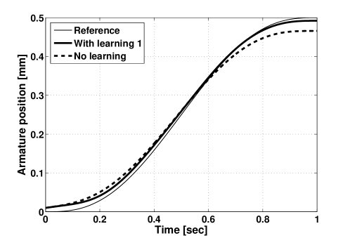
(a) Obtained armature position vs. reference trajectory - Controller (22)

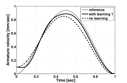
(b) Obtained armature velocity vs. reference trajectory - Controller (22)

Figure 1: Obtained outputs vs. reference trajectory - Controller (22) without learning (dashed line), with learning (bold line)

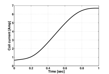
(a) Obtained coil current

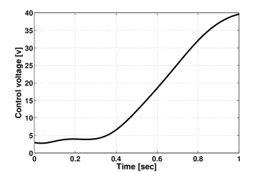
(b) Control voltage

Figure 2: Coil voltage and current - Controller (22)

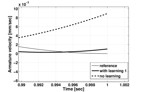
(a) Zoom at $t=t_{f}$ of the obtained armature velocity vs. reference trajectory - Controller (22) without learning (dashed line), with learning (bold line)

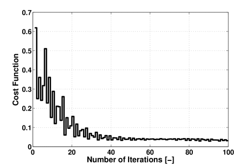
(b) Cost function vs. learning iterations

Figure 3: Impact velocity performance- Controller (22)

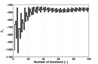
(a) $K_{1}$ vs. learning iterations

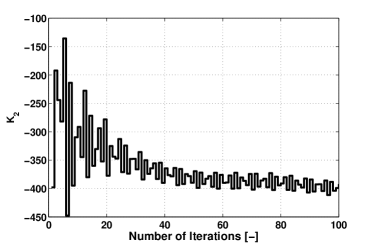
(b) $K_{2}$ vs. learning iterations

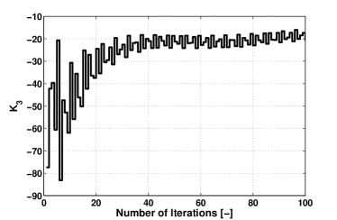
(c) $K_{3}$ vs. learning iterations

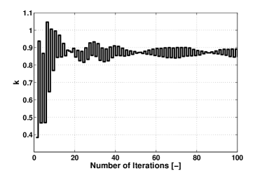
(d) $k$ vs. learning iterations

Figure 4: Gains learning- Controller (22)

VI Conclusion

In this work we have studied the problem of iterative feedback gains tuning for Input-Output linearization with static state feedback. We first used Input-Output linearization with static state feedback method and ‘robustified’ it with respect to bounded additive model uncertainties, using Lyapunov reconstruction techniques, to ensure uniform boundedness of a tracking error vector. Secondly, we complemented the Input-Output linearization controller with a model-free learning algorithm to iteratively auto-tune the control feedback gains and optimize a desired performance of the system. The learning algorithm used here is based on multi-parametric extremum seeking theory. The full controller, i.e. the learning algorithm together with the passive robust controller forms an iterative gains auto-tuning Input-Output linearization controller. We have reported some numerical results obtained on an electromagnetic actuators example. Future investigations will focuss on improving the convergence rate by using different MES algorithms with semi-global convergence properties, e.g. [21, 22, 23], extending this work to different type of model-free learning algorithms, e.g. reinforcement learning algorithms, and comparing the learning algorithms in terms of their convergence rate and achievable optimal performances.

References

- [1] A. Isidori, Nonlinear Control Systems, 2nd ed., ser. Communications and Control Engineering Series. Springer-Verlag, 1989.
- [2] L. Freidovich and H. Khalil, “Performance recovery of feedback-linearization based designs,” IEEE, Transactions on Automatic Control, vol. 53, no. 10, pp. 2324–2334, November 2008.
- [3] Y.-S. Chou and W. Wu, “Robust nonlinear control associating robust feedback linearization and H∞ control,” Chemical Enginnering Science, vol. 50, no. 9, pp. 1429–1439, 1995.
- [4] C. Pop and E. Dulf, Recent advances in robust control- Novel approaches and design methods, intech ed., 2011, ch. Robust feedback linearization control for reference tracking and disturbance rejection in nonlinear systems, pp. 274–290.
- [5] A. L. D. Franco, H. Bourl s, E. R. de Pieri, and H. Guillard, “Robust nonlinear control associating robust feedback linearization and H∞ control,” IEEE, Transactions on Automatic Control, vol. 51, no. 7, pp. 1200–1207, November 2006.
- [6] O. Lequin, M. Gevers, M. Mossberg, E. Bosmans, and L. Triest, “Iterative feedback tuning of PID parameters: comparison with classical tuning rules,” Control Engineering Practice, vol. 11, no. 9, pp. 1023 – 1033, 2003.
- [7] H. Hjalmarsson, “Iterative feedback tuning an overview,” International Journal of Adaptive Control and Signal Processing, vol. 16, no. 5, pp. 373–395, 2002. [Online]. Available: http://dx.doi.org/10.1002/acs.714
- [8] N. Killingsworth and M. Kristic, “PID tunning using extremum seeking,” IEEE Control Systems Magazine, pp. 1429–1439, 2006.
- [9] L. Koszalka, R. Rudek, and I. Pozniak-Koszalka, “An idea of using reinforcement learning in adaptive control systems,” in Networking, International Conference on Systems and International Conference on Mobile Communications and Learning Technologies, 2006. ICN/ICONS/MCL 2006. International Conference on, April 2006, pp. 190–196.
- [10] M. Benosman and G. Atinc, “Multi-parametric extremum seeking-based learning control for electromagnetic actuators,” in American Control Conference, 2013, pp. 1917–1922.
- [11] H. Khalil, Nonlinear systems, 2nd ed. New York Macmillan, 1996.
- [12] M. Benosman and K.-Y. Lum, “Passive actuators’ fault tolerant control for affine nonlinear systems,” IEEE, Transactions on Control Systems Technology, vol. 18, no. 1, pp. 152–163, January 2010.
- [13] W. M. Haddad, V. Chellaboind, and S. G. Nersesov, Impulsive and Hybrid Dynamical Systems: Stability, Dissipativity, and Control. Princeton University Press, Princeton, 2006.
- [14] H. Elmali and N. Olgac, “Robust output tracking control of nonlinear mimo systems via sliding mode technique,” Automatica, vol. 28, no. 1, pp. 145–151, 1992.
- [15] K. B. Ariyur and M. Krstic, “Multivariable extremum seeking feedback: Analysis and design,” in Proc. of the Mathematical Theory of Networks and Systems, South Bend, IN, August 2002.
- [16] Y. Wang, A. Stefanopoulou, M. Haghgooie, I. Kolmanovsky, and M. Hammoud, “Modelling of an electromechanical valve actuator for a camless engine,” in 5th International Symposium on Advanced Vehicle Control, 2000, number 93.
- [17] K. Peterson and A. Stefanopoulou, “Extremum seeking control for soft landing of electromechanical valve actuator,” Automatica, vol. 40, pp. 1063–1069, 2004.
- [18] N. Kahveci and I. Kolmanovsky, “Control design for electromagnetic actuators based on backstepping and landing reference governor,” in 5th IFAC Symposium on Mechatronic Systems, Cambridge, September 2010, pp. 393–398.
- [19] Y. Tan, D. Nesic, and I. Mareels, “On the dither choice in extremum seeking control,” Automatica, no. 44, pp. 1446–1450, 2008.
- [20] W. Moase, C. Manzie, and M. Brear, “Newton-like extremum seeking part I: Theory,” in IEEE, Conference on Decision and Control, December 2009, pp. 3839–3844.
- [21] Y. Tan, D. Nesic, and I. Mareels, “On non-local stability properties of extremum seeking control,” Automatica, no. 42, pp. 889–903, 2006.
- [22] W. Noase, Y. Tan, D. Nesic, and C. Manzie, “Non-local stability of a multi-variable extremum-seeking scheme,” in IEEE, Australian Control Conference, November 2011, pp. 38–43.
- [23] A. Scheinker, “Simultaneous stabilization of and optimization of unkown time-varying systems,” in American Control Conference, June 2013, pp. 2643–2648.