Efficient generation of twin photons at telecom wavelengths with 10 GHz repetition-rate tunable comb laser

Abstract

Efficient generation and detection of indistinguishable twin photons are at the core of quantum information and communications technology (Q-ICT). These photons are conventionally generated by spontaneous parametric down conversion (SPDC), which is a probabilistic process, and hence occurs at a limited rate, which restricts wider applications of Q-ICT. To increase the rate, one had to excite SPDC by higher pump power, while it inevitably produced more unwanted multi-photon components, harmfully degrading quantum interference visibility. Here we solve this problem by using recently developed 10 GHz repetition-rate-tunable comb laser Sakamoto et al. (2008); Morohashi et al. (2012), combined with a group-velocity-matched nonlinear crystal Jin et al. (2013a, 2014), and superconducting nanowire single photon detectors Miki et al. (2013); Yamashita et al. (2013). They operate at telecom wavelengths more efficiently with less noises than conventional schemes, those typically operate at visible and near infrared wavelengths generated by a 76 MHz Ti Sapphire laser and detected by Si detectors Lu et al. (2007); Huang et al. (2011); Yao et al. (2012). We could show high interference visibilities, which are free from the pump-power induced degradation. Our laser, nonlinear crystal, and detectors constitute a powerful tool box, which will pave a way to implementing quantum photonics circuits with variety of good and low-cost telecom components, and will eventually realize scalable Q-ICT in optical infra-structures.

I Introduction

Since the first experimental realization of quantum teleportation Bouwmeester et al. (1997), many experiments with multiphoton entanglement have been demonstrated Lu et al. (2007); Pan et al. (2012), and currently expanded to eight photons, employing multiple SPDC crystals Huang et al. (2011); Yao et al. (2012). In order to increase the scale of entanglement further, the generation probability per SPDC crystal must be drastically improved without degrading the quantum indistinguishability of photons. Unfortunately, however, a dilemma always exists in SPDC: higher pump power is required for higher generation probability, while it degrades quantum interference visibility due to unwanted multi-pair emissions, leading to the increase of error rates in entanglement-based quantum key distribution (QKD) Fujiwara et al. (2014) and photonic quantum information processing Knill et al. (2001).

When $n$ SPDC sources are used, the 2$n$-fold coincidence counts (CC) can be estimated as

$$CC=fp^{n}\eta^{2n},$$ (1)

where $f$ is the repetition rate of the pump laser, $p$ is the generation probability of one photon-pair per pulse, $\eta$ is the overall efficiency, which is the product of the collecting efficiency of the whole optical system and the detecting efficiency of the detectors. The $p$ should be restricted to less than 0.1, so that the effect of unwanted multi-pair emissions can be negligible. So the pump power is tuned for $p\leq 0.1$.

The value of $p$ is not high in the conventional photon source. A standard technology is based on SPDC at visible and near infrared wavelengths using a BBO crystal pumped by the second harmonic of the femto-second laser pulses from a Ti Sapphire laser, whose repetition rate is 76 MHz Lu et al. (2007); Huang et al. (2011); Yao et al. (2012). In this case, the probability $p$ had not been able to go beyond 0.06, because the second harmonic power was limited to 300-900 mW for a fundamental laser power of 1-3 W. Therefore, recent efforts have been focused on increasing the pump power Krischek et al. (2010).

Recently the periodically poled KTP (PPKTP) crystals attract much attention because it can achieve $p\sim$0.1 (0.6) at telecom wavelengths with a pump power of 80 (400) mW thanks to the quasi-phase matching (QPM) technique Jin et al. (2013b). When waveguide structure is employed, $p$ can be $10^{3}$ times higher than the bulk crystal Tanzilli et al. (2001); Zhong et al. (2012). Unfortunately, however, the constraint $p\leq 0.1$ should be met in these cases too. The $\eta$ is already maximized by careful alignment in laboratories, e.g., the typical $\eta$ value is about 0.2-0.3 Huang et al. (2011); Yao et al. (2012); Jin et al. (2013b). Thus $p$ and $\eta$ have almost reach their maxima. The remaining effective way is to improve the repetition rate of the pump laser, $f$.

In this work, we demonstrate a novel photon source pumped by a recently developed repetition-rate-tunable comb laser in a range of 10-0.625 GHz Sakamoto et al. (2008); Morohashi et al. (2012). This laser can operate in relatively low pulse energy, while keeping high average power, thanks to a high repetition rate. The low pulse energy would result in the reduction of the multiple-pair emission. At the same time a high counting rate would be expected owing to the high average power. The SPDC based on a group-velocity-matched PPKTP (GVM-PPKTP) crystal can achieve very high spectral purity of the constituent photons Jin et al. (2013a, 2014). Furthermore, the photons are detected by the state-of-the-art superconducting nanowire single photon detectors (SNSPDs) Miki et al. (2013); Yamashita et al. (2013), which have a much higher efficiency than that of traditional InGaAs avalanche photodiode (APD).

II Experiment

The experimental setup is shown in Fig. 1.

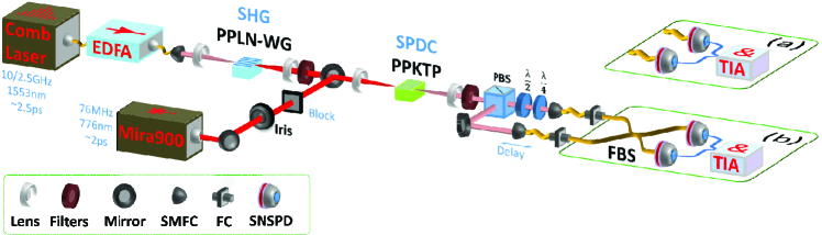
Figure 1: The Experimental setup. A comb laser with a 10-0.625 GHz tunable-repetition-rate at 1553 nm wavelength is amplified by a high-power erbium-doped fiber amplifier (EDFA), and frequency doubled by a 10-mm-long type-0 periodically poled lithium niobate wave guide (PPLN-WG, by NTT Electronics, polling period=18.2 $\mu$m). Then, after filtered by short-pass filters, the 776.5 nm laser light from second harmonic generation (SHG) pumps a 30-mm type-II periodically poled potassium titanyl phosphate crystal (PPKTP, by Raicol, poling period= 46.1 $\mu$m, temperature = $47.8\,^{\circ}\mathrm{C}$) for SPDC. The downconverted photons, the signal and idler, are filtered by long-pass filters, separated by a polarization beamsplitter (PBS), and coupled into single mode fibers (SMF) by couplers (SMFC). (a) The collected photons are directly detected by SNSPDs, which are connected to a time interval analyzer (TIA) for the measurement of Time of Arrival (ToA). (b) SMFs are connected to a fiber beamsplitter (FBS) by two fiber connectors (FC), for the test of Hong-Ou-Mandel dip. A half-wave plate and a quarter-wave plate are added to guarantee the signal and idler photons have the same polarization in FBS. For comparison, we also introduce a 76 MHz pump laser (Mira900, at 776.5 nm, around 2 ps). An iris is inserted for 76 MHz laser to make the beam waist comparable with the comb laser.

The picosecond pulses from the comb laser are generated with the following principles Sakamoto et al. (2008); Morohashi et al. (2012). A continuous-wave (cw) light emitted from a single-mode laser diode (LD) with a wavelength of around 1553 nm is led into a Mach-Zehnder-modulator (MZM) and is converted to a comb signal with 10 GHz in spacing and 300 GHz in bandwidth. The MZM is fabricated on a LiNbO₃ crystal and is driven by a 10 GHz radio-frequency signal. Because the comb signal has linear chirp, it can be formed to a picosecond pulse train with a repetition rate of 10 GHz by chirp compensation using a single-mode fiber. The comb laser also includes a pulse picker, so that the repetition frequency of the pulse train can be changed in the range of 10-0.625 GHz. In this experiment, we keep the temporal width around 2.5 ps. Fig. 2(a) shows the spectrum of this laser at 2.5 GHz repetition rate. See the Appendix for more spectral and temporal information of this comb laser. For more details of this kind of comb lasers, see Refs. Sakamoto et al. (2007); Morohashi et al. (2008).

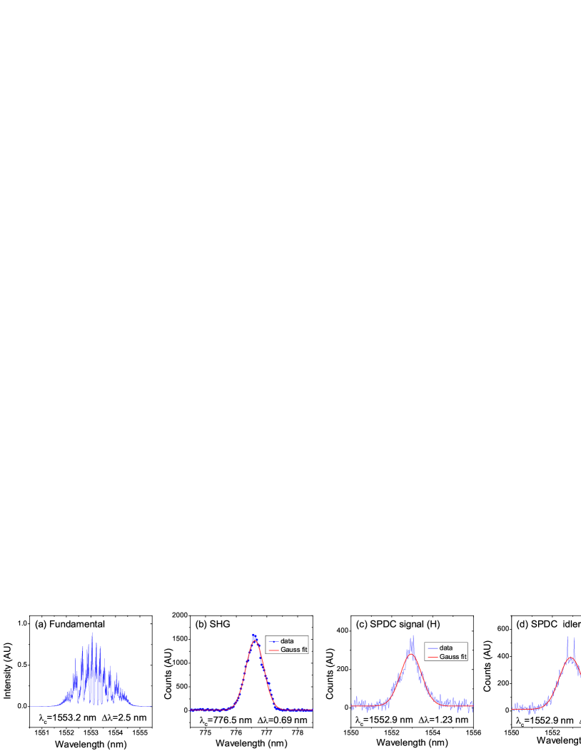
Figure 2: The spectra. (a) The spectra of the comb laser at 2.5 GHz repetition rates. (b) A typical spectrum of SHG, pumped by the fundamental laser. (c, d) Spectra of the signal (horizontal polarization) and idler (vertical polarization) photons generated in SPDC.

Generating a high-power second harmonic light (SHG) is a key point in this experiment. Since the average power per pulse of the comb laser is very low, we choose a periodically poled lithium niobate wave guide (PPLN-WG) for SHG. We tested both 10 GHz and 2.5 GHz repetition rate lasers. We found the SHG power with 2.5 GHz repetition rate was more stable than that with 10 GHz repetition rate. Therefore, the data in this experiment are mainly obtained by using 2.5 GHz repetition rate. With the input 2.5 GHz repetition rate fundamental laser at a power of 500 mW, we obtained 42 mW SHG power. After filtered by several short-pass filters to cut the fundamental light, we finally achieved a net SHG power of 35 mW. The transmission loss of the PPLN-WG was around 50%. Fig. 2(b) is the spectrum of 776.5nm SHG laser, measured by a spectrometer (SpectraPro-2300i, Acton Research Corp.). Interestingly, it can be noticed that the comb structure no-longer exists in the SHG spectrum, which may be caused by a sum-frequency-generation process.

For SPDC, the nonlinear crystal used in this experiment is a PPKTP crystal, which satisfy the GVM condition at telecom wavelength Jin et al. (2013a); König and Wong (2004); Evans et al. (2010); Gerrits et al. (2011); Eckstein et al. (2011). Thanks to the GVM condition, the spectral purity is much higher at telecom wavelength than that at visible wavelengths Jin et al. (2014). This spectrally pure photon source is very useful for multi-photon interference between independent sources Mosley et al. (2008); Jin et al. (2011, 2013c). Figure 2(c, d) are the observed spectra of the signal and idler photons, measured by a spectrometer (SpctraPro-2500i, Acton Research Corp.). The FWHMs of the twin photons are about 1.2-1.3 nm, similar as the spectral width of the photons pumped by 76 MHz laser Jin et al. (2013a).

Our superconducting nanowire single photon detectors (SNSPDs) have a system detection efficiency (SDE) of around 70% with a dark count rate (DCR) less than 1 kcps Miki et al. (2013); Yamashita et al. (2013); Jin et al. (2013b). The SNSPD also has a wide spectral response range that covers at least from 1470 nm to 1630 nm wavelengths Jin et al. (2013b). The measured timing jitter and dead time (recovery time) were 68 ps Miki et al. (2013) and 40 ns Miki et al. (2007).

The performance with the 2.5 GHz source is evaluated in terms of a signal to noise ratio (SNR) Broome et al. (2011) and a Hong-Ou-Mandel (HOM) interference Hong et al. (1987), in comparison with the 76 MHz laser. The SNR test is carried out in the detecting configuration of Fig. 1(a), while the HOM test is performed in that of Fig. 1(b).

III Result 1: Signal to noise ratio test

The SNR is defined as the ratio of single pair emission rate over the double pair emission rate Broome et al. (2011). These rates can be evaluated by Time of Arrival (ToA) data, which are shown in Fig. 3(a-d).

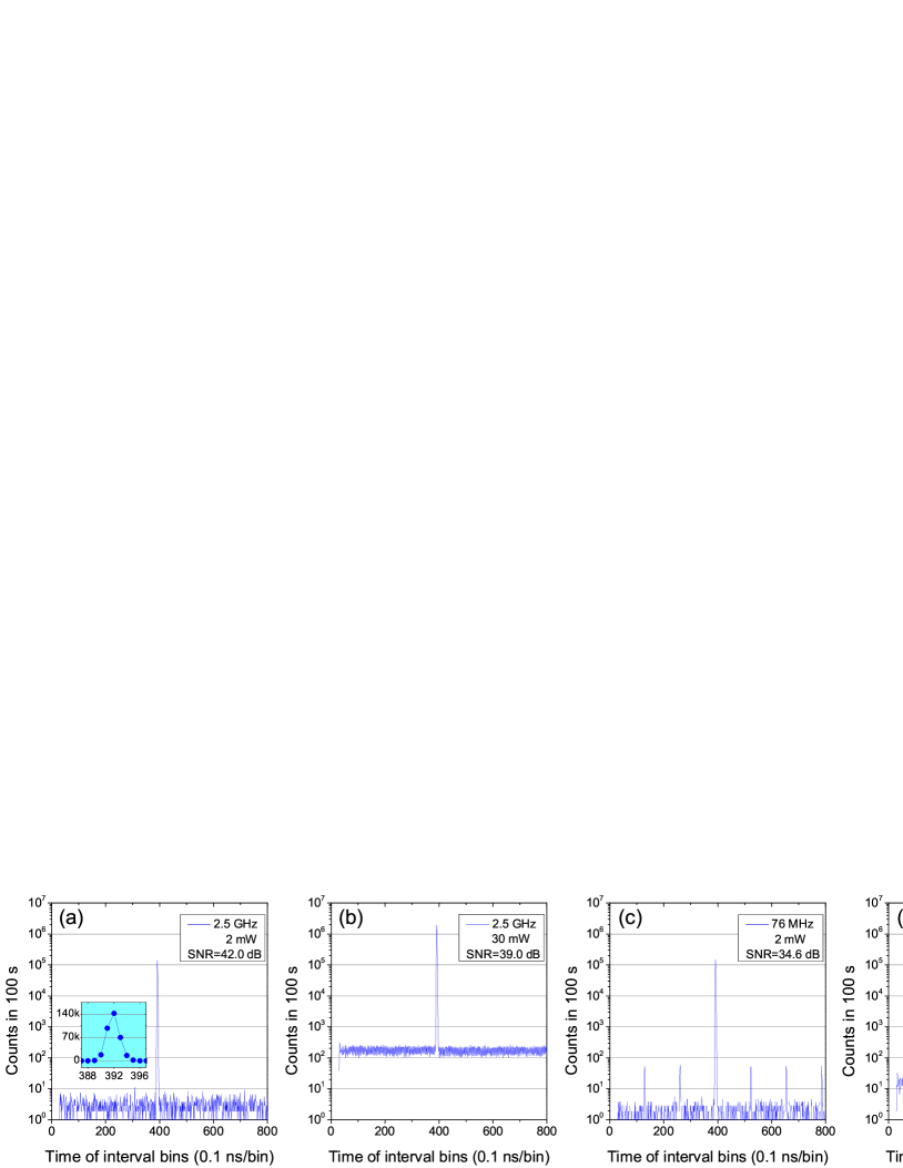
Figure 3: Time of Arrival (ToA) data. The data in each figure was accumulated in 100 seconds for 2.5 GHz and 76 MHz lasers at 2 mW and 30 mW. The peak intervals are 0.4 ns in (a, b) and 13.1 ns in (c, d). The measured SNR values are 42.0 dB, 39.0 dB, 34.6 dB and 23.0 dB for (a-d), respectively. Inset in (a) is an enlarged view of the main peak in a linear scale.

Each data consists of the main peak and side peaks, and we define the peak counts as the value of each peak. The side peaks are not visible in Fig. 3(a, b) because the resolution of the detector system ($\sim$0.5 ns, as seen in the inset in (a)) is comparable to the pulse interval of 2.5 GHz laser (0.4 ns). So, we set the averaged maximal counts as the side peak values. The side peaks are recorded when a second SPDC occurs (in the stop channel) conditioned on a first SPDC (in the start channel) occurs at the main peaks. Therefore, the side peaks correspond to the rate of 2-pair components in SPDC, while the main peaks correspond to the rate of 1-pair plus 2-pair components in SPDC. So the SNR can be calculated in dB as

$$SNR=10\log_{10}{[(\text{main peak}-\text{side peak})/\text{side peak}]}.$$ (2)

The measured SNR are 42.0 dB, 39.0 dB, 34.6 dB, 23.0 dB for Fig. 3(a-d), respectively.

Theoretical calculation unveils that the SNR is proportional to the inverse of average photon numbers per pulse at a lower pump power Broome et al. (2011). This claim can be experimentally verified by comparing Fig. 3(c) and (d) with the 76 MHz laser. When the pump power increases from 2 mW to 30 mW, the SNR is decreased by 34.6 - 23.0 = 11.6 dB. It agrees well with the 30 mW / 2 mW = 15 times (11.7 dB) increase of average photon number per pulse.

Next, we compare the result in Fig. 3(b) and (d), so as to confirm the validity of the definition for side peak values in Fig. 3(a) and (b). At 30 mW pump power, the coincidence counts are 48 kcps and 56 kcps for 2.5 GHz and 76 MHz laser, respectively, as seen from Fig. 3(b) and (d). Then the average photon numbers per pulse are estimated to be 0.00021 and 0.0079, correspondingly. The average photon pair per pulse for the 2.5 GHz laser is 0.0079 / 0.00021 = 37.6 times (15.8 dB) lower than that of the 76 MHz laser. Recall the SNR difference between 2.5 GHz and 76 MHz of 39.0 - 23.0 = 16.0 dB. This consistency verifies the validity of the definition for side peak values in Fig. 3(a) and (b).

Finally, we estimate the SNR values for the case of the 2.5 GHz laser at 2 mW in Fig. 3(a). The SNR at 2 mW should ideally increase by 11.7 dB (15 times), from 39.0 dB (30 mW in Fig. 3(b)) to 50.7 dB. Actually, however, the measured SNR is only 42.0 dB. This discrepancy is mainly due to the dark counts by the detectors and the accidental counts by stray photons.

IV Result 2: Hong-Ou-Mandel interference test

We then carried out the HOM interference test to evaluate the performance of a twin photon source. We firstly worked with 30 mW pump power for 2.5 GHz and 76 MHz repetition rate lasers, and achieved raw visibilities of 96.4 $\pm$ 0.2% and 95.9 $\pm$ 0.1%, respectively, as shown in Fig. 4(a, b).

Figure 4: Hong-Ou-Mandel (HOM) dip. HOM dip for 2.5 GHz (a) and 76 MHz (b) repetition rate lasers with pump power of 30 mW, fitted with triangle shape function.

The triangle-shape of the HOM dip in Fig. 4(a, b) is caused by the group-velocity matching condition in PPKTP crystal at telecom wavelengths Kuzucu et al. (2005); Shimizu and Edamatsu (2009). The widths of the dips in Fig. 4 (a, b) are similar, around 1.33 mm (4.4 ps), since the width of the dip is determined by the length of the crystal Ansari et al. (2014). The high visibilities in Fig. 4 confirmed the high indistinguishability of the generated photons.

To compare the different performance of the 2.5 GHz and 76 MHz lasers, we repeated the HOM interference test at different pump powers. Without subtract any background counts, we compare the raw visibilities of HOM dip at different pump powers in Fig. 5.

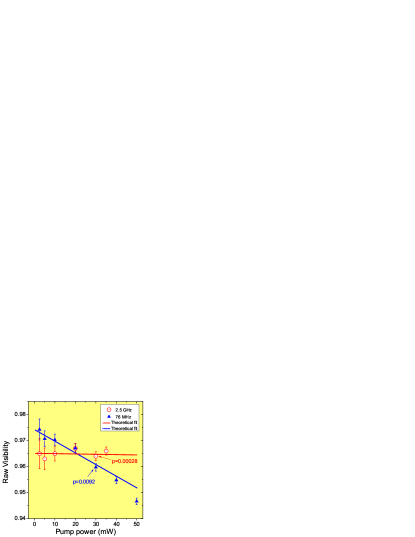
Figure 5: Raw visibilities versus pump powers for 2.5 GHz and 76 MHz lasers. At 30 mW, the average photon numbers per pulse were 0.00028 and 0.0092 for 2.5 GHz and 76 MHz lasers. The uncertainties of these visibilities were derived using Poissonian errors on the coincidence counts. The solid lines are the theoretical fit.

At a low pump power of 2.5 mW, the 76 MHz laser has a visibility of 97.4 $\pm$ 0.4%, slightly higher than the result by the 2.5 GHz laser, 96.5 $\pm$0.6%. At 30 mW, the average photon numbers per pulse were 0.00028 and 0.0092 for 2.5 GHz and 76 MHz lasers. Note the average photon numbers per pulse in the HOM interference test were slightly higher than that in the ToA test, because we slightly improved the experimental condition in the test of HOM interference.

It is noteworthy that the visibilities by the 76 MHz laser decrease rapidly when the pump powers increase. In contrast, the visibilities by the 2.5 GHz laser shows almost no decrease up to 35 mW, the maximum SHG power we have achieved in experiment. To fit this experimental data, we construct a theoretical model. In this model, the transmittance loss of the signal and idler photons are effectively described by two beam splitters, and the mode-matching efficiency $\eta_{M}$ between the signal and idler are also represented by two beam splitters with the transmittance of $\eta_{M}$. The transmittance loss is obtained from the experimental condition, while the mode-matching efficiency are searched so as to fit the experimental data. The numerical analyses suggest that the HOM visibility is extremely sensitive to the mode matching efficiency, $\eta_{M}$. However, it is not easy to estimate the experimental $\eta_{M}$ value with enough accuracy. In Fig. 5, the data are fitted with $\eta_{M}$ values of 0.9828 and 0.9878 for 2.5 GHz laser and 76 MHz laser, respectively. Higher $\eta_{M}$ value for the 76 MHz laser is reasonable, because the indistinguishablites of the twin photons generated by the 76 MHz laser is slightly better than that by the 2.5 GHz laser, which can be roughly checked by the spectra of the signal and idler in Fig. 2(c) and (d). After the transmittance efficiency and the mode-matching efficiency are fixed, the HOM visibilities are only determined by $p$, the average photon pairs per pulse (i.e., the generation probability of one pair per pulse). The low value $p$ by the 2.5 GHz laser guarantees its high visibilities at high pump powers. In Fig. 5, the theoretical model fitted well with our experimental data. See more details of our model in the Appendix.

V Discussion and Outlook

With the theoretical model (See the Appendix), we further calculate the visibilities at high pump powers, as shown in Tab. 1. It is interesting to note that, at high pump power up to 3 W, the visibility by 76 MHz laser will decrease to 62.4%, while the 2.5 GHz laser still can keep the visibility higher than 90 %, mainly thanks to the low average photon numbers per pulse. To experimentally demonstrate this high visibilities at high pump powers in the future, we could update the PPKTP bulk crystal to a PPKTP waveguide. Also, SHG power of the comb laser at 10 GHz repetition rate needs to be improved. See the Appendix for the HOM interference of this comb laser at 10 GHz repetition rate.

	30 mW	$\sim$300 mW	$\sim$3 W
76 MHz	0.0092 (96.1%)	0.092 (86.1%)	0.92 (62.4%)
2.5 GHz	0.00028 (96.4%)	0.0028 (96.0%)	0.028 (91.8%)

Table 1: Visibilities at high pump powers. The estimated average photon pairs per pulse and the corresponding visibilites at different pump powers for 76 MHz and 2.5 GHz laser. The visibilities are directly determined by the average photon pairs per pulse.

Nevertheless, our experimental results in Fig. 5 have clearly shown the non-degradation of HOM visibilites at high pump powers.

We notice that many other schemes have been reported to reduce the multi-pair emission. Broome et al demonstrated to reduce the multi-pair emission by temporally multiplexing the pulsed pump lasers by two times Broome et al. (2011). Ma et al tried to reduce such effects by multiplexing four independent SPDC sources Ma et al. (2011). All the previous methods have a limited effect, because the units they multiplexed were limited. If they increase the multiplexed units, the setup will be very complex. The GHz-repetition-rate-laser pumped photon source in our scheme provide a very simple and effective way to reduce the multi-pair emission. In addition, GHz repetition rate lasers are now commercially available Morris et al. (2014); Gig ; M2l .

Therefore, our scheme will be a reasonable option to construct the next generation of twin photon sources with high brightness, low multi-pair emission and high detection efficiency. In the traditional twin photon source technologies, 76 MHZ pump laser is compatible with a BBO crystal (with maximum $p\sim 0.06$, corresponding to photon pair generation rate of 5 MHz) and Si avalanche photodiode (with acceptable maximal photon numbers of 5-10 MHz). In the next generation of twin photon sources, the 10 GHz laser should be combined with a high efficiency crystals, e.g., PPKTP crystal (or waveguide, with maximum $p\sim 0.1$, corresponding to photon pair generation rate of 1 GHz), and high speed detectors, e.g., the SNSPD (with acceptable maximal photon numbers of 25-100 MHz). Consequently, we expect more than tenfold brighter photon source in conjunction with both low multiple photon pairs production and high spectral purity. Further, a repetition tunability allow us to obtain an optimal generation probability in a pulse without sacrificing a photon counting rate.

VI Conclusion

We have demonstrated a twin photon source pumped by a 10-GHz-repetition-rate tunable comb laser. The photons are generated from GVM-PPKTP crystal and detected by highly efficient SNSPDs. The SNR test and HOM interference test with 2.5 GHz laser showed a high SNR and high visibilities not degrading at high pump powers, much higher than that pumped by the 76 MHz laser. The high-repetition-rate pump laser, the GVM-PPKTP crystal, and the highly efficient detectors constitute a powerful tool box at the telecom wavelengths. We believe our tool box may have a variety of applications in the future quantum infromantion and communiction technologies.

Appendix-I

In this part we provide more information of the comb laser at 10 GHz and 2.5 GHz repetition rates. Figure 6 compares the spectra, autocorrelation, and temporal sequences of the comb laser at 10 GHz and 2.5 GHz repetition rates. Figure 7 shows the Hong-Ou-Mandel dip for the comb laser at 10 GHz, with a similar bandwidth and visibility as the results by the laser at 2.5 GHz repetition rate.

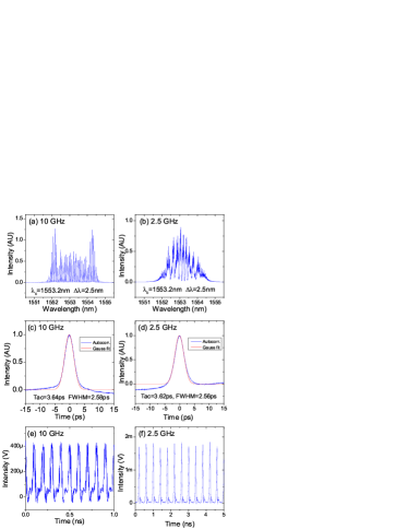
Figure 6: (a-f) The spectra, autocorrelation, and temporal sequences of the comb laser at 10 GHz and 2.5 GHz repetition rates. The full-width-at-half-maximum (FWHM) of the autocorrelation data are round 3.6 ps, corresponding to FWHM of 2.6 ps for the fundamental lasers.

Figure 7: Hong-Ou-Mandel dip for comb laser at 10 GHz repetition rate, fitted with triangle shape function. The pump power is 2 mW.

Appendix-II

In this part, we numerically analyze the relationship between photon-pair generation rate (i.e., average photon pair per pulse) and HOM interference visibility.

VI.1 The model

Here, we describe a numerical model of the HOM experiment. The model is described in Fig. 8(a) (without delay) and (b) (with delay) where $\eta_{A,B}$ represent transmittances of mode $A$ and $B$ (losses are effectively described by beam splitters), respectively, and $\eta_{D_{1}}$ and $\eta_{D_{2}}$ are the detector efficiencies. The mode mismatch between the signal and idler pulses is directly reflected to the HOM interference visibility. In our model, the mode matching efficiency $\eta_{M}$ is effectively represented by two beam splitters with the transmittance $\eta_{M}$ and extra modes $E$ and $F$.

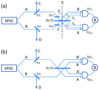
Figure 8: Models. (a) No delay (HOM dip). The mode mismatch at the 50/50 beam splitter is represented by the beam splitters $\eta_{M}$. (b) With delay. The delay is represnted by the spatial difference at the 50/50 beam splitter.

The HOM interference visibility is defined as

$$V=\frac{CC_{\rm mean}-CC_{\rm min}}{CC_{\rm mean}},$$ (3)

where $CC_{\rm min}$ and $CC_{\rm mean}$ are the coincidence count rates with zero-delay and large delay (i.e., with and without interference between the signal and idler), respectively. In the following we derive $CC_{\rm min}$ and $CC_{\rm mean}$ separately from our model.

The initial state from the SPDC source is given by a two-mode squeezed-vacuum state

$$|\psi\rangle_{AB}=\sqrt{1-\lambda^{2}}\sum_{n=0}^{\infty}\lambda^{n}|n\rangle_{A}|n\rangle_{B},$$ (4)

where $\lambda$ is the squeezing parameter, and $\lambda^{2}/(1-\lambda^{2})=p$ is the average photon pairs per pulse. Let $\hat{V}_{A(B)}^{\eta}$ be a beam splitting operator on mode $A(B)$ with transmittance $\eta$ which transforms the photon number states $|n_{1}\rangle|n_{2}\rangle$ as

$$\hat{V}_{AB}^{\eta}|n_{1}\rangle|n_{2}\rangle = \frac{1}{\sqrt{n_{1}!n_{2}!}}\sum_{k_{1}=0}^{n_{1}}\sum_{k_{2}=0}^{n_{2}}\binom{n_{1}}{k_{1}}\binom{n_{2}}{k_{2}}(-1)^{k_{2}}$$ (5)

$$\times\sqrt{\eta}^{n_{2}+k_{1}-k_{2}}\sqrt{1-\eta}^{n_{1}-k_{1}+k_{2}}$$

$$\times\sqrt{(k_{1}+k_{2})!(n_{1}+n_{2}-k_{1}-k_{2})!}$$

$$\times\left|{k_{1}+k_{2}}\right\rangle\left|{n_{1}+n_{2}-k_{1}-k}\right\rangle.$$

Applying the beam splitters $\hat{V}^{\eta_{A}}_{AC}$, $\hat{V}^{\eta_{B}}_{BD}$, $\hat{V}^{\eta_{M}}_{AE}$, $\hat{V}^{\eta_{M}}_{BF}$, and $\hat{V}^{1/2}_{AB}$ onto the two-mode squeezed vacuum (state at X in Fig. 8(a)), we obtain

$$\hat{V}^{1/2}_{AB}\hat{V}^{\eta_{M}}_{BF}\hat{V}^{\eta_{M}}_{AE}\hat{V}^{\eta_{B}}_{BD}\hat{V}^{\eta_{A}}_{AC}|\psi\rangle_{AB}|0\rangle_{C}|0\rangle_{D}|0\rangle_{E}|0\rangle_{F}$$

$$=\sqrt{1-\lambda^{2}}\sum_{n=0}^{\infty}\lambda^{n}\sum_{k_{1}=0}^{n}\binom{n}{k_{1}}^{1/2}\eta_{A}^{k_{1}/2}(1-\eta_{A})^{\frac{n-k_{1}}{2}}\sum_{k_{2}=0}^{n}\binom{n}{k_{2}}^{1/2}\eta_{B}^{k_{2}/2}(1-\eta_{B})^{\frac{n-k_{2}}{2}}$$

$$\quad\times\sum_{k_{3}=0}^{k_{1}}\binom{k_{1}}{k_{3}}^{1/2}\eta_{M}^{k_{3}/2}(1-\eta_{M})^{\frac{k_{1}-k_{3}}{2}}\sum_{k_{4}=0}^{k_{2}}\binom{k_{2}}{k_{4}}^{1/2}\eta_{M}^{k_{4}/2}(1-\eta_{M})^{\frac{k_{2}-k_{4}}{2}}$$

$$\quad\times\sum_{k_{5}=0}^{k_{3}}\sum_{k_{6}=0}^{k_{4}}\binom{k_{3}}{k_{5}}\binom{k_{4}}{k_{6}}\left(\frac{1}{2}\right)^{\frac{k_{3}+k_{4}}{2}}(-1)^{k_{6}}\left(\frac{(k_{5}+k_{6})!\,(k_{3}+k_{4}-k_{5}-k_{6})!}{k_{3}!\,k_{4}!}\right)^{1/2}$$

$$\quad\times|k_{5}+k_{6}\rangle_{A}|k_{3}+k_{4}-k_{5}-k_{6}\rangle_{B}|n-k_{1}\rangle_{C}|n-k_{2}\rangle_{D}|k_{1}-k_{3}\rangle_{E}|k_{2}-k_{4}\rangle_{F}$$

$$=\sqrt{1-\lambda^{2}}\sum_{n=0}^{\infty}\lambda^{n}\sum_{k_{1}=0}^{n}\binom{n}{k_{1}}^{1/2}\eta_{A}^{k_{1}/2}(1-\eta_{A})^{\frac{n-k_{1}}{2}}\sum_{k_{2}=0}^{n}\binom{n}{k_{2}}^{1/2}\eta_{B}^{k_{2}/2}(1-\eta_{B})^{\frac{n-k_{2}}{2}}$$

$$\quad\times\sum_{k_{3}=0}^{k_{1}}\binom{k_{1}}{k_{3}}^{1/2}\eta_{M}^{k_{3}/2}(1-\eta_{M})^{\frac{k_{1}-k_{3}}{2}}\sum_{k_{4}=0}^{k_{2}}\binom{k_{2}}{k_{4}}^{1/2}\eta_{M}^{k_{4}/2}(1-\eta_{M})^{\frac{k_{2}-k_{4}}{2}}\left(\frac{1}{2}\right)^{k_{3}+k_{4}}$$

$$\quad\times\sum_{l=0}^{k_{3}+k_{4}}\sum_{k_{5}=\max\{0,l-k_{4}\}}^{\min\{l,k_{3}\}}(-1)^{l-k_{5}}\left\{\binom{k_{3}}{k_{5}}\binom{k_{4}}{l-k_{5}}\binom{l}{k_{5}}\binom{k_{3}+k_{4}-l}{k_{3}-k_{5}}\right\}^{1/2}$$

$$\quad\times|l\rangle_{A}|k_{3}+k_{4}-l\rangle_{B}|n-k_{1}\rangle_{C}|n-k_{2}\rangle_{D}|k_{1}-k_{3}\rangle_{E}|k_{2}-k_{4}\rangle_{F},$$ (6)

where $l=k_{5}+k_{6}$ and we have used the relation

$$\binom{k_{3}}{k_{5}}\binom{k4}{k_{6}}\left(\frac{(k_{5}+k_{6})!\,(k_{3}+k_{4}-k_{5}-k_{6})!}{k_{3}!\,k_{4}!}\right)^{1/2}=\left\{\binom{k_{3}}{k_{5}}\binom{k4}{k_{6}}\binom{k_{5}+k_{6}}{k_{5}}\binom{k_{3}+k_{4}-k_{5}-k_{6}}{k_{3}-k_{5}}\right\}^{1/2}.$$ (7)

Note that $\hat{V}^{1/2}$ should be applied to mode $E$ and $F$, which will be discussed later. From Eq. (VI.1) we find the joint probability of having $l$, $k_{3}+k_{4}-l$, $n-k_{1}$, $n-k_{2}$, $k_{1}-k_{3}$, $k_{2}-k_{4}$ photons in mode A-F at X:

$$P^{X}_{ABCDEF}(l,k_{3}+k_{4}-l,n-k_{1},n-k_{2},k_{1}-k_{3},k_{2}-k_{4})$$

$$=(1-\lambda)^{2}\lambda^{2n}\eta_{A}^{k_{1}}(1-\eta_{A})^{n-k_{1}}\eta_{B}^{k_{2}}(1-\eta_{B})^{n-k_{2}}\eta_{M}^{k_{3}+k_{4}}(1-\eta_{M})^{k_{1}+k_{2}-k_{3}-k_{4}}\left(\frac{1}{2}\right)^{k_{3}+k_{4}}\binom{n}{k_{1}}\binom{n}{k_{2}}\binom{k_{1}}{k_{3}}\binom{k_{2}}{k_{4}}$$

$$\quad\times\left\{\sum_{k_{5}=\max\{0,l-k_{4}\}}^{\min\{l,k_{3}\}}(-1)^{l-k_{5}}\left\{\binom{k_{3}}{k_{5}}\binom{k_{4}}{l-k_{5}}\binom{l}{k_{5}}\binom{k_{3}+k_{4}-l}{k_{3}-k_{5}}\right\}^{1/2}\right\}^{2}.$$ (8)

The 50/50 beam splitting of mode $E$ ($F$) into $E_{A}$ and $E_{B}$ ($F_{A}$ and $F_{B}$) adds extra binomial distribution terms $\binom{k_{1}-k_{3}}{k_{7}}\binom{k_{2}-k_{4}}{k_{8}}\left(\frac{1}{2}\right)^{k_{1}+k_{2}-k_{3}-k_{4}}$ to Eq. (VI.1). The joint probability distribution for the state at the detectors is thus given by

$$P_{ABCDE_{A}F_{A}E_{B}F_{B}}(l,k_{3}+k_{4}-l,n-k_{1},n-k_{2},k_{7},k_{2}-k_{4}-k_{8},k_{1}-k_{3}-k_{7},k_{8})$$

$$=(1-\lambda)^{2}\lambda^{2n}\eta_{A}^{k_{1}}(1-\eta_{A})^{n-k_{1}}\eta_{B}^{k_{2}}(1-\eta_{B})^{n-k_{2}}\eta_{M}^{k_{3}+k_{4}}(1-\eta_{M})^{k_{1}+k_{2}-k_{3}-k_{4}}\left(\frac{1}{2}\right)^{k_{1}+k_{2}}\binom{n}{k_{1}}\binom{n}{k_{2}}\binom{k_{1}}{k_{3}}\binom{k_{2}}{k_{4}}$$

$$\quad\times\binom{k_{1}-k_{3}}{k_{7}}\binom{k_{2}-k_{4}}{k_{8}}\left\{\sum_{k_{5}=\max\{0,l-k_{4}\}}^{\min\{l,k_{3}\}}(-1)^{l-k_{5}}\left\{\binom{k_{3}}{k_{5}}\binom{k_{4}}{l-k_{5}}\binom{l}{k_{5}}\binom{k_{3}+k_{4}-l}{k_{3}-k_{5}}\right\}^{1/2}\right\}^{2}.$$ (9)

The coincidence rate $CC_{\rm min}$ is then obtained by the sum of the joint probability:

$$CC_{\rm min} = \sum_{n=0}^{\infty}\sum_{k_{1}=0}^{n}\sum_{k_{2}=0}^{n}\sum_{k_{3}=0}^{k_{1}}\sum_{k_{4}=0}^{k_{2}}\sum_{k_{7}=0}^{k_{1}-k_{3}}\sum_{k_{8}=0}^{k_{2}-k_{4}}\sum_{l=0}^{k_{3}+k_{4}}\left\{1-(1-\eta_{D_{1}})^{l+k_{2}-k_{4}+k_{7}-k_{8}}\right\}\left\{1-(1-\eta_{D_{2}})^{-l+k_{1}+k_{4}-k_{7}+k_{8}}\right\}$$ (10)

$$\times P_{ABCDE_{A}F_{A}E_{B}F_{B}}(l,k_{3}+k_{4}-l,n-k_{1},n-k_{2},k_{7},k_{2}-k_{4}-k_{8},k_{1}-k_{3}-k_{7},k_{8}).$$

The derivation of $CC_{\rm mean}$ is rather simple since there is no interference at the 50/50 beam splitter due to the delay. This is illustrated in Fig. 8(b). Note that we do not need $\eta_{M}$. The two-mode squeezed vacuum from the SPDC source has a joint photon distribution:

$$P_{AB}(n,n)=(1-\lambda^{2})\lambda^{2n}.$$ (11)

The beam splitting operation simply spread this distribution in a binomial manner. For example, after the beam splitter $\eta_{A}$, the joint distribution is given by

$$P_{ABC}(n,k_{1},n-k_{1})=(1-\lambda^{2})\lambda^{2n}\binom{n}{k_{1}}\eta_{A}^{k_{1}}(1-\eta_{A})^{n-k_{1}}.$$ (12)

Applying the $\eta_{B}$ and 50/50 beam splitters in a similar way, we have

$$P_{AA^{\prime}BB^{\prime}CD}(k_{3},k_{2}-k_{4},k_{4},k_{1}-k_{3},n-k_{1},n-k_{2})$$

$$=(1-\lambda^{2})\lambda^{2n}\binom{n}{k_{1}}\binom{n}{k_{2}}\binom{k_{1}}{k_{3}}\binom{k_{2}}{k_{4}}\eta_{A}^{k_{1}}(1-\eta_{A})^{n-k_{1}}\eta_{B}^{k_{2}}(1-\eta_{B})^{n-k_{2}}\left(\frac{1}{2}\right)^{k_{1}+k_{2}},$$ (13)

before the detectors. The coincidence count $CC_{\rm mean}$ is then given by

$$CC_{\rm mean} = \sum_{n=0}^{\infty}\sum_{k_{1}=0}^{n}\sum_{k_{2}=0}^{n}\sum_{k_{3}=0}^{k_{1}}\sum_{k_{4}=0}^{k_{2}}\left\{1-(1-\eta_{D_{1}})^{k_{2}+k_{3}-k_{4}}\right\}\left\{1-(1-\eta_{D_{2}})^{k_{1}-k_{3}+k_{4}}\right\}$$ (14)

$$\times P_{AA^{\prime}BB^{\prime}CD}(k_{3},k_{2}-k_{4},k_{4},k_{1}-k_{3},n-k_{1},n-k_{2}).$$

The HOM visibility in Eq. (3) is thus calculable from Eqs. (10) and (14).

VI.2 Numerical result

The transmittances (efficiencies) of each components in the experiment are summarized in Table 2 (see Fig. 8 for the theoretical model and the corresponding experimental setup in Main text. In fact, the HOM visibility is extremely sensitive to the mode matching factor $\eta_{M}$. It is however not easy to estimate the mode matching factor $\eta_{M}$ experimentally with enough accuracy.

In Fig. 9, we plot the numerical results with various $\eta_{M}$, and the experimental data with the 76 MHz laser. The experimental average photon-pair $p$ is estimated from the experimental count rates. The experimental data fit the theoretical lines well within $0.9848\leq\eta_{M}\leq 0.9888$. With the parameters in Table 2, we also calculated the performance of our scheme at high photon-pair generation rate, as shown in Fig. 10 and Table 3. From this simulation, we find several interesting relationship. (1), The visibility is directly determined by the average photon-pairs. (2), The slope of this line is very sensitive to the unbalanced loss in the delay arm and non-delay arm. (3), The Y-intercept of this line very sensitive to the mode matching efficiency.

Table 2: Transmittance and efficiency of the components in the experiment. SMFC: single mode fiber coupler. FC: fiber connector. SNSPD: superconducting nanowier single photon detector.

$\eta_{A}$	0.42	SMFC + FCs
$\eta_{B}$	0.29	SMFC + FCs + Delay line
$\eta_{D_{1}}$	0.68	SNSPD1
$\eta_{D_{2}}$	0.70	SNSPD2

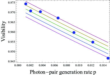
Figure 9: The HOM visibility versus $p$. The solid lines represent theoretical curves with $\eta_{M}=0.9888,0.9878,0.9868,0.9858,0.9848$ from the top to the bottom. The plots are the experimental results with the 76 MHz laser.

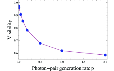
Figure 10: The HOM visibilities at different $p$ values, with $\eta_{M}=0.9878$.

Table 3: The visibilities at different photon-pair generation rate.

$p$	0.001	0.005	0.01	0.05	0.1	0.2	0.5	1	2
V	0.974	0.968	0.960	0.906	0.854	0.781	0.677	0.618	0.585

References

- Sakamoto et al. (2008) T. Sakamoto, T. Kawanishi, and M. Tsuchiya, Opt. Lett. 33, 890 (2008).
- Morohashi et al. (2012) I. Morohashi, M. Oikawa, Y. Tamura, S. Aoki, T. Sakamoto, T. Kawanishi, and I. Hosako, in Conference on Lasers and Electro-Optics 2012 (Optical Society of America, 2012) p. CF1N.7.
- Jin et al. (2013a) R.-B. Jin, R. Shimizu, K. Wakui, H. Benichi, and M. Sasaki, Opt. Express 21, 10659 (2013a).
- Jin et al. (2014) R.-B. Jin, R. Shimizu, K. Wakui, M. Fujiwara, T. Yamashita, S. Miki, H. Terai, Z. Wang, and M. Sasaki, Optics Express, Opt. Express 22, 11498 (2014).
- Miki et al. (2013) S. Miki, T. Yamashita, H. Terai, and Z. Wang, Opt. Express 21, 10208 (2013).
- Yamashita et al. (2013) T. Yamashita, S. Miki, H. Terai, and Z. Wang, Optics Express, Opt. Express 21, 27177 (2013).
- Lu et al. (2007) C.-Y. Lu, X.-Q. Zhou, O. Guhne, W.-B. Gao, J. Zhang, Z.-S. Yuan, A. Goebel, T. Yang, and J.-W. Pan, Nat. Phys. 3, 91 (2007).
- Huang et al. (2011) Y.-F. Huang, B.-H. Liu, L. Peng, Y.-H. Li, L. Li, C.-F. Li, and G.-C. Guo, Nat. Commun. 2, 546(1 (2011).
- Yao et al. (2012) X.-C. Yao, T.-X. Wang, P. Xu, H. Lu, G.-S. Pan, X.-H. Bao, C.-Z. Peng, C.-Y. Lu, Y.-A. Chen, and J.-W. Pan, Nat. Photon. 6, 225 (2012).
- Bouwmeester et al. (1997) D. Bouwmeester, J.-W. Pan, K. Mattle, M. Eibl, H. Weinfurter, and A. Zeilinger, Nature 390, 575 (1997).
- Pan et al. (2012) J.-W. Pan, Z.-B. Chen, C.-Y. Lu, H. Weinfurter, A. Zeilinger, and M. Żukowski, Rev. Mod. Phys. 84, 777 (2012).
- Fujiwara et al. (2014) M. Fujiwara, K.-i. Yoshino, Y. Nambu, T. Yamashita, S. Miki, H. Terai, Z. Wang, M. Toyoshima, A. Tomita, and M. Sasaki, Optics Express, Opt. Express 22, 13616 (2014).
- Knill et al. (2001) E. Knill, R. Laflamme, and G. J. Milburn, Nature 409, 46 (2001).
- Krischek et al. (2010) R. Krischek, W. Wieczorek, A. Ozawa, N. Kiesel, P. Michelberger, T. Udem, and H. Weinfurter, Nat. Photon. 4, 170 (2010).
- Jin et al. (2013b) R.-B. Jin, M. Fujiwara, T. Yamashita, S. Miki, H. Terai, Z. Wang, K. Wakui, R. Shimizu, and M. Sasaki, arXiv:1309.1221 (2013b).
- Tanzilli et al. (2001) S. Tanzilli, H. de Riedmatten, H. Tittel, H. Zbinden, P. Baldi, M. De Micheli, D. B. Ostrowsky, and N. Gisin, Electronics Letters, Electron. Lett. 37, 26 (2001).
- Zhong et al. (2012) T. Zhong, F. N. C. Wong, A. Restelli, and J. C. Bienfang, Opt. Express 20, 26868 (2012).
- Sakamoto et al. (2007) T. Sakamoto, T. Kawanishi, and M. Izutsu, Opt. Lett. 32, 1515 (2007).
- Morohashi et al. (2008) I. Morohashi, T. Sakamoto, H. Sotobayashi, T. Kawanishi, I. Hosako, and M. Tsuchiya, Opt. Lett. 33, 1192 (2008).
- König and Wong (2004) F. König and F. N. C. Wong, Appl. Phys. Lett. 84, 1644 (2004).
- Evans et al. (2010) P. G. Evans, R. S. Bennink, W. P. Grice, T. S. Humble, and J. Schaake, Phys. Rev. Lett. 105, 253601 (2010).
- Gerrits et al. (2011) T. Gerrits, M. J. Stevens, B. Baek, B. Calkins, A. Lita, S. Glancy, E. Knill, S. W. Nam, R. P. Mirin, R. H. Hadfield, R. S. Bennink, W. P. Grice, S. Dorenbos, T. Zijlstra, T. Klapwijk, and V. Zwiller, Opt. Express 19, 24434 (2011).
- Eckstein et al. (2011) A. Eckstein, A. Christ, P. J. Mosley, and C. Silberhorn, Phys. Rev. Lett. 106, 013603 (2011).
- Mosley et al. (2008) P. J. Mosley, J. S. Lundeen, B. J. Smith, P. Wasylczyk, A. B. U’Ren, C. Silberhorn, and I. A. Walmsley, Phys. Rev. Lett. 100, 133601 (2008).
- Jin et al. (2011) R.-B. Jin, J. Zhang, R. Shimizu, N. Matsuda, Y. Mitsumori, H. Kosaka, and K. Edamatsu, Phys. Rev. A 83, 031805 (2011).
- Jin et al. (2013c) R.-B. Jin, K. Wakui, R. Shimizu, H. Benichi, S. Miki, T. Yamashita, H. Terai, Z. Wang, M. Fujiwara, and M. Sasaki, Phys. Rev. A 87, 063801 (2013c).
- Miki et al. (2007) S. Miki, M. Fujiwara, M. Sasaki, and Z. Wang, Applied Superconductivity, IEEE Transactions on, IEEE Trans. Appl. Superconduct. 17, 285 (2007).
- Broome et al. (2011) M. A. Broome, M. P. Almeida, A. Fedrizzi, and A. G. White, Optics Express, Opt. Express 19, 22698 (2011).
- Hong et al. (1987) C. K. Hong, Z. Y. Ou, and L. Mandel, Phys. Rev. Lett. 59, 2044 (1987).
- Kuzucu et al. (2005) O. Kuzucu, M. Fiorentino, M. A. Albota, F. N. C. Wong, and F. X. Kärtner, Phys. Rev. Lett. 94, 083601 (2005).
- Shimizu and Edamatsu (2009) R. Shimizu and K. Edamatsu, Optics Express, Opt. Express 17, 16385 (2009).
- Ansari et al. (2014) V. Ansari, B. Brecht, G. Harder, and C. Silberhorn, arXiv:1404.7725 (2014).
- Ma et al. (2011) X.-S. Ma, S. Zotter, J. Kofler, T. Jennewein, and A. Zeilinger, Phys. Rev. A 83, 043814 (2011).
- Morris et al. (2014) O. J. Morris, R. J. Francis-Jones, K. G. Wilcox, A. C. Tropper, and P. J. Mosley, Special Issue on Nonlinear Quantum Photonics, Opt. Commun. 327, 39 (2014).
- (35) “Giga optics website, http://www.gigaoptics.com/,” .
- (36) “M2 laser website, http://www.m2lasers.com/,” .