Explicit spatial description of fluid inclusions in porous matrices in terms of an inhomogeneous integral equation

Abstract

We study the fluid inclusion of both Lennard-Jones particles and particles with competing interaction ranges –short range attractive and long range repulsive (SALR)– in a disordered porous medium constructed as a controlled pore glass in two dimensions. With the aid of a full two-dimensional Ornstein-Zernike approach, complemented by a Replica Ornstein-Zernike integral equation, we explicitly obtain the spatial density distribution of the fluid adsorbed in the porous matrix and a good approximation for the average fluid-matrix correlations. The results illustrate the remarkable differences between the adsorbed Lennard-Jones (LJ) and SALR systems. In the latter instance, particles tend to aggregate in clusters which occupy pockets and bays in the porous structure, whereas the LJ fluid uniformly wets the porous walls. A comparison with Molecular Dynamics simulations shows that the two-dimensional Ornstein-Zernike approach with a Hypernetted Chain closure together with a sensible approximation for the fluid-fluid correlations can provide an accurate picture of the spatial distribution of adsorbed fluids for a given configuration of porous material.

I Introduction

The study of fluid inclusions and/or adsorption in a porous matrix from an atomistic standpoint is essential to get a better understanding of key technological issues such as molecular sieving, heterogeneous catalysis or gas storage. From the theoretical perspective, the advent of the Replica Ornstein Zernike (ROZ) approach in the early ninetiesMadden and Glandt (1988); Given and Stell (1992); Lomba et al. (1993) provided a powerful alternative to direct molecular simulation for the description of fluid inclusions in disordered porous systems. Since then, the ROZ approximation has been much exploited to describe templated Tassel (1999); Zhang and Tassel (2000); Sarkisov and Tassel (2005); Sarkisov (2008) and sponge-like materialsZhao et al. (2006, 2007), and a large variety of inclusions, such as simple binary mixturesPaschinger and Kahl (2000) illustrating their phase behaviorSchöll-Paschinger et al. (2001), colloid/polymer mixturesPellicane et al. (2008), electrolytes Hribar et al. (1999); Vlachy et al. (2002, 2004); Lomba and Weis (2010), and associating fluidsPizio et al. (1998); Urbic et al. (2004). This approach yields average thermodynamic properties, fluid-fluid, and fluid-matrix correlations, but if one is interested in the explicit spatial distribution of the fluid/adsorbate for a given configuration of the matrix an alternative approach is needed, aside from resorting to molecular simulation. This structural information is particularly important when dealing with functionalized adsorbents (see e.g. Wood et al.Wood et al. (2012) and references therein) both for gas storage or catalysis, since the particular location of adsorbents or reactants within the substrate is crucial to evaluate whether the adsorbent material has the desired properties.

This is in principle a challenging theoretical problem, in which we have to solve the statistical mechanics of a fluid in the presence of a highly non-uniform (and topologically disordered) external field stemming from the adsorbent matrix. Interestingly, an avenue to tackle this problem was opened two decades ago by Beglov and RouxBeglov and Roux (1995), who explored the ability of the Hypernetted Chain equation (HNC) to describe the solvation of solutes with arbitrary geometry when treated explicitly in three dimensions. Related approximations have been exploited with great success to study the physics of solvation of complex moleculesBeglov and Roux (1996); Du et al. (2000); Kovalenko and Hirata (1998), including proteinsPerkyns et al. (2010); Yamazaki and Kovalenko (2011). It just turns out that Beglov and RouxBeglov and Roux (1995), also explored the possibility of applying their approach to confined fluids in order to analyze the density profile of a monoatomic Lennard-Jones (LJ) fluid adsorbed in a simplistic model of zeolite. The approach proved to be relatively successful, despite the use of a crude approximation consisting in the replacement of the fluid-fluid direct correlation under confinement by its bulk counterpart.

The purpose of this paper is to study in full detail the capabilities of Beglov and Roux’s integral equation approach in a model system that illustrates the effects of confinement on the spatial distribution of adsorbates inside a given topological configuration of the confining matrix. At the same time, we intend to provide a somewhat more elaborate approximation for the fluid-fluid correlations under confinement. To that aim we have analyzed the behavior of a two dimensional fluid with competing interaction ranges whose particles tend to cluster at low temperatures. Our model is a soft core version of the “short-range attractive and long-range repulsive” (SALR) potential first proposed by Sear and coworkersSear et al. (1999), and analyzed in detail by Imperio and ReattoImperio and Reatto (2004, 2006). The clustering properties under disordered confinement of this hard core model have also recently been studied by Schwanzer and KahlSchwanzer and Kahl (2011). In our case, the matrix-fluid interactions are purely repulsive and soft. For the sake of comparison, we have also considered the inclusion of a two dimensional LJ fluid which interacts with matrix particles via a LJ potential as well.

In order to create a disordered matrix with a relatively large porosity, we have used the templating approach characteristic of the fabrication of controlled porous glassesGelb and Gubbins (1998), using as precursor a mixture of non-additive hard disks. Once frozen for a total density slightly below the demixing critical densityBuhot (2005), one of the components of the mixture is removed, together with all disconnected clusters of particles of the remaining componentGelb and Gubbins (1998). In this way, we have generated a system with a high degree of topological disorder but with enough free space to enable the formation of clusters and/or the condensation of the Lennard-Jones fluid.

Our system of interest will be then an inclusion of a thermally equilibrated fluid into one particular disordered matrix configuration. Now, with the purpose of providing a sensible approximation for the fluid-fluid direct correlation under confinement required within the formalism, we have resorted to a ROZ equation with an HNC closure for a templated matrixZhang and Tassel (2000); Lomba and Weis (2010) (ROZ-HNC). This approach furnishes fluid-fluid correlations averaged over matrix disorder, and these will be seen to represent a better approximation for our adsorbed fluid than the corresponding bulk counterparts. Note that our system is self-averaging, and hence the thermal average of the fluid correlations for a selected large matrix configuration can adequately be approximated by its average over disorder. We will see that the two-dimensional Hypernetted-Chain approach (HNC-2D) complemented by the ROZ-HNC equation provides an excellent description of the spatial distribution of the adsorbed fluid.

The rest of the paper is sketched as follows. In the next section we describe in detail our model. The key elements of the HNC-2D approach are presented in Section III together with a summary of the main equations of the ROZ-HNC theory. Our most significant results and future prospects are collected in Section IV.

II The model

Our system is formed by a disordered matrix and an annealed fluid. Strictly speaking, we would be dealing with a three component system consisting in a mixture of non-additive hard disks (components $\alpha$ and $\beta$, being $\beta$ the template) and the fluid. Then components $\alpha$ and $\beta$ are quenched, and component $\beta$ is removed. In addition, those $\alpha$ particles that remain disconnected after the removal of the $\beta$ particles are also removed. Connectivity of the matrix is analyzed by identifying clusters of matrix particles, and two particles are considered to be linked in a cluster if their separation is smaller than two particle diameters. All disconnected clusters formed by less than ten particles are removed. This procedure attempts to roughly mimic the template and some loose matrix particles being washed away from the porous matrix.

The fluid can be trapped in disconnected cavities, and in this regard, the problem is somewhat different from a process of fluid adsorption. In this latter instance particles diffuse only through percolating pores. However, from a practical point of view, fluid chemical potentials, excess internal energies per particle and averaged correlation functions, in our case are found to be very similar, whether the presence of fluid particles inside disconnected cavities is allowed or not. Consequently, we will use the terms inclusion and adsorption indistinctly.

As mentioned, our porous matrix is built by quenching a symmetric binary system of non-additive hard disks interacting through a potential of the form

$$\beta u_{0_{i}0_{j}}(r)=\left\{\begin{matrix}\infty&\mbox{if}\;r<\sigma(1+\Delta(1-\delta_{ij}))\\ 0&\mbox{otherwise}\end{matrix}\right.$$ (1)

where, the subscript 0 will denote the matrix particles, $i,j$ are $\alpha$ or $\beta$ and $\delta_{ij}$ is a Kronecker’s $\delta$. We have considered a non-additivity parameter $\Delta=0.2$, and the configurations of the matrix have been generated for total densities $(\rho_{0_{\alpha}}+\rho_{0_{\beta}})\sigma^{2}=0.632$, and $(\rho_{0_{\alpha}}+\rho_{0_{\beta}})\sigma^{2}=0.675$, which lie somewhat below the critical demixing density which we have calculatedBores et al. (2014), $\rho_{c}\sigma^{2}=0.684(1)$. Particles of type $\beta$ are removed, and then disconnected $\alpha$ particles are removed as well, by which our final matrix densities will be $\rho_{0}\sigma^{2}=0.314$, and $\rho_{0}\sigma^{2}=0.324$ with $\rho_{0}=\rho_{0_{\alpha}}\approx\rho_{0_{\beta}}$. These densities correspond to the specific matrix configurations for which our calculations are carried out. As usual, we define the porosity of the matrix as the ratio of area available for the insertion of a test fluid particle in an empty matrix configuration with respect to the total matrix sample area. With this definition in mind, we find that even if our two matrix densities are quite close, the porosity in the latter instance is appreciably larger (47.7% for $\rho_{0}\sigma^{2}=0.324$ vs 41.5% for $\rho_{0}\sigma^{2}=0.314$). This results from the density of the precursor non-additive hard disk mixture being closer to the consolute point, by which one-component clusters are larger and tend to span the whole simulation box. Note also that for arriving at $\rho_{0}\sigma^{2}=0.324$ a substantial number of disconnected $\alpha$ particles had to be removed (the original value for the density of the $\alpha$-particles we started from was $\rho_{0_{\alpha}}\sigma^{2}=0.338$); this was not the case for $\rho_{0}\sigma^{2}=0.314$ (the original value for the density, $\rho_{0_{\alpha}}\sigma^{2}=0.316$, is quite close to the actual one).

As to the fluid inclusion, we will first consider a system with competing interactions (SALR) of the type studied by Imperio and ReattoImperio and Reatto (2004)

$$u_{11}(r)=-\frac{\varepsilon\sigma^{2}}{R_{a}^{2}}\exp(-r/R_{a})+\frac{\varepsilon_{r}\sigma^{2}}{R_{r}^{2}}\exp(-r/R_{r})+u_{sr}(r).$$ (2)

with $\varepsilon_{r}=\varepsilon$, $R_{r}=2R_{a}=2\sigma$. Here and in what follows, the subscript 1 denotes fluid particles. For practical purposes, we have used a soft highly repulsive interaction of the form

$$u_{sr}=\varepsilon\left(\frac{\sigma(1-\delta)}{r}\right)^{20}$$ (3)

where we have set $\delta=0.01$. This choice of potential reproduces the same contribution of the SALR potential to the internal energy and the same pressure as the hard disk model of Ref. Imperio and Reatto, 2004, for temperatures above $k_{B}T/\varepsilon>1$, where $k_{B}$ is Boltzmann’s constant as usual and $T$ the absolute temperature. The matrix fluid interaction is given by

$$u_{01}(r)=u_{sr}(r).$$ (4)

and Eq. (3).

Together with the SALR potential, we have also studied a system of LJ disks for which

$$u_{11}(r)=4\varepsilon\left[\left(\frac{\sigma}{r}\right)^{12}-\left(\frac{\sigma}{r}\right)^{6}\right].$$ (5)

with a matrix-fluid interaction also given by a LJ potential, but with an energy parameter $\varepsilon_{01}=\varepsilon/2$.

For computational efficiency, we have truncated and shifted the interactions at $R_{c}=10\sigma$ in both cases.

III Theory

As mentioned, an explicit description of the structure of a fluid inclusion in a particular matrix configuration can be achieved by means of an approximation to the full two dimensional solution on the Ornstein-Zernike (OZ) equation following the prescription of Beglov and RouxBeglov and Roux (1995) (see below). A key element in this description is the approximation of the fluid-fluid direct correlation function, for which in Ref. Beglov and Roux, 1995 that of the bulk fluid was used. Whereas this may well be a good approximation for the study of solvation of moleculesKovalenko and Hirata (1998) it turns out to be inappropriate under conditions of close confinement. In fact, in most of the cases we have studied, the full two dimensional OZ equation does not even converge when this approach is used. Therefore, in the present instance, the fluid-fluid correlation will be approximated by that of a confined fluid in a disordered matrix, which is in turn averaged (via the ROZ-formalism) over disorder. This latter problem is known since the early ninetiesMadden and Glandt (1988); Given and Stell (1992); Lomba et al. (1993) to be amenable to a theoretical description in terms of the ROZ equations. Here, the matrix is manufactured by means of a templating procedure, which can be also theoretically modeled with Zhang and van Tassel’sZhang and Tassel (2000) ROZ formulation, which will be summarized in III.2 below.

III.1 The full two dimensional OZ approach

Following the work of Beglov and RouxBeglov and Roux (1995) we can actually express the inhomogeneous density of a fluid under the influence of an external field created by a set of porous matrix particles in terms of an HNC-like expression of the form

$$\rho_{1}({\bf r})=\bar{\rho}_{1}\exp\left[-U_{01}({\bf r})/k_{B}T+\int c_{11}({\bf r}-{\bf r}^{\prime})(\rho_{1}({\bf r}^{\prime})-\bar{\rho}_{1})d{\bf r}\right]$$ (6)

where $\bar{\rho}_{1}$ is an effective fluid density, whose connection with the average fluid density, $\rho_{1}=N_{1}/A$, ($N_{1}$ being the number of fluid particles and $A$ the sample area) will be defined below. Eq. (6) recalls Percus’ source particle approachPercus (1964), where one would take a matrix particle as source of an external potential $U_{01}(r)$ and hence $\rho_{1}({\bf r})=\bar{\rho}_{1}g_{01}({\bf r})$, and the convolution within the exponential accounts for the matrix-fluid indirect correlation function, i.e. matrix-fluid correlations mediated by fluid particles. Note that here, however, the external potential stems from all matrix particles, by which, for a given matrix configuration $\{{\bf r}_{0}\}\equiv\{(x_{0},y_{0})\}$ with $N_{0}$ matrix particles, we have

$$U_{01}(x,y)=\sum_{i=1}^{N_{0}}u_{01}(x-x_{0_{i}},y-y_{0_{i}})$$ (7)

with $u_{01}(r)$ given by Eq. (4). Beglov and RouxBeglov and Roux (1995) approximate the fluid-fluid inhomogeneous correlation function by that of the bulk fluid, an approach which even if it somehow works for the crude zeolite model studied in Ref. Beglov and Roux, 1995 is not suitable here, as mentioned before.

As an alternative, we propose the use of the fluid-fluid correlations approximated by the ROZ-HNC, by which $c_{11}({\bf r}-{\bf r}^{\prime})$ in Eq. (6) is given by

$$c_{11}(x-x^{\prime},y-y^{\prime})=c_{11}^{{\rm ROZ-HNC}}(((x-x^{\prime})^{2}+(y-y^{\prime})^{2})^{1/2})$$ (8)

and $c_{11}^{{\rm ROZ-HNC}}(r)$ is computed by solution of Eqs. (14) and (18) below. Once $c_{11}(x,y))$ is known from Eq. (8) is known, Eq. (6) can be solved iteratively using a mixing iterates approachBeglov and Roux (1995). To that purpose this relation is conveniently rewritten as

$$h(x,y)=\exp\left[-U_{01}(x,y)/k_{B}T+\bar{\rho}_{1}\int dx^{\prime}dy^{\prime}c_{11}(x-x^{\prime},y-y^{\prime})h(x^{\prime},y^{\prime})\right]-1.$$ (9)

and

$$\rho_{1}(x,y)=\bar{\rho}_{1}(h(x,y)+1).$$ (10)

Note that the convolution in (9) can easily be evaluated in Fourier space, and the computations of the numerical Fourier transform is straightforward using efficient library routines such as those of the FFTW3 libraryFrigo and Johnson (2005). For the particular nature of our problem, and taken into account that we will analyze fluid density distributions for a given configuration of matrix particles that is assumed to have periodic boundary conditions, the Fourier transforms can be carried out without zero padding. Note that our calculations will be compared to simulation results obtained using precisely the same periodic boundary conditions. This periodic nature of the problem must be very specially born in mind when approximating the inhomogeneous direct correlation function in Eq. (8) using the averaged ROZ fluid-fluid correlations.

Additionally, Eq. (9) can be linearized to yield a Percus-Yevick (PY) like approximation of the form

$$h(x,y)=\exp(-U_{01}(x,y)/k_{B}T)\left[1+\bar{\rho}_{1}\int dx^{\prime}dy^{\prime}c_{11}(x-x^{\prime},y-y^{\prime})h(x^{\prime},y^{\prime})\right]-1.$$ (11)

Even if the main result of the equation (9) (in combination with a sum rule specified below) is via Eq. (10) the fluid spatial density distribution, $\rho_{1}(x,y)$, this quantity can also give information on the average matrix-fluid correlations. In fact, these can be obtained by means of

$$g_{01}(r)=\frac{1}{\bar{\rho}_{1}N_{0}}\sum_{i=1}^{N_{0}}\int\rho_{1}({\bf r}-{\bf r}_{0_{i}})d\theta_{r}$$ (12)

where $\theta_{r}$ is the polar angle of ${\bf r}$ and the summation runs over all matrix particles.

Now, in Eq. (9), the value of the effective density $\bar{\rho}_{1}$ is not straightforwardly defined for our problem. In solvation problemsBeglov and Roux (1995, 1997); Kovalenko and Hirata (1998); Yamazaki and Kovalenko (2011) the density in question can accurately be approximated by the bulk density, but this is certainly not the case in situations of strong confinement. On the other hand, we know that the density distribution must satisfy the sum rule

$$\rho_{1}=\frac{\bar{\rho}_{1}}{L_{x}L_{y}}\int dxdy(h(x,y)+1)$$ (13)

where $L_{x},L_{y}$ are the dimensions of the periodic cell. Once the the fluid density $\rho_{1}(x,y)$ is known, the effective homogeneous density $\bar{\rho}_{1}$ can be evaluated iteratively solving Equations (9) and (13) self-consistently.

III.2 ROZ equations in a templated matrix

Following Zhang and van TasselZhang and Tassel (2000), the ROZ equations for a templated matrix can be derived from those of a two-component matrix system simply dismissing the interactions between the template and the adsorbed fluid after quenching. The explicit procedure to build and solve the ROZ equations for our system of interest can be found in Ref. Lomba and Weis, 2010, and we briefly sketch here its main points for completion.

The ROZ equations can be written in matrix form in Fourier space in terms of density scaled Fourier transformed functions asLomba and Weis (2010)

$$\bm{H}^{01} = \bm{C}^{01}+\bm{C}^{00}\bm{H}^{01}+\bm{C}^{01}\bm{H}^{11}-\bm{C}^{01}\bm{H}^{12}$$

$$\bm{H}^{11} = \bm{C}^{11}+\bm{C}^{10}\bm{H}^{01}+\bm{C}^{11}\bm{H}^{11}-\bm{C}^{12}\bm{H}^{12}$$

$$\bm{H}^{12} = \bm{C}^{12}+\bm{C}^{10}\bm{H}^{01}+\bm{C}^{11}\bm{H}^{12}+\bm{C}^{12}\bm{H}^{11}-2\bm{C}^{12}\bm{H}^{12}$$ (14)

together with the decoupled matrix equation

$$\bm{H}^{00}=\bm{C}^{00}+\bm{C}^{00}\bm{H}^{00}$$ (15)

where the superscript 0 and 1 denote the matrix and the fluid respectively, and 2 the replicas of fluid particles. Now, each of the matrix functions $\bm{F}^{ij}$ (where $\bm{F}$ stands for either $\bm{H}$ or $\bm{C}$) can be explicitly expressed in terms of the density scaled Fourier transforms of the total correlation function, $\tilde{h}_{\alpha\nu}$, or the direct correlation function, $\tilde{c}_{\alpha\nu}$, according to

$$\bm{F}^{01}=\left(\begin{matrix}\tilde{f}_{0_{\alpha}1}\\ \tilde{f}_{0_{\beta}1}\end{matrix}\right)\;,\bm{F}^{11}=\tilde{f}_{11}\;,\bm{F}^{12}=\tilde{f}^{r}_{11},$$ (16)

and correspondingly for the matrix

$$\bm{F}^{00}=\left(\begin{matrix}\tilde{f}_{0_{\alpha}0_{\alpha}}&\tilde{f}_{0_{\alpha}0_{\beta}}\\ \tilde{f}_{0_{\beta}0_{\alpha}}&\tilde{f}_{0_{\beta}0_{\beta}}\end{matrix}\right).\$$ (17)

In the equations above, the superscript $r$ specifies correlations between the replicas of the annealed fluid. Additionally we have $\bm{F}^{10}={\bm{F}^{01}}^{T}$, where the superscript $T$ denotes the matrix transpose.

These equations in Fourier space are complemented by the corresponding closures in $r$-space, which in the HNC approximation read

$$h_{11}(r) = \exp\left(-\beta u_{11}(r)+h_{11}(r)-c_{11}(r)\right)-1$$

$$h_{{0_{\alpha}}1}(r) = \exp\left(-\beta u_{{0_{\alpha}}1}(r)+h_{{0_{\alpha}}1}(r)-c_{{0_{\alpha}}1}(r)\right)-1$$

$$h_{{0_{\beta}}1}(r) = \exp\left(h_{{0_{\beta}}1}(r)-c_{{0_{\beta}}1}(r)\right)-1$$

$$h^{r}_{11}(r) = \exp\left(h^{r}_{11}(r)-c^{r}_{11}(r)\right)-1$$ (18)

where $f_{0_{i}1}=f_{10_{i}}$. For the matrix, we also have

$$h_{0_{i}0_{j}}(r)=\exp\left(-\beta u_{0_{i}0_{j}}(r)+h_{0_{i}0_{j}}(r)-c_{0_{i}0_{j}}(r)\right)-1$$ (19)

where the interaction between the matrix components, before the template is removed, is given by Eq. (1). Eqs. (19) and (15) can be solved independently. As to Eqs. (14), for computational convenience they can be cast into a more compact matrix form

$$\left(\begin{matrix}\bm{C}^{01}\\ \bm{C}^{11}\\ \bm{C}^{12}\end{matrix}\right)=\left(\begin{matrix}\bm{I}-\bm{C}^{00}&-\bm{C}^{01}&\bm{C}^{01}\\ -\bm{C}^{10}&\bm{I}-\bm{C}^{11}&\bm{C}^{12}\\ -\bm{C}^{10}&-\bm{C}^{12}&\bm{I}-\bm{C}^{11}+2\bm{C}^{12}\end{matrix}\right)\left(\begin{matrix}\bm{H}^{01}\\ \bm{H}^{11}\\ \bm{H}^{12}\end{matrix}\right)$$ (20)

where $\bm{I}$ is the identity matrix. Eq. (20) can be efficiently inverted for the components of the total correlation function in terms of the direct correlation function using a LU-decomposition based algorithmAnderson et al. (1999). Eqs. (18) and (20) can now be solved iteratively.

Once the correlation functions are determined, we can calculate thermodynamic properties for the adsorbed fluid. A first quantity that can be evaluated is the excess internal energy per particle (including both adsorbate and matrix particles),

$$\beta U_{1}/N=\frac{1}{2}\frac{\rho_{1}\rho_{1}}{\rho}2\pi\int drrg_{11}(r)\beta u_{11}(r)+\frac{\rho_{1}\rho_{0}}{\rho}2\pi\int drrg_{01}(r)\beta u_{01}(r)$$ (21)

with $\rho=\rho_{0}+\rho_{1}$. Finally, the ROZ-HNC direct expression for the chemical potential isHribar et al. (2001); Lee (1992); Fernaud et al. (1999)

$$\beta\mu_{1} = -\sum_{i=\alpha,\beta}\rho_{0_{i}}\tilde{c}_{0_{i}1}(0)-\rho_{1}(\tilde{c}_{11}(0)-\tilde{c}_{11}^{r}(0))+\frac{1}{2}\sum_{i=\alpha,\beta}\rho_{0_{i}}2\pi\int drrh_{0_{i}1}(r)\gamma_{0_{i}1}(r)$$ (22)

$$+\frac{1}{2}\rho_{1}2\pi\int drr(h_{11}(r)\gamma_{11}(r)-h_{11}^{r}(r)\gamma_{11}^{r}(r))+\log(\rho_{1}\Lambda_{1}^{2})$$

where $\Lambda_{1}$ is the de Broglie wavelength for the fluid particles, and $\gamma(r)=h(r)-c(r)$.

IV Results

As a first test of our approach, we have checked the performance of the ROZ-HNC equation for the matrix density $\rho_{0}\sigma^{2}=0.314$. This corresponds to the highest density for which the HNC equation can be solved for the non-additive hard disk fluid which is the precursor of our templated matrix. The HNC matrix-matrix correlations enter the solution of the ROZ-HNC equations through Eq. (20), and therefore, in all theoretical calculations in this work, we will approximate the confined fluid-fluid correlations by those of the ROZ-HNC solved for a matrix of $\rho_{0}\sigma^{2}=0.314$, even when the case of study has a somewhat larger matrix density and a different topology as will be illustrated below.

As mentioned, matrix configurations were generated from a symmetric mixture of non-additive hard spheres. For each matrix configuration, the SALR fluid is inserted in the matrix using a Grand Canonical Monte Carlo simulation (GCMC), generating half a million fluid configurations (each configuration corresponds to one particle insertion/deletion attempt, and $N_{1}$ displacement trials, where $N_{1}$, as before, is the number of fluid particles for the configuration in question), and then the results are averaged over ten matrix configurations. The ROZ equations have been solved following the procedure introduced in Ref. Lomba and Weis, 2010 and with the same discretization conditions.

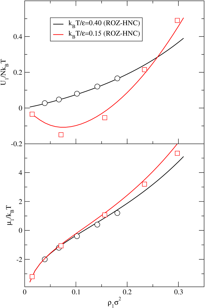
Figure 1: Average fluid excess internal energy and chemical potential for a matrix density $\rho_{0}\sigma^{2}=0.314$ at various temperatures.

In Figure 1 we plot the adsorption isotherms (lower curve) and the excess potential energy for a relatively high temperature ($k_{B}T/\varepsilon=0.4$) and a much lower one ($k_{B}T/\varepsilon=0.15$), for which clustering effects can be appreciated. Actually, the low density non-monotonous behavior of the internal energy reflects the competition between attractive forces (dominant at low densities) and repulsive forces that start to shape the system’s behavior for densities above $\rho_{1}\sigma^{2}\approx 0.06$. A signature of clustering can be appreciated in Figure 2 where the fluid-fluid structure factor, $S_{11}(q)$ calculated from the ROZ-HNC equation is compared with the one extracted from the simulation. This quantity is defined as

$$S_{11}(q)=1+\rho_{1}\tilde{h}_{11}(0)=\frac{1}{N_{1}}\left<|\sum_{i=1}^{N_{1}}e^{i{\bf q}{\bf r}_{i}}|^{2}\right>$$ (23)

where $N_{1}$ is the number of fluid particles and $<\ldots>$ denotes the ensemble average. In Eq. (23), the fluid-fluid correlation function must be replaced (in the ROZ formalism) by its connected counterpart, $h_{11}(r)-h_{11}^{r}(r)$, when the average over disorder is performed.

The simulation results presented in the Figure 2 correspond to a molecular dynamics (MD) run for a single matrix configuration and in which the initial fluid configuration is generated in a GCMC run. MD results correspond to averages carried out for one to two million configurations, using samples with 441 and 2399 fluid and matrix particles respectively and an integration time step of 0.0025 in reduced time units. The matrix density in this case is $\rho_{0}\sigma^{2}=0.324$, slightly above the one used in the solution of the ROZ-HNC equations. The presence of intermediate range orderGodfrin et al. (2013), which in our case can be identified with clustering, is indicated by the marked pre-peak in the fluid-fluid structure factor at $q=0.578\sigma^{-1}$, that reflects intercluster correlations for distances around $11\sigma$. For comparison in the lower graph we present results obtained using the same matrix and initial fluid configuration but with interactions of a LJ fluid, Eq. (5). We observe in the latter case that the structure factor lacks any signature of intermediate range order, but it clearly shows signs of an approaching divergence at $q\rightarrow 0$, i.e. the vicinity of the condensation transition.

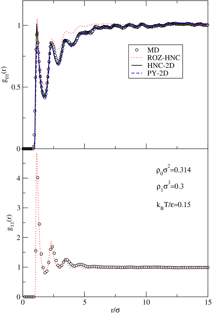
Figure 3: Average matrix-fluid and fluid-fluid correlations for a SALR fluid inclusion as estimated from MD simulations run from a given GCMC configuration with a fixed matrix configuration and by means of of PY-2D and HNC-2D equations and ROZ-HNC equations. Note that the ROZ equations provide the average of the correlations over matrix disorder.

In the lower graphs of Figures 3 and 4, we can see the performance of the ROZ-HNC equation for the calculation of the fluid-fluid correlations, which is relatively good for the high density case ($\rho_{1}\sigma=0.3$, cf. Fig. 3) and acceptable for the low density ($\rho_{1}\sigma=0.0596$, cf. Fig. 4). Differences can be in part attributed to the fact that we are comparing the ROZ results obtained for a matrix density $\rho_{0}\sigma^{2}=0.314$ with those of the simulation sample for which $\rho_{0}\sigma^{2}=0.324$, with the additional modification induced in the matrix topology by the removal of disconnected matrix particles. Notice that both theory and simulation reproduce the presence of a wide maximum at approximately $11\sigma$, in correspondence with the location of the pre-peak in $S_{11}(q)$. The comparison of the ROZ-HNC data with simulation results considerably worsens for the fluid-matrix correlations (upper graphs in the same figures), particularly at low density where clustering is more evident. Obviously, this discrepancy results from the poor description of matrix-matrix correlations when using $\rho_{0}\sigma^{2}=0.314$ ROZ results to model those of $\rho_{0}\sigma^{2}=0.324$, which is particularly crucial for the $g_{01}(r)$ correlations at low fluid densities. For higher fluid densities, the packing effects of the fluid dominate and this explains why the ROZ performance for $\rho_{1}\sigma^{2}=0.3$ is far better than for $\rho_{1}\sigma^{2}=0.0596$, as far as matrix-fluid correlations are concerned.

Nonetheless, we will only need the fluid-fluid correlations $g_{11}(r)$ to solve the HNC-2D equation (9), and those are reasonably approximated by the ROZ-HNC. The solution of the HNC-2D is done using a discretized two dimensional grid of $N_{x}\times N_{y}$ points (in this case $N_{x}=N_{y}=512$) with a grid spacing that is given by $\delta x=L_{x}/N_{x}$ and $\delta y=L_{y}/N_{y}$, where $L_{x}$ and $L_{y}$ represent the size of the simulation box corresponding to the matrix configuration whose fluid density distribution will be calculated using Eq. (9). Here, we will consider $L_{x}=L_{y}=86.066\sigma$ for low fluid density calculations , $\rho_{1}\sigma^{2}=0.0596$, (with $\rho_{0}\sigma^{2}=0.324$) and $L_{x}=L_{y}=39.84\sigma$, for the moderately high fluid density, $\rho_{1}\sigma^{2}=0.3$ (with $\rho_{0}\sigma^{2}=0.314$). The first results that come out from the solution of the HNC-2D equation are the matrix-fluid correlations that are depicted in the upper graphs of Figures 3 and 4. It is evident that the full 2D approach considerably improves upon the ROZ-HNC approximation for the average $g_{01}(r)$ distributions for a specific matrix configuration, in particular at low densities. For the highest density we include in the Figures results from the PY-2D approximation (11), which in this particular instance is more or less of the same quality as the HNC.

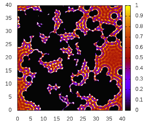
(a) MD

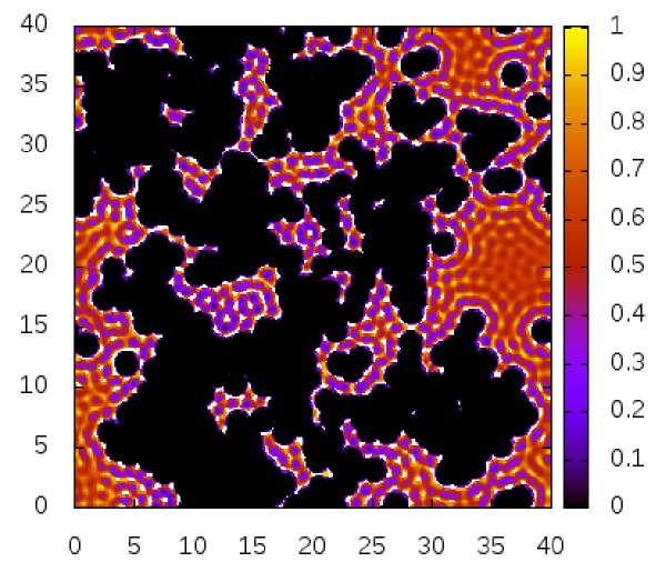
(b) HNC

Figure 5: Fluid density distribution $\rho_{1}(x,y)$ for the SALRC fluid for $\rho_{1}\sigma^{2}=0.3$ and $k_{B}T/\epsilon=0.15$ ($\rho_{0}\sigma^{2}=0.314$) from MD and in the HNC-2D approximation.

Now in Figures 5 and 6 we present the explicit 2D fluid density distributions $\rho_{1}(x,y)$, for $\rho_{1}\sigma^{2}=0.3$ ($\rho_{0}\sigma^{2}=0.314$), and $\rho_{1}\sigma^{2}=0.0596$ ($\rho_{0}\sigma^{2}=0.324$) for SALR fluids at temperatures where clustering becomes apparent (particularly at low density). One can immediately appreciate what we have commented upon above concerning the different matrix topologies. Despite the relatively small difference in the density $\rho_{0}$, one can see that the matrix porosity is appreciably larger for $\rho_{0}\sigma^{2}=0.324$ (Figure 6), and therefore matrix-matrix correlations (and hence matrix-fluid correlations as well) are quite different in both instances as we have seen. This effect is less appreciable in the fluid-fluid correlations, which are mostly conditioned by the effective density of the adsorbed fluid (similar in both cases).

In the case of the higher fluid density, in Figure 5 one readily observes that the HNC-2D equation actually reproduces quite well the simulated density distribution, and interestingly the maxima and minima of $\rho_{1}(x,y)$ are seen to display the features of a partly ordered system (approaching the local structure of a triangular lattice). Note that in this figure the black region represents the area of the system in which the fluid density vanishes. In this case this is precisely the area inaccessible to the centers of adsorbate atoms, i.e., the exclusion surface of the matrix as defined by the positions of its constituent atoms and their corresponding individuals exclusion surfaces. This exclusion surface per matrix particle is given for for our matrix-fluid interaction by $\approx\xi\pi\sigma^{2}$, with a parameter $\xi$ that accounts for the potential softness set to $\xi=0.98$ for the SALR potential, and $\xi=$0.8 for the LJ matrix-fluid interaction. In the case of the MD picture, the black region also includes those isolated matrix cavities that were empty from fluid particles in the starting configuration of the MD run. This empty cavities will be thus indistinguishable from the area of the sample excluded by the matrix in these spatial fluid density maps.

It can be appreciated that in the HNC-2D picture there is a substantially larger number of small disconnected pores partly filled with fluid inclusions as compared with the MD results. In this latter instance most of the disconnected pores happen to be empty for our particular initial fluid configuration. As mentioned, this results from the fact that our simulation corresponds to a MD run started from a single GCMC configuration of the fluid particles. A better agreement in this respect would be reached at a much higher computational cost calculating the fluid density $\rho_{1}(x,y)$ as the average from a series of MD runs started from different GCMC configurations of the fluids sampling the same chemical potential. In this case, the average population of the disconnected pores would be determined by the equilibrium grand canonical partition function and we would not have to rely on a single initial fluid configuration which might well be away from the equilibrium average. Notice that for large pores, the subsequent MD sampling would essentially converge toward the GCMC result. An alternative approach, would be the use of configurations in which fluid particles are not allowed to populate disconnected cavities in the matrix, and modify consequently the matrix-adsorbate interaction in the HNC-2D approach to include an artificial hard core potential that forces $\rho_{1}(x,y)\rightarrow 0$ inside these isolated cavities (e.g. retaining the template matrix particles that occupy these cavities in the original non-additive hard disk mixture). For simplicity, we have retained the original control pore glass like interaction and used our initial test GCMC results as input to generate the MD trajectories.

On the other hand, the reason for using MD generated configurations and not the output of the GCMC directly, is simply related to computational efficiency in the calculation of the simulated $\rho_{1}(x,y)$. In order to obtain a smooth density distribution, one needs to perform an intensive sampling of the configurational space with a large number of averages of spatially contiguous particle configurations, which is much simpler to attain using MD.

In Figure 6 we observe a density distribution $\rho_{1}(x,y)$ characteristic of the presence of clustering. One sees immediately that there are spatially separated regions of substantially higher fluid density, which tend to concentrate in pockets and bays of the porous structure, despite the fact that the matrix-fluid interaction is purely repulsive. This is due to the fact that, once particles aggregate in clusters as a consequence of the short range attractive part of the potential, the long-range repulsion between the clusters pushes them apart to places where at least some of them are “sheltered” by matrix particles. The intercluster separation lies in the range $10\sigma\sim 11\sigma$, in agreement with the position of the $S_{11}(q)$ pre-peak and the wide maximum of $g_{11}(r)$. The theoretical results are in excellent agreement with the simulated density distribution. Moreover, we have seen that as the simulation proceeds the results tend to approach to the theoretical prediction, since the reorganization of the clusters is a relatively slow process, particularly when they get trapped in narrow pockets. This is one of the reasons why the MD simulations have to be exceptionally long to yield a reliable $\rho_{1}(x,y)$. As an illustration, the fluid density inside the cavity at $\approx(12\sigma,55\sigma)$ in Figure 6(a) was found to remain well above $\rho_{1}(x,y)\sigma^{2}>0.3$ for close to one million MD steps, to slowly decrease and reach $\approx 0.17$ after another two million steps, much closer to the predicted HNC-2D estimate seen in Figure 6(b).

In order to appreciate the performance of the integral equations more quantitatively, in Figure 7 we plot the density profiles along the $x$-axis using as reference a given matrix particle. We observe that the PY-2D approximation underestimates the value of the density minima, and the HNC-2D slightly overestimates the maxima, which is a characteristic feature of the HNC correlation functions. Note that the theoretical profile exhibits some spikes corresponding to fluid particle inclusions in the aforementioned isolated cavities. These spikes are either absent in the MD results or have a much lower intensity, as a result of a much lower (or zero) initial density of fluid particles in the cavity in the starting MD configuration. This is again explained in the preceding paragraph as a result of the use of a single GCMC configuration as starting point for our MD calculations. Aside from this detail, the agreement between the theory and the simulation is remarkable.

Finally, for the sake of comparison we have run a long MD simulation (two million independent configurations in a run of ten million time steps) from the same starting fluid and matrix configuration as before ($\rho_{0}\sigma^{2}=0.324$), but where now fluid-fluid and matrix-fluid interactions are truncated and shifted LJ potential. The temperature of the run was set to $k_{B}T/\varepsilon=0.55$ and the fluid density as before $\rho_{1}\sigma^{2}=0.0596$. These conditions are quite close to the gas-liquid transition as can be inferred from the large $S_{11}(0)$ values in Figure 2. We have solved the ROZ-HNC equations for this system and obtained the density distribution using the HNC-2D equation. In Figure 8 we show the fluid-matrix and fluid-fluid correlations. As in the case of the low density SALR fluid, again here the fluid-matrix correlation ROZ-HNC predictions are rather poor, due to the inaccurate representation of the matrix-matrix correlations for this matrix configuration. Also, fluid-fluid correlations do not show any trace of intermediate long range ordering or clustering (the high values of the first peak of $g_{11}(r)$ are just an indication of confinement and the fluid-fluid correlation dies out rapidly). This is in clear contrast with the long range features found in Figure 4. Again, the HNC-2D fluid-matrix correlation agrees quite well with the MD results.

Now, the fluid density distribution for the same density as that of Figure 6 can be seen for the LJ system in Figure 9, and again we appreciate a remarkable agreement between theory and simulation. In this case, the simulation had to be particularly long for the density distribution to be smooth enough. The only salient feature appreciated in Figure 9 is the fact that the fluid density is enhanced near the pore walls, due to the attractive nature of the matrix particles. During the simulation run one can see the formation of short lived aggregates as a consequence of the vicinity of the liquid-gas transition, but in contrast to the SALR fluid, they have no preferred positions within the pore space, and the local density enhancements average out. Again, in Figure 10 we can have a more quantitative appreciation of the quality of the results in the density profile along the $x$-axis. The attractive nature of the pore particles is evidenced by the large values of $\rho_{1}(x,0)$ near the matrix particle boundaries, in contrast to the situation in Figure 7, where the repulsive nature of matrix-particle interaction used for the SALR fluid simulations is evident.

In summary, we have explored the ability of a full 2D solution of the HNC (and PY) equation for a fluid inclusion in a disordered porous matrix with a large degree of porosity. The equation was complemented by the use of a ROZ-HNC equation to faithfully approximate the fluid-fluid correlations under confinement. We have shown that this approach reproduces in a satisfactory way the average fluid-fluid spatial correlations of different types of adsorbates and its combination with the HNC-2D equation also yields a fair approximation for the matrix-fluid correlations. This avenue can be further exploited using the spatial decomposition approachYamazaki and Kovalenko (2011) to analyze the solvation free energy contribution in specific regions of the adsorbate, which can be of use when dealing with functionalized substrates. The application to three dimensional systems, mixtures and molecular adsorbates is currently work in progress.

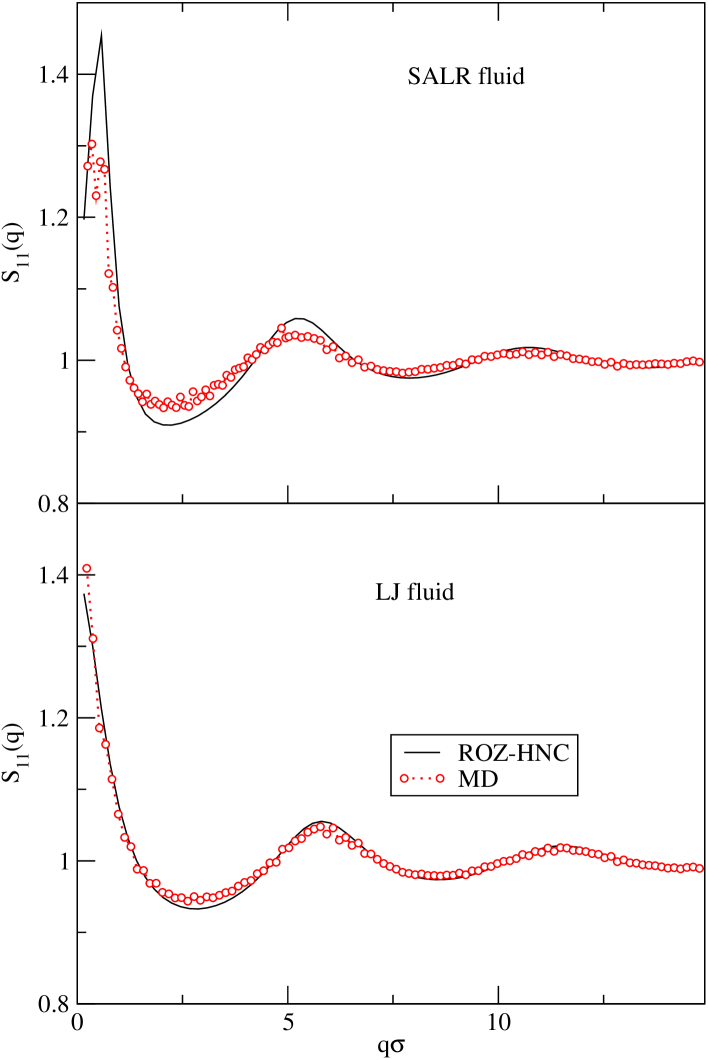
Figure 2: Fluid-fluid structure factor as calculated from the ROZ-HNC equation (curves) and from MD (symbols) for the adsorbed SALR fluid (upper graph) and the LJ system (lower graph) for $\rho_{1}\sigma^{2}=0.0596$ and $\rho_{0}\sigma^{2}=0.324$. Note the marked pre-peak at $q=0.578\sigma$ for the SALR fluid. The LJ fluid $S_{11}(q)$ grows as $q\rightarrow 0$, which indicates the vicinity of the condensation transition.

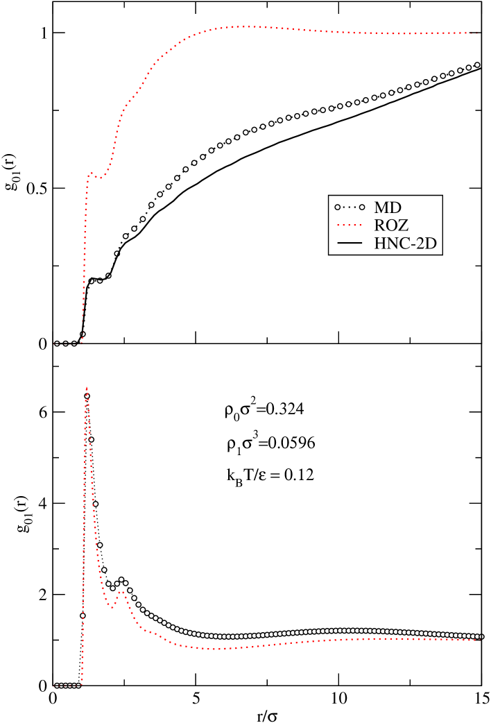
Figure 4: Same as figure 3 for a much lower fluid density for which clustering effects are more apparent, as can be inferred by the long range of the fluid-fluid correlations, $g_{11}(r)$, which exhibit a wide maximum around $11\sigma$.

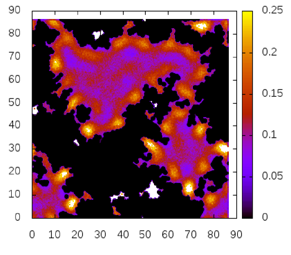
(a) MD

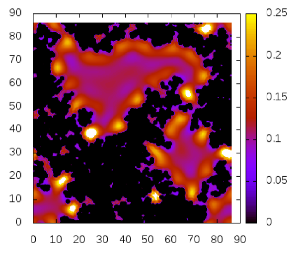
(b) HNC

Figure 6: Fluid density distribution $\rho_{1}(x,y)$ of the SALR fluid for $\rho_{1}\sigma^{2}=0.0596$ and $k_{B}T/\epsilon=0.12$ ($\rho_{0}\sigma^{2}=0.324$) from MD and in the HNC-2D approximation. Regions for which $\rho_{1}(x,y)>0.25$ are plotted in white.

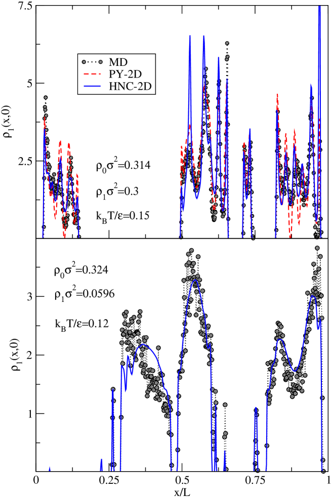
Figure 7: Illustration of the density profile $\rho_{1}(x,0)$ of the SALR fluid along the $x$-axis taking as origin a given matrix particle. The upper figure corresponds to the density map of Figure 5 and the lower one to the map of Figure 6. Distances are scaled with the side of the simulation box since each figure corresponds to samples of different size, and the reference matrix particle is also a different one.

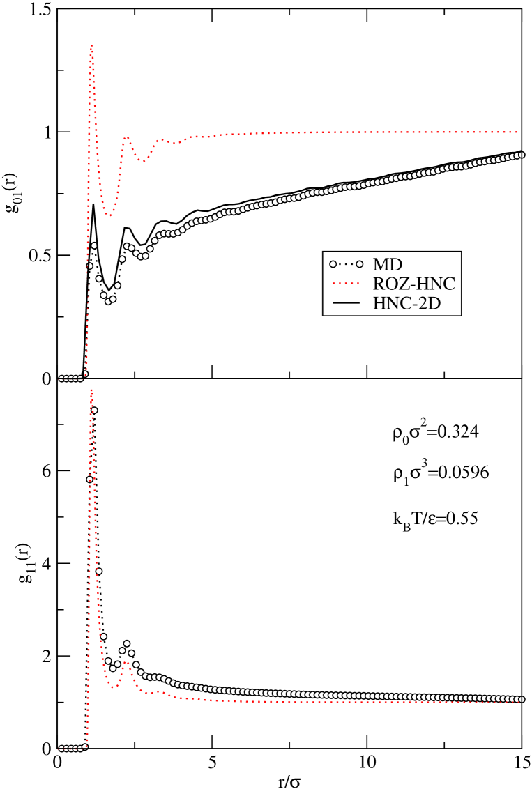
Figure 8: Same as figure 4 for a LJ fluid in a LJ matrix. Note the higher intensity of the first peaks as a consequence of the LJ attraction, the pronounced spatial structure of $g_{01}(r)$ and the lack of maximum at $10\sigma$ in $g_{11}(r)$ due to the absence of clustering.

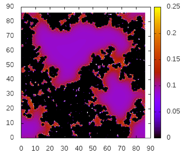
(a) MD

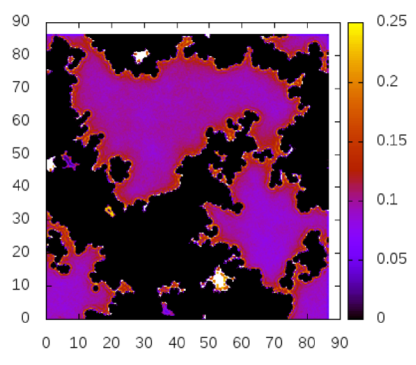
(b) HNC

Figure 9: Fluid density distribution $\rho_{1}(x,y)$ for $\rho_{1}\sigma^{2}=0.0596$ and $k_{B}T/\epsilon=0.55$ ($\rho_{0}\sigma^{2}=0.324$) from MD and in the HNC-2D approximation for a LJ fluid inclusion in a matrix formed by LJ particles.

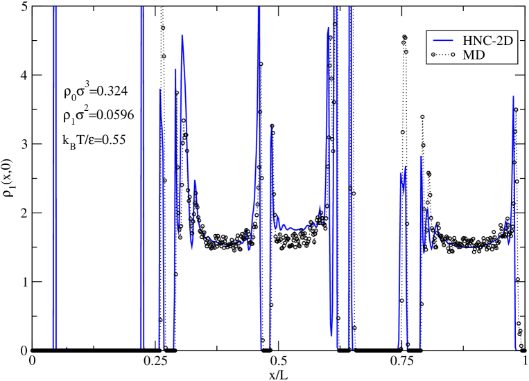
Figure 10: Illustration of the LJ fluid density profile $\rho_{1}(x,0)$ along the $x$-axis taking as origin a given matrix particle. The fluid-matrix attraction is reflected in the large values of the density profile in the immediate vicinity of the matrix particles.