Implementation of Lévy CARMA model in Yuima package

Abstract

The paper shows how to use the R package yuima available on CRAN for the simulation and the estimation of a general Lévy Continuous Autoregressive Moving Average (CARMA) model. The flexibility of the package is due to the fact that the user is allowed to choose several parametric Lévy distribution for the increments. Some numerical examples are given in order to explain the main classes and the corresponding methods implemented in yuima package for the CARMA model.

1 Introduction

The Continuous Autoregressive Moving Average (CARMA) model driven by a standard Brownian Motion was first introduced in the literature by [17] as a continuous counterpart of the discrete-time ARMA process and, recently, it has gained a rapid development in theory and practice. Indeed, in order to increase the level of appealing in different areas, the gaussianity assumption is relaxed and a CARMA model driven by a Lévy process with finite second order moments has been introduced in [9]. In this way the marginal distribution of the CARMA process is allowed to be asymmetric and heavy-tailed. For this reason the CARMA model is widely applied in the financial literature.
For example, [2] used a Lévy CAR(1) (or Ornstein Uhlenbeck) process for building a stochastic volatility model while [28] and [27] applied the Lévy CARMA(2,1) for modeling the volatility of the Deutsche Mark/US Dollar daily exchange rate. Moreover [10] proposed the fractionally integrated CARMA model in order to capture the long range dependence usually observed in financial time series.

The interest on the CARMA model is manifold since it can be used to model directly some given time series but it is also a main block for the construction of a more general process like the COGARCH(p,q) as in [5].

The aim of this work is to develop in the yuima package a complete computational scheme for the simulation and the estimation of a general Lévy CARMA model. Based on our knowledge, the R packages available on CRAN deal only with CARMA(p,q) models driven by a standard Brownian Motion [30] or Gaussian CAR(p) models [33].
For example the ctarma package developed by [29] is an useful package for the simulation and the estimation of a CARMA(p,q) model driven by a Brownian Motion. Another package for continuous Autoregressive model is the cts developed by [33] which deals with a modified version of the CAR(p) model named CZAR(p) by [32].
Since the CAR(p) model is a special case of a CARMA(p,q), the ctarma package is a valid benchmark for the functions implemented in the yuima package and for this reason a direct comparison is given in this paper where a Gaussian CARMA(p,q) model is considered. Moreover, in the yuima package, once the estimation of the coefficients is done, it is possible to recover the underlying Lévy process from the observed data using the methodology in [7] and extended to the multivariate CARMA(p,q) by [8]. In this way we are able to simulate trajectories of a CARMA model without an explicit assumption on the distribution at time one of the underlying Lévy process.
The outline of this paper is the following. In Sect. 2 we review the main results about the CARMA(p,q) process. In particular we focus the attention on the condition for the existence of the second order stationary solution of the CARMA process. In Sect. 3 we explain the estimation procedure implemented in the yuima package if the data are observed in equally space-time intervals. In Sect. 4 we describe the main classes and corresponding methods available in the yuima package for a CARMA model. We show how to use them for simulation and estimation of a Gaussian CARMA model and we conduct a comparison with the methods availables in the ctarma package. In Sect. 5 we present some numerical examples about the simulation and the estimation of Lévy CARMA models.

2 Continuous ARMA Models driven by a Lévy process

In this section we review the main features of a CARMA(p,q) model driven by a Lévy process introduced in [9]

Definition 1

Let $p,\ q$ non-negative integers such that $p>q\geq 0$. The CARMA(p,q) process is defined as:

$$a(D)Y_{t}=b(D)DL_{t}$$ (1)

$D$ is the differentation operator with respect to $t$ while $a\left(\cdot\right)$ and $b\left(\cdot\right)$ are two polynomials:

$$a\left(z\right)=z^{p}+a_{1}z^{p-1}+\cdots+a_{p}$$

$$b\left(z\right)=b_{0}+b_{1}z^{1}+\cdots+b_{p-1}z^{p-1}$$

where $a_{1};\cdots;a_{p}$ and $b_{0},\cdots,b_{p-1}$ are coefficients such that $b_{q}\neq 0$ and $b_{j}=0$ $\forall j>q$.

Since the higher order derivatives of a Lévy process are not well defined we use the state space representation of a CARMA(p,q) model.

$$Y_{t}=\mathbf{b}^{\intercal}X_{t}$$ (2)

where $X_{t}$ is a vector process of dimension $p$ satisfying the following system of stochastic differential equations:

$$\mbox{d}X_{t}=AX_{t}\mbox{d}t+\mathbf{e}\mbox{d}L_{t}$$ (3)

where the $p\times p$ matrix $A$ is defined as:

$$A\ =\ \left[\begin{array}[]{ccccc}0&1&0&\ldots&0\\ 0&0&1&\ldots&0\\ \vdots&\vdots&\vdots&\ldots&\vdots\\ 0&0&0&\ldots&1\\ -a_{p}&-a_{p-1}&-a_{p-2}&\ldots&-a_{1}\\ \end{array}\right]$$

The $p\times 1$ vectors $\mathbf{e}$ and $\mathbf{b}$ are respectively:

$$\mathbf{e}=\left[0,\ldots,0,1\right]^{\intercal}$$

$$\mathbf{b}=\left[b_{0},\ldots,b_{p-1}\right]^{\intercal}.$$

Given the initial condition on $X_{s}$, the solution of equation (3) is:

$$X_{t}=e^{A\left(t-s\right)}X_{s}+\int_{s}^{t}e^{A\left(t-u\right)}\mathbf{e}\mbox{d}L_{u},\ \ \forall t>s.$$ (4)

Where the matrix exponential $e^{A}$ is defined as a power series:

$$e^{A}=\sum_{h=0}^{+\infty}\frac{1}{h!}A^{k}.$$

The following result, given in [9], provides the necessary and sufficient conditions for the existence of a stationary solution $X_{t}$ of system (3) such that $X_{t}$ is independent of $\left\{L_{h}-L_{s},\ h>s\right\}\ \forall t\in R$

Proposition 2

The process $X_{t}$ of system (3) has a covariance stationary solution if and only if the real part of the eigenvalues $\lambda_{1},\ \dots,\ \lambda_{p}$ of matrix $A$ are negative, i.e.

$$\operatorname{Re}\left(\lambda_{i}\right)<0,\ \ i=1,\ \dots,\ p.$$

The solution can be written as:

$$X_{t}=\int_{-\infty}^{t}e^{A\left(t-u\right)}\mathbf{e}\mbox{d}L_{u}\buildrel d\over{=}\int_{0}^{+\infty}e^{Au}\mathbf{e}\mbox{d}L_{u}$$ (5)

and the associated first and second moments are:

$$E\left[X_{t}\right]=\frac{\mu}{a_{p}}\mathbf{e}$$

$$Cov\left[X_{t+h};X_{t}\right]=\sigma^{2}e^{Ah}\int^{+\infty}_{0}e^{Au}\mathbf{e}\mathbf{e}^{\intercal}e^{A^{\intercal}u}\mbox{d}u\ \ for\ \ h\geq 0.$$

where $\mu=E\left[L_{1}\right]$ and $\sigma^{2}=Var\left[L_{1}\right]$

Remark 3

We observe that matrix $A$ can be diagonalized as follows:

$$A=R\Lambda R^{-1}.$$

$\Lambda$ is a matrix whose elements along the diagonal are the eigenvalues of $A$ and the other elements are zero.

$$\Lambda=diag(\lambda_{j})\ \ \ j=1,\ldots,p.$$

The columns of $R$ are the eigenvectors of $A$ which are obtained easily from the eigenvalues:

$$R_{,j}=\left[1,\lambda_{j},\lambda^{2}_{j},\ldots,\lambda_{j}^{p-1}\right]^{\intercal},\ \ \ j=1,\ldots,p.$$

The necessary and sufficient condition for the diagonalization of $A$ is that the eigenvalues $\lambda_{j},\ \ \ j=1,\ldots,p$ are distincts.

Using equation (5), the solution of CARMA process $Y_{t}$ has the following form:

$$Y_{t}=\mathbf{b}^{\intercal}X_{t}=\int_{-\infty}^{+\infty}g\left(t-u\right)\mbox{d}L_{u}.$$

where $g\left(t\right)=\mathbf{b}^{\intercal}e^{At}\mathbf{e}\mathbbm{1}_{\{\left[0,+\infty\right)\}}\left(t\right)$ is the Kernel of the CARMA process $\left\{Y_{t}\right\}$ and $\mathbbm{1}_{\{A\}}\left(x\right)$ is the indicator function defined as:

$$\mathbbm{1}_{\{A\}}\left(x\right):=\left\{\begin{array}[]{lll}1&&x\in A\\ 0&&x\notin A\\ \end{array}\right.$$

.

Proposition 4

Under the assumptions that the eigenvalues of matrix $A$ are distinct and $\operatorname{Re}\left(\lambda_{i}\right)<0$ for $i=1,\ldots,p.$ the CARMA(p,q) process can be obtained as a sum of dependent CAR(1) processes:

$$Y_{t}=\sum_{r=1}^{p}Y_{r,t}$$ (6)

where

$$Y_{r,t}=\int_{-\infty}^{t}\alpha_{r}e^{\lambda_{r}\left(t-u\right)}\mbox{d}L_{u},$$ (7)

$$\alpha_{r}=\frac{b\left(\lambda_{r}\right)}{a^{\prime}\left(\lambda_{r}\right)},\ \ \ r=1,\ldots,p.$$ (8)

and $a^{\prime}(z)$ is the first derivative of the polynomial $a\left(z\right)$.

In particular, the vector $\tilde{Y_{t}}=\left[Y_{1,t},\ldots,Y_{p,t}\right]$, whose elements are the CAR(1) processes necessary in the representation (6), can be obtained as:

$$\tilde{Y}_{t}=\tilde{\Lambda}R^{-1}X_{t}$$ (9)

Where $\tilde{\Lambda}$ is a diagonal matrix defined as:

$$\tilde{\Lambda}=\operatorname{diag}\left[b\left(\lambda_{i}\right)\right]_{i=1}^{p}.$$

This is the canonical representation of CARMA process, the vector $\tilde{Y_{t}}$ is the canonical state vector and it will be useful for recovering the increments of the underlying noise.

3 Estimation of a CARMA(p,q) model in the yuima package

In this Section we discuss the estimation procedure implemented in the yuima package for a CARMA model driven by a Lévy process. From now on, we assume that the condition for canonical state representation (i.e. distinct eigenvalues for $A$ matrix whose real part is negative) is satisfied. As observed before, we consider a three step procedure:

1. Exploiting the state space representation, we estimate the CARMA parameters $\mathbf{a}:=\left[a_{1},\ldots,a_{p}\right]$ and $\mathbf{b}:=\left[b_{0},\ldots,b_{q},b_{q+1}=0,\ldots,b_{p-1}=0\right]$ through the quasi-maximum likelihood estimation (see [25] for univariate and multivariate cases). An alternative approach is based on the Least Square estimation (see [7] for more details).Since the state space representation in system (3) is based on the unbservable process $X_{t}$, we implement a Kalman Filter procedure (see [29] for a CARMA model driven by a brownian motion).

2. Once the CARMA parameters have been found, we recover the increments of the underlying Lévy following the approach proposed in [7] as a generalization of the approach developed in [6] for the continuous autoregressive process. Recently the same approach has been applied to the multivariate case by [8].

3. In the last step, using the increments estimated in the previous step, we estimate the parameters of the Lévy measure. The likelihood function is computed by means of the Fourier Transform for all Lévy increments assumption available in the yuima package.

Following [7] we assume that the observations $Y_{1},\ldots,Y_{n},\ldots,Y_{T}$ are collected at equally spaced time instants $0,h,2h,\dots,Nh$ where $N$ is the number of obsevations and $h$ is the step length. In this context, the time horizon $T$ is equal to $Nh$.
In order to be more general as possible, the expectation and the variance of the Lévy at time 1 are given by:

$$E\left[L_{1}\right]=\mu\ \ \ Var\left[L_{1}\right]=\sigma^{2}.$$

Then we define a mean corrected process $Y^{\star}_{n}$ as:

$$Y^{\star}_{n}=Y_{n}-E\left[Y_{n}\right].$$ (10)

Let $Y_{n}$ be a ergodic series, we estimate the expectation in (10) using the sample mean. Finally, the process $Y^{\star}_{n}$ has again a state space representation:

$$Y^{\star}_{n} = \mathbf{b}^{\intercal}X^{\star}_{n}$$

$$X^{\star}_{n} = e^{Ah}X^{\star}_{n}+U_{n}$$

Where $X^{\star}_{n}$ is a sample mean corrected state vector process of the $X_{t}$ in system (3). $e^{A}$ is the matrix exponential of $A$. $U_{n}$ is a sequence of i.i.d random vectors with zero mean and variance-covariance matrix:

$$Q=\int_{0}^{h}e^{Au}\mathbf{e}\mathbf{e}^{\intercal}e^{A^{\intercal}u}\mbox{d}u$$ (11)

Remark 5

If $Y_{t}$ is a CARMA process driven by a Brownian Motion then the sampled process $Y_{n}$ is a Gaussian ARMA process with i.i.d. noise for any step length $h$. For a second order Lévy CARMA process, the driving noise is not necessarly i.i.d. but the sampled process $Y_{n}$ is still an ARMA process. In this case the process $Y^{\star}_{n}$ is a weak ARMA process and the distribution of the maximum likelihood estimators can be derived using the result in [18].

Before introducing the Kalman Filter algorithm (see [20] for more details) we need to compute the $Q$ matrix in (11). We start by evaluating the stationary unconditional variance-covariance matrix $Q_{\infty}$ satisfying the system of equations (see [31] for more details):

$$AQ_{\infty}+Q_{\infty}A^{\intercal}=-\sigma^{2}\mathbf{e}\mathbf{e}^{\intercal}$$

then the matrix $Q$ is obtained using the following formula:

$$Q=Q_{\infty}-e^{Au}Q_{\infty}e^{A^{\intercal}u}$$

Using this result, the Kalman Filter algorithm gives us a simple and analytical way for computing the likelihood function. The estimation procedure based on the Kalman Filter can be summarized into four steps: initialization, prediction, correction and construction of the log-likelihood function.
Before explaining the steps in the Kalman Filter algorithm we need to clarify the used notations. We define $X^{\star}_{n\left|n-1\right.}$ and $\Sigma_{n\left|n-1\right.}$ the prior estimates of the state variables process and the Variance-Covariance matrix of the error term $U_{n}$, i.e.

$$X^{\star}_{n\left|n-1\right.} = E\left[X^{\star}_{n}\right|\left.I_{n-1}\right]$$

$$\Sigma_{n\left|n-1\right.} = Var\left[U_{n}\right|\left.I_{n-1}\right]$$

where the $\sigma-$algebra $I_{n-1}$ is generated by the observations of the process $Y^{\star}_{n}$ and by the estimates of the state space variables up to time $n$:

$$I_{n-1}=\sigma\left(Y^{\star}_{n-1},\ldots,Y^{\star}_{0},X^{\star}_{n-1\left|n-1\right.},\ldots,X^{\star}_{0\left|0\right.}\right).$$

We denote with $X^{\star}_{n\left|n\right.}$ and $\Sigma_{n\left|n\right.}$ the posterior estimates for the mean corrected state process $X^{\star}$ and the Variance-Covariance matrix for the process $U_{n}$. In this case the estimates are obtained according to the augmented $\sigma-$algebra $I^{\star}_{n}$:

$$I^{\star}_{n}=\sigma\left(\left\{I_{n-1}\right\}\cup\left\{Y^{\star}_{n},X^{\star}_{n\left|n-1\right.}\right\}\right).$$

Initialization.
We initialize the state variable $X^{\star}_{n}$ at zero since, under the assumption that the eigenvalues of Matrix $A$ are distinct with negative real part, the unconditional mean $E\left[X^{\star}_{n}\right]$ is equal to zero while the variance-covariance matrix is initialized at the uncoditional variance-covariance matrix $Q_{\infty}$. Finaly we set:

$$X^{\star}_{0\left|0\right.} = 0=X^{\star}_{n-1\left|n-1\right.}$$

$$\Sigma_{0\left|0\right.} = Q_{\infty}=\Sigma_{n-1\left|n-1\right.}$$

Prediction.
We start by predicting the unobservable process $X^{\star}_{n\left|n-1\right.}$ and the variance-covariance matrix $\Sigma_{n\left|n-1\right.}$

$$X^{\star}_{n\left|n-1\right.} = e^{Ah}X^{\star}_{n-1\left|n-1\right.}$$

$$\Sigma_{n\left|n-1\right.} = e^{Ah}\Sigma_{n-1\left|n-1\right.}e^{A^{\intercal}h}+Q$$

then we can forecast the observable process $Y_{n}$:

$$Y^{\star}_{n\left|n-1\right.}=b^{\intercal}X^{\star}_{n\left|n-1\right.}.$$

We define the error term $u_{n}$ as:

$$u_{n}=Y^{\star}_{n}-b^{\intercal}X^{\star}_{n\left|n-1\right.}$$

where $Y^{\star}_{n}$ is the observed mean corrected process defined in (10). Thus, the error term $u_{n}$ is normally distributed

$$u_{n}\sim N\left[0,\ \mathbf{b}^{\intercal}\Sigma_{n\left|n-1\right.}\mathbf{b}\right]$$

and we use the result to build the log-likelihood function.
Correction
We need to update the state variable $X^{\star}$ and the variance-covariance matrix $\Sigma$ since we observe the realization of the process $Y^{\star}_{n}$.

$$X^{\star}_{n\left|n\right.} = X^{\star}_{n\left|n-1\right.}+K_{n}\left(Y^{\star}_{n}-Y^{\star}_{n\left|n-1\right.}\right)$$

$$\Sigma_{n\left|n\right.} = \Sigma_{n\left|n-1\right.}-K_{n}\mathbf{b}^{\intercal}\Sigma_{n\left|n-1\right.}$$

where $K_{n}$ is the Kalman Gain Matrix and it is defined as:

$$K_{n}=\Sigma_{n\left|n-1\right.}\mathbf{b}\left(\mathbf{b}^{\intercal}\Sigma_{n\left|n-1\right.}\mathbf{b}\right)^{-1}.$$

We use the updated state variable $X_{n\left|n\right.}$ and the variance-covariance matrix $\Sigma_{n\left|n\right.}$ as inputs in (LABEL:init-step) and we repeat steps $1\div 3$ until $n=N$.
Construction of the log-likelihood function
Once all error terms $\left\{u_{n}\right\}_{n=1}^{N}$ are obtained, we compute the log-likelihood function:

$$\mathscr{L}\left(\mathbf{a},\mathbf{b}\right)=-\frac{1}{2}\sum_{n=1}^{N}\ln\left(2\pi\mathbf{b}^{\intercal}\Sigma_{n\left|n-1\right.}\mathbf{b}\right)-\frac{1}{2}\sum_{n=1}^{N}\frac{u_{n}^{2}}{\mathbf{b}^{\intercal}\Sigma_{n\left|n-1\right.}\mathbf{b}}$$ (13)

and get the estimates for vectors $\mathbf{a}$ and $\mathbf{b}$ by maximizing the quantity in (13). In the yuima package constrained optimization is also available.
Once the estimates for vectors $\mathbf{a}$ and $\mathbf{b}$ are obtained, the next step is to retrieve the increments of underlying Lévy process. It is worth to notice that the procedure for recovering the underlying Lévy increments is a non-parametric approach since the knowledge of the distribution is not necessary at this stage while it becomes relevant in the last passage of the estimation procedure implemented in yuima package.
Following [7], the vector $\tilde{X}_{q,t}$ composed by the firsts $q-1$ components of the state process $X_{t}$ in (4), can be written in terms of the observable process $Y_{t}$.

$$\mbox{d}\tilde{X}_{q,t}=B\tilde{X}_{q,t}\mbox{d}t+\mathbf{e_{q}}Y_{t}\mbox{d}t$$ (14)

where the matrix $B$ is defined as:

$$B\ =\ \left[\begin{array}[]{ccccc}0&1&0&\ldots&0\\ 0&0&1&\ldots&0\\ \vdots&\vdots&\vdots&\ldots&\vdots\\ 0&0&0&\ldots&1\\ -b_{0}&-b_{1}&-b_{2}&\ldots&-b_{q-1}\\ \end{array}\right]$$

and the vector $\mathbf{e_{q}}$

$$\mathbf{e_{q}}=\left[0,\ldots,0,1\right]^{\intercal}$$

The system of equations (14) has the explicit solution:

$$\tilde{X}_{q,t}=e^{Bt}\tilde{X}_{q,0}+\int_{0}^{t}e^{B\left(t-u\right)}\mathbf{e_{q}}Y_{u}\mbox{d}u$$

The remaining $p-q$ components of $X_{t}$ are obtained by computing the higher order derivatives of the first component $X_{0,t}$ of the state vector $X_{t}$ with respect to time:

$$X_{j,t}=\frac{\partial^{j-1}X_{0,t}}{\left(\partial t\right)^{j-1}},\ \ \ j=q,\dots,p-1.$$ (15)

Using the canonical form of a CARMA process in (9), we obtain the canonical state vector $\tilde{Y_{t}}$ and, following [6], the underlying Lévy can be expressed using one of the equation in the following system:

$$L_{t}=\frac{1}{\alpha_{r}}\left[\tilde{Y_{r,t}}-\tilde{Y_{r,0}}-\lambda_{r}\int_{0}^{t}Y_{r,u}\mbox{d}u\right]\ \ \ r=1,\ldots,p.$$ (16)

where $\alpha_{r}$ is defined in equation (8) and $\lambda_{r}$ is the rth eigenvalue of the matrix $A$. For estimation of the Lévy, as suggested in [7], we choose the condition in (16) such that the corresponding $\lambda_{r}$ is the largest real eigenvalue.
Once the increments of the underlying Lévy are obtained, in the yuima package, it is possible to estimate the parameters of the Lévy measure. We refer to the yuima documentation (see [26] for more details for the available Lévy processes in yuima package. The estimation procedure in this phase is the maximum likelihood and the density is obtained by inverse Fourier Transform.

4 Implementation of a CARMA(p,q) in the Yuima package

This Section is devoted to the description of the objects and methods available in the yuima package for defining a general CARMA model driven by a Lévy process in the R statistical environment [15].

The yuima package [26] is a comprehensive framework based on the S4 system of classes and methods (see [13] for a complete treatement of the S4 class system) which allows a description of stochastic differential equations with the following form:

$$\mbox{d}X_{t}=b\left(t,X_{t}\right)\mbox{d}t+\sigma\left(t,X_{t}\right)\mbox{d}W^{H}_{t}+c\left(t,X_{t}\right)\mbox{d}Z_{t}.$$

where $b\left(t,X_{t}\right)$, $\sigma\left(t,X_{t}\right)$ and $c\left(t,X_{t}\right)$ are coefficients defined by the user. $W^{H}_{t}$ is a fractional Brownian motion and $H$ is the Hurst index which default value is fixed to $\frac{1}{2}$ corresponding to the case of the standard Brownian motion (see [12] for estimation of $H$ index in yuima package) and $Z_{t}$ is a pure Lévy jump process (see [4, 24] for more details).

In this context, the mathematical description of a CARMA(p,q) process is done by the yuima constructor function setCarma that returns an object of class yuima.carma. Since the yuima.carma-class extends the yuima.model-class (see [11] for a complete description of an object of class yuima.model), it is possible to generate a sample path using the simulate method, estimate the parameters applying the qmle method and it is also available the utility toLatex that produce a LaTeXcode that returns the state space representation of the CARMA(p,q) model using the matrix notations. The method CarmaNoise works only for object of class yuima.carma and allows to retrieve the increments of the underlying Lévy following the approach described in Sect. 3 once the vectors $\mathbf{a}$ and $\mathbf{b}$ are known.

4.1 The yuima.carma-class

An object of the class yuima.carma contains all informations related to a general linear state space model that encompasses the CARMA model illustrated in Sect. 2.
The mathematical description of this general model is given by the following system of equations:

$$Y_{t} = c_{0}+\sigma\left(\mathbf{b}^{\intercal}X_{t}\right)$$

$$\mbox{d}X_{t} = AX_{t}\mbox{d}t+\mathbf{e}\left(\gamma_{0}+\gamma^{\intercal}X_{t}\right)\mbox{d}Z_{t}$$

where $c_{0}\in\mathcal{R}$ and $\sigma\in\left(0,+\infty\right)$ are location and scale parameters respectively. The vector $\mathbf{b}\in\mathcal{R}^{p}$ contains the moving average parameters $b_{0},b_{1},\ldots,b_{q}$ while the $A$ is a $p\times p$ matrix whose last row contains the autoregressive parameters $a_{1},\ldots,a_{p}$ and, as shown in Sect. 2. It is defined as:

$$A\ =\ \left[\begin{array}[]{ccccc}0&1&0&\ldots&0\\ 0&0&1&\ldots&0\\ \vdots&\vdots&\vdots&\ldots&\vdots\\ 0&0&0&\ldots&1\\ -a_{p}&-a_{p-1}&-a_{p-2}&\ldots&-a_{1}\\ \end{array}\right].$$

The $\gamma_{0}\in\mathcal{R}$ and the vector $\gamma:=\left[\gamma_{1},\ldots\gamma_{p}\right]$ are called linear parameters. The linear parameters $\left[\gamma_{0},\gamma_{1},\ldots\gamma_{p}\right]$ will play a central role for defining the COGARCH(p,q) model introduced in [5] in the yuima package that will be one of the main objects of future developements.
As noted previously, the yuima.carma extends the yuima.models and all features in this class are inherited. In particular the structure of an object of class yuima.carma is composed by the slots listed below:

• info is an object of carma.info-class that describes the structure of the CARMA(p,q) model.

• drift is an R expression which specifies the drift coefficient (a vector).

• diffusion is an R expression which specifies the diffusion coefficient (a matrix).

• hurst is the Hurst parameter of the fractional Brownian motion. The default value $\frac{1}{2}$ corresponds of the standard Brownian process.

• jump.coeff is a vector of expressions for the jump component.

• measure indicates the measure of the Lévy process.

• measure.type is a switch variable that indicates if the type of Lévy measure specified in the slot measure belongs to the class of Compound Poisson processes.

• state.variable indicates a vector of names identifying the names used to denote the state variable in the drift and diffusion specifications.

• parameter is a short name for “parameters”, is an object of class model.parameter-class. For more details see yuima documentation.

• state.variable identifies the state variables in the R expression.

• jump.variable identifies the variable for the jump coefficient.

• time.variableis the name of the time variable.

• noise.number denotes the number of sources of noise. Currently only for the Gaussian part.

• equation.number is the dimension of the stochastic differential equation.

• dimension is the dimension of the parameter given in the slot parameter.

• solve.variable identifies the variable with respect to which the stochastic differential equation has to be solved.

• xinit contains R expressions that are the initial conditions for the stochastic differential equations.

• J.flag is for internal use only.

It is worth to remark that, except for the slot info, the remainings are members of the yuima.model-class. Indeed the object of class carma.info in the slot info contains all informations about the CARMA model. It cannot be directly specified by the user but it is constructed by setCarma function that fills the following slots:

• p is a integer number the indicates the dimension of autoregressive coefficients.

• q is the dimension of moving average coefficients.

• loc.par is the label of location coefficient.

• scale.par indicates the Label of scale coefficient.

• ar.par denotes the label of autoregressive coefficients.

• ma.par is the label of moving average coefficients.

• lin.par indicates the label of linear coefficients.

• Carma.var denotes the label of the observed process.

• Latent.var is the label of the state process.

• XinExpr is a logical variable. If XinExpr=FALSE, the starting condition of Latent.var is zero otherwise each component of Latent.var has a parameter as a starting point.

4.2 CARMA model specification

In this section we explain how to use the constructor setCarma in order to build an object of class yuima.carma and we show how to simulate a trajectory of the CARMA(p,q) process using the same procedure available for an object of class yuima.model.
The arguments used in a call to the constructor setCarma() are:

setCarma(p,q,loc.par=NULL,scale.par=NULL,ar.par="a",ma.par="b",lin.par=NULL,
  Carma.var="v",Latent.var="x",XinExpr=FALSE, ...)

In the following we illustrate the arguments of the setCarma function:

• p is a non-negative integer that indicates the number of the autoregressive coefficients.

• q is a non-negative integer that indicates the order of the moving average coefficients.

• loc.par is a string for the label of the location coefficient. The default value loc.par=NULL implies that $c_{0}=0$.

• scale.par is a character-string that is the label of scale coefficient. The default value scale.par=NULL implies that sigma=1.

• ar.par is a character-string that is the label of the autoregressive coefficients. The default Value is ar.par="a".

• ma.par is a character-string specifying the label of the moving average coefficients. The default Value is ma.par="b".

• Carma.var is a character-string that is the label of the observed process. Defaults to "v".

• Latent.var is a character-string representing the label of the unobserved process. Defaults to "x".

• lin.par is a character-string that is the label of the linear coefficients. If lin.par=NULL, the default, the setCarma builds the CARMA(p,q) model defined as in [9].

• XinExpr is a logical variable. The default value XinExpr=FALSE implies that the starting condition for Latent.var is zero. If XinExpr=TRUE, each component of Latent.var has a parameter as a initial value.

• ... Arguments to be passed to setCarma, such as the slots of yuima.model-class. They play a fondamental role when the underlying noise is a pure jump Lévy process. In particular the following two arguments are necessary:

  • measure Lévy measure of jump variables.

  • measure.type type specification for Levy measure.

Assume that we want to build a CARMA(p=3,q=1) model driven by a standard Brownian Motion with location parameter. In this case, the state space model in (LABEL:gen-state-space-mod) can be written in a explicit way as follows:

$$Y_{t} = b_{0}X_{0,t}+b_{1}X_{1,t}$$

$$\mbox{d}X_{0,t} = X_{1,t}\mbox{d}t$$

$$\mbox{d}X_{1,t} = X_{2,t}\mbox{d}t$$

$$\mbox{d}X_{2,t} = \left[-a_{3}X_{0,t}-a_{2}X_{1,t}-a_{1}X_{0,t}\right]\mbox{d}t+dZ_{t}$$

where $Z_{t}$ is a Wiener process.
For this reason, we instruct yuima to create an object of class yuima.carma using the code listed below.

> Carma_brown_mod<-setCarma(p=3,q=1,loc.par="c0",Carma.var="y",Latent.var="X")

We can display the internal structure of the object Carma_brown_mod using the R utility str:

> str(Carma_brown_mod)

Formal class ’yuima.carma’ [package "yuima"] with 17 slots
  ..@ info           :Formal class ’carma.info’ [package "yuima"] with 10 slots
  .. .. ..@ p         : num 3
  .. .. ..@ q         : num 1
  .. .. ..@ loc.par   : chr "c0"
  .. .. ..@ scale.par : chr(0)
  .. .. ..@ ar.par    : chr "a"
  .. .. ..@ ma.par    : chr "b"
  .. .. ..@ lin.par   : chr(0)
  .. .. ..@ Carma.var : chr "y"
  .. .. ..@ Latent.var: chr "X"
  .. .. ..@ XinExpr   : logi FALSE
  ..@ drift          :  expression((b0 * X1 + b1 * X2), (X1), (X2)) ...
  ..@ diffusion      :List of 4
  .. ..$ :  expression((0))
  .. ..$ :  expression((0))
  .. ..$ :  expression((0))
  .. ..$ :  expression((1))
  ..@ hurst          : num 0.5
  ..@ jump.coeff     :  expression()
  ..@ measure        : list()
  ..@ measure.type   : chr(0)
  ..@ parameter      :Formal class ’model.parameter’ [package "yuima"] with 7 slots
  .. .. ..@ all      : chr [1:8] "b0" "b1" "a3" "a2" ...
  .. .. ..@ common   : chr(0)
  .. .. ..@ diffusion: chr(0)
  .. .. ..@ drift    : chr [1:5] "b0" "b1" "a3" "a2" ...
  .. .. ..@ jump     : chr(0)
  .. .. ..@ measure  : chr(0)
  .. .. ..@ xinit    : chr [1:5] "c0" "b0" "X0" "b1" ...
  ..@ state.variable : chr [1:4] "y" "X0" "X1" "X2"
  ..@ jump.variable  : chr(0)
  ..@ time.variable  : chr "t"
  ..@ noise.number   : int 1
  ..@ equation.number: int 4
  ..@ dimension      : int [1:6] 8 0 0 5 0 0
  ..@ solve.variable : chr [1:4] "y" "X0" "X1" "X2"
  ..@ xinit          :  expression((c0 + b0 * X0 + b1 * X1), (0), (0)) ...
  ..@ J.flag         : logi FALSE

Looking to the structure, we observe that the slots measure and measure.type are both empty meaning that the underlying process is a standard Brownian Motion. The slots drift and diffusion contains expression that represents the CARMA(3,1) model using the following representation of system (LABEL:carma.ex1):

$$\mbox{d}\left[\begin{array}[]{l}Y_{t}\\ X_{0,t}\\ X_{1,t}\\ X_{2,t}\\ \end{array}\right]=\left[\begin{array}[]{l}b_{0}X_{1}+b_{1}X_{2}\\ X_{1,t}\\ X_{2,t}\\ -a_{3}X_{0,t}-a_{2}X_{1,t}-a_{1}X_{2,t}\\ \end{array}\right]\mbox{d}t+\left[\begin{array}[]{l}0\\ 0\\ 0\\ 1\\ \end{array}\right]\mbox{d}Z_{t}$$ (19)

Notice that, since we define the CARMA(p,q) model using the standard yuima mathematical description, we need to rewrite the observable process $Y_{t}$ as a stochastic differential equation. The location parameter $c_{0}$ is contained in the slot xinit where the starting condition of the variable $Y_{t}$ is:

$$Y_{0}=c_{0}+b_{0}X_{0}+b_{1}X_{1}$$

To ensure the existence of a second order solution, we choose the autoregressive coefficients $\mathbf{a}:=\left[a_{1},a_{2},a_{3}\right]$ such that the eigenvalues of the matrix $A$ are real and negative (see Prop. 2). Indeed, $a_{1}=4$, $a_{2}=4.75$ and $a_{3}=1.5$, it is easy to verify that the eigenvalues of matrix $A$ are $\lambda_{1}=-0.5$, $\lambda_{2}=-1.5$ and $\lambda_{3}=-2$. The next phase is to show the necessary steps for simulating a sample path of the model in (LABEL:carma.ex1). It is worthing to remark that, since the yuima.carma extends the yuima.model, we use the same procedure described in [11].

We fix the value for the model parameters:

> par.Carma_brown_mod<-list(a1=4,a2=4.75,a3=1.5,b0=1,b1=0.23,c0=0)

We set the sampling scheme:

> samp<-setSampling(Terminal=400, n=16000)

Applying the simulate method, we obtain an object of class yuima that contains the simulated trajectory:

> set.seed(123)
> sim.Carma_brown_mod<-simulate(Carma_brown_mod,true.parameter=par.Carma_brown_mod,
+                               sampling=samp)

The simulated sample path can be drawn using the plot function. Since the simulation procedure is based on the state space representation of the CARMA model, the plot function returns a multiple figure. The upper is the sample path of the CARMA process $Y_{t}$ while the remaining pictures report the corresponding trajectories of each component of the state vector $X_{t}$.

> plot(sim.Carma_brown_mod)

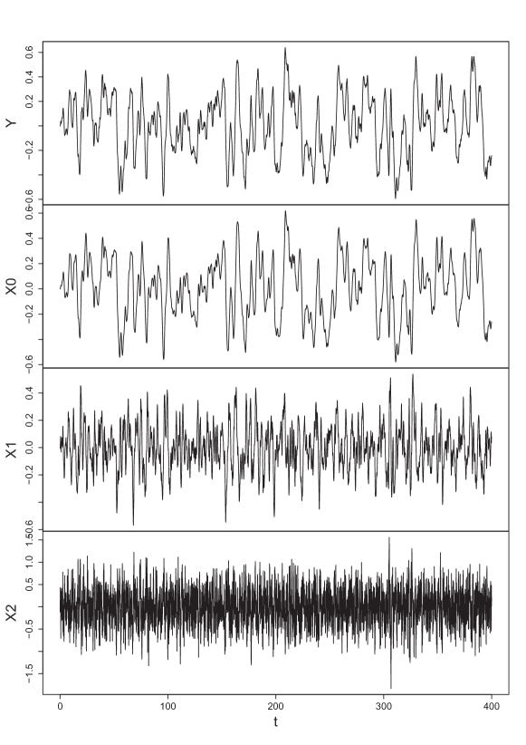
Figure 1: Simulated sample path of a CARMA(3,1) process driven by a standard Browniam motion

Insert here figure 1.

4.3 Estimation of a CARMA model

In this Section we explain how to use the qmle method for performing the three steps estimation procedure described in Sect. 3 for the CARMA(p,q) model. As reported in [11], the qmle function implemented in yuima package works as similar as possible to the standard mle function in the stats4 package when the model is an object of the yuima.model-class. However the behaviour of the function is slightly different if we considerr an object of the yuima.carma-class. Indeed in this case, the qmle function can be return an object of class mle or and object of class yuima.carma.qmle-class.
This class extends the existing class mle for the stats4 package since it has an adjoint slot which contains the Lévy increments estimated by the new yuima function CarmaNoise.

The arguments in the function qmle are:

qmle(yuima, start, method="BFGS", fixed = list(), print=FALSE,
  lower, upper, joint=FALSE, Est.Incr="Carma.IncPar",aggregation=TRUE ...)

For a complete treatment of the arguments passed to the qmle we refer to the yuima documentation. In this work we focus our attention only on the character-string variable Est.Incr and the logical variable aggregation.
The variable Est.Incr manages the output of the qmle function. The variable Est.Incr assumes the following three values:

• Carma.IncPar that is the default value. In this case the function qmle returns an object of yuima.carma.qmle-class which contains the CARMA parameters obtained by quasi-maximum likelihood procedure, the estimated increments and parameters of the underlying Lévy process. If the CARMA(p,q) model is driven by a standard Browniam motion, the behaviour of the function is identically when Est.Incr="Carma.Inc".

• Carma.Inc The function qmle returns an object of yuima.carma.qmle-class which contains only the CARMA parameters and the estimated Lévy increments.

• Carma.Par In this case the output is an object of mle-class containing the estimated CARMA parameters obtained using the quasi maximum likelihood procedure and the parameters of the Lévy process.

The logical variable aggregation is related to the methodology for the estimation of the Lévy parameter. Indeed if the variable is TRUE, the increments are aggregated in order to obtain the increments on unitary time intervals.

In order to obtain the estimated increments of the underlying Lévy process, the qmle function calls internally the function CarmaNoise. The call is done using the following command:

CarmaNoise(yuima, param, data=NULL)

where the arguments mean:

• yuima is a yuima object or an object of yuima.carma-class.

• param is a list of parameters for the CARMA model.

• data is an object of class yuima.data-class contains the observations available at uniformly spaced time intervals. If data=NULL, the default, the CarmaRecovNoise uses the data in an object of yuima.

Using the same example in Sect. 4.2, we list below the code for estimation of the CARMA(3,1) model:

>  qmle.Carma_brown_mod <- qmle(sim.Carma_brown_mod,start=par.Carma_brown_mod)

Starting qmle for carma ...

 Stationarity condition is satisfied...
 Starting Estimation Increments ...

Starting Estimation parameter Noise ...

The function by default returns an object of class yuima.carma.qmle and we can see the values of estimated parameters applying the utulity summary:

> summary(qmle.Carma_brown_mod)

Two Stage Quasi-Maximum likelihood estimation

Call:
qmle(yuima = sim.Carma_brown_mod, start = par.Carma_brown_mod)

Coefficients:
      Estimate  Std. Error
b0 0.975548500 0.010311774
b1 0.226960222 0.002573738
a3 1.736966408 0.003086911
a2 4.964930880         NaN
a1 3.908449535 0.002654231
c0 0.005858153 0.027901534

-2 log L: -178729.2


Number of increments: 15997

Average of increments: -0.000016

Standard Dev. of increments: 0.160054

Summary statistics for increments:
      Min.    1st Qu.     Median       Mean    3rd Qu.       Max.
-0.6159000 -0.1064000 -0.0013330 -0.0000156  0.1093000  0.6150000

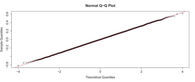
Figure 2: QQ-norm of the estimated increments of the underlying Lévy process.

Since the driven noise is a standard brownian motion, then the estimated parameters are only the autoregressive and moving average parameters. In figure 2 we check the normality from a qualitative point of view using the QQ-norm.

Insert here figure 2.

The behaviour of the QQ-norm seems to confirm that the estimated increments are generated from a normal distribution.

4.4 ctarma package

We conclude this Section by comparing the procedures illustrated before with the corresponding ones avaliable in the ctarma package. As shown in the introduction, the ctarma package developed by [30] contains several routines for the simulation and the estimation of a Gaussian CARMA(p,q) model using both frequency and time-domain approaches. Since in this paper we focus on the state-space representation of a CARMA(p,q) model, we conduct our comparison considering only the time-domain approach and refer to [29] for a complete and detailed explanation of the frequency-domain approach for the simulation and the estimation of a Gaussian CARMA(p,q) model.
Our comparison is based on two exercises. In the first, we build an object of class yuima that contains a simulated sample path of a Gaussian CARMA(2,1) model. We write a simple function that converts an object of class yuima into an object of class ctarma and use this object for the estimation of the CARMA(2,1) parameters applying the ctarma function ctarma.maxlik that performs a maximum likelihood estimation procedure based on the Kalman Filter. We compare these results with those obtained using the qmle function.
In the second exercise we repeat a similar experiment but in this case we simulate a trajectory of a Gaussian CARMA(2,1) using the ctarma function carma.sim.timedomain.

As first step, we simulate a trajectory of a CARMA(2,1) model using the following yuima functions

> mod.yuima<-setCarma(p=2,q=1,scale.par="sig",Carma.var="y")
> param.yuima<-list(a1=1.39631,a2=0.05029,b0=1,b1=1,sig=1)
> samp.yuima<-setSampling(Terminal=100,n=200)
> set.seed(123)
> sim.yuima<-simulate(mod.yuima,true.parameter=param.yuima,sampling=samp.yuima)

We estimate the parameters using the qmle function.

> carmaopt.yuima<-qmle(sim.yuima,start=param.yuima)

Starting qmle for carma ...

 Stationarity condition is satisfied...
 Starting Estimation Increments ...

Starting Estimation parameter Noise ...

> summary(carmaopt.yuima)

Two Stage Quasi-Maximum likelihood estimation

Call:
qmle(yuima = sim.yuima, start = param.yuima)

Coefficients:
     Estimate Std. Error
sig 2.2114666  1.9361348
b0  1.0000000  0.0000000
b1  0.5493488  0.4138758
a2  0.4223176  0.4298420
a1  3.3439956  2.4968459

-2 log L: 403.5426


Number of increments: 198

Average of increments: 0.007277

Standard Dev. of increments: 0.609316

Summary statistics for increments:
     Min.   1st Qu.    Median      Mean   3rd Qu.      Max.
-1.536000 -0.379400 -0.034040  0.007277  0.383400  1.760000

We write a simple function that converts an object of class yuima into an object of class ctarma:

> yuimaToctarma<-function(yuima,true.param){
+   if(("ctarma" %in% rownames(installed.packages()))==FALSE){
+     warning("You need to install ctarma package")
+     return(NULL)
+   }else{
+     require(ctarma)
+   }
+   if(!is(yuima,"yuima")){
+     warning("The model is not an object of class yuima")
+     return(NULL)
+   }
+   model<-yuima@model
+   if(!is(model,"yuima.carma")){
+     warning("The model is not an object of class yuima.carma")
+     return(NULL)
+   }
+   par.names<-names(true.param)
+   par<-as.numeric(true.param)
+   names(par)<-par.names
+   info<-model@info
+   p<-info@p
+   if(length(info@loc.par)!=0){
+     warning("It is not possible to convert a CARMA model with location parameter")
+     return(NULL)
+   }
+   name.ar<-paste(info@ar.par,c(1:p),sep="")
+   a<-true.param[name.ar]
+   q<-info@q
+   name.ma<-paste(info@ma.par,c(0:q),sep="")
+   b<-true.param[name.ma]
+   if(length(info@scale.par)==0){
+     sigma<-1
+   }else{
+     sigma<-par[info@scale.par]
+   }
+
+   data<-yuima@data@zoo.data[[1]]
+   time<-index(data)
+   y<-coredata(data)
+
+   ctarma.mod<-ctarma(ctarmalist(y,time,a,b,sigma))
+   return(ctarma.mod)
+ }

Applying the function yuimaToctarma we obtain an object of class ctarma and estimate the model using the function ctarma.maxlik:

> ctarma.mod<-yuimaToctarma(sim.yuima,param.yuima)
> carmaopt.ctarma<-ctarma.maxlik(ctarma.mod)
> summary(carmaopt.ctarma)

$coeff
               MLE   STD-MLE
AHAT_1   3.3447171 3.2148525
AHAT_2   0.4224339 0.5915801
B_0      1.0000000 0.0000000
BHAT_1   0.5492208 0.4104583
SIGMAHAT 2.2120532 0.3805180

$loglik
[1] -201.7713

$bic
[1] 424.7558

Now we simulate a trajectory using the carma.sim.timedomain function available in the ctarma package.

> a<-c(1.39631, 0.05029)
> b<-c(1,1)
> sigma<-1
> tt<-(1:200)/2
> set.seed(123)
> y<-carma.sim.timedomain(tt,a,b,sigma)

We build an object of class ctarma and we estimate the model parameters using the following command lines:

> ctarma.mod1<-ctarma(ctarmalist(y,tt,a,b,sigma))
> carmaopt.ctarma1<-ctarma.maxlik(ctarma.mod1)
> summary(carmaopt.ctarma1)

$coeff
               MLE    STD-MLE
AHAT_1   0.8290442 0.53687971
AHAT_2   0.0314847 0.05127615
B_0      1.0000000 0.00000000
BHAT_1   2.6821254 1.91361886
SIGMAHAT 0.3406472 0.10815623

$loglik
[1] -176.6141

$bic
[1] 374.4215

We build now an object of class yuima.data using the constructor setData

> yuima.data<-setData(zoo(x=matrix(y,length(y),mod.yuima@equation.number),order.by=tt))

We build an object of class yuima using the constructor setYuima and we apply to it the qmle function in order to estimate the parameters of the model:

> yuima.mod1<-setYuima(data=yuima.data, model=mod.yuima)
> carmaopt.yuima1<-qmle(yuima.mod1,start=param.yuima)

Starting qmle for carma ...

 Stationarity condition is satisfied...
 Starting Estimation Increments ...

Starting Estimation parameter Noise ...

> summary(carmaopt.yuima1)

Two Stage Quasi-Maximum likelihood estimation

Call:
qmle(yuima = yuima.mod1, start = param.yuima)

Coefficients:
      Estimate Std. Error
sig 0.34107952 0.23452372
b0  1.00000000 0.00000000
b1  2.67881403 1.78368917
a2  0.03153544 0.03349193
a1  0.82963964 0.38604787

-2 log L: 353.2283

Number of increments: 197

Average of increments: 0.054225

Standard Dev. of increments: 0.633237

Summary statistics for increments:
    Min.  1st Qu.   Median     Mean  3rd Qu.     Max.
-1.50000 -0.40790  0.02810  0.05422  0.43980  2.09000

In table 1 we summarize the results of our comparison:

First Exercise
Package	yuima		ctarma
Param.	Estimates	s.d	Estimates	s.d
$\sigma$	2.211	1.936	2.212	0.38
$b_{0}$	1.000	Fixed	1.000	Fixed
$b_{1}$	0.549	0.413	0.549	0.41
$a_{2}$	0.422	0.429	0.422	0.591
$a_{1}$	3.343	2.496	3.344	3.214
log L	-201.726		-201.771
Second Exercise
Package	yuima		ctarma
Param.	Estimates	s.d	Estimates	s.d
$\sigma$	0.341	0.234	0.341	0.108
$b_{0}$	1.000	Fixed	1.000	Fixed
$b_{1}$	2.678	1.783	2.682	1.913
$a_{2}$	0.031	0.033	0.031	0.051
$a_{1}$	0.829	0.386	0.829	0.536
log L	-176.614		176.614

Table 1: Comparison between estimation results obtained using yuima and ctarma packages.

Looking at table 1 we observe that the estimates of parameters using the two packages are similar. The differences can be justified from fact that in the ctarma package the stationarity can be enforced using two different one-to-one transformations of the original parameters proposed by [3] and [23] respectively while in the yuima there are no stationarity constraints and the stationarity is checked once the estimates are obtained.
Although both transformations in the ctarma allow to formulate the maximum likelihood estimation as an unconstrained optimization problem on the new variables, the choice in the yuima is justified by the following two reasons:

• The optimization problem is defined on the original autoregressive and moving avarege parameters and this is coherent with the spirit of the Yuima project.

• Defining the optimization problem on the original variables allows the user to manage efficiently the possibility of having constraints on the model parameters.

5 Simulation and estimation of a CARMA(p,q) model driven by a Lévy process

In this Section we show how to simulate and estimate a CARMA(p,q) model driven by a Lévy process in the yuima package. Based on our knowledge, yuima is the first package available on CRAN that allows the user to manage, in a complete way, a Lévy CARMA model. As shown in Sect. 4, it is also possible to recover the increments of the underlying Lévy and consequently the user can build on it a non-parametric Lévy CARMA model, i.e. a model where the distribution of the increments is not specified.
In order to test the procedures implemented in yuima for the simulation and the estimation of a CARMA(2,1) model we consider three different exercises:

• We simulate a trajectory from a CARMA(2,1) driven by a Compound Poisson process with normally distributed jumps and then we use this trajectory for the estimation procedure.

• We repeat a similar exercise and assume that the underlying Lévy process is a Variance Gamma model [22].

• In the last experiment, we assume the underlying Lévy process to be a Normal Inverse Gaussian model [1].

It is worth to notice that since all the considered models can be seen as mixture of normals, the maximum likelihood estimation could be efficiently performed through an EM algorithm as that proposed in [14] and used for the Compound Poisson [19], the Variance Gamma [21] and the Normal Inverse Gaussian [16]. We prefer to maximize directly the log-likelihood function and the densities are computed via Inverse Fourier Transforms. We leave the estimation procedure based on the EM algorithm for future developments of the yuima package.

First example:
We consider a CARMA(2,1) driven by a Compound Poisson where jump size is normally distributed and $\lambda$ is equal to 1.

> modCP<-setCarma(p=2,q=1,Carma.var="y",
+                 measure=list(intensity="Lamb",df=list("dnorm(z, mu, sig)")),
+                 measure.type="CP")
> true.parmCP <-list(a1=1.39631,a2=0.05029,b0=1,b1=2,
+                   Lamb=1,mu=0,sig=1)

We obtain a sample path of the model using the yuima’s simulate function.

> samp.L<-setSampling(Terminal=200,n=4000)
> set.seed(123)
> simCP<-simulate(modCP,true.parameter=true.parmCP,sampling=samp.L)
> plot(simCP,main="CP CARMA(2,1) model",type="l")

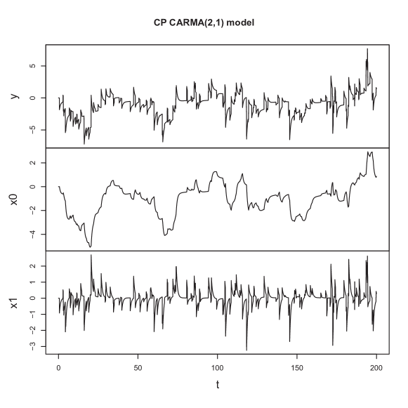
Figure 3: Simulated sample path of a CARMA model driven by a Compound Poisson process. The jump size is normally distributed.

Insert here figure 3.

We estimate the parameter using the three step procedure described in Sect. 3.

> carmaoptCP <- qmle(simCP, start=true.parmCP)

Starting qmle for carma ...

 Stationarity condition is satisfied...
 Starting Estimation Increments ...

Starting Estimation parameter Noise ...

> summary(carmaoptCP)

Two Stage Quasi-Maximum likelihood estimation

Call:
qmle(yuima = simCP, start = true.parmCP)

Coefficients:
         Estimate  Std. Error
b0    0.783877655 0.253566362
b1    1.827108561 0.021281824
a2    0.078614454 0.046810522
a1    1.384434622 0.229686130
Lamb  1.038752541 0.103628795
mu   -0.005414145 0.005461136
sig   0.984266035 0.006756150

-2 log L: 4006.412


Number of increments: 3998

Average of increments: -0.004651

Standard Dev. of increments: 0.218475

-2 log L of increments: 432.210758

Summary statistics for increments:
      Min.    1st Qu.     Median       Mean    3rd Qu.       Max.
-3.1580000 -0.0051220 -0.0015580 -0.0046510  0.0007187  2.7260000

> plot(carmaoptCP,main="Compound Poisson with normal jump size",ylab="Incr.",type="l")

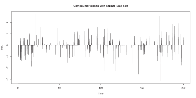
Figure 4: Estimated Lévy Increments for a Carma model driven by a Compound Poisson process.

Insert here figure 4.

Second Example:
In this case, the underlying Lévy is a Variance Gamma model and we instruct yuima to build a CARMA(2,1) process with the following command line:

> modVG<-setCarma(p=2,q=1,Carma.var="y",
+                 measure=list("rngamma(z,lambda,alpha,beta,mu)"),measure.type="code")
> true.parmVG <-list(a1=1.39631, a2=0.05029, b0=1, b1=2,
+                    lambda=1, alpha=1, beta=0, mu=0)

We simulate a trajectory as follows:

> set.seed(100)
> simVG<-simulate(modVG, true.parameter=true.parmVG, sampling=samp.L)
> plot(simVG,main="VG CARMA(2,1) model",type="l")

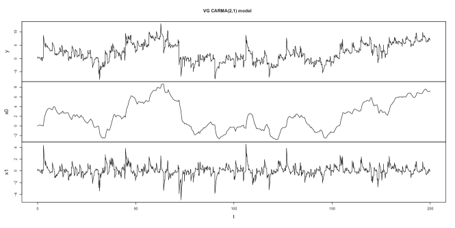
Figure 5: Simulated sample path of a CARMA model driven by a Compound Poisson process. The jump size is normally distributed.

Insert here figure 5.

Applying the qmle function we get

> carmaoptVG <- qmle(simVG, start=true.parmVG)

Starting qmle for carma ...

 Stationarity condition is satisfied...
 Starting Estimation Increments ...

Starting Estimation parameter Noise ...

> summary(carmaoptVG)

Two Stage Quasi-Maximum likelihood estimation

Call:
qmle(yuima = simVG, start = true.parmVG)

Coefficients:
          Estimate Std. Error
b0      1.39902454 0.41767662
b1      2.89637615 0.03385217
a2      0.04582997 0.03307549
a1      1.44727320 0.24192786
lambda  1.04555597 0.26067994
alpha   1.49836490 0.25063939
beta   -0.04555458 0.08291164
mu      0.14534591 0.03540655

-2 log L: 7692.227

Number of increments: 3998

Average of increments: 0.005215

Standard Dev. of increments: 0.218392

-2 log L of increments: 524.119054

Summary statistics for increments:
      Min.    1st Qu.     Median       Mean    3rd Qu.       Max.
-3.0330000 -0.0025170 -0.0001629  0.0052150  0.0026890  2.9550000

> plot(carmaoptVG,main="Variance Gamma increments",ylab="Incr.",xlab="Time",type="l")

Insert here figure 6.

Third Example:
In the third example we assume that the underlying Lévy is a Normal Inverse Gaussian process. As a first step we define a CARMA(2,1) process using the yuima constructor setCarma:

> modNIG<-setCarma(p=2,q=1,Carma.var="y",
+                  measure=list("rNIG(z,alpha,beta,delta1,mu)"),measure.type="code")

In this case we build explicity the underlying Lévy process using the yuima package

> IncMod<-setModel(drift="0",diffusion="0",jump.coeff="1",
+                  measure=list("rNIG(z,1,0,1,0)"),measure.type="code")
> set.seed(100)
> simLev<-simulate(IncMod,sampling=samp.L)
> incr.lev<-diff(as.numeric(simLev@data@zoo.data$Series))
> plot(incr.lev,main="simulated noise increments",type="l")

Insert here figure 7.

The simulated Lévy increments are necessary for building the sample path of the CARMA(2,1) model driven by a Normal Inverse Gaussian process. In yuima package, we simulate a trajectory using the code listed below:

> true.parmNIG <-list(a1=1.39631,a2=0.05029,b0=1,b1=2,
+                   alpha=1,beta=0,delta1=1,mu=0)
> simNIG<-simulate(modNIG,true.parameter=true.parmNIG,sampling=samp.L)

Applying the two steps procedure we obtain the following result:

> carmaoptNIG <- qmle(simNIG, start=true.parmNIG)

Starting qmle for carma ...

 Stationarity condition is satisfied...
 Starting Estimation Increments ...

Starting Estimation parameter Noise ...

> summary(carmaoptNIG)

Two Stage Quasi-Maximum likelihood estimation

Call:
qmle(yuima = simNIG, start = true.parmNIG)

Coefficients:
          Estimate Std. Error
b0      1.45563876 0.57914335
b1      1.96734358 0.02336632
a2      0.08624902 0.05545456
a1      1.64048955 0.41504117
alpha   1.24223088 0.39987929
beta    0.16177182 0.18718818
delta1  1.23129950 0.31792981
mu     -0.23920126 0.16707800

-2 log L: 4610.315

Number of increments: 3998

Average of increments: -0.004164

Standard Dev. of increments: 0.218789

-2 log L of increments: 555.416356

Summary statistics for increments:
     Min.   1st Qu.    Median      Mean   3rd Qu.      Max.
-3.138000 -0.050620 -0.001853 -0.004164  0.041450  3.283000

> plot(carmaoptNIG,main="Normal Inverse Gaussian",ylab="Incr.",type="l")

Insert here figure 8.

In the end of this Section, we show how to estimate the parameters of the underlying Normal Inverse Gaussian Lévy process using the package GeneralizedHyperbolic and discuss the accuracy of the estimates obtained using the qmle function.

As a first step, we get the Lévy shock from an object of class yuima.carma.qmle

> NIG.Inc<-as.numeric(coredata(carmaoptNIG@Incr.Lev))
> NIG.freq<-frequency(carmaoptNIG@Incr.Lev)

We aggregate the innovations in order to obtain the increments on the interval with unit length.

> Unitary.NIG.Inc<-diff(cumsum(NIG.Inc)[seq(from=1, to=length(NIG.Inc), by=NIG.freq)])

The function nigFit, available in the package Generalized Hyperbolic, fits a Normal Inverse Gaussian distribution to the data Unitary.NIG.Inc maximizing the log-likelihood function. The function returns an S3 object of class nigFit.

> library(GeneralizedHyperbolic)
> FitInc.NIG.Lev<-nigFit(Unitary.NIG.Inc)
> summary(FitInc.NIG.Lev, hessian = TRUE, hessianMethod = "tsHessian")

Data:      Unitary.NIG.Inc
Hessian:  tsHessian
               mu      delta      alpha       beta
mu    -246.191203  -9.686779   7.619589 -199.06132
delta   -9.686779 -56.595855  39.612917  -13.39664
alpha    7.619589  39.612917 -34.270069   12.82121
beta  -199.061324 -13.396643  12.821209 -191.77232
Parameter estimates:
       mu        delta       alpha        beta
   -0.15880     1.21181     1.26833     0.08503
  ( 0.16206)  ( 0.30642)  ( 0.39880)  ( 0.18539)
Likelihood:         -272.713
Method:             Nelder-Mead
Convergence code:   0
Iterations:         247

Looking to the summary, differences on the estimates obtained with two methods, qmle and nigFit, are negligibles. In the following figure we report a comparison of the theoretical and empirical log-densities (left side) and a qqplot (right side) obtained using the plot function for an object of class nigFit.

> par(mfrow = c(1, 2))
> plot(FitInc.NIG.Lev, which = 2:3,
+        plotTitles = paste(c("Histogram of NIG ",
+                             "Log-Histogram of NIG ",
+                             "Q-Q Plot of NIG "), "Incr.",
+                           sep = ""))

Insert here figure 9.

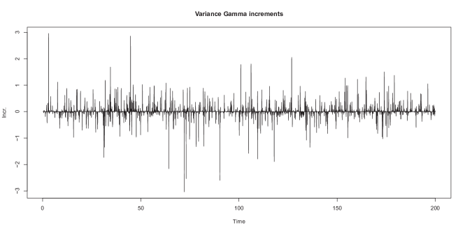
Figure 6: Estimated Lévy increments for a Carma model driven by a Variance Gamma process

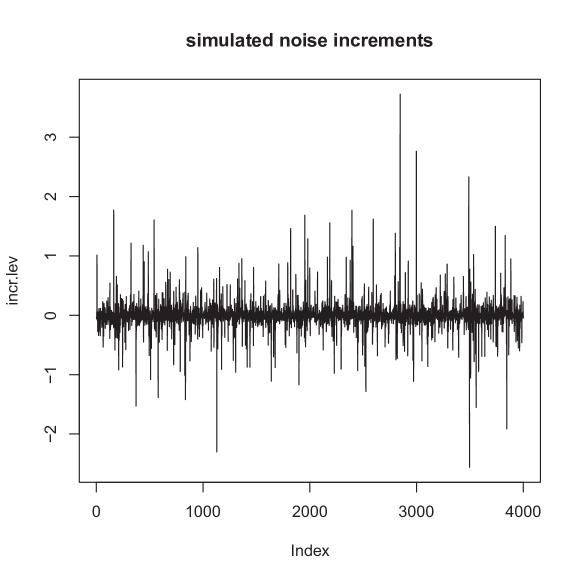
Figure 7: Simulated increments for a Normal Inverse Gaussian process

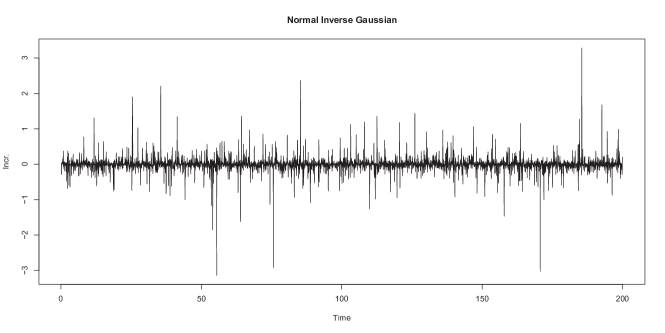
Figure 8: Estimated increments for a Carma model driven by a Normal Inverse Gaussian process

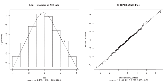
Figure 9: Comparison theoretical and empirical log-density (left side). qq-plot (right side) of the estimated increments. The quantiles used for comparison are computed using the Normal Inverse Gaussian distribution.

References

- [1] O. Barndorff-Nielsen. Exponentially Decreasing Distributions for the Logarithm of Particle Size. Royal Society of London Proceedings Series A, 353, 1977.
- [2] O. E. Barndorff-Nielsen and N. Shephard. Non-gaussian ornstein-uhlenbeck-based models and some of their uses in financial economics. Journal of the Royal Statistical Society Series B, 63(2):167–241, 2001.
- [3] J. Belcher, J. S. Hampton, and G. Tunnicliffe Wilson. Parameterization of continuous time autoregressive models for irregularly sampled time series data. Journal of the Royal Statistical Society. Series B (Methodological), 56(1):141–155, 1994.
- [4] J. Bertoin. Lévy processes, 1998. Cambridge University Press.
- [5] P. Brockwell, E. Chadraa, and A. Lindner. Continuous-time GARCH processes. Annals of Applied Probability, 16(2):790–826, 2006.
- [6] P. J. Brockwell, R. A. Davis, and Y. Yang. Estimation for non-negative lévy-driven ornstein-uhlenbeck processes. Journal of Applied Probability, 44:987–989, 2007.
- [7] P. J. Brockwell, R. A. Davis, and Y. Yang. Estimation for non-negative lévy-driven carma processes. Journal of Business & Economic Statistics, 29(2):250–259, 2011.
- [8] P. J. Brockwell and E. Schlemm. Parametric estimation of the driving lévy process of multivariate carma processes from discrete observations. Journal of Multivariate Analysis, 115:217–251, 2013.
- [9] P.J. Brockwell. Lévy-driven carma processes. Annals of the Institute of Statistical Mathematics, 53(1):113–124, 2001.
- [10] P.J. Brockwell and T. Marquardt. Lévy-driven and fractionally integrated arma processes with continuous time parameter. Statistica Sinica, 15(2):477–494, 2005.
- [11] A. Brouste, M. Fukasawa, H. Hino, S. M. Iacus, K. Kamatani, Y. Koike, H. Masuda, R. Nomura, T. Ogihara, Shimuzu Y., M. Uchida, and Yoshida N. The yuima project: A computational framework for simulation and inference of stochastic differential equations. Journal of Statistical Software, 57(4):1–51, 2014.
- [12] A. Brouste and S. M. Iacus. Parameter estimation for the discretely observed fractional ornstein-uhlenbeck process and the yuima r package. Comput Stat, 28:1529–1547, 2013.
- [13] J.M. Chambers. Programming with data: A Guide to the S Language., 1998. Springer-Verlag New York.
- [14] A. P. Dempster, N. M. Laird, and D. B. Rubin. Maximum likelihood from incomplete data via the em algorithm. Journal of the Royal Statistical Society. Series B (Methodological), 39(1):1–38, 1977.
- [15] R development Core Team. A language and environment for statistical computing. R foundation for statistical computing., 2010. Vienna Austria.
- [16] K. Dimitris. An {EM} type algorithm for maximum likelihood estimation of the normal-inverse gaussian distribution. Statistics & Probability Letters, 57(1):43 – 52, 2002.
- [17] J.L. Doob. The elementary gaussian process. Ann. Math. Stat., 15(3):229–282, 1944.
- [18] C. Francq and J.-M. Zakoïan. Estimating linear representations of nonlinear processes. Journal of Statistical Planning and Inference, 68:145–165, 1998.
- [19] J. Hinde. Compound Poisson regression models., 1982. GLIM 82: Proceedings of the International Conference on Generalised Linear Models. Springer New York.
- [20] R.M. Kalman. A new approach to linear filtering and prediction problems. Journal of Basic Engineering Transactions of the ASME. Serie D, 82:35–45, 1960.
- [21] A. Loregian, L. Mercuri, and E. Rroji. Approximation of the variance gamma model with a finite mixture of normals. Statistics & Probability Letters, 82(2):217 – 224, 2012.
- [22] D. B. Madan and E. Seneta. The variance gamma (v.g.) model for share market returns. The Journal of Business, 63(4):511–24, 1990.
- [23] D. T. Pham and A. Breton. Levinson-durbin-type algorithms for continuous-time autoregressive models and applications. Mathematics of Control, Signals and Systems, 4(1):69–79, 1991.
- [24] K. Sato. Lévy processes and infinitely divisible distributions, 1999. Cambridge University Press.
- [25] E. Schlemm and R. Stelzer. Quasi maximum likelihood estimation for strongly mixing state space models and multivariate lévy-driven carma processes. Electronic Journal of Statistics [electronic only], 6:2185–2234, 2012.
- [26] YUIMA Project Team. yuima: The YUIMA Project package (stable version), 2013. R package version 1.0.2.
- [27] V Todorov. Econometric analysis of jump-driven stochastic volatility models. Journal of Econometrics, 160(1):12–21, 2011.
- [28] V. Todorov and G. Tauchen. Simulation methods for levy-driven continuous-time autoregressive moving average (carma) stochastic volatility models. Journal of Business & Economic Statistics, 24:455–469, 2006.
- [29] H. Tomasson. Some computational aspects of gaussian carma modelling. Statistics and Computing, pages 1–13, 2013.
- [30] Helgi Tomasson. ctarma: Estimation and simulation of CARMA(p,q), 2013. R package version 0.1.5.
- [31] H. Tsai and K. Chan. A note on the covariance structure of a continuous-time arma process. Statistica Sinica, 10(3):989–998, 2000.
- [32] Granville Tunnicliffe-Wilson and Alex Morton. Modelling multiple time series: Achieving the aims. In Jaromir Antoch, editor, COMPSTAT 2004 - Proceedings in Computational Statistics, pages 527–538. Physica-Verlag HD, 2004.
- [33] Z. Wang. cts: An R package for continuous time autoregressive models via kalman filter. Journal of Statistical Software, 53(5):1–19, 2013.