An Information-Theoretic Formalism for Multiscale Structure in Complex Systems

Abstract

We develop a general formalism for representing and understanding structure in complex systems. In our view, structure is the totality of relationships among a system’s components, and these relationships can be quantified using information theory. In the interest of flexibility we allow information to be quantified using any function, including Shannon entropy and Kolmogorov complexity, that satisfies certain fundamental axioms. Using these axioms, we formalize the notion of a dependency among components, and show how a system’s structure is revealed in the amount of information assigned to each dependency. We explore quantitative indices that summarize system structure, providing a new formal basis for the complexity profile and introducing a new index, the “marginal utility of information”. Using simple examples, we show how these indices capture intuitive ideas about structure in a quantitative way. Our formalism also sheds light on a longstanding mystery: that the mutual information of three or more variables can be negative. We discuss applications to complex networks, gene regulation, the kinetic theory of fluids and multiscale cybernetic thermodynamics.

I Introduction

I.1 Overview

The field of complex systems seeks to identify, understand and predict common patterns of behavior across the physical, biological and social sciences baryam2003 ; haken2006 ; millerpage2007 ; boccara2010 ; newman2011 . It succeeds by tracing these behavior patterns to the structures of the systems in question. We use the term “structure” to mean the totality of quantifiable relationships among the components comprising a system. Systems from different domains and contexts can share key structural properties, causing them to behave in similar ways. For example, the central limit theorem tells us that we can sum over many independent random variables and obtain an aggregate value whose probability distribution is well-approximated as a Gaussian. This helps us understand systems composed of statistically independent components, whether those components are molecules, microbes or human beings. Likewise, different chemical elements and compounds display essentially the same behavior near their respective critical points. The critical exponents which encapsulate the thermodynamic properties of a substance are the same for all substances in the same universality class, and membership in a universality class depends upon structural features such as dimensionality and symmetry properties, rather than on details of chemical composition sethna2006 ; ncatlab-universality .

Mathematical representations of systems encode different aspects of structure baryam2003 ; millerpage2007 ; castellano2009 ; boccara2010 . Common representations include networks (watts1998, ; barabasi1999, ; strogatz2001, ; newman2003networks, ; wang2003, ; watts2003, ; boccaletti2006networks, ; dorogovtsev2010, ), lattice models and cellular automata (chopard1998cellular, ; hoekstra2010, ; stacey2011, ), interacting agent models liggett1985interacting ; durrett1994 ; axelrod1997complexity ; helbing2001traffic ; bonabeau2002 , differential equations mackey1977oscillation , difference equations may1976simple ; ott1981 and continuum field theories turing1952 ; cross1993pattern ; maini1997spatial . While mathematical inference is a rigorous aspect of science once a mathematical model is identified, the choice of representation for a particular system or class of systems often relies upon an ad hoc leap of intuition. The task of constructing useful representations becomes challenging for complex systems, where the set of system components is not just large, but also interwoven and resistant to decomposition. Indeed, the set of system components for real-world physical, biological or social entities can be expected to be so intricate that, for all practical purposes, precise enumeration is ultimately intractable. Achieving a fundamental solution to this problem is critical for our ability to empower theoretical physics as a general approach to complex systems, and a practical solution is critical for our ability to address many real-world challenges.

An important clue about how to achieve a general solution is found in the renormalization group analysis of phase transitions, a prototype for complex-systems thinking. According to this analysis, we can characterize analytically the set of “relevant” parameters that are necessary and sufficient to characterize the behavior of a system in the thermodynamic limit. This provides a formal conceptual basis for discarding variables which are unnecessary for a successful practical description. In addition, it furnishes a formal approach to obtaining those variables, eliminating the ad hoc aspects of constructing models. Generalizing this approach requires an understanding of information theory in a multiscale context, a context that has not been developed in information theory nor in the statistical physics of phase transitions. In particular we need a formal and general understanding of how mathematical representations capture the structure of systems, i.e., the information that characterizes the set of possible configurations or behaviors of a system. We must also consider the fundamental nature of the concept of scale in order to distinguish, where appropriate, finer-scale details that can be selectively neglected in favor of larger-scale ones.

These issues underline the need to develop a generalized mathematical framework for discussing the multiscale structure of systems that builds on information theory. Here we develop such a framework, incorporating a set of complex-systems ideas, which can anchor discussions of mathematical representation and formalize our intuitive notion of system structure. Our formalism applies to any system for which a suitable quantitative measure of information can be defined.

The need for such a theory is also apparent from the lack of a quantitative notion of a “complex system” as distinguished from other varieties of systems. It makes intuitive sense that quantitatively defining system complexity should enable the identification of complex systems. However, efforts to define complexity encounter a paradox. One might think to quantify system complexity using measures like Kolmogorov/algorithmic complexity or Shannon information that quantify irregularity or unpredictability in an object or a stochastic process. However, the systems deemed the most “complex” by these indices are those in which the components behave independently of each other, such as ideal gases. Such systems lack the multiscale regularities and interdependencies that characterize the systems typically studied by complex systems researchers.

Some theorists have argued that true complexity is best viewed as occupying a position between order and randomness grassberger1986 ; crutchfield1989 ; crutchfield1994 . Music is, so the argument goes, intermediate between still air and white noise. This answer is unsatisfying, however. Though complex systems contain both order and randomness, they do not appear to be mere blends of the two. For example, a box containing both a crystal and an ideal gas is a system with intermediate entropy, but would not normally be considered a complex system. In a truly complex system, the balance of order and randomness is captured in the multiscale relationships among the system’s components—that is, in the system’s structure. Hence, we are brought to the realization that a formal theory of structure based upon a generalization of information theory is critical for understanding what complexity is and for characterizing the essential attributes of complex systems.

We begin by outlining, in Section II, the properties which such an information function must satisfy. Examples include, but are not limited to, Shannon information, algorithmic complexity, and vector space dimension. We require only minimal assumptions so that our formalism can apply as broadly as possible.

In Section III, we formalize the notion of a system and introduce illustrative examples to which we will refer throughout the work. Section IV introduces the central notion of a dependency space—a Venn diagram or Euler diagram representation of inter-component relationships. Section V sets out the idea of a subsystem—one system embedded within another—and Section VI formalizes the idea of scale, elaborating how to quantify multiscale relationships via information theory.

This development culminates in Section VII, which discusses two indices of multiscale structure: the complexity profile baryam2004b and a new index, the marginal utility of information (MUI). These indices resolve the paradox of complexity, order and randomness, by showing how information and complexity can exist at multiple scales. The systems of greatest interest to the complex systems community are those displaying nontrivial complexity at a wide range of scales. Section VIII develops a combinatorial formula for the complexity profile and related quantities.

In Section IX we consider special classes of systems for which the indices introduced in Section VII take a simplified form. We use these systems to illustrate important properties of the two indices. Section X builds on these ideas to study systems acted upon by external agents, using multicylinder Szilárd engines as an illustrative example. Finally, Section XI presents our general conclusions and outlines directions for future work. This section discusses related concepts including negentropy, requisite variety and their implications for the scientific characterization of complex systems.

I.2 List of key concepts

• System: A system is an entity composed of constituent parts, which we call components. Systems can be dynamic or static, deterministic or probabilistic.

• Information: Information quantifies the degree of freedom, irregularity or unpredictability of a set of components. Specific measures of information can be chosen depending on the type of representation available for the system, or for different purposes. In each context, an information measure indicates how many questions one needs answered to remove uncertainty about the system components under consideration. Though different measures of information are computed differently and require different types of data, they share certain fundamental mathematical properties, which we outline in Section II.

• Dependency: A dependency among a set of components is the relationship (if any) among them causing information pertinent to one component to be pertinent to them all. We introduce a new notation for dependencies; for example, the dependency among components $a$, $b$, and $c$ is denoted $a;b;c$. We also consider conditional dependencies such as $a;b|c$, which stands for the relationship between $a$ and $b$ that exist independently of their relationships with $c$. The strength of the relationships that comprise a dependency can be quantified using information theory. For example, the conditional mutual information $I(a;b|c)$ quantifies how strongly $a$ and $b$ are related in their behavior, excluding effects attributable to $a$ and $b$’s mutual relationships with $c$.

• Structure: A system’s structure is the totality of relationships among all sets of components, or, equivalently, the collection of all dependencies in the system. We can characterize structure quantitatively in terms of the amounts of information assigned to each dependency. Since this definition of structure makes no reference to the nature of the components or the mechanisms by which they interact, the structures of systems from very different contexts can be analyzed and compared using this framework.

• Scale: Relative size plays a central role in understanding and quantifying structure. The scale of a system behavior is given by the number of components that are engaged in that behavior. Formally, scale is the number of components involved in a dependency of the system. The extent of system behavior at a particular scale is quantified by the amount of information assigned to dependencies at this scale. Information and scale are complementary: As information is about the degree of freedom, scale is about constraints associated with redundancy. A large-scale behavior requires redundant information among the many components engaged in that behavior.

• Indices of Structure: Since systems with many components involve a large number of dependencies, the full structure of a system can be unwieldy to represent. We develop two indices which give summary characterizations of a system’s overall structure. The first is the complexity profile, an expression of the tradeoff between complexity and coordination introduced in prior work baryam2004b . The second is a new measure, the marginal utility of information (MUI). These indices characterize, respectively, the amount of information that is present in the system behavior at different scales, and the descriptive utility of limited information through its ability to describe behavior of multiple components.

II Information

In defining the concept of structure we make use of a measure of information. Conceptually, information specifies a particular entity out of a set of possibilities and thus enables us to describe or characterize that entity. A measure of information characterizes the amount of information needed. Rather than adopting a specific information measure, we consider that the amount of information may be quantified in different ways, each appropriate to different contexts. To unify these measures, we develop an axiomatically based approach that considers a generalized information function satisfying two axioms. These axioms are satisfied by Shannon information and algorithmic complexity among others. We use the information function to map out how information is shared among components of a system. This sharing—in which information about some components can be gained by examining others—is central to our discussion of structure.

Let $A$ be the set of components in a system. An information function, $H$, assigns a nonnegative real number to each subset $U\subset A$, representing the amount of information needed to describe the components in $U$. We require that such a function satisfy two axioms:

• Monotonicity: The information in a subset $U$ that is contained in a subset $V$ cannot have more information than $V$, that is, $H(U)\leq H(V)$.

• Strong subadditivity: Given two subsets, the information contained in both cannot exceed the information in each of them separately minus the information in their intersection:

  $$H(U\cup V)\leq H(U)+H(V)-H(U\cap V).$$ (1)

Strong subadditvity expresses how information combines when parts of a system ($U$ and $V$) are regarded as a whole ($U\cup V$). Information regarding $U$ may overlap with information regarding $V$ for two reasons. First, $U$ and $V$ may share components; this is corrected for by subtracting $H(U\cap V)$. Second, constraints in the behavior of non-shared components may reduce the information needed to describe the whole. Thus, information describing the whole may be reduced due to overlaps or redundancies in the information applying to different parts, but it cannot be increased. These redundancies are directly related to emergent collective behaviors.

The above axioms are best known in the context of Shannon entropy; however, they apply to a number of measures that quantify information or complexity, and different measures are appropriate for different types of system:

• Microcanonical or Hartley entropy: For a system with a finite number of joint states, $H_{0}(U)=\log m$, where $m$ is the number of joint states available to the subset $U$ of components. Here, information content measures the number of yes-or-no questions which must be answered to identify one joint state out of $m$ possibilities.

• Boltzmann–Shannon entropy: For a system characterized by a probability distribution over all possible joint states, $H(U)=-\sum_{i=1}^{m}p_{i}\log p_{i}$, where $p_{1},\ldots,p_{m}$ are the probabilities of the joint states available to the components in $U$ shannon1948 . Here, information content measures the number of yes-or-no questions which must be answered to identify one joint state out of all the joint states available to $U$, where more probable states can be identified more concisely.

• Algorithmic complexity: For a system whose subsets can each be encoded as character strings, the algorithmic complexity $H(U)$ is the length of a maximally efficient description of $U$ according to some algorithmic scheme. This notion has been formalized in a number of ways. When a subset $U$ can be encoded as a binary string, the algorithmic complexity of $U$ can be quantified as the length of the shortest self-delimiting program producing this string, with respect to some universal Turing machine. Information content then measures the number of machine-language instructions which must be given to reconstruct $U$. While conceptually clean, this definition is problematic. First, the algorithmic complexity is only defined up to a constant which depends on the choice of universal Turing machine. Second, thanks to the halting problem, the algorithmic complexity can only be estimated, not computed exactly. We can establish upper bounds, but not precise values. These difficulties have led to modifications of the algorithmic complexity concept in which the description scheme is less wide-ranging than the set of all Turing machine programs shallit2001 ; calude2009 ; ahnert2010 .

• Logarithm of period: For a deterministic dynamic system with periodic behavior, an information function can be defined as the logarithm of the period of a set of components (i.e., the time it takes for the joint state of these components to return to an initial joint state) steudel2010 . This information function measures the number of questions which one should expect to answer in order to locate the position of those components in their cycle.

• Vector space dimension: For a system the joint states of whose components can be described as points in a vector space, a possible information function is the dimension of the smallest vector space needed to describe the joint states of the components in $U$. This dimension can be computed in practice, for example, by performing a principal components analysis on the variables representing components in $U$ allen2008 . Here, information content measures the number of coordinates one must specify in order to locate the joint state of $U$.

• Matroid rank: A matroid consists of a set of elements called the ground set, together with a rank function that takes values on subsets of the ground set. Rank functions are defined to include the monotonicity and strong subadditivity properties dougherty2007 , and generalize the notion of vector subspace dimension. Consequently, the rank function of a matroid is an information function in our framework, with the ground set identified as the set of system components.

III Systems

III.1 Definitions

We formally define a system $\mathcal{A}$ to be a finite set $A$ of components, together with an information function $H_{\mathcal{A}}$ (in this case and for other definitions, we omit the subscript when only one system is under consideration). The choice of information function will reflect how the system is modeled mathematically, and it affects the kind of statements we can make about its structure.

A subsystem is a smaller system embedded in a larger one. Formally, we define a subsystem of $\mathcal{A}=(A,H_{\mathcal{A}})$ as a pair $\mathcal{B}=(B,H_{\mathcal{B}})$, where $B$ is a subset of $A$ and $H_{\mathcal{B}}$ is the restriction of $H_{\mathcal{A}}$ to subsets of $B$.

III.2 Static, Dynamic, and Probabilistic Systems

Systems can be static (existing in one state only), probabilistic (existing in a number of possible states with associated probabilities), or dynamic (existing in a sequence of states through time). Dynamic systems can be either deterministic or stochastic.

Different information measures are appropriate depending on the static, dynamic or probabilistic nature of the system in question. For example, static systems may be amenable to algorithmic complexity measures, whereas Shannon entropy applies naturally to probabilistic systems. Dynamic systems are most directly addressed as time histories. A single time history can be studied using algorithmic measures, while an ensemble of time histories may be studied using probabilistic measures. Dynamic systems may also be treated as probabilistic systems, using the approach of ergodic theory, wherein the frequencies of occupancy of different states over extended periods of time are treated as a probability distribution. Our framework can then characterize the structure of the system in terms of its statistical behavior over long timescales.

The methods outlined here can be used to explore the dynamics of a system’s structure, using information measures whose values vary as relationships change within a system over time. However, our current work focuses only on structure as an unchanging property of a system.

III.3 Empirically motivated examples

Our framework can be applied to a wide variety of real-world complex systems. We highlight four in particular:

• Gene regulatory systems: Genes within a cell change over time in their expression levels, i.e., their rate of protein or RNA production. Proteins produced by one gene may promote or inhibit the expression of other genes; thus, genes are an interdependent system with regard to their expression levels jacob1961 ; britten1969gene ; carey2001transcriptional ; elowitz2002stochastic ; lee2002 ; shen2002network ; boyer2005 ; chowdhury2010 . Individual genes can be represented as components of a system, and the information function quantifies the range of behaviors available to sets of genes. Relationships, e.g., promotion or inhibition of one gene by another, can be quantified using mutual information.

• Neural systems: In a nervous system, neurons transmit electrical signals to each other. These signals can be excitatory or inhibitory. If the sum of input signals in a neuron exceeds some activation threshold, this neuron will “fire” and transmit signals to other neurons, promoting or inhibiting their firing in turn hopfield1982neural ; rabinovich2006 . The components are neurons, and the information measure quantifies the range of joint spiking behavior in a collection of neurons (cf. schneidman2006weak ).

• Financial markets: Financial markets are complex interdependent systems mandelbrot1967distribution ; mantegna1999 ; sornette2004stock ; may2008 ; schweitzer2009 ; harmon2010 ; haldane2011systemic ; harmon2011predicting ; misra2011 , where investors can be represented as system components, and the information function quantifies the range of investment activities among a set of investors. Alternatively, one may view the assets as the components, and the information function quantifies the range of joint behavior in the prices of a set of assets.

• Spin systems: Many systems in statistical and condensed-matter physics are represented by considering components arranged on a graph or lattice. The states of these components are characterized by discrete or continuous values, and these values vary stochastically according to which configurations are energetically favorable. The contribution made by an individual component to the system’s total energy depends on its interactions with its neighbors. The prototypical example is the Ising model, in which each component has a “spin”, which can be “up” or “down”, and the interaction energy of a neighboring pair of spins depends on whether they are parallel or antiparallel. Spin-system models play a vital role in the study of magnets, material mixtures such as alloys, liquid-gas phase transitions and other physical systems domb1972 ; baryam2003 ; kardar2007b . The appropriate information function is the Shannon information, which is physically significant owing to the correspondence between Shannon information and thermodynamic entropy feynman1996 ; sgs2004 .

III.4 Simple examples

To illustrate our formalism, we shall use four simple systems as examples.

• Example A: Three independent bits: The system comprises three components, each of which is equally likely to be in state 0 or state 1, and the system as a whole is equally likely to be in any of its eight possible states.

• Example B: Three completely interdependent bits: Each of the three components is equally likely to be in state 0 or state 1, but all three components are always in the same state.

• Example C: Independent blocks of dependent bits: Each component is equally likely to take the value 0 or 1; however, the first two components always take the same value, while the third can take either value independently of the coupled pair.

• Example D: The $2+1$ parity bit system: Three bits which can exist in the states 110, 101, 011, or 000 with equal probability. Each of the three bits is equal to the parity (0 if even; 1 if odd) of the sum of the other two. Any two of the bits are statistically independent of each other, but the three as a whole are constrained to have an even sum.

IV Dependencies

Structure in complex systems reflects the observation that components are not independent of each other. This lack of independence implies that the behavior or state of a component may then be inferred, in whole or in part, from the behaviors or states of others. We illustrate this principle with three examples:

• In the Example C above, the state of the first component is determined by the state of the second, and vice versa. In contrast, the state of the third component cannot be obtained from, nor used to obtain, the states of the first two.

• In gene regulatory systems, the expression level of a gene may be determinable, in whole or in part, from the expression level of other genes that have regulatory interactions with this gene.

• In a fixed structure such as a building, the components (e.g., bricks, windows, etc.) are located in fixed spatial relationship to each other. If the structure as a whole were moved in three-dimensional space, relative to some point of reference (which can be achieved by moving either the structure or the point of reference), the locations of three components would suffice to determine the locations of all others.

We call relationships such as these dependencies. Such dependencies form the basis for our theory of structure. With this flexible notion of dependencies, our formalism describes not only rigid structures such as a building, but also “soft” structures arising from relationships that are not fully determinate, e.g., statistical or probabilistic relationships. This section introduces a general, information-theoretic language for describing and quantifying dependencies.

IV.1 Notation for dependencies

A dependency among a collection of components $a_{1},\ldots,a_{m}$ is the relationship (if any) among these components such that the behavior of some of the components is in part obtainable from the behavior of others. We denote this dependency by the expression $a_{1};\ldots;a_{m}$. This expression represents a relationship, rather than a number or quantity. We use a semicolon to keep our notation consistent with standard information theory (see below).

We can identify a more general concept of conditional dependencies. Consider two disjoint sets of components $a_{1},\ldots,a_{m}$ and $b_{1},\ldots,b_{k}$. The conditional dependency $a_{1};\ldots;a_{m}|b_{1},\ldots,b_{k}$ represents the relationship (if any) between $a_{1},\ldots,a_{m}$ such that the behavior of some of these components can yield improved inferences about the behavior of others, relative to what could be inferred from the behavior of $b_{1},\ldots,b_{k}$. We call this the dependency of $a_{1},\ldots,a_{m}$ given $b_{1},\ldots,b_{k}$, and we say $a_{1},\ldots,a_{m}$ are included in this dependency, while $b_{1},\ldots,b_{k}$ are excluded.

A system’s dependencies can be organized in a Venn diagram, as in Figure 1. We call this diagram a dependency diagram. Each dependency in a system corresponds to a region of the dependency diagram.

We call a dependency irreducible if every system component is either included or excluded. The irreducible dependencies in a three-component system are pictured in Figure 1. We denote the set of all irreducible dependencies of a system $\mathcal{A}$ by $\mathfrak{D}_{\mathcal{A}}$.

The relationship between the components and dependencies of $\mathcal{A}$ can be captured by a mapping from $A$ to subsets of $\mathfrak{D}_{\mathcal{A}}$. A component $a\in A$ maps to the set of irreducible dependencies that involve $a$ (or in visual terms, the region of the dependency diagram that corresponds to component $a$). We represent this mapping by the function $\delta$. For example, in a system of three components $a$, $b$, $c$, we have

$$\delta(a)=\{(a;b;c),\;(a;b|c),\;(a;c|b),\;(a|b,c)\}.$$ (2)

The parentheses around each dependency are used only to delineate dependencies from each other. We can extend the domain of this function to subsets of components, by mapping each subset $U\subset A$ onto to the set of all irreducible dependencies that involve at least one element of $U$; for example,

$$\delta(\{a,b\})=\{(a;b;c),\;(a;b|c),\;(a;c|b),\;(b;c|a),\;(a|b,c),\;(b|a,c)\}.$$ (3)

Visually, $\delta(\{a,b\})$ is the union of the circles representing $a$ and $b$ in the dependency diagram. Finally, we can extend the domain of this function to dependencies, by mapping the dependency $a_{1};\ldots;a_{m}|b_{1},\ldots,b_{k}$ onto the set of all irreducible dependencies that include $a_{1},\ldots,a_{m}$ and exclude $b_{1},\ldots,b_{k}$; for example,

$$\delta(a|c)=\{(a;b|c),\;(a|b,c)\}.$$ (4)

Visually, $\delta(a|c)$ consists of the regions corresponding to $a$ but not to $c$.

Figure 1: The dependency diagram of a system with three components, $a$, $b$ and $c$, represented by the interiors of the three circles. The seven irreducible dependencies shown above correspond to the seven interior regions of the Venn diagram encompassed by the boundaries of the three circles. Reducible dependencies such as $a|b$ are not shown.

Figure 2: Dependency diagram for example A.

Figure 3: Dependency diagram for example B.

Figure 4: Dependency diagram for example C.

Figure 5: Dependency diagram for the $2+1$ parity bit system, example D.

IV.2 Information quantity in dependencies

If a collection of components are dependent, such that the behavior of some can be inferred from the behavior of others, this is reflected in shared information among these components. For example, in a system of random variables, with Shannon entropy as an information function, any statistical dependence between components $a$ and $b$ will cause their joint information $H(a,b)$ to be less than the sum of their separate informations $a$ and $b$, indicating the presence of shared (mutual) information. The amount of shared information quantifies the strength of this dependence. Our formalism for system structure is based on quantifying shared information across subsets of components and multiple scales.

To formalize this idea, we introduce a function $I_{\mathcal{A}}$ that quantifies the shared information in the dependencies of a system $\mathcal{A}$. The values of $I_{\mathcal{A}}$ (the shared information in dependencies) may be derived from the values of the previously defined information function $H_{\mathcal{A}}$, which is the joint information in sets of components. $H_{\mathcal{A}}$ and $I_{\mathcal{A}}$ characterize the same quantity—information—but are applied to different kinds of arguments: $H_{\mathcal{A}}$ is applied to subsets of components of $\mathcal{A}$, while $I_{\mathcal{A}}$ is applied to dependencies.

To mathematically define the shared information $I_{\mathcal{A}}$, we first specify a solvable system of equations that determines its value on irreducible dependencies. For each subset $U\subset A$, we set

$$\sum_{x\in\delta(U)}I(x)=H(U).$$ (5)

As $U$ runs over all subsets of $A$, the resulting system of equations determines the values $I(x)$, $x\in\mathfrak{D}_{\mathcal{A}}$, in terms of the values $H(U)$, $U\subset A$. The solution is an instance of the inclusion-exclusion principle erickson1996 , and can also be obtained by Gaussian elimination. An explicit formula obtained in the context of Shannon entropy yeung1991 applies as well to any information function.

We extend $I$ to dependencies that are not irreducible by defining the shared information $I(x)$ to be equal to the sum of the values of $I(y)$ for all irreducible dependencies $y$ encompassed by a dependency $x$:

$$I(x)=\sum_{y\in\delta(x)}I(y).$$ (6)

More generally, we can extend the shared information $I$ to take, as its argument, any set of irreducible dependencies $D\subset\mathfrak{D}_{\mathcal{A}}$. This is done by setting

$$I(D)=\sum_{y\in D}I(y).$$ (7)

The above relation gives $\mathfrak{D}_{\mathcal{A}}$ the structure of a finite signed measure space, with measure $I$. It is a signed measure space because $I$ can take negative values (see below).

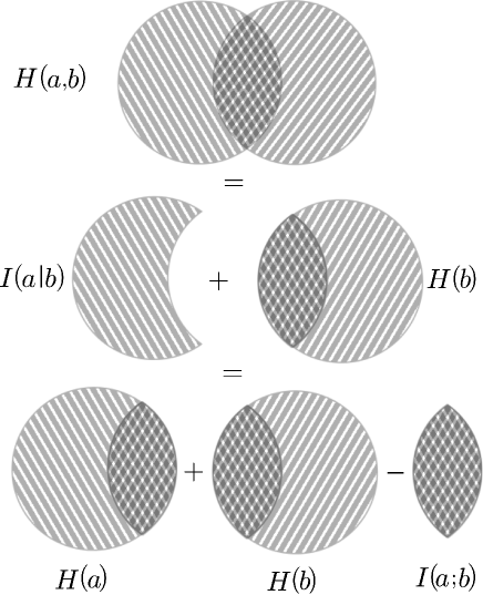
Figure 6: An information diagram for a two-component system. The information function $H$ is defined on sets of components, and the shared information $I$ is defined on dependencies. In this picture, the circle representing component $a$ is shaded with left-leaning lines, and the circle for component $b$ is shaded with right-leaning lines. The area which represents the mutual information is the area where both shadings overlap. We can find the shared information of a dependency by adding and subtracting the values of $H$ for appropriate subsets. For example, the mutual information $I(a;b)$ is $H(a)+H(b)-H(a,b)$, and the conditional information $I(a|b)$ is $H(a,b)-H(b)$.

The notation we use is chosen to correspond to that of Shannon information theory. This correspondence can be illustrated by considering a system of random variables, with $H(U)$ representing the joint Shannon entropy of variables in the set $U$. In this case, $I$ represents the mutual and/or conditional information of a collection of variables. For instance, in a system with two random variables, $a$ and $b$, solving (5) yields

$$I(a;b)=H(a)+H(b)-H(a,b).$$ (8)

This coincides with the classical definition of the mutual information of $a$ and $b$ shannon1948 ; cover1991 . It can similarly be shown that, using Shannon information as the information function,

• $I(a_{1}|b_{1},\ldots,b_{k})$ is the conditional entropy of $a_{1}$ given $b_{1},\ldots,b_{k}$, and

• $I(a_{1};a_{2}|b_{1},\ldots,b_{k})$ is the conditional mutual information of $a_{1}$ and $a_{2}$ given $b_{1},\ldots,b_{k}$.

.

In general, for any information function $H$, we observe that the information of one component conditioned on others, the shared information $I(a_{1}|b_{1},\ldots,b_{k})$ is nonnegative due to the monotonicity axiom. Likewise, the mutual information of two components conditioned on others, $I(a_{1};a_{2}|b_{1},\ldots,b_{k})$, is nonnegative due to the strong subadditivity axiom.

The crux of our formalism is that the collection of amounts of information $I(x)$, as $x$ ranges over all dependencies of a system, comprises a complete representation of a system’s structure. Formally, a system’s structure is defined as the totality of relationships among its components, and the collection of values $I(x)$ provide a full quantitative characterization of those relationships. We have thus obtained our general representation of structure; the remainder of this work will be concerned with highlighting aspects of this representation that capture important structural properties of systems.

While our formalism is built from the basic tools of information theory—mutual and conditional information—the aims and scope of our work depart from traditional information theory in a number of directions. First, information theory typically restricts its focus to one or two variables at a time. Multivariate mutual information—the mutual information of three or more variables—has been discussed in various contexts mcgill1980 ; han1980 ; yeung1991 ; caves1996 ; cerf1997 ; jakulin2003 ; baryam2004a ; baryam2004b ; baryam2004c ; sgs2004 ; metzler2005 ; kolchinsky2011 ; james2011 ; baryam2012 , but it has not been integrated into mainstream information theory, nor has its centrality in the representation of complex systems been exploited. Second, information theory is primarily concerned with amounts of independent bits of information; consequently, redundant information is typically considered irrelevant, except insofar at it provides error correction gallagher1968information ; cover1991 . In contrast, we focus on what redundant information reveals about relationships between components and scales of behavior found in complex systems. Third, by defining information functions through their essential properties (axioms) rather than by specific formulas, our formalism is applicable to system representations for which traditional information measures cannot be used.

We note that the study of multivariate information presents additional challenges that do not arise in studying the information of only one or two variables, due to the combinatorial number of quantities to be calculated, the difficulty of calculation and in some cases the difficulty of interpretation. For instance, while the conditional information $I(a_{1}|b_{1},\ldots,b_{k})$ and the conditional mutual information $I(a_{1};a_{2}|b_{1},\ldots,b_{k})$ are both nonnegative, the mutual information of three or more variables can be negative. Such negative values appear to capture an important property of dependencies, but the interpretation of these values as quantities of information is somewhat counterintuitive. As an example of negative multivariate mutual information, consider the dependency diagram of example D, as shown in Figure 5. The tertiary shared information $I(a;b;c)$ is negative in this case.

V Independence

Independence is a central concept in the study of systems. We define independence by stating that components $a_{1},\ldots,a_{k}$ of a system $\mathcal{A}=(A,H_{\mathcal{A}})$ are independent of each other if their joint information is equal to the sum of the information in each separately:

$$H(a_{1},\dots,a_{k})=H(a_{1})+\ldots+H(a_{k}).$$ (9)

This definition generalizes conventional notions of independence in information theory, linear algebra and matroid theory.

We can extend this definition to apply at the level of subsystems. Subsystems $\mathcal{B}_{i}=(B_{i},H_{\mathcal{B}_{i}})$ of $\mathcal{A}$, for $i=1,\ldots,k$, are defined to be independent of one another if

$$H_{\mathcal{A}}(B_{1}\cup\ldots\cup B_{k})=H_{\mathcal{B}_{1}}(B_{1})+\ldots+H_{\mathcal{B}_{k}}(B_{k}).$$ (10)

We recall from Section III.1 that $H_{\mathcal{B}_{i}}$ is the restriction of $H_{\mathcal{A}}$ to subsets of $B_{i}$.

An immediate consequence of this definition is that if two subsystems are independent, they cannot have any components in common, except in the trivial case that each shared component has zero information. A second important property, which we prove in Appendix C, is that if subsystems $\mathcal{B}_{1},\ldots,\mathcal{B}_{k}$ are independent, then all components and subsystems of $\mathcal{B}_{i}$ are independent of all components and subsystems of $\mathcal{B}_{j}$ for all $j\neq i$. In matroid theory, this is known as the hereditary property of independence perfect1981independence . For example, if subsystems $\{a\}$ and $\{b,c\}$ of $\mathcal{A}=\left(\{a,b,c\},H_{\mathcal{A}}\right)$ are independent, then $a$ and $b$ are independent and $a$ and $c$ are independent. The converse, however, is not true: In example D, $a$ is independent of $b$ and $a$ is also independent of $c$, but $\{a\}$ is not independent of $\{b,c\}$. This occurs due to a global constraint among $a$, $b$ and $c$ that arises only when the three components are considered together (see Figure 5). More generally, for subsystems $\mathcal{B}$ and $\mathcal{C}$ of $\mathcal{A}$, it is possible for $\mathcal{B}$ to be independent of each subsystem of $\mathcal{C}$ but not independent of $\mathcal{C}$ itself. This and other properties of independence are derived in Appendices C and F as consequences of the axioms of information.

VI Scale

A defining feature of complex systems is that they exhibit nontrivial behavior on multiple scales baryam2003 ; baryam2004b ; baryam2004c . For example, stock markets can exhibit small-scale behavior, as when an individual investor sells a small number of shares for reasons unrelated to overall market activity. They can also exhibit large-scale behavior, e.g., a large institutional investor sells many shares misra2011 , or many individual investors sell shares simultaneously in a market panic harmon2011predicting .

While the term “scale” has different meanings in different scientific contexts, we use the term scale here in the sense of the number of entities or units acting in concert. We view scales as additive, in that a collection of many individual components acting in perfect coordination is regarded as equivalent to a single component, whose scale is the sum of the scales of the individual components.

The notion of scale can be seen as complementary, or even orthogonal, to the notion of information. In the market panic example, since many investors are doing the same thing, there is much overlapping or redundant information in their actions—the behavior of one can be largely inferred from the behavior of others. Because of this redundancy, the amount of information needed to describe their collective behavior is low. This redundancy also makes this collective behavior large-scale and highly significant.

VI.1 Scales of components

For many systems, it is reasonable to regard all components as having a priori equal scale. In this case we may choose the units of scale so that each component has scale equal to 1. For other systems, it is necessary to represent the components of a system as having different intrinsic scales, reflecting their built-in size, multiplicity or redundancy. For example, in a system of many physical bodies, it may be natural to identify the scale of each body as a function of its mass, reflecting the fact that each body comprises many molecules moving in concert. In a system of investment banks may2010systemic ; haldane2011systemic ; beale2011 , it may be desirable to assign weight to each bank according to its volume of assets. In these cases, we denote the a priori scale of a system component $a\in A$ by $\sigma(a)>0$, defined in terms of some meaningful scale unit.

VI.2 Scales of irreducible dependencies

We can extend the notion of scale to apply to irreducible dependencies. Large-scale dependencies refer to relationships between many components, and/or components of large intrinsic scale; whereas small-scale dependencies refer to few components, and/or components of small intrinsic scale. The scale of a dependency may be considered to quantify its importance to the system as a whole.

In a system with all components having equal scale, we define the scale of an irreducible dependency $x\in\mathfrak{D}_{\mathcal{A}}$, denoted $s_{\mathcal{A}}(x)$ or just $s(x)$, to be the number of included components. This definition coincides with the intuitive understanding of scale as the number of components acting in concert. For example, in a system $\mathcal{A}$ with $A=\{a,b,c\}$, the dependency $a|b,c$ has scale 1, since it represents the behavior of $a$ that is independent of $b$ and $c$. The dependency $a;b;c$ has scale 3, since it represents the behavior of $a$, $b$ and $c$ that is mutually determinable.

If the components have different intrinsic scales, we define the scale of a irreducible dependency $x$ to be

$$s_{\mathcal{A}}(x)=\sum_{\begin{subarray}{c}a\in A\\ x\text{ includes }a\end{subarray}}\sigma(a).$$ (11)

In words, $s_{\mathcal{A}}(x)$ is the total scale of components included in $x$, or, equivalently, the total number of scale units involved in the mutually determinable behaviors represented by $x$.

VI.3 Scale-weighted information

A key concept in our analysis of structure—and a significant point of departure from traditional information theory—is that in our framework, any information about a system is understood as applying at a specific scale. This scale indicates the number of components, or more generally, units of scale, to which this information pertains. Information that is shared among a set of components—arising from correlated or concerted behavior among these components—has scale equal to the sum of the scales of these components. In an insect swarm, for example, the motions of individual insects are highly coordinated, so that there is a high degree of overlap in information describing the motion of each insect; this overlapping information therefore applies at a large scale. In emphasizing the scale at which information applies, we depart from traditional information theory, which generally treats equal quantities of information as interchangeable.

Since the scale of information quantifies the number of components or units to which it applies, it is often natural to weight quantities of information by their scale. In this way, redundant information is counted according to its multiplicity. Scale-weighted information helps characterize system structure, and plays a central role in the quantitative indices of structure we explore in Section VII.

We define the scale-weighted information $S(x)$ of an irreducible dependency $x$ to be the scale of $x$ times its information quantity

$$S(x)=s(x)I(x).$$ (12)

We define the scale-weighted information of a subset $U\subset\mathfrak{D}_{\mathcal{A}}$ of the dependence space to be the sum of the scale-weighted information of each irreducible-dependency in this subset:

$$S(U)=\sum_{x\in U}S(x)=\sum_{x\in U}s(x)I(x).$$ (13)

The scale-weighted information of the entire dependency space $\mathfrak{D}_{\mathcal{A}}$—that is, the scale-weighted information of the system $\mathcal{A}$—is invariant under changes in the system’s structure. Specifically, this total scale-weighted information is always equal to the sum of the scale-weighted information of each component, regardless of the relationships among these components. We state this property in the following theorem, whose proof is given in Appendix A.

Theorem 1.

For any system $\mathcal{A}$, the total scale-weighted information, $S(\mathfrak{D}_{\mathcal{A}})=\sum_{x\in\mathfrak{D}_{\mathcal{A}}}s(x)I(x)$, is given by the scale and information of each component, independent of the information shared among them:

$$S(\mathfrak{D}_{\mathcal{A}})=\sum_{a\in A}\sigma(a)H(a).$$ (14)

The total scale-weighted information, $S(\mathfrak{D}_{\mathcal{A}})$, can thus be considered a conserved quantity. Its value does not change if the system is reorganized or restructured. This property arises directly from the fact that scale-weighted information counts redundant information according to its multiplicity; thus, changes in information overlaps do not change the total.

VII Quantitative indices of structure

Our definition of system structure as the amounts of information in each of a system’s dependencies presents practical difficulties for implementation, in that the number of quantities grows combinatorially with the number of system components. It is therefore important to have measures that summarize a system’s structure. Here we discuss two such measures: the complexity profile baryam2004b and a new measure, the marginal utility of information.

VII.1 Complexity profile

The complexity profile concretizes the observation that a complex system is one which exhibits structure at multiple scales baryam2003 ; baryam2012 . The complexity profile of a system $\mathcal{A}$ is defined as a real-valued function $C_{\mathcal{A}}(y)$ on the positive real numbers whose value equals the total amount of information of scale $y$ or higher in $\mathcal{A}$:

$$C_{\mathcal{A}}(y)=I\big{(}\{x\in\mathfrak{D}_{\mathcal{A}}\;:\;s(x)\geq y\}\big{)}.$$ (15)

The complexity profile reveals the levels of interdependence in a system. For systems where components are highly independent, $C(0)$ is large and $C(y)$ decreases sharply in $y$, since only small amounts of information apply at large scales in such a system. Conversely, in rigid or strongly interdependent systems, $C(0)$ is small and the decrease in $C(y)$ is shallower, reflecting the prevalence of large-scale information, as shown in in Figure 7. We plot the complexity profiles of our four running examples in Figure 8.

Figure 7: Complexity profiles for two systems, one whose components are largely independent of one another, and one whose components are strongly interdependent.

The complexity profile satisfies the following properties:

1. Conservation law: The area under $C(y)$ is equal to the total scale-weighted information of the system, and is therefore independent of the way the components depend on each other baryam2004b :

   $$\int_{0}^{\infty}C(y)\;dy=S(\mathfrak{D}_{\mathcal{A}}).$$ (16)

   This result follows from the conservation law for scale-weighted information, Theorem 1, as shown in Appendix B.

2. Total system information: At the lowest scale $y=0$, $C(y)$ corresponds to the overall joint information: $C(0)=H(A)$. In particular, if Shannon entropy is the information function in question, then $C(0)$ is the Shannon entropy of the joint probability distribution for all the system’s degrees of freedom. For physical systems, this is the total entropy of the system, in units of information rather than the usual thermodynamic units.

3. Largest scale of dependency: If there are no interactions or correlations of scale $k$ or higher—formally, if $I(x)=0$ for all dependencies of scale greater than or equal to $k$—then $C(y)=0$ for $y\geq k$. That is, the complexity profile vanishes for scales larger than the largest scale of organization within the system.

4. Additivity: If a system $\mathcal{A}$ is the union of two independent subsystems $\mathcal{B}$ and $\mathcal{C}$, the complexity profile of the full system is the sum of the profiles for the two subsystems, $C_{\mathcal{A}}(y)=C_{\mathcal{B}}(y)+C_{\mathcal{C}}(y)$. We prove this additivity property from the basic axioms of information functions in Appendix D.

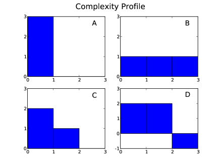
Figure 8: Complexity profile $C(k)$ for examples A through D. Note that the total (signed) area bounded by each curve equals $S(\mathfrak{D}_{\mathcal{A}})=\sum_{a\in A}H(a)=3.$

Due to the combinatorial number of dependencies for an arbitrary system, calculation of the complexity profile may be computationally prohibitive; however, computationally tractable approximations to the complexity profile have been developed baryam2012 .

VII.2 Marginal utility of information

Here we introduce an alternative measure characterizing multiscale structure: the marginal utility of information, denoted $M(y)$. This index quantifies how well a system can be characterized using a limited amount of information.

To obtain this measure, we first ask how much scale-weighted information (as defined in Section VI.3) can be represented using $y$ or fewer units of information. We call this quantity the maximal utility of information, denoted $U(y)$, and rigorously define it below. For small values of $y$, an optimal characterization will convey only large-scale features of the system. As $y$ increases, smaller-scale features will be progressively included in the description. For a given system $\mathcal{A}$, the maximal amount of scale-weighted information that can be represented, $U(y)$, is constrained not only by the information limit $y$, but also by the pattern of information overlaps in $\mathcal{A}$—that is, the structure of $\mathcal{A}$. More strongly interdependent systems allow for larger amounts of scale-weighted information to be described using the same amount of information $y$.

We define the marginal utility of information as the derivative of maximal utility: $M(y)=U^{\prime}(y)$. $M(y)$ quantifies how much scale-weighted information each additional unit of information can impart. The value of $M(y)$, being the derivative of scale-weighted information with respect to information, has units of scale.

The marginal utility of information has many properties similar to those of the complexity profile, but with the axes reversed: the argument of $M(y)$ is information, while the value of $M(y)$ has units of scale. Indeed, we show in Section IX.1 that, for a class of particularly simple systems, the marginal utility of information and the complexity profile are generalized inverses of each other. $M(y)$ declines steeply for rigid or strongly interdependent systems, and shallowly for weakly interdependent systems.

We now develop the mathematical definition of the maximal utility $U(y)$. We call any entity $d$ that imparts information about system $\mathcal{A}$ a descriptor of $\mathcal{A}$. The utility of a descriptor will be defined as a quantity of the form

$$u=\sum_{a\in A}\sigma(a)I(d;a).$$ (17)

For this to be a meaningful expression, we consider each descriptor $d$ to be an element of an augmented system $\mathcal{A}^{\dagger}=(A^{\dagger},H_{\mathcal{A}^{\dagger}})$, whose components include $d$ as well as the original components of $\mathcal{A}$, which is a subsystem of $\mathcal{A}^{\dagger}$. The amount of information that $d$ conveys about any subset $V\subset A$ of components is given by

$$\begin{split}I(d;V)&=I_{\mathcal{A}^{\dagger}}(d;V)\\ &=H_{\mathcal{A}^{\dagger}}(d)+H_{\mathcal{A}^{\dagger}}(V)-H_{\mathcal{A}^{\dagger}}\big{(}\{d\}\cup V\big{)}.\end{split}$$ (18)

For example, the amount that $d$ conveys about a component $a\in A$ can be written $I(d;a)=H(d)+H(a)-H(d,a)$. $I(d;A)$ denotes the total information $d$ imparts about the system. Because the original system $\mathcal{A}$ is a subsystem of $\mathcal{A}^{\dagger}$, the augmented information function $H_{\mathcal{A}^{\dagger}}$ coincides with $H_{\mathcal{A}}$ on subsets of $A$.

The quantities $I(d;V)$ are constrained by the structure of $\mathcal{A}$ and the laws of information theory. Applying the axioms of information functions to $H_{\mathcal{A}^{\dagger}}$, we arrive at the following constraints on $I(d;V)$:

1. $0\leq I(d;V)\leq H(V)$ for all subsets $V\subset A$.

2. For any pair of nested subsets $W\subset V\subset A$, $0\leq I(d;V)-I(d;W)\leq H(V)-H(W)$.

3. For any pair of subsets $V,W\subset A$,

   $$I(d;V)+I(d;W)-I(d;V\cup W)-I(d;V\cap W)\\ \leq H(V)+H(W)-H(V\cup W)-H(V\cap W).$$

To obtain the maximum utility of information, we interpret the values $I(d;V)$ as variables subject to the above constraints. We define $U(y)$ as the maximum value of the utility expression, Eq. (17), as $I(d;V)$ vary subject to constraints (i)–(iii) and that the total information $d$ imparts about $\mathcal{A}$ is less than or equal to $y$: $I(d;A)\leq y$.

$U(y)$ characterizes the maximal amount of scale-weighted information that could in principle be conveyed about $\mathcal{A}$ using $y$ or less units of information, taking into account the information-sharing in $\mathcal{A}$ and the fundamental constraints on how information can be shared.

$U(y)$ is well-defined since it is the maximal value of a linear function on a bounded set. Moreover, elementary results in linear programming theory wets1966 imply that $U(y)$ is piecewise linear, increasing and concave in $y$. It follows that $M(y)$ is piecewise constant, positive and nonincreasing.

The marginal utility of information satisfies four properties analogous to those satisfied by the complexity profile:

1. Conservation law: The total area under the curve $M(y)$ equals the total scale-weighted information of the system:

   $$\int_{0}^{\infty}M(y)\,dy=S(\mathfrak{D}_{\mathcal{A}}).$$ (19)

   This property follows from the observation that, since $M(y)$ is the derivative of $U(y)$, the area under this curve is equal to the maximal utility of any descriptor, which is equal to $S(\mathfrak{D}_{A})$ since utility is defined in terms of scale-weighted information.

2. Total system information: The marginal utility vanishes for information values larger than the total system information, $M(y)=0$ for $y>H(A)$, since, for higher values, the system has already been fully described.

3. Largest scale of dependency: If there are no interactions or correlations of degree $k$ or higher—formally, if $I(a_{1};\ldots;a_{k})=0$ for all collections $a_{1},\ldots,a_{k}$ of $k$ distinct components—then $M(y)\leq k$ for all $y$.

4. Additivity: If $\mathcal{A}$ separates into independent subsystems $\mathcal{B}$ and $\mathcal{C}$, then

   $$U_{\mathcal{A}}(y)=\max_{\begin{subarray}{c}y_{1}+y_{2}=y\\ y_{1},y_{2}\geq 0\end{subarray}}\left(U_{\mathcal{B}}(y_{1})+U_{\mathcal{C}}(y_{2})\right).$$ (20)

   The proof follows from recognizing that, since information can apply either to $\mathcal{B}$ or to $\mathcal{C}$ but not both, an optimal description allots some amount $y_{1}$ of information to subsystem $\mathcal{B}$, and the rest, $y_{2}=y-y_{1}$, to subsystem $\mathcal{C}$. The optimum is achieved when the total maximal utility over these two subsystems is maximized. Taking the derivative of both sides and invoking the concavity of $U$ yields a corresponding formula for the marginal utility $M$:

   $$M_{\mathcal{A}}(y)=\min_{\begin{subarray}{c}y_{1}+y_{2}=y\\ y_{1},y_{2}\geq 0\end{subarray}}\max\big{\{}M_{\mathcal{B}}(y_{1}),M_{\mathcal{C}}(y_{2})\big{\}}.$$ (21)

   Detailed proofs of Eqs. (20) and (21) are provided in Appendix E. This additivity property can also be expressed as the reflection (generalized inverse) of $M$. For any piecewise-constant, nonincreasing function $f$, we define the reflection $\tilde{f}$ as

   $$\tilde{f}(x)=\max\{y:f(y)\leq x\}.$$ (22)

   A generalized inverse baryam2012 is needed since, for piecewise constant functions, there exist $x$-values for which there is no $y$ such that $f(y)=x$. For such values, $\tilde{f}(x)$ is the largest $y$ such that $f(y)$ does not exceed $x$. This operation is a reflection about the line $f(y)=y$, and applying it twice recovers the original function. If $\mathcal{A}$ comprises independent subsystems $\mathcal{B}$ and $\mathcal{C}$, the additivity property, Eq. (21), can be written in terms of the reflection as

   $$\tilde{M}_{\mathcal{A}}(x)=\tilde{M}_{\mathcal{B}}(x)+\tilde{M}_{\mathcal{C}}(x).$$ (23)

   Eq. (23) is also proven in Appendix E.

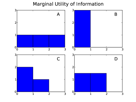
Figure 9: Marginal Utility of Information for examples A through D. The total area under each curve is $\int_{0}^{\infty}M(y)\,dy=S(\mathfrak{D})=3$. Note that in examples A, B and C, the MUI is the reflection of the complexity profile shown in Figure 8. In examples A, B and C, the MUI curves can be thought of as sums of rectangles, one rectangle for each independent subsystem.

The MUI curves for our four running examples are shown in Figure 9. Each curve is completely determined by the dependency space of that system. In each of the four examples, the conservation law Eq. (19) implies that the total area under the MUI curve is 3. We can deduce from the “largest scale of dependency” property that for example A, $M(y)\leq 1$ for all $y$. This suggests that the MUI curve for example A should be a horizontal line at $M(y)=1$ for $0\leq y<3$. We can confirm this using the additivity property, Eq. (21), because example A is a set of three independent subsystems of one component each. In example B, a set of three fully correlated components, the largest scale of dependency implies an upper bound on the MUI of $M(y)\leq 3$. We deduce that the MUI curve for example B should be $M(y)=3$ for $0\leq y<1$: describing one component describes them all, so any descriptor having an information content of 1 or more can describe the whole system. Example C can be broken down into two independent subsystems, one of a single component and the other consisting of a fully correlated pair. Providing information about the pair yields a higher return on investment, in terms of scale-weighted information, than describing the isolated component. The MUI curve of example C is thus a horizontal line $M(y)=2$ for $0\leq y<1$, which drops discontinuously to $M(y)=1$ for $1\leq y<2$, and falls to zero thereafter.

The most interesting case is the parity bit system, example D. Symmetry considerations imply that a descriptor of maximal utility conveys an equal amount of information about each of the three components $a$, $b$ and $c$. Constraints (i)–(iv) then yield that the amount described about each component must equal $y/2$ for $0\leq y\leq 2$, and 1 for $y>2$. Thus the maximal utility is $U(y)=3y/2$ for $0\leq y\leq 2$, and 3 for $y>2$, and the marginal utility of information is

$$M(y)=U^{\prime}(y)=\begin{cases}\frac{3}{2}&0\leq y\leq 2\\ 0&y>2.\end{cases}$$ (24)

More generally, if an $N$-component system has a constraint which manifests at the largest scale, and if the structure is symmetric as it is in example D, then

$$M(y)=U^{\prime}(y)=\begin{cases}\frac{N}{N-1}&0\leq y\leq N-1\\ 0&y>N-1.\end{cases}$$ (25)

A detailed derivation is provided in Appendix F.

The information overlaps among the three components of example D and the optimal descriptor with information $y$ is illustrated in Figure 10. The marginal utility of information $M(y)$ captures the intermediate level of interdependency among components in the parity bit system, in contrast to the maximal independence and maximal interdependence in examples A and B, respectively (Figure 9).

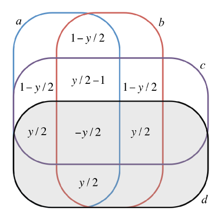
Figure 10: Information overlaps in the parity bit system, example D, augmented with a descriptor $d$ having information content $y\leq 2$ and maximal utility. The amounts of information in the region corresponding to $d$ sum to $y$, the overall information of $d$. The amounts of overlapping information among components $a$, $b$ and $c$, summing over the regions described and not described by $d$, correspond to the amounts of information overlap in the original parity bit system, which are shown in Figure 5.

The idea of descriptors provides insight into negative values of mutual information, as discussed in Section IV.2. In example D, the tertiary shared information $I(a;b;c)$ is negative. Suppose there were a descriptor $d$ which applied only to the irreducible dependency $a;b;c$ and not to any other irreducible dependency. That is, suppose $I_{\mathcal{A}_{\dagger}}(d;a;b;c)=-1$ and $I_{\mathcal{A}_{\dagger}}(d;x)=0$ for any irreducible dependency $x$ of $\mathcal{A}$ other than $a;b;c$. Then the total information in $d$, which equals the sum of $d$’s shared information with all irreducible dependencies of $\mathcal{A}$, would be negative one: $h_{\mathcal{A}_{\dagger}}(d)=-1$. This negative information is impossible according to our axioms. Thus the (negative) amount of shared information associated with the triple-overlap region cannot be described on its own. It can, however, be described implicitly as other aspects of the system are described. For instance, a complete description of the parity bit system, which contains full information about all three components ($I_{\mathcal{A}_{\dagger}}(d;a)=I_{\mathcal{A}_{\dagger}}(d;b)=I_{\mathcal{A}_{\dagger}}(d;c)=1$), implicitly contains all the information assigned to the dependency $a;b;c$. The presence of information which can only be described implicitly, rather than directly, has a physical meaning which we explore in Section X.

The MUI is closely connected to a number of other important quantities studied in different fields of science, a point we will examine in the Discussion section.

VIII Combinatorics of the Complexity Profile

Previous works have developed and applied an explicit formula for the complexity profile baryam2004a ; baryam2004b ; baryam2004c ; sgs2004 ; metzler2005 . This formula applies to the case that all components have equal intrinsic scales. To construct this formula, we first define the quantity $Q(j)$ as the sum of the joint information of all collections of $j$ components:

$$Q(j)=\sum_{i_{1},\ldots,i_{j}}H(a_{i_{1}},\ldots,a_{i_{j}}).$$ (26)

The complexity profile can then be expressed as

$$C(k)=\sum_{j=N-k}^{N-1}(-1)^{j+k-N}\binom{j}{j+k-N}Q(j+1),$$ (27)

where $N=|A|$ is the number of components in $\mathcal{A}$ baryam2004b ; baryam2004c . The coefficients in this formula can be inferred from the inclusion-exclusion principle erickson1996 . Equation (27) provides a method for computing the complexity profile for any system from the values $H(U)$ of the information function.

To relate Eq. (27) to the properties of the complexity profile discussed in Section VII.1, we consider an arbitrary system $\mathcal{A}$ of three components, $A=\{a,b,c\}$. At scale $k=1$, Eq. (27) gives

$$C(1)=Q(3)=H(a,b,c).$$ (28)

We note that $C(1)$ equals the total information in $\mathcal{A}$, consistent with Property 2 of Section VII.1. At scale 2,

$$C(2) =Q(2)-2Q(3)$$

$$=H(a,b)+H(a,c)+H(b,c)-2H(a,b,c)$$

$$=I(a;b|c)+I(a;c|b)+I(b;c|a)+I(a;b;c).$$

From the final expression above, it can be seen that $C(2)$ equals the total information in all dependencies of scale 2 or higher. We observe that this quantity vanishes if all variables are independent. Finally, for scale 3,

$$C(3) =Q(1)-Q(2)+Q(3)$$

$$=H(a)+H(b)+H(c)-H(a,b)-H(a,c)-H(b,c)+H(a,b,c)$$

$$=I(a;b;c).$$ (29)

Thus $C(3)$ returns only the information that is shared among all three variables (which may be negative, as in running example D). Again, for independent variables, $C(3)$ vanishes.

IX Special Classes of Systems

IX.1 Independent collection of intradependent blocks

One important special class of systems is those which break down into independent subsystems (“blocks”) such that all components within each block are entirely interdependent. Examples A, B and C all have this property. In example C, components $a$ and $b$ are in one block and component $c$ is in another. For such systems, the complexity profile and the marginal utility of information can both be easily computed and are related to each other in a simple manner.

In the simplest case, the entire system comprises a single block. Example B is such a system, in that the state of any one bit determines the state of all bits. More generally, for any system $\mathcal{A}=(A,H_{\mathcal{A}})$ which comprises a single block, each nonempty subset of components contains complete information about the system: $H(V)=H(A)$ for all nonempty $V\subset A$. Using the definition of the complexity profile, we find that $C(x)$ has constant value $H(A)$ for all $0\leq x\leq\sigma$ and is zero for $x>\sigma$, where $\sigma$ is the total scale of all components. We can express $C(x)$ using a step function:

$$C(x)=H(A)\Theta(\sigma-x),$$ (30)

where the $\Theta(y)$ has value 1 for $y\geq 0$ and 0 otherwise.

To compute the marginal utility of information for such a system, we observe that a descriptor with maximal utility will have $I(d;V)=\min\{y,H(A)\}$ for each subset $V\subset A$ and each value of the informational constraint $y$. From this it follows that

$$M(y)=\sigma\Theta\big{(}H(A)-y\big{)}.$$ (31)

We observe that the reflection (generalized inverse; see Section VII.2) $\tilde{M}(x)$ of $M(x)$ coincides exactly with $C(x)$.

More generally, we can consider a system which comprises $m$ independent blocks. A block is defined as a subsystem $\mathcal{B}=(B,H_{\mathcal{B}})$ with the property that $H(V)=H(B_{i})$ for each nonempty $V\subset B_{i}$. Suppose $\mathcal{A}$ is the disjoint union of blocks $\mathcal{B}_{i}=(B_{i},H_{\mathcal{B}_{i}})$ for $i=1,\ldots,m$ which are independent as subsystems (see Section V). Then additivity over independent subsystems (Property 4 in Sections VII.1 and VII.2), together with Eqs. (30) and (31), implies that

$$C(x)=\tilde{M}(x)=\sum_{i=1}^{m}H(B_{i})\Theta(\sigma_{i}-x),$$ (32)

where $\sigma_{i}$ is total scale of components in block $\mathcal{B}_{i}$.

We have thus established the following reflection principle for systems of this type:

Theorem 2.

For any system $\mathcal{A}$ composed of independent blocks, the complexity profile and the MUI are reflections of each other:

$$C(x)=\tilde{M}(x).$$ (33)

This relationship between $C(x)$ and $M(y)$ does not hold for every system. We show in Appendix F that $C(x)$ and $M(y)$ are not reflections of each other in the case of example D, and, more generally, for a class of systems that exhibit negative information.

IX.2 Systems with exchange symmetry among components

We can simplify the equations for the complexity profile for systems which have exchange symmetry—all subsets having the same number of components contain the same amount of information. Formally, for each set $U\subset A$, the information of $U$ is a function of the cardinality $|U|$, written as a subscript, $H(U)=H_{|U|}$. Examples A, B and D satisfy this constraint, but example C does not.

The monotonicity axiom, defined in Section II, implies that $H_{k}\leq H_{k+1}$. Furthermore, the strong subadditivity axiom, Eq. (1), implies that if we take the sets $U=\{a,b\}$ and $V=\{b,c\}$, then

$$H_{3}-H_{2}\leq H_{2}-H_{1}.$$ (34)

It is easy to verify that this inequality holds for examples A, B and D. For a symmetric system of $N$ components, we have the more general “concavity” property

$$H_{n+2}-H_{n+1}\leq H_{n+1}-H_{n}.$$ (35)

This follows from considering the two overlapping sets $U=\{a_{1},\ldots,a_{n},a_{n+1}\}$ and $V=\{a_{2},\ldots,a_{n},a_{n+1},a_{n+2}\}$. The symmetry condition lets us write $H(U)=H(V)=H_{n+1}$, while the information of their union is $H(U\cup V)=H_{n+2}$ and that of their intersection is $H(U\cap V)=H_{n}$. From this concavity property, it follows that if $H_{j+1}=H_{j}$ for some $j$, then $H_{k}=H_{j}$ for all $k\in\{j,\ldots,N\}$; that is, once the information levels off, it stays level.

Concavity is easy to verify if $H_{j}$ is constant, the case of complete interdependence; or if $H_{j}$ is proportional to $j$, the case of complete independence. It also is manifest in the more general situation $H_{j}\propto j^{\alpha}$, where the “independence parameter” $\alpha$ interpolates from $\alpha=0$ (interdependence) to $\alpha=1$ (independence).

Exchange symmetry also simplifies the form of the complexity profile. The result takes a particularly appealing form when stated in terms of the information in dependencies of scale $k$ and no higher, which we denote $D(k)$. Recalling that the complexity profile $C(k)$ indicates the information in dependencies of scale $k$ and higher, we write

$$D(k)=C(k)-C(k+1).$$ (36)

The sum of $D(k)$ over all scales $k$ is $C(1)$. As we did for $C(k)$, we can write a combinatorial formula for $D(k)$:

$$D(k)=\sum_{j=N-k}^{N}(-1)^{j+k-N+1}\binom{j}{j+k-N}Q(j).$$ (37)

When exchange symmetry holds, the information specific to scale $k$ becomes

$$D(k)=\binom{N}{k}\sum_{l=0}^{k}(-1)^{l+1}\binom{k}{l}H_{l+N-k},$$ (38)

while the information of scale $k$ and higher becomes

$$C(k)=\binom{N}{k}(-1)^{k}\sum_{l=0}^{k-1}(-1)^{l+1}\frac{k-l}{l+N-k+1}\binom{k}{l}H_{l+N-k+1}.$$ (39)

For any fixed scale $k$, the complexity $D(k)$ is (up to a prefactor) the binomial transform of the sequence $a_{l}\equiv H_{l+N-k}$. This, combined with the concavity property, allows one to confirm that $D(k)\geq 0$ for $k=1,2$; i.e., complexity can only be negative at scale $k=3$ or higher. Negative $D(k)$ arises from the leveling-off of the information content $H_{j}$.

The binomial transform of a sequence can be rewritten using the forward difference operator, $\Delta$, whose action on a sequence $\{a_{n}\}$ is given by $(\Delta a)_{n}=a_{n+1}-a_{n}$. The complexity $D(k)$ is given by the $k$^th finite difference of $H_{l+N-k}$:

$$D(k)=\binom{N}{k}(-1)^{k}(\Delta^{k}H_{N-k})_{0}.$$ (40)

Exchange symmetry among components is a reasonable and useful simplification for some physical systems. We discuss its relevance to kinetic theory in Appendix G. Previous work studied the complexity profile of the Ising model in the case of exchange symmetry sgs2004 .

IX.3 Weakly Interdependent Systems

Suppose that the components of our system are only weakly coupled, as would be the case in a nearly-ideal gas or a magnet at high temperature. Then the complexity profile $C(k)$ will be rapidly decaying, similar to example A, and the total scale-weighted information of the dependency space, $S(\mathfrak{D})$, will be roughly given by the first-scale complexity $C(1)$. For some purposes, $C(1)$ is what we wish to obtain: for a physical system in thermal equilibrium, $C(1)$ is the physical entropy, which connects statistics to thermodynamics. We now derive approximations for $S(\mathfrak{D})$ and for $C(1)$ which are useful in the weak-coupling limit.

From the conservation-law property of the complexity profile, Eq. (16), we know that the total scale-weighted information $S(\mathfrak{D})$ is the sum of $C(k)$ over all scales $k$. Progressively improved approximations can be obtained by taking partial sums of the form

$$S(\mathfrak{D})\approx\sum_{k=1}^{k_{\mathrm{max}}}C(k),$$ (41)

where $1\leq k_{\mathrm{max}}\leq|A|$ is the degree of the approximation. This method is applicable when dependencies at larger scales—binary, tertiary and so forth—become less significant even as their number increases combinatorially. The approach relies on neglecting shared information at scales greater than a cutoff $k_{\mathrm{max}}$, i.e., large-scale dependencies among the system components. In some circumstances, this approximation can characterize the system behavior.

We now develop a systematic approach for approximating $C(1)$ given quantities of shared information pertaining to progressively larger scales. For the first-order approximation, we neglect all shared information pertaining to scales greater than 1, yielding

$$C(1)\approx S(\mathfrak{D})=\sum_{i=1}^{|A|}H(a_{i}).$$ (42)

This is the first-order approximation according to Eq. (41). We refine this approximation using the inclusion-exclusion principle applied to the dependency space. If information is shared among pairs of components, the first-order estimate of $C(1)$ is too large. We subtract from it the shared information within pairwise dependencies.

$$C(1)\approx\sum_{i=1}^{|A|}H(a_{i})-\sum_{i\neq j}I(a_{i};a_{j}).$$ (43)

This, in turn, undercounts the shared information content of tertiary dependencies, so we add the tertiary mutual information summed over all triplets, and so on. Continuing this process, we write the entropy $C(1)$ as the sum

$$C(1)=\sum_{i=1}^{|A|}H(a_{i})-\sum_{i\neq j}I(a_{i};a_{j})+\sum_{i\neq j\neq k}I(a_{i};a_{j};a_{k})-\ldots$$ (44)

Truncating this series after $k_{\mathrm{max}}$ terms, where $1\leq k_{\mathrm{max}}\leq|A|$, constitutes an approximation of the entropy $C(1)$ to order $k_{\mathrm{max}}$.

If the system has exchange symmetry as discussed in the previous section, then the shared information of any dependency including $k$ components is

$$I_{k}\equiv\sum_{l=1}^{k}(-1)^{l+1}\binom{k}{l}H_{l}.$$ (45)

With this relation, Eq. (44) for the joint entropy simplifies to

$$C(1)=\sum_{k=1}^{|A|}(-1)^{k+1}\binom{|A|}{k}I_{k}.$$ (46)

The complete sum yields the exact value of $C(1)$, which is the joint information of all components, $H_{|A|}$. Indeed, if one performs the entire sum over all scales, everything cancels except $H_{|A|}$, because the binomial transform from $\{H_{l}\}$ to $\{I_{k}\}$ is its own inverse.

One field where this approximation is valuable is the kinetic theory of fluids green1952 . Here, one is interested in approximating the entropy $C(1)$ as well as possible given only small-scale correlations. Green’s expansion is a method for doing this systematically. The terms in Green’s expansion are integrals over probability distributions involving successively larger numbers of variables (see Appendix G). However, the motivation for each term, and the derivation of the coefficients, is not straightforward. The meaning of Green’s expansion becomes clear when the expansion is interpreted using Shannon information theory and our multiscale formalism. Green’s expansion is Eq. (46), written in the language of kinetic theory. Furthermore, all the coefficients in Green’s entropy expansion follow from the fact that the binomial transform is self-inverse. This is one example of the valuable perspective gained by starting with a general axiomatic framework.

X Multiscale Cybernetic Thermodynamics

Thus far, we have considered system structure as an unchanging quantity, and without explicit interaction of the system with its environment. We now build on this conceptual foundation by studying systems influenced by their surroundings. We consider the problem of intentional influences, which an agent outside a system uses to regulate, guide or exploit that system. Our approach enables us to consider one of the primary limitations which intentional agents often face. Typically, an agent has only partial information about a system of interest. Furthermore, the available information may pertain to a limited set of scales. Our multiscale formalism allows us to express the limitations which an agent faces in such a situation.

We consider, as a simple but illustrative example, the Szilárd engine, a gedankenexperiment consisting of a cylinder immersed in a heat bath bennett1982 ; feynman1996 ; delrio2010 ; toyabe2010 ; koski2014 ; jun2014 . Each end of the cylinder (left and right) is a moveable piston. In the middle of the cylinder is a partition separating the left and right halves which can be removed and reinserted, and somewhere within the cylinder, on one side or the other of the partition, is a single atom. When the Szilárd engine is in thermal equilibrium with the surrounding heat bath, we can extract useful work from it, provided we know which side of the partition the atom is on.

The operational cycle of the Szilárd engine extracts energy from information. The engine operator (engineer) uses one bit of knowledge about the atom’s location, which side of the partition it is on, to extract an energy $k_{B}T\log 2$. After the operation, the atom is equally likely to be on either side of the partition, so further cycling requires gaining new knowledge about the engine’s internal configuration (and, if the engineer has a finite memory, therefore requires erasing the prior datum within that memory feynman1996 ). An engineer who has no knowledge of the atom’s position inside the Szilárd cylinder is just as likely to expend energy working the machine as they are to extract it, so on average, they will obtain no useful work from the device.

The process of energy extraction from information starts with the partition in place and engineer knowledge of which side of the partition the atom is on. If the atom is on the left side of the partition, the engineer pushes the piston in from the right-hand side without expending energy. The engineer removes the partition and the bouncing atom pushes the cylinder back as heat flows into the cylinder from the reservoir. The heat flow keeps the atom at the same average kinetic energy despite pushing the cylinder. After the piston reaches the right-hand end of the cylinder, the engineer re-inserts the partition. At this time, the atom can be anywhere within the cylinder. The magnitude of the energy obtained $k_{B}T\log 2$ is set by the thermal energy of the heat bath, $k_{B}T$. The factor of $\log 2$ originates from the change in the spatial volume accessible to the atom during the Szilárd engine cycle, which doubles. A doubling in volume is associated with an increase of thermodynamic entropy given by

$$\Delta S=k_{B}\log\left(\frac{V_{\rm final}}{V_{\rm initial}}\right)=k_{B}\log 2.$$ (47)

The information resource required to operate a Szilárd engine is more properly expressed as a mutual information between the engine and its engineer (or control mechanism). Consider an engineer presented with an ensemble of $L$ Szilárd cylinders. If the configuration of each cylinder is predictable, then the engineer can extract $Lk_{B}T\log 2$ of energy by the end of the sequence. If the configurations are completely uncertain, the expected energy gain averages to zero. More generally, the energy gain decreases by $k_{B}T\log 2$ for each cylinder for which the engineer must ask, “Is the atom on the left side of the partition?” Thus, the amount of energy which the engineer can extract from this sequence is $(L-H)k_{B}T\log 2$, where $H$ is the number of yes/no questions which the engineer must ask about the sequence bennett1982 ; feynman1996 . The number of yes/no questions about $X$ which one can answer knowing the value of $Y$ is their mutual information. If the engineer has access to a variable $Y$ which provides partial information about the configuration of the cylinder sequence, then $H$ is reduced by the mutual information between $Y$ and the cylinders, and the energy gain increases proportionally. Since this is true for an ensemble of independent cylinders, for each cylinder in the ensemble the expected energy gain is proportional to the available information about that cylinder.

We can also consider multiple Szilárd cylinders as a single system, which leads to a multiscale generalization. Imagine $N$ Szilárd cylinders immersed in a heat bath at temperature $T$. The relevant property of each cylinder, the side occupied by an atom, is a random variable. Knowing about the positions of the atoms inside the cylinders—that is, having a description of the $N$ system components—allows an engineer to extract energy, at the cost of making obsolete that knowledge. Correlations among cylinders imply that knowledge applicable to one is also applicable to another, so that knowledge of one cylinder can be leveraged for a greater energy gain.

When we characterize the configuration of a multi-cylinder Szilárd engine, a natural measure of the usefulness of a descriptor is the amount of energy we can extract from the machine using that descriptor. Here, the benefit of having a formalism that characterizes the mutual information between the observer and the system becomes apparent. The available energy is proportional to the utility defined in Section VII.2. The descriptor $d$ has a mutual information $I(d;X_{i})$ with the $i$^th cylinder of the engine. Having this much information about cylinder $X_{i}$ enables extracting from $X_{i}$ a quantity of energy proportional to the mutual information and to the thermal energy $k_{B}T$. (Sagawa and Uedo Sagawa2012 provide an explicit protocol for extracting the energy $k_{B}TI(d;X)\log 2$ in the case where the descriptor $d$ provides accurate knowledge of the cylinder $X$ with some error rate, $\epsilon$. The key step of the protocol is to only move the piston partway, due to the probability of error.)

The MUI measures the amount of additional energy which can be gained by making use of additional information. Given the ability to choose information that one knows about the system, the additional energy that can be gained is $\Delta E=M(y)k_{B}T\log 2$.

A real-world engineer working with ordinary tools can possess only coarse-grained information about a system. Therefore, what the engineer can do with that system is limited. Classical thermodynamics is a phenomenological macroscopic treatment of this situation. The other extreme is the hypothetical being known as Maxwell’s Demon, which has exhaustive information about the finest-scale details of the system. The demon can exploit this information to extract the maximal possible energy. Descriptions having partial utility realize the “continuum of positions” fuchs2012inbook between these two extremes.

We can use our indices of multiscale structure to characterize what an intentional agent can do when equipped with information that applies to particular scales. A single bit that is relevant at a large scale provides the opportunity to extract a large amount of energy. For example, given $k$ dependent cylinders, we can extract in total $k\times k_{B}T\log 2$ units of energy by acting independently on each cylinder. There are subtleties, however, in the macroscopic process of extracting this energy. If the information that is available indicates that all cylinders are in the same state, a single coherent action may be used to extract all the energy. If the cylinders are specified to alternate in some spatially structured way, the ability to extract the energy using a coherent action requires a mechanism to couple to that alternating structure.

More generally, we can consider engines that comprise independent blocks of cylinders. A multi-cylinder Szilárd engine of this type is a system in which all components have the same intrinsic scale and one bit of information apiece: $\sigma(a)=\sigma$, $H(a)=1$ for all $a\in A$. Then $D(k)$, as defined in Eq. (36), is the number of blocks of size $k$. Knowing the internal configuration of each block requires one bit of information and enables the extraction of $(k_{B}T)k\log 2$ in energy. One block is not correlated with another, so making use of a second block requires a second bit of data. In all, making use of all blocks at scale $k$ requires $D(k)$ bits and results in an energy gain $E$ given by

$$\frac{E}{k_{B}T}=D(k)k\log 2.$$ (48)

We recall that generally the sum of $D(k)$ over all scales $k$ is $C(1)$, which in this context is the joint Shannon information for the entire multi-cylinder Szilárd engine. Therefore, $C(1)$ is the amount of information required in order to extract the energy from all the blocks.

For any multi-cylinder Szilárd engine, even one not made of independent blocks, if we have $C(1)$ bits of information, we can predict the configuration of all the cylinders. We can, therefore, extract the maximum total amount of energy, by operating on each cylinder in turn. However, it is not generally true that $D(k)$ represents an extractable amount of energy for each value of $k$, even though summing $D(k)$ over all $k$ always yields $C(1)$. If $D(k)$ is negative for some scale $k$, as in example D, then there exists no partial description which allows the Szilárd engine operator to extract the energy associated with scale $k$ and no other. Information which can only be specified implicitly cannot be utilized in isolation, only as part of an operation on a larger dependency within a system.

XI Discussion

XI.1 Characterizing complex systems

Let us return to the question posed in the Introduction of how a complex system can be quantitatively defined. Of all systems of $n$ components, with fixed values $H(a_{1}),\ldots,H(a_{n})$ for the information of individual components, which can be characterized as “complex” and what constitutes an appropriate measure of complexity? The maximal total information $H(A)$ is achieved by letting all components be independent, so that $H(A)=H(a_{1})+\ldots+H(a_{n})$. However, such a system contains no nontrivial interactions or dependencies, and is thus rather simple from a complex systems point of view.

Our formalism resolves this difficulty by emphasizing that all information applies at a particular scale. In a system of fully independent components, information is maximized at the lowest scale but is absent at any higher scale. In contrast, the systems of greatest interest to complex systems researchers contain information at many scales, with larger-scale information arising from redundancy in smaller-scale information. This key property of complex systems is captured in our two indices of structure, the complexity profile and the marginal utility of information. Both indices quantify the amount of information that applies at each scale, allowing the systems that exhibit multiscale complexity to be identified.

To illustrate this point, consider the example mentioned in the Introduction of a box containing both a crystal and an ideal gas. For this system, information applies at two scales: that of the crystal and that of the gas particles. The complexity profile for the contents of the box is the sum of two rectangles (i.e., step functions), one indicating the large-scale structure of the crystal and the other the small-scale structure of the ideal gas. By the reflection principle, the MUI curve for this joint system is also the sum of two rectangles. Both indices of structure make clear that the gas-and-crystal example lacks the multiscale organization that distinguishes complex systems.

All systems are subject to a tradeoff in independence versus interdependence, due to the fact that larger-scale information arises from overlaps in the information pertaining to indvidual components. This tradeoff is captured in our formalism by the conservation of the total scale-weighted information $S(\mathfrak{D}_{\mathcal{A}})$ (Theorem 1). Both the complexity profile and the MUI reflect this tradeoff in their respective conservation laws, Eqs. (16) and (19).

XI.2 Negentropy

The idea of using entropy or information to quantify structure has deep roots in physics. One of the earliest and most influential attempts was Schrödinger’s concept of negative entropy schrodinger1944life , later shortened to negentropy brillouin1953negentropy , defined as the difference between a system’s actual entropy and the maximum possible entropy of a system with the same matter, energy and volume. Schrödinger introduced negentropy to express the quality of order in living organisms due to their nonequilibrium nature. Living beings are not in a state of maximum possible entropy, and negentropy is an attempt to quantify this difference. We consider this attempt to be limited, in that it does not capture the multiscale aspect of organization present in living systems.

To make this point clear, we first define negentropy exactly within our information-theoretic framework. Consider a physical system $\mathcal{A}$ in which the information of a subset of components is defined as the joint physical entropy of these components considered together. For convenience, assume each component has unit scale. The maximum possible entropy of such a system—which would be attained if all components of $\mathcal{A}$ were independent—is equal by Theorem 1 to the total scale-weighted information $S(\mathfrak{D}_{\mathcal{A}})$. In contrast, the actual entropy of $\mathcal{A}$ is equal to the total (non-scale-weighted) information $I(\mathfrak{D}_{\mathcal{A}})$, which can also be identified as $C(1)$. The negentropy (i.e., the difference between the maximum possible and actual entropy) can thus be defined as $J(\mathcal{A})=S(\mathfrak{D}_{\mathcal{A}})-I(\mathfrak{D}_{\mathcal{A}})$. We remark that negentropy is equivalent to the quantity called “multi-information” in network information theory studeny1998multiinformation ; schneidman2003network ; kolchinsky2011 . Since we have assumed that all components have scale one, the total information, $I(\mathfrak{D}_{\mathcal{A}})$, equals the information at scale one, $C(1)$. We can then use the conservation law, Eq. (16), to express negentropy in terms of the complexity profile:

$$J(\mathcal{A})=\sum_{k=1}^{\infty}C(k)-C(1)=\sum_{k=2}^{\infty}C(k).$$ (49)

Negentropy represents a limited view of organization in that it treats as the same all scales but the smallest. According to this measure, it is irrelevant whether a decrease of entropy arises from many bits at scale 2 or a few bits at much larger scale. This can be seen from examples C and D, which both have negentropy equal to one bit, despite having qualitatively different kinds of structure. The importance of the specific scale of the structure is captured by our indices that include scale as a complementary axis to information. Given the significance of macroscopic structure to scientific observations of physical, biological and social systems, it seems that a useful measure must necessarily make this distinction.

XI.3 Requisite variety

The discipline of cybernetics, an ancestor to modern control theory, used Shannon’s information theory to quantify the difficulty of performing tasks, a topic of relevance both to organismal survival in biology and to system regulation in engineering. Cyberneticist W. Ross Ashby considered scenarios in which a regulator device must protect some important entity from the outside environment and its disruptive influences ashby1956 . In Ashby’s examples, each state of the environment must be matched by a state of the regulatory system in order for it to be able to counter the environment’s influence on a protected component. Successful regulation implies that if one knows only the state of the protected component, one cannot deduce the environmental influences; i.e., the job of the regulator is to minimize mutual information between the protected component and the environment. This is an information-theoretic statement of the idea of homeostasis. Ashby’s “Law of Requisite Variety” states that the regulator’s effectiveness is limited by its own information content, or variety in cybernetic terminology. An insufficiently flexible regulator will not be able to cope with the environmental variability. A multiscale extension of Shannon information theory provides a multiscale cybernetics, with which we can study the scenarios in which “that which we wish to protect” and “that which we must guard against” are each systems of many components, as are the tools we employ for regulation and control baryam2004a ; baryam2004b ; baryam2004c .

Multiscale information theory enables us to overcome a key limitation of the requisite variety concept. In the examples of traditional cybernetics ashby1956 , each action of the environment requires a specific, unique reaction on the part of the regulator. This neglects the fact that the impact which an event in the environment has on the system depends upon the scale of the environmental degrees of freedom involved. There is a great difference between large-scale and fine-scale impacts. Systems can deflect fine-scale impacts without needing to specifically respond to them, while they need to respond to large-scale ones or perish. For example, a human being can be indifferent to the impact of a falling raindrop, whereas the impact of a falling rock is much more difficult to neglect, even if specifying the state of the raindrop and the state of the rock require the same amount of information. An extreme case is the impact of a molecule: air molecules are continually colliding with us, yet the only effects we have to cope with actively are the large-scale, collective behaviors like high-speed winds. Ashby’s Law does not make this distinction. Indeed, there is no framework for the discussion due to the absence of a concept of scale in the information theory he used: Each state is equally different from every other state and actions must be made differently for each different environment.

Thus, in order to account for the real-world conditions, a multiscale generalization of Ashby’s Law is needed. According to such a Law, the responses of the system must occur at a scale appropriate to the environmental change, with larger-scale environmental changes being met by larger-scale responses. As with the case of raindrops colliding with a surface, large-scale structures of a system can avoid responding dynamically to small-scale environmental changes which cause only small-scale fluctuations in the system.

Given a need to respond to larger-scale changes of the environment, coarser-scale descriptions of that environment may suffice. A regulator that can marshall a large-scale response can use a coarse-grained description of the environment to counteract large-scale fluctuations in the external conditions. In this way, limited amounts of information can still be useful. To make requisite variety a practical principle, one must recognize that information applies to specific scales.

Ashby aimed to apply the requisite variety concept to biological systems, as well as technological ones. An organism which lacks the flexibility to cope with variations in its environment dies. Thus, a mismatch in variety/complexity is costly in the struggle for survival, and so we expect that natural selection will lead to organisms whose complexity matches that of their environment. However, “the environment” of a living being includes other organisms, both of the same species and of others. Organisms can act and react in concert with their conspecifics, and the effect of any action taken can depend on what other organisms are doing at the same time allen2014 . In some species, such as social insects tschinkel2014 , distinct scales of the individual, colony and species are key features characterizing collective action. This suggests a multiscale cybernetics approach to the evolution of social behavior: We expect that scales of organization within a population—the scales, for example, of groups or colonies—will evolve to match the scales of the challenges which the environment presents. Furthermore, the concept of multiscale response applies within the individual organism as well. Multiple scales of environmental challenges are met by different scales of system responses. To protect against infection, for example, organisms have physical barriers (e.g., skin), generic physiological responses (e.g., clotting, inflammation) and highly specific adaptive immune responses, involving interactions among many cell types, evolved to identify pathogens at the molecular level. The evolution of immune systems is the evolution of separate large- and small-scale countermeasures to threats, enabled by biological mechanisms for information transmission and preservation stacey2008 . As another example, the muscular system includes both large and small muscles, comprising different numbers of cells, corresponding to different scales of environmental challenge (e.g.,  pursuing prey and escaping from predators versus chewing food) bar2003complexity .

XI.4 Benefits of an axiomatic formalism

Because complex systems arise in a wide range of scientific contexts, it is challenging to formulate consistent definitions for key concepts. Rooting our definitions in mathematically general axioms for information enables our formalism to apply to a wide range of empirical and model systems.

The axiomatic basis of our constructions also allows the unification of ideas from different areas of mathematics and science. For example, the definition of independence in Eq. (10)—which subsumes the definitions of independent random variables and of linearly independent vector spaces—allows the notion of independence to be applied rigorously in any context for which an information function is available. A further example is conditional independence, which is defined in probability theory in terms of the joint distribution of three or more random variables. This definition implies a condition on the Shannon entropies of the distributions involved, a condition which can be abstracted to a more general information measure context. Specifically, system components $a_{1}$ and $a_{3}$ are conditionally independent given component $a_{2}$ if

$$H(a_{1},a_{3}|a_{2})=H(a_{1}|a_{2})+H(a_{3}|a_{2}).$$ (50)

This enables discussions of Markov chains, Markov random fields steudel2010 and “computational mechanics” ellison2009 ; mahoney2009 ; crutchfield2009 ; crutchfield2011 to be subsumed in a general formalism and thence applied in algorithmic, vector-spatial or matroidal contexts.

XI.5 Approximations to the marginal utility of information

Our new index of structure, the MUI, is philosophically similar to data-reduction or dimensional reduction techniques like principal component analysis, multidimensional scaling and detrended fluctuation analysis peng1994 ; hu2002 ; to the Information Bottleneck methods of Shannon information theory slonim1999 ; shalizi2000 ; tishby2000 ; ziv2005 ; to Kolmogorov structure functions and algorithmic statistics in Turing-machine-based complexity theory vereshchagin2003 ; gruenwald2004 ; vitanyi2006 ; and to Gell-Mann and Lloyd’s “effective complexity” gellmann1996infomeasures . All of these methods are mathematical techniques for characterizing the most important behaviors of the system under study. Each is an implementation of the idea of finding the best possible brief description of a system, where description length is measured in bits or by the number of coordinates employed. However, MUI can be formulated completely generally, in terms of our basic postulates for information functions. Furthermore, the MUI is by definition the optimal such characterization.

We have defined MUI in terms of optimally effective descriptors: for each possible amount of information invested in describing the system, we use the descriptor which provides the best possible theoretical return (in terms of scale-weighted information) on that investment. However, in applied contexts, it may be difficult or impossible to realize these theoretical maxima, due to constraints beyond those imposed by the axioms of information functions. It is often useful in these contexts to consider a particular “description scheme”, in which descriptors are restricted to be of a particular form. In this case, the maximal utility we find following that description scheme can be less than the theoretical maximal utility defined by the system’s dependency space. We would in such a case find an approximation to the MUI, rather than the MUI itself.

We can illustrate this issue with a straightforward description scheme: using subsets of the system’s component set as descriptors. In this scheme, a descriptor $d$ is a set drawn from the set of all components $A$, and the length of a descriptor is just the number of components used in it. Any descriptor $d$ naturally provides the full quantity of information about the components from $A$ which are included in $d$ itself. If correlations exist among the system’s components, then the elements of $d$ also provide information about other components of the system. The maximal utility possible within this description scheme at a given descriptor length $x$ is given by maximizing $\sum_{a\in A}I(d;a)$ over all possible choices of descriptor $d$ which have length $x$. The finite difference of this utility curve is an approximation to the MUI. It is not difficult to see that for examples A, B and C this approximate MUI is the same as the ideal MUI. For example D, however, the approximation and the ideal differ. Because the components in example D are pairwise independent, any one-component descriptor only describes the component it mirrors, so the maximal utility approximation at length 1 is 1. A descriptor using two components can describe the whole system, so the maximal utility approximation at length 2 is 3. Therefore, the approximated MUI in the confines of this description scheme is a nonmonotonic function of descriptor length, starting at 1 and rising to 2 before falling back to 0. This nonmonotonicity is a consequence of the negative information in example D’s dependency space.

Other choices of description scheme are also possible. These description schemes bring other, more familiar quantities into the information-theoretic framework. Within an algorithmic context, for example, one might study the increasing utility of algorithmic descriptions as a function of the computational resources available.

XI.6 Mechanistic versus informational dependencies

Our indices of structure measure multi-component relationships, including statistical correlations among random variables. A key question is how causal interactions give rise to such relationships. Importantly, causal influences at one scale can produce correlations at another. For example, the interactions in an Ising spin system are pairwise in character: the interaction energy of a pair of spins is not affected by other spins being up or down elsewhere in the lattice. These pairwise couplings can, however, give rise to long-range patterns kardar2007 . Similarly, in commonly-used models of coupled oscillators, the effect one oscillator has on another—the force with which component $i$ pulls on component $j$—depends only on the relative phase difference between those two oscillators, and the total influence on an oscillator due to all the others with which it is coupled is just the sum of their influences. Yet, even though the forces are dyadic, synchronization among oscillators creates collective, coherent behavior dorogovtsev2010 . Synchronization, in other words, creates structure on a large scale.

XI.7 Limitations of network representations

Representing system structure by networks, a common practice in the complex-systems field, prioritizes pairwise (scale two) relationships and may neglect higher-scale dependencies. Often, a network model is formulated by computing a measure of correlation for each pair of components, and drawing an edge between the corresponding vertices if that correlation is statistically significant dorogovtsev2010 ; harmon2010 . This procedure discards information at scales three and higher.

One way to incorporate higher-scale information into a network representation is by changing what the presence of an edge means. For an illustrative example, take the case of gene regulation, in which the system components are genes and a joint probability distribution describes their expression levels. We expect that if the expression level of one gene predicts the that of another, this relationship may be biologically significant. We could make a straightforward network depiction by linking the vertices corresponding to genes $a_{i}$ and $a_{j}$ if their mutual information is large. However, not all of these edges will represent direct paths of biochemical influence. Suppose that gene $a_{1}$ boosts the expression of gene $a_{2}$, which in turn boosts the expression of gene $a_{3}$. In this case, the measured mutual information of each of the three pairs $(a_{1},a_{2})$, $(a_{1},a_{3})$ and $(a_{2},a_{3})$ could be large, even though there is no direct causal link between $a_{1}$ and $a_{3}$. To distinuguish between direct and indirect relationships, one must test for the conditional independence of components that are correlated at the pairwise level. This analysis requires information on three-fold and higher correlations. Bayesian networks friedman2000using are one way of incorporating such higher-order correlations into a network model.

In contrast, our framework incorporates multiscale information not as a tool for refining pairwise relationships, but as an important aspect of structure in its own right. Such multiscale information can arise from pairwise mechanisms (as discussed above), or from causal relationships that are intrinsically of scale three or higher. For example, suppose the expression levels of three genes jointly satisfy a nonlinear constraint due to joint reliance on a common precursor or other resource. Such a relationship may not be representable within a Bayesian network, but can be represented in terms of information shared among these genes.

XII Conclusion

Over the past century, science has made enormous strides in understanding the fundamental building blocks of physics and biology. However, it is increasingly clear that understanding the behaviors of physical, biological and social systems requires more than a characterization of their constituent parts. Rather, scientific progress depends on a theory of system structure. While many conceptual elements of such a theory have been developed within the field of complex systems, a general quantitative framework has so far been elusive.

Our work aims to provide a mathematical foundation for complex systems theory, in which the fundamental concepts of dependence, scale and structure are given precise meaning. This is achieved via an axiomatic formalism for information that generalizes classical information theory. This formalism enables us to identify structure as the sharing of information among system components. A system’s structure can be summarized by its complexity profile or its MUI function, both of which highlight the scale of system behaviors.

Already, we have found that our framework resolves key conceptual puzzles, from the combinatorial origins of kinetic-theory expressions to the characterization of “complex systems.” We hope this mathematical formalism of structure can aid in the scientific transition from understanding the components of systems to understanding systems themselves.

Appendix A Total scale-weighted information

Here we prove Theorem 1 of the main text, which we restate here for convenience:

Theorem 1.

For any system $\mathcal{A}$, the total scale-weighted information, $S(\mathfrak{D}_{\mathcal{A}})=\sum_{x\in\mathfrak{D}_{\mathcal{A}}}s(x)I(x)$, is given by the scale and information of each component, independent of the information shared among them:

$$S(\mathfrak{D}_{\mathcal{A}})=\sum_{a\in A}\sigma(a)H(a).$$ (51)

Proof.

The proof amounts to a rearrangement of summations. We begin with the definition of scale-weighted information,

$$S(\mathfrak{D}_{\mathcal{A}})=\sum_{x\in\mathfrak{D}_{\mathcal{A}}}s(x)I(x).$$ (52)

Substituting the definition of $s(x)$ (main text, 11) and rearranging yields

$$S(\mathfrak{D}_{\mathcal{A}}) =\sum_{x\in\mathfrak{D}_{\mathcal{A}}}\left(\sum_{\begin{subarray}{c}a\in A\\ x\text{ includes }a\end{subarray}}\sigma(a)\right)I(x)$$

$$=\sum_{a\in A}\sigma(a)\sum_{\begin{subarray}{c}x\in\mathfrak{D}_{\mathcal{A}}\\ x\text{ includes }a\end{subarray}}I(x)$$

$$=\sum_{a\in A}\sigma(a)I(\delta_{a})$$

$$=\sum_{a\in A}\sigma(a)H(a).\qed$$

Appendix B Conservation Law for the Complexity Profile

In this Appendix, we prove the conservation law for the complexity profile, Eq. (16) of the main text. We state this law as follows:

Theorem 3.

The area under the complexity profile of a system $\mathcal{A}$ is equal to the total scale-weighted information of $\mathcal{A}$:

$$\int_{0}^{\infty}C(y)\;dy=S(\mathfrak{D}_{\mathcal{A}}).$$ (53)

Proof.

We begin by substituting the definition of $C(y)$:

$$\int_{0}^{\infty}C(y)\;dy =\int_{0}^{\infty}I\big{(}\{x\in\mathfrak{D}_{\mathcal{A}}\;:\;\sigma(x)\geq y\}\big{)}\;dy$$

$$=\int_{0}^{\infty}\left(\sum_{\begin{subarray}{c}x\in\mathfrak{D}_{\mathcal{A}}\\ y\leq\sigma(x)\end{subarray}}I(x)\right)dy.$$

We then interchange the sum and integral on the right-hand side and apply Theorem 1:

$$\int_{0}^{\infty}C(y)\;dy =\sum_{x\in\mathfrak{D}_{\mathcal{A}}}\left(I(x)\int_{0}^{\sigma(x)}\;dy\right)$$

$$=\sum_{x\in\mathfrak{D}_{\mathcal{A}}}\sigma(x)I(x)$$

$$=S(\mathfrak{D}_{\mathcal{A}}).\qed$$

Appendix C Properties of Independent Subsystems

Here we prove fundamental propeties of independent subsystems, which will be used to prove the additivity property of the complexity profile. Our first target is the hereditary property of independence (Theorem 5), which asserts that subsystems of independent subsystems are independent perfect1981independence . We then establish in Theorem 8 a simple characterization of information in systems composed of independent subsystems.

For $i=1,\ldots,k$, let $\mathcal{A}_{i}=(A_{i},H_{\mathcal{A}_{i}})$ be subsystems of $\mathcal{A}=(A,H_{\mathcal{A}})$, with the subsets $A_{i}\subset A$ disjoint from each other. We recall the information-theoretic definition of independent subsystems from Section V.

Definition 1.

The subsystems $\mathcal{A}_{i}=(A_{i},H_{\mathcal{A}_{i}})$ are independent if

$$H(A_{1}\cup\ldots\cup A_{k})=H(A_{1})+\ldots+H(A_{k}).$$

We establish the hereditary property of independence first in the case of two subsystems (Lemma 4), using repeated application of the strong subadditivity axiom. We then extend this result in Theorem 5 to arbitrary numbers of subsystems.

Lemma 4.

If $\mathcal{A}_{1}$ and $\mathcal{A}_{2}$ are independent subsystems of $\mathcal{A}$, then for every pair of subsets $U_{1}\subset A_{1}$, $U_{2}\subset A_{2}$, $H(U_{1}\cup U_{2})=H(U_{1})+H(U_{2})$.

Proof.

The strong subadditivity axiom, applied to the sets $A_{1}$ and $U_{1}\cup A_{2}$, yields

$$H(A_{1}\cup A_{2})\leq H(A_{1})+H(U_{1}\cup A_{2})-H(U_{1}).$$

Replacing the left-hand side by $H(A_{1})+H(A_{2})$ and adding $H(U_{1})-H(A_{1})$ to both sides yields

$$H(U_{1})+H(A_{2})\leq H(U_{1}\cup A_{2}).$$ (54)

Now applying strong subadditivity to the sets $U_{1}\cup U_{2}$ and $A_{2}$ yields

$$H(U_{1}\cup A_{2})\leq H(U_{1}\cup U_{2})+H(A_{2})-H(U_{2}).$$

Combining with (54) via transitivity, we have

$$H(U_{1})+H(A_{2})\leq H(U_{1}\cup U_{2})+H(A_{2})-H(U_{2}).$$

Adding $H(U_{2})-H(A_{2})$ to both sides yields

$$H(U_{1})+H(U_{2})\leq H(U_{1}\cup U_{2}).$$ (55)

But strong subadditivity applied to $U_{1}$ and $U_{2}$ yields

$$H(U_{1}\cup U_{2})\leq H(U_{1})+H(U_{2})-H(U_{1}\cap U_{2})\leq H(U_{1})+H(U_{2}).$$ (56)

We conclude from inequalities (55) and (56) that

$$H(U_{1}\cup U_{2})=H(U_{1})+H(U_{2}).\qed$$

We now use an induction argument to extend the hereditary property of independence to any number of subsystems.

Theorem 5.

If $\mathcal{A}_{1},\ldots,\mathcal{A}_{k}$ are independent subsystems of $\mathcal{A}$, and $U_{i}\subset A_{i}$ for $i=1,\ldots,k$ then

$$H(U_{1}\cup\ldots\cup U_{k})=H(U_{1})+\ldots+H(U_{k}).$$

Proof.

This follows by induction on $k$. The $k=1$ case is trivial. Suppose inductively that the statement is true for $k=\tilde{k}$, for some integer $\tilde{k}\geq 1$, and consider the case $k=\tilde{k}+1$. We have

$$H(U_{1})+\ldots+H(U_{\tilde{k}})+H(U_{\tilde{k}+1})=H(U_{1}\cup\ldots\cup U_{\tilde{k}})+H(U_{\tilde{k}+1})$$

by the inductive hypothesis, and

$$H(U_{1}\cup\ldots\cup U_{\tilde{k}})+H(U_{\tilde{k}+1})=H(U_{1}\cup\ldots\cup U_{\tilde{k}}\cup U_{\tilde{k}+1})$$

by Lemma 4 (since the subsystem of $\mathcal{A}$ with component set $A_{1}\cup\ldots\cup A_{\tilde{k}}$ is clearly independent from $\mathcal{A}_{\tilde{k}+1}$). This completes the proof. ∎

We now examine the information in dependencies for systems comprised of independent subsystems. For convenience, we introduce a new notion: The power system of a system $\mathcal{A}$ is a system $2^{\mathcal{A}}=(2^{A},H_{2^{\mathcal{A}}})$, where $2^{A}$ is the set of all subsets of $A$ (which in set theory is called the power set of $A$). In other words, the components of $2^{\mathcal{A}}$ are the subsets of $A$. The information function $H_{2^{\mathcal{A}}}$ on $2^{\mathcal{A}}$ is defined by the relation

$$H_{2^{\mathcal{A}}}(U_{1},\ldots,U_{k})=H_{\mathcal{A}}(U_{1}\cup\ldots\cup U_{k}).$$ (57)

By identifying the singleton subsets of $2^{A}$ with the elements of $A$ (that is, identifying each $\{a\}\in 2^{A}$ with $a\in A$), we can view $\mathcal{A}$ as a subsystem of $2^{\mathcal{A}}$.

This new system allows us to use the following relation: For any integers $k,\ell\geq 0$ and components $a_{1},a_{2},b_{1},\ldots,a_{k},c_{1},\ldots,c_{\ell}\in A$,

$$I_{\mathcal{A}}(a_{1};a_{2};b_{1};\ldots;b_{k}|c_{1},\ldots,c_{\ell})=I_{\mathcal{A}}(a_{1};b_{1};\ldots;b_{k}|c_{1},\ldots,c_{\ell})\\ +I_{\mathcal{A}}(a_{2};b_{1};\ldots;b_{k}|c_{1},\ldots,c_{\ell})-I_{2^{\mathcal{A}}}(\{a_{1},a_{2}\};b_{1};\ldots;b_{k}|c_{1},\ldots,c_{\ell}).$$ (58)

This relation generalizes the identity $I(a_{1};a_{2})=H(a_{1})+H(a_{2})-H(a_{1},a_{2})$ to conditional mutual information. It follows directly from the mathematical definition of $I$, Eq. (5) of the main text.

We now show that if $\mathcal{B}$ and $\mathcal{C}$ are independent subsystems of $\mathcal{A}$, any conditional mutual information of components $\mathcal{B}$ and components of $\mathcal{C}$ is zero.

Lemma 6.

Let $\mathcal{B}=(B,H_{\mathcal{B}})$ and $\mathcal{C}=(C,H_{\mathcal{C}})$ be independent subsystems of $\mathcal{A}$. For any components $b_{1},\ldots,b_{m},b^{\prime}_{1},\ldots,b^{\prime}_{m^{\prime}}\in B$ and $c_{1},\ldots,c_{n},c_{1}^{\prime},\ldots,c^{\prime}_{n^{\prime}}\in C$, with $m,n\geq 1$, $m^{\prime},n^{\prime}\geq 0$,

$$I(b_{1};\ldots;b_{m};c_{1};\ldots;c_{n}|b^{\prime}_{1},\ldots,b^{\prime}_{m^{\prime}},c_{1}^{\prime},\ldots,c^{\prime}_{n^{\prime}})=0.$$ (59)

Proof.

We prove this by induction. As a base case, we take $m=n=1,m^{\prime}=n^{\prime}=0$. In this case, the statement reduces to $I(b;c)=0$ for every $b\in B$, $c\in C$. Since Lemma 4 guarantees that $H(b,c)=H(b)+H(c)$, this claim follows directly from the identity $I(b;c)=H(b)+H(c)-H(b,c)$.

We now inductively assume that the claim is true for all independent subsystems $\mathcal{B}$ and $\mathcal{C}$ of a system $\mathcal{A}$, and all $m\leq\tilde{m},n\leq\tilde{n},m^{\prime}\leq\tilde{m}^{\prime}$, and $n^{\prime}\leq\tilde{n}^{\prime}$, for some integers $\tilde{m},\tilde{n}\geq 1$, $\tilde{m}^{\prime},\tilde{n}^{\prime}\geq 0$. We show that the truth of the claim is maintained when each of $\tilde{m},\tilde{n},\tilde{m}^{\prime}$, and $\tilde{n}^{\prime}$ is incremented by one.

We begin by incrementing $m$ to $\tilde{m}+1$. Applying (58) yields

$$I_{\mathcal{A}}\big{(}b_{\tilde{m}};b_{\tilde{m}+1};b_{1};\ldots;b_{\tilde{m}-1};c_{1};\ldots;c_{\tilde{n}}|b^{\prime}_{1},\ldots,b^{\prime}_{\tilde{m}^{\prime}},c_{1}^{\prime},\ldots,c^{\prime}_{\tilde{n}^{\prime}}\big{)}\\ =I_{\mathcal{A}}\big{(}b_{\tilde{m}};b_{1};\ldots;b_{\tilde{m}-1};c_{1};\ldots;c_{\tilde{n}}|b^{\prime}_{1},\ldots,b^{\prime}_{\tilde{m}^{\prime}},c_{1}^{\prime},\ldots,c^{\prime}_{\tilde{n}^{\prime}}\big{)}\\ +I_{\mathcal{A}}\big{(}b_{\tilde{m}+1};b_{1};\ldots;b_{\tilde{m}-1};c_{1};\ldots;c_{\tilde{n}}|b^{\prime}_{1},\ldots,b^{\prime}_{\tilde{m}^{\prime}},c_{1}^{\prime},\ldots,c^{\prime}_{\tilde{n}^{\prime}}\big{)}\\ -I_{2^{\mathcal{A}}}\big{(}\{b_{\tilde{m}};b_{\tilde{m}+1}\};b_{1};\ldots;b_{\tilde{m}-1};c_{1};\ldots;c_{\tilde{n}}|b^{\prime}_{1},\ldots,b^{\prime}_{\tilde{m}^{\prime}},c_{1}^{\prime},\ldots,c^{\prime}_{\tilde{n}^{\prime}}\big{)}.$$ (60)

The first two terms of the right-hand side of (60) are zero by the inductive hypothesis. Furthermore, it is clear from the definition of a power system that $2^{\mathcal{B}}$ and $2^{\mathcal{C}}$ are independent subsystems of $2^{\mathcal{A}}$. Thus the final term on the right-hand size of (60) is also zero by the inductive hypothesis. In sum, the entire right-hand side of (60) is zero, and the left-hand side must therefore be zero as well. This proves the claim is true for $m=\tilde{m}+1$.

We now increment $m^{\prime}$ to $\tilde{m}^{\prime}+1$. From Eq. (6) of the main text, we have the relation

$$I_{\mathcal{A}}\big{(}b_{1};\ldots;b_{\tilde{m}};c_{1};\ldots;c_{\tilde{n}}|b^{\prime}_{1},\ldots,b^{\prime}_{\tilde{m}^{\prime}},c_{1}^{\prime},\ldots,c^{\prime}_{\tilde{n}^{\prime}}\big{)}\\ =I_{\mathcal{A}}\big{(}b^{\prime}_{\tilde{m}^{\prime}+1};b_{1};\ldots;b_{\tilde{m}};c_{1};\ldots;c_{\tilde{n}}|b^{\prime}_{1},\ldots,b^{\prime}_{\tilde{m}^{\prime}},c_{1}^{\prime},\ldots,c^{\prime}_{\tilde{n}^{\prime}}\big{)}\\ +I_{\mathcal{A}}\big{(}b_{1};\ldots;b_{\tilde{m}};c_{1};\ldots;c_{\tilde{n}}|b^{\prime}_{1},\ldots,b^{\prime}_{\tilde{m}^{\prime}},b^{\prime}_{\tilde{m}^{\prime}+1},c_{1}^{\prime},\ldots,c^{\prime}_{\tilde{n}^{\prime}}\big{)}.$$

The left-hand side above is zero by the inductive hypothesis, and the first term on the right-hand side is zero by the case $m=\tilde{m}+1$ proven above. Thus the second term on the right-hand side is also zero, which proves the claim is true for $m^{\prime}=\tilde{m}^{\prime}+1$.

Finally, the cases $n=\tilde{n}+1$ and $n^{\prime}=\tilde{n}^{\prime}+1$ follow by interchanging the roles of $\mathcal{B}$ and $\mathcal{C}$. The result now follows by induction. ∎

We next show that for $\mathcal{B}$ and $\mathcal{C}$ independent subsystems of $\mathcal{A}$, the amounts of information in dependencies of $\mathcal{B}$ are not affected by additionally conditioning on components of $\mathcal{C}$.

Lemma 7.

Let $\mathcal{B}=(B,H_{\mathcal{B}})$ and $\mathcal{C}=(C,H_{\mathcal{C}})$ be independent subsystems of $\mathcal{A}$. For integers $m\geq 1$ and $m^{\prime},n^{\prime}\geq 0$, let $b_{1},\ldots,b_{m}\in B$, $c_{1},\ldots,c_{n},c_{1}^{\prime},\ldots,c^{\prime}_{n^{\prime}}\in C$. Then

$$I(b_{1};\ldots;b_{m}|b^{\prime}_{1},\ldots,b^{\prime}_{m^{\prime}},c_{1}^{\prime},\ldots,c^{\prime}_{n^{\prime}})=I(b_{1};\ldots;b_{m}|b^{\prime}_{1},\ldots,b^{\prime}_{m^{\prime}}).$$ (61)

Proof.

This follows by induction on $n^{\prime}$. The claim is trivially true for $n^{\prime}=0$. Suppose it is true in the case $n^{\prime}=\tilde{n}^{\prime}$, for some $\tilde{n}^{\prime}\geq 0$. By Eq. (6) we have

$$I(b_{1};\ldots;b_{m}|b^{\prime}_{1},\ldots,b^{\prime}_{m^{\prime}},c_{1}^{\prime},\ldots,c^{\prime}_{\tilde{n}^{\prime}})\\ =I(b_{1};\ldots;b_{m};c^{\prime}_{\tilde{n}^{\prime}+1}|b^{\prime}_{1},\ldots,b^{\prime}_{m^{\prime}},c_{1}^{\prime},\ldots,c^{\prime}_{n^{\prime}})\\ +I(b_{1};\ldots;b_{m}|b^{\prime}_{1},\ldots,b^{\prime}_{m^{\prime}},c_{1}^{\prime},\ldots,c^{\prime}_{\tilde{n}^{\prime}},c^{\prime}_{\tilde{n}^{\prime}+1}).$$ (62)

The left-hand side is equal to $I(b_{1};\ldots;b_{m}|b^{\prime}_{1},\ldots,b^{\prime}_{m^{\prime}})$ by the inductive hypothesis, and the first term on the right-hand side is zero by Lemma 6. This completes the proof. ∎

Finally, it follows from Lemmas 6 and 7 that if $\mathcal{A}$ separates into independent subsystems, an irreducible dependency of $\mathcal{A}$ has nonzero information only if it includes components from only one of these subsystems. To state this precisely, we introduce a projection mapping from irreducible dependencies of a system $\mathcal{A}$ to those of a subsystem $\mathcal{B}$ of $\mathcal{A}$. This mapping, denoted $\rho_{\mathcal{B}}^{\mathcal{A}}:\mathfrak{D}_{\mathcal{A}}\to\mathfrak{D}_{\mathcal{B}}$, takes an irreducible dependency among the components in $A$, and “forgets” those components that are not in $B$, leaving an irreducible dependency among only the components in $B$. For example, suppose $A=\{a,b,c\}$ and $B=\{b,c\}$. Then

$$\rho_{\mathcal{B}}^{\mathcal{A}}(a;b|c) =b|c$$

$$\rho_{\mathcal{B}}^{\mathcal{A}}(b;c|a) =b;c.$$ (63)

We can now state the following simple characterization of information in systems comprised of independent subsystems:

Theorem 8.

Let $\mathcal{A}_{1},\ldots,\mathcal{A}_{k}$ be independent subsystems of $\mathcal{A}$, with $A=A_{1}\cup\ldots\cup A_{k}$. Then for any irreducible dependency $x\in\mathfrak{D}_{\mathcal{A}}$,

$$I_{\mathcal{A}}(x)=\begin{cases}I_{\mathcal{A}_{i}}\big{(}\rho^{\mathcal{A}}_{\mathcal{A}_{i}}(x)\big{)},&\parbox{227.62204pt}{if $x$ includes only components of $\mathcal{A}_{i}$ \\ for some $i\in\{1,\ldots,k\}$,}\\[14.22636pt] 0&\text{otherwise.}\end{cases}$$ (64)

Proof.

In the case that $x$ involves only components of $\mathcal{A}_{i}$ for some $i$, the statement follows from Lemma 7. In all other cases, the claim follows from Lemma 6. ∎

Appendix D Additivity of the Complexity Profile

Here we prove Property 4 of the complexity profile claimed in Section VII.1: the complexity profile is additive over independent systems.

Theorem 9.

Let $\mathcal{A}_{1},\ldots,\mathcal{A}_{k}$ be independent subsystems of $\mathcal{A}$. Then

$$C_{\mathcal{A}}(y)=C_{\mathcal{A}_{1}}(y)+\ldots+C_{\mathcal{A}_{k}}(y).$$ (65)

Proof.

We start with the definition

$$C_{\mathcal{A}}(y)=\sum_{\begin{subarray}{c}x\in\mathfrak{D}_{\mathcal{A}}\\ \sigma(x)\geq y\end{subarray}}I_{\mathcal{A}}(x).$$ (66)

Applying Theorem 8 to each term on the right-hand side yields

$$C_{\mathcal{A}}(y) =\sum_{i=1}^{k}\sum_{\begin{subarray}{c}x\in\mathfrak{D}_{\mathcal{A}}\\ \text{$x$ includes only components of $\mathcal{A}_{i}$}\\ \sigma(x)\geq y\end{subarray}}I_{\mathcal{A}_{i}}\big{(}\rho^{\mathcal{A}}_{\mathcal{A}_{i}}(x)\big{)}$$

$$=\sum_{i=1}^{k}\sum_{\begin{subarray}{c}x\in\mathfrak{D}_{\mathcal{A}_{i}}\\ \sigma(x)\geq y\end{subarray}}I_{\mathcal{A}_{i}}(x)$$

$$=\sum_{i=1}^{k}C_{\mathcal{A}_{i}}(y).\qed$$

Appendix E Additivity of Marginal Utility of Information

Here we prove the additivity property of MUI stated in Section VII.2. We begin by recalling the mathematical context for this result.

The maximal utility of information, $U(y)$, is defined as the maximal value of the quantity

$$u=\sum_{a\in A}\sigma(a)I(d;a),$$ (67)

as the variables in the set $\{I(d;V)\}_{V\subset A}$ vary subject to the following constraints:

1. $0\leq I(d;V)\leq H(V)$ for all $V\subset A$.

2. For any $W\subset V\subset A$,

   $$0\leq I(d;V)-I(d;W)\leq H(V)-H(W).$$ (68)

3. For any $V,W\subset A$,

   $$I(d;V)+I(d;W)-I(d;V\cup W)-I(d;V\cap W)\\ \leq H(V)+H(W)-H(V\cup W)-H(V\cap W).$$

4. $I(d;A)\leq y$.

The marginal utility of information, $M(y)$ is defined as the derivative of $U(y)$.

We emphasize for clarity that, while we intuitively regard $I(d;V)$ as the information that a descriptor $d$ imparts about utility $V$, we formally treat the quantities $\{I(d;V)\}_{V\subset A}$ not as functions of two inputs but as variables subject to the above constraints.

Throughout this appendix we consider a system $\mathcal{A}=(A,H_{\mathcal{A}})$ comprising two independent subsystems, $\mathcal{B}=(B,H_{\mathcal{B}})$ and $\mathcal{C}=(C,H_{\mathcal{C}})$. This means that $A$ is the disjoint union of $B$ and $C$, and $H(A)=H(B)+H(C)$. The additivity property of MUI can be stated as

$$M_{\mathcal{A}}(y)=\min_{\begin{subarray}{c}y_{1}+y_{2}=y\\ y_{1},y_{2}\geq 0\end{subarray}}\max\big{\{}M_{\mathcal{B}}(y_{1}),M_{\mathcal{C}}(y_{2})\big{\}}.$$ (69)

Alternatively, this property can be stated in terms of the reflection $\tilde{M}_{\mathcal{A}}(x)$ of $M_{\mathcal{A}}(y)$, with the dependent and independent variables interchanged (see Section VII.2), as

$$\tilde{M}_{\mathcal{A}}(x)=\tilde{M}_{\mathcal{B}}(x)+\tilde{M}_{\mathcal{C}}(x).$$ (70)

The proof of this property is organized as follows. Our first major goal is Theorem 12, which asserts that $I(d;A)=I(d;B)+I(d;C)$ when $u$ is maximized. Lemmas 10 and 11 are technical relations needed to achieve this result. We then apply the decomposition principle of linear programming to prove an additivity property of $U_{\mathcal{A}}$ (Theorem 13). Theorem 14 then deduces the additivity of $M_{\mathcal{A}}$ from the additivity of $\hat{U}_{\mathcal{A}}$. Finally, in Corollary 15, we demonstrate the additivity of the reflected function $\tilde{M}_{\mathcal{A}}$.

Lemma 10.

Suppose the quantities $\{I(d;V)\}_{V\subset A}$ satisfy Constraints (i)–(iv). Then for any subset $V\subset A$,

$$I(d;V)\geq I(d;V\cap B)+I(d;V\cap C).$$ (71)

Proof.

Applying Constraint (iii) to the sets $V\cap B$ and $V\cap C$ we have

$$I(d;V\cap B)+I(d;V\cap C)-I(d;V)\\ \leq H(V\cap B)+H(V\cap C)-H(V).$$ (72)

But by Lemma 4, $H(V)=H(V\cap B)+H(V\cap C)$. Thus the right-hand side above is zero, which proves the claim. ∎

Lemma 11.

Suppose the quantities $\{I(d;V)\}_{V\subset A}$ satisfy Constraints (i)–(iv). Suppose further that $W\subset V\subset A$ and $I(d;V)=I(d;V\cap B)+I(d;V\cap C).$ Then $I(d;W)=I(d;W\cap B)+I(d;W\cap C)$.

Proof.

Constraint (iii), applied to the sets $V\cap B$ and $W\cup(V\cap C)$, yields

$$I(d;V\cap B)+I\big{(}d;W\cup(V\cap C)\big{)}-I(d;V)-I(d;W\cap B)\\ \leq H(V\cap B)+H\big{(}W\cup(V\cap C)\big{)}-H(V)-H(W\cap B).$$ (73)

By Lemma 4, we have

$$H\big{(}W\cup(V\cap C)\big{)} =H(W\cap B)+H(V\cap C)$$ (74)

$$H(V) =H(V\cap B)+H(V\cap C).$$

With these two relations, the right-hand side of (73) simplifies to zero. Making this simplification and substituting $I(d;V)=I(d;V\cap B)+I(d;V\cap C)$ (as given), we obtain

$$I\big{(}d;W\cup(V\cap C)\big{)}-I(d;W\cap B)-I(d;V\cap C)\leq 0.$$ (75)

We next apply Constraint (iii) to $V\cap C$ and $W$, yielding

$$I(d;V\cap C)+I(d;W)-I\big{(}d;W\cup(V\cap C)\big{)}-I(d;W\cap C)\\ \leq H(V\cap C)+H(W)-H(W\cup(V\cap C)\big{)}-H(W\cap C).$$ (76)

Lemma 4 implies $H(W)=H(W\cap B)+H(W\cap C)$. Combining this relation with (74), the right-hand side of (76) simplifies to zero. We then rewrite (76) as

$$I(d;W)-I(d;W\cap C)\leq I\big{(}d;W\cup(V\cap C)\big{)}-I(d;V\cap C).$$ (77)

By (75), the right-hand side above is less than or equal to $I(d;W\cap B)$. Making this substitution and rearranging, we obtain

$$I(d;W)\leq I(d;W\cap B)+I(d;W\cap C).$$ (78)

Combining now with Lemma 10, it follows that $I(d;W)=I(d;W\cap B)+I(d;W\cap C)$ as desired. ∎

Theorem 12.

Suppose the quantities $\{I(\hat{d};V)\}_{V\subset A}$ maximixe $u=\sum_{a\in A}\sigma(a)I(d;a)$ subject to Constraints (i)–(iv) for some $0\leq y\leq H(A)$. Then

$$I(\hat{d};A)=I(\hat{d};B)+I(\hat{d};C).$$ (79)

Proof.

Let $\hat{u}=\sum_{a\in A}\sigma(a)I(\hat{d};a)$ be the maximal value of $u$. By the duality principle of linear programming, the quantities $\{I(\hat{d};V)\}_{V\subset A}$ minimize the value of $I(d;A)$ as $\{I(d;V)\}_{V\subset A}$ varies subject to Constraints (i)–(iii) along with the additional constraint $u\geq\hat{u}$. (Informally, the descriptor $\hat{d}$ achieves utility $\hat{u}$ using minimal information.)

Assume for the sake of contradiction that $I(\hat{d};A)>I(\hat{d};B)+I(\hat{d};C)$. We will obtain a contradiction by showing that there is another set of quantities $\{I(\tilde{d};V)\}_{V\subset A}$, satisfying (i)–(iii) and $\tilde{u}=\hat{u}$, with $I(\tilde{d};A)<I(\hat{d};A)$. Here, $\tilde{u}$ is the utility associated to $\{I(\tilde{d};V)\}_{V\subset A}$; that is, $\tilde{u}=\sum_{a\in A}\sigma(a)I(\tilde{d};a)$. (Informally, we construct a new descriptor $\tilde{d}$ that achieves the same utility as $\hat{d}$ using less information.)

To obtain such quantities $\{I(\tilde{d};V)\}_{V\subset A}$, we first define $S\subset 2^{A}$ as the set of all subsets $V\subset A$ that satisfy

$$I(\hat{d};V)>I(\hat{d};V\cap B)+I(\hat{d};V\cap C).$$ (80)

We observe that, by Lemma 10, if $V\notin S$, then $I(\hat{d};V)=I(\hat{d};V\cap B)+I(\hat{d};V\cap C)$. It then follows from Lemma 11 that if $W\subset V\subset A$ and $W\in S$, then $V\in S$ as well.

Next we choose $\epsilon>0$ sufficiently small that, for each $V\in S$, the following two conditions are satisfied:

1. $I(\hat{d};V)>I(\hat{d};V\cap B)+I(\hat{d};V\cap C)+\epsilon,$

2. $I(\hat{d};V)>I(\hat{d};W)+\epsilon$, for all $W\subset V,W\notin S$.

There is no problem arranging for condition (2) to be satisfied for any particular $V\in S$, since it follows readily from Constraint (ii) on $\hat{d}$ that if $W\subset V$ and $W\notin S$, then $I(\hat{d};V)>I(\hat{d};W)$. We also note that since $A$ is finite, there are only a finite number of conditions to be satisfied as $V$ and $W$ vary, so it is possible to choose an $\epsilon>0$ satisfying all of them.

Having chosen such an $\epsilon$, we define the quantities $\{I(\tilde{d};V)\}_{V\subset A}$ by

$$I(\tilde{d};V)=\begin{cases}I(\hat{d};V)-\epsilon&V\in S\\ I(\hat{d};V)&\text{otherwise.}\end{cases}$$ (81)

In words, we reduce the amount of information that is imparted about the sets in $S$ by an amount $\epsilon$, while leaving fixed the amount that is imparted about sets not in $S$. Intuitively, one could say that we are exploiting an inefficiency in the amount of information imparted by $\hat{d}$ about sets in $S$, and that the new descriptor $\tilde{d}$ is more efficient in terms of minimizing $I(d;A)$ while maintaining $U(d)\geq\hat{u}$.

We will now show that $\tilde{d}$ satisfies Constraints (i)–(iii) and $U(\tilde{d})=\hat{u}$. First, since $0\leq I(\tilde{d};V)\leq I(\hat{d};V)\leq H(V)$ for all $V\subset A$, Constraint (i) is clearly satisfied.

For Constraint (ii), consider any $W\subset V\subset A$. If $V$ and $W$ are either both in $S$ or both not in $S$ then $I(\tilde{d};V)-I(\tilde{d};W)=I(\hat{d};V)-I(\hat{d};W)$, and Constraint (ii) is satisfied for $\tilde{d}$ since it is satisfied for $\hat{d}$. It only remains to consider the case that $V\in S$ and $W\notin S$. In this case, we have

$$I(\tilde{d};V)-I(\tilde{d};W)=I(\hat{d};V)-I(\hat{d};W)-\epsilon>0,$$ (82)

since $V$ and $\epsilon$ satisfy condition (2) above. Furthermore,

$$I(\tilde{d};V)-I(\tilde{d};W) =I(\hat{d};V)-I(\hat{d};W)-\epsilon$$

$$\leq H(V)-H(W)-\epsilon$$

$$<H(V)-H(W).$$

Thus Constraint (ii) is satisfied.

To verify Constraint (iii), we must consider a number of cases, only one of which is nontrivial.

• If either

  • none of $V$, $W$, $V\cup W$ and $V\cap W$ belong to $S$,

  • all of $V$, $W$, $V\cup W$ and $V\cap W$ belong to $S$,

  • $V$ and $V\cup W$ belong to $S$ while $W$ and $V\cap W$ do not, or

  • $W$ and $V\cup W$ belong to $S$ while $V$ and $V\cap W$ do not,

  then the difference on the left-hand side of Constraint (iii) has the same value for $d=\hat{d}$ and $d=\tilde{d}$—that is, the changes in each term cancel out in the difference. Thus Constraint (iii) is satisfied for $\tilde{d}$ since it is satisfied for $\hat{d}$.

• If $V$, $W$, and $V\cup W$ belong to $S$ while $V\cap W$ does not, then

  $$I(\tilde{d};V)+I(\tilde{d};W)-I(\tilde{d};V\cup W)-I(\tilde{d};V\cap W)\\ =I(\hat{d};V)+I(\hat{d};W)-I(\hat{d};V\cup W)-I(\hat{d};V\cap W)-\epsilon.$$

  The left-hand side of Constraint (iii) therefore decreases when moving from $d=\hat{d}$ to $d=\tilde{d}$. So Constraint (iii) is satisfied for $\tilde{d}$ since it is satisfied for $\hat{d}$.

• The nontrivial case is that $V\cup W$ belongs to $S$ while $V$, $W$ and $V\cap W$ do not. Then

  $$I(\tilde{d};V)+I(\tilde{d};W)-I(\tilde{d};V\cup W)-I(\tilde{d};V\cap W)\\ =I(\hat{d};V)+I(\hat{d};W)-\left(I(\hat{d};V\cup W)-\epsilon\right)-I(\hat{d};V\cap W).$$ (83)

  By the definition of $S$ and condition (1) on $\epsilon$, we have

  $$I(\hat{d};V\cup W)-\epsilon >I\left(\hat{d};(V\cup W)\cap B\right)+I\left(\hat{d};(V\cup W)\cap C\right)$$

  $$I(\hat{d};V) =I(\hat{d};V\cap B)+I(\hat{d};V\cap C)$$

  $$I(\hat{d};W) =I(\hat{d};W\cap B)+I(\hat{d};W\cap C)$$

  $$I(\hat{d};V\cap W) =I\left(\hat{d};(V\cap W)\cap B\right)+I\left(\hat{d};(V\cap W)\cap C\right).$$

  Substituting into (83) we have

  $$I(\tilde{d};V)+I(\tilde{d};W)-I(\tilde{d};V\cup W)-I(\tilde{d};V\cap W)$$

  $$\quad<I(\hat{d};V\cap B)+I(\hat{d};W\cap B)$$

  $$\qquad-I\big{(}\hat{d};(V\cup W)\cap B\big{)}-I\big{(}\hat{d};(V\cap W)\cap B\big{)}$$

  $$\qquad\quad+I(\hat{d};V\cap C)+I(\hat{d};W\cap C)$$

  $$\qquad\qquad-I\big{(}\hat{d};(V\cup W)\cap C\big{)}-I\big{(}\hat{d};(V\cap W)\cap C\big{)}.$$

  Applying Constraint (iii) on $\hat{d}$ twice to the right-hand side above, we have

  $$I(\tilde{d};V)+I(\tilde{d};W)-I(\tilde{d};V\cup W)-I(\tilde{d};V\cap W)\\ <H(V\cap B)+H(W\cap B)-H\big{(}(V\cup W)\cap B\big{)}-H\big{(}(V\cap W)\cap B\big{)}\\ \quad+H(V\cap C)+H(W\cap C)-H\big{(}(V\cup W)\cap C\big{)}-H\big{(}(V\cap W)\cap C\big{)}.$$

  But Lemma 4 implies that $H(Z\cap B)+H(Z\cap C)=H(Z)$ for any subset $Z\subset A$. We apply this to the sets $V$, $W$, $V\cup W$ and $V\cap W$ to simplify the right-hand side above, yielding

  $$I(\tilde{d};V)+I(\tilde{d};W)-I(\tilde{d};V\cup W)-I(\tilde{d};V\cap W)\\ <H(V)+H(W)-H(V\cup W)-H(V\cap W),$$

  as required.

No other cases are possible, since, as discussed above, any superset of a set in $S$ must also be in $S$.

Finally, it is clear that no singleton subsets of $A$ are in $S$. Thus $I(\tilde{d};a)=I(\hat{d};a)$ for each $a\in A$, and it follows that $\sum_{a\in A}\sigma(a)I(\tilde{d};a)=\hat{u}$.

We have now verified that $\tilde{d}$ satisfies Constraints (i)–(iii) and $U(\tilde{d})=\hat{u}$. Furthermore, since $A\in S$ by assumption, we have $I(\tilde{d};A)<I(\hat{d};A)$. This contradicts the assertion that $\hat{d}$ minimizes $I(d;A)$ subject to Constraints (i)–(iii) and $U(d)\geq\hat{u}$. Therefore our assumption that $I(\hat{d};A)>I(\hat{d};B)+I(\hat{d};C)$ was incorrect, and we must instead have $I(\hat{d};A)=I(\hat{d};B)+I(\hat{d};C)$. ∎

Theorem 13.

The maximal utility function $U(y)$ is additive over independent subsystems in the sense that

$$U_{\mathcal{A}}(y)=\max_{\begin{subarray}{c}y_{1}+y_{2}=y\\ y_{1},y_{2}\geq 0\end{subarray}}\left(U_{\mathcal{B}}(y_{1})+U_{\mathcal{C}}(y_{2})\right).$$ (84)

Proof.

For a given $y\geq 0$, let $\{I(\hat{d};V)\}_{V\subset A}$ maximixe $u=\sum_{a\in A}\sigma(a)I(d;a)$ subject to Constraints (i)–(iv). Combining Theorem 12 with Lemma 11, it follows that $I(\hat{d};V)=I(\hat{d};V\cap B)+I(\hat{d};V\cap C)$. We may therefore augment our linear program with the additional constraint,

1. $I(d;V)=I(d;V\cap B)+I(d;V\cap C)$,

for each $V\subset A$, without altering the optimal solution.

Upon doing so, we can use this new constraint to eliminate the variables $I(d;V)$ for $V$ not a subset of either $B$ or $C$. We thereby reduce the set of variables from $\big{\{}I(d;V)\big{\}}_{V\subset A}$ to

$$\big{\{}I(d;V)\big{\}}_{V\subset B}\quad\cup\quad\big{\{}I(d;W)\big{\}}_{W\subset C}.$$ (85)

We observe that this reduced linear program has the following structure: The variables in the set $\big{\{}I(d;V)\big{\}}_{V\subset B}$ are restricted by Constraints (i)–(iii) as applied to these variables. Separately, variables in the set $\big{\{}I(d;W)\big{\}}_{W\subset C}$ are also restricted by Constraints (i)–(iii), as they apply to the variables in this second set. The only constraint that simultaneously involves variables in both sets is (iv). This constraint can be rewritten as

$$u_{\mathcal{B}}+u_{\mathcal{C}}\leq y,$$ (86)

with

$$u_{\mathcal{B}}=\sum_{b\in B}\sigma(b)I(d;b),\qquad u_{\mathcal{C}}=\sum_{c\in C}\sigma(c)I(d;c).$$ (87)

This structure enables us to apply the decomposition principle for linear programs dantzig1960decomposition to decompose the full program into two linear sub-programs, one on the variables $\big{\{}I(d;V)\big{\}}_{V\subset B}$ and one on $\big{\{}I(d;W)\big{\}}_{W\subset C}$, together with a coordinating program described by Constraint (iv). The desired result then follows from standard theorems of linear program decomposition dantzig1960decomposition . ∎

Theorem 14.

$M_{\mathcal{A}}$ is additive over independent subsystems in the sense that

$$M_{\mathcal{A}}(y)=\min_{\begin{subarray}{c}y_{1}+y_{2}=y\\ y_{1},y_{2}\geq 0\end{subarray}}\max\big{\{}M_{\mathcal{B}}(y_{1}),M_{\mathcal{C}}(y_{2})\big{\}}.$$ (88)

Proof.

We define the function

$$F(y_{1};y)=U_{\mathcal{B}}(y_{1})+U_{\mathcal{C}}(y-y_{1}).$$ (89)

The result of Theorem 13 can then be expressed as

$$U(y)=\max_{0\leq y_{1}\leq y}F(y_{1};y).$$ (90)

We choose and fix an arbitrary $y$-value $\tilde{y}\geq 0$, and we will prove the desired result for $y=\tilde{y}$.

We observe that $F(y_{1};\tilde{y})$ is concave in $y_{1}$ since $U_{\mathcal{B}}(y_{1})$ and $U_{\mathcal{C}}(\tilde{y}-y_{1})$ are. It follows that any local maximum of $F(y_{1};\tilde{y})$ in $y_{1}$ is also a global maximum. We assume that the maximum of $F(y_{1};\tilde{y})$ in $y_{1}$ is achieved at a single point $\hat{y}_{1}$ with $0<\hat{y}_{1}<\tilde{y}$. The remaining cases—that the maximum is achieved at $y_{1}=0$ or $y_{1}=\tilde{y}$, or is achieved on a closed interval of $y_{1}$-values—are trivial extensions of this case.

Assuming we are in the case described above (and again invoking the concavity of $F$ in $y_{1}$), $\hat{y}_{1}$ must be the unique point at which the derivative $\frac{\partial F}{\partial y_{1}}(y_{1};\tilde{y})$ changes sign from positive to negative. This derivative can be written

$$\frac{\partial F}{\partial y_{1}}(y_{1};\tilde{y})=M_{\mathcal{B}}(y_{1})-M_{\mathcal{C}}(\tilde{y}-y_{1}).$$ (91)

It follows that $\hat{y}_{1}$ is the unique real number in $[0,\tilde{y}]$ satisfying

$$\begin{cases}M_{\mathcal{B}}(y_{1})>M_{\mathcal{C}}(\tilde{y}-y_{1})&y_{1}<\hat{y}_{1}\\ M_{\mathcal{B}}(y_{1})<M_{\mathcal{C}}(\tilde{y}-y_{1})&y_{1}>\hat{y}_{1}.\end{cases}$$ (92)

From inequalities (92), and using the fact that $M_{\mathcal{B}}(y_{1})$ and $M_{\mathcal{C}}(y_{2})$ are nonincreasing, piecewise-constant functions, we see that either $M_{\mathcal{B}}(y_{1})$ decreases at $y_{1}=\hat{y}_{1}$, or $M_{\mathcal{C}}(y_{2})$ decreases at $y_{2}=\tilde{y}-\hat{y}_{1}$, or both. We analyze these cases separately.

Case 1: $M_{\mathcal{B}}(y_{1})$ decreases at $y_{1}=\hat{y}_{1}$, while $M_{\mathcal{C}}(y_{2})$ is constant in a neighborhood of $y_{2}=\tilde{y}-\hat{y}_{1}$.

Pick $\epsilon>0$ sufficiently small so that $M_{\mathcal{C}}(y_{2})$ has constant value for $y_{2}\in(\tilde{y}-\hat{y}_{1}-\epsilon,\tilde{y}-\hat{y}_{1}+\epsilon)$. Then inequalities (92) remain satisfied with $\tilde{y}$ replaced by any $y\in(\tilde{y}-\epsilon,\tilde{y}+\epsilon)$ and $\hat{y}_{1}$ fixed. Thus for $y$ in this range, we have

$$U_{\mathcal{A}}(y)=U_{\mathcal{B}}(\hat{y}_{1})+U_{\mathcal{C}}(y-\hat{y}_{1}).$$ (93)

Taking the derivative of both sides in $y$ at $y=\tilde{y}$ yields

$$M_{\mathcal{A}}(\tilde{y})=M_{\mathcal{C}}(\tilde{y}-\hat{y}_{1}).$$ (94)

We claim that

$$M_{\mathcal{C}}(\tilde{y}-\hat{y}_{1})=\min_{0\leq y_{1}\leq\tilde{y}}\max\big{\{}M_{\mathcal{B}}(y_{1}),M_{\mathcal{C}}(\tilde{y}-y_{1})\big{\}}.$$ (95)

To prove this claim, we first note that, by the inequalities (92),

$$\max\big{\{}M_{\mathcal{B}}(y_{1}),M_{\mathcal{C}}(\tilde{y}-y_{1})\big{\}}=\begin{cases}M_{\mathcal{B}}(y_{1})&y_{1}<\hat{y}_{1}\\ M_{\mathcal{C}}(\tilde{y}-y_{1})&y_{1}>\hat{y}_{1}.\end{cases}$$ (96)

Since both $M_{\mathcal{B}}$ and $M_{\mathcal{C}}$ are piecewise-constant and nonincreasing, the minimax in Eq. (95) is achieved for values $y_{1}$ near $\hat{y}_{1}$. We therefore can restrict to the range $y_{1}\in(\hat{y}_{1}-\epsilon,\hat{y}_{1}+\epsilon)$. Combining Eq. (96) with the conditions defining Case 1 and the definition of $\epsilon$, we have

$$\begin{split}\max\big{\{}M_{\mathcal{B}}(y_{1}),M_{\mathcal{C}}(\tilde{y}-y_{1})\big{\}}=M_{\mathcal{B}}(y_{1})>M_{\mathcal{C}}(\tilde{y}-\hat{y}_{1})&\qquad\text{for $y_{1}\in(\hat{y}_{1}-\epsilon,\hat{y}_{1})$}\\ \max\big{\{}M_{\mathcal{B}}(y_{1}),M_{\mathcal{C}}(\tilde{y}-y_{1})\big{\}}=M_{\mathcal{C}}(\tilde{y}-y_{1})=M_{\mathcal{C}}(\tilde{y}-\hat{y}_{1})&\qquad\text{for $y_{1}\in(\hat{y}_{1},\hat{y}_{1}+\epsilon)$.}\end{split}$$ (97)

Thus the minimax in Eq. (95) is achieved at a value of $M_{\mathcal{C}}(\tilde{y}-\hat{y}_{1})$ when $y_{1}\in(\hat{y}_{1},\hat{y}_{1}+\epsilon)$, verifying Eq. (95). Combining with Eq. (94), we have

$$M_{\mathcal{A}}(y)=\min_{\begin{subarray}{c}y_{1}+y_{2}=y\\ y_{1},y_{2}\geq 0\end{subarray}}\max\big{\{}M_{\mathcal{B}}(y_{1}),M_{\mathcal{C}}(y_{2})\big{\}},$$ (98)

proving the theorem in this case.

Case 2: $M_{\mathcal{B}}(y_{1})$ is constant in a neighborhood of $y_{1}=\hat{y}_{1}$, while $M_{\mathcal{C}}(y_{2})$ decreases at $y_{2}=\tilde{y}-\hat{y}_{1}$.

In this case, we define $\hat{y}_{2}=\tilde{y}-\hat{y}_{1}$. The proof then follows exactly as in Case 1, with $\mathcal{B}$ and $\mathcal{C}$ interchanged, and the subscripts 1 and 2 interchanged.

Case 3: $M_{\mathcal{B}}(y_{1})$ decreases at $y_{1}=\hat{y}_{1}$ and $M_{\mathcal{C}}(y_{2})$ decreases at $y_{2}=\tilde{y}-\hat{y}_{1}$.

This case only occurs at the $y$-values for which $U_{\mathcal{A}}(y)$ changes slope and $M_{\mathcal{A}}(y)$ changes value. At these nongeneric points, $M_{\mathcal{A}}(y)$ (defined as the derivative of $U_{\mathcal{A}}(y)$) is undefined. We therefore disregard this case. ∎

We now define $\tilde{M}_{\mathcal{A}}(x)$ as the reflection of $M_{\mathcal{A}}(y)$ with the dependent and independent variables interchanged. Since $M_{\mathcal{A}}$ is positive and nonincreasing, $\tilde{M}_{\mathcal{A}}$ is a well-defined function given by the formula

$$\tilde{M}_{\mathcal{A}}(x)=\max\{y:M_{\mathcal{A}}(y)\leq x\}.$$ (99)

The following corollary gives a simpler expression of the additivity property of MUI.

Corollary 15.

If $\mathcal{A}$ consists of independent subsystems $\mathcal{B}$ and $\mathcal{C}$, then $\tilde{M}_{\mathcal{A}}(x)=\tilde{M}_{\mathcal{B}}(x)+\tilde{M}_{\mathcal{C}}(x)$ for all $x\geq 0$.

Proof.

Combining the above formula for $\tilde{M}_{\mathcal{A}}(x)$ with the result of Theorem 14, we write

$$\tilde{M}_{\mathcal{A}}(x) =\max\{y:M_{\mathcal{A}}(y)\leq x\}$$

$$=\max\left\{y:\left(\min_{\begin{subarray}{c}y_{1}+y_{2}=y\\ y_{1},y_{2}\geq 0\end{subarray}}\max\big{\{}M_{\mathcal{B}}(y_{1}),M_{\mathcal{C}}(y_{2})\big{\}}\right)\leq x\right\}$$

$$=\max\left\{y:\Big{(}\exists y_{1},y_{2}\geq 0:\left(y_{1}+y_{2}=y\text{ AND }\max\big{\{}M_{\mathcal{B}}(y_{1}),M_{\mathcal{C}}(y_{2})\big{\}}\leq x\right)\Big{)}\right\}$$

$$=\max\left\{(y_{1}+y_{2}):\Big{(}y_{1},y_{2}\geq 0\text{ AND }M_{\mathcal{B}}(y_{1})\leq x\text{ AND }M_{\mathcal{C}}(y_{2})\leq x\Big{)}\right\}$$

$$=\max\{y_{1}:M_{\mathcal{B}}(y_{1})\leq x\}+\max\{y_{2}:M_{\mathcal{B}}(y_{2})\leq x\}$$

$$=\tilde{M}_{\mathcal{B}}(x)+\tilde{M}_{\mathcal{C}}(x).\qed$$

Appendix F Marginal Utility of Information for Parity Bit Systems

Here we compute the MUI for a family of systems which exhibit exchange symmetry and have a constraint at the largest scale. Systems in this class have $N\geq 3$ components and information function given by

$$H(V)=H_{|V|}=\begin{cases}|V|&|V|\leq N-1\\ N-1&|V|=N.\end{cases}$$ (100)

This includes example D as the case $N=3$. More generally, this family includes systems of $N-1$ independent random bits together with one parity bit.

Since these systems have exchange symmetry, we expect an optimal description to have exchange symmetry as well; that is $I(d;U)$ should depend only on the number of components in $U$. We therefore use the simplified notation $I_{n}$ for information that $d$ imparts about any set of $n$ components, $0\leq n\leq N$.

We begin by establishing three relations among the $I_{n}$. First, Constraint (ii) in Section VII.2 tells us that

$$0\leq I_{N}-I_{N-1}\leq H_{N}-H_{N-1}.$$ (101)

But the right side of this expression vanishes ($H_{N}=H_{N-1}=N-1$), so we have that

$$I_{N-1}=I_{N}.$$ (102)

Second, Constraint (iii) applied to disjoint subsets of size $m$ and $n$, with $m+n\leq N-1$, implies that

$$I_{m}+I_{n}-I_{m+n}\leq H_{m}+H_{n}-H_{m+n}.$$ (103)

The right-hand side of the inequality vanishes by Eq. (100), so

$$I_{m}+I_{n}\leq I_{m+n}\qquad\text{for all $m,n\geq 0,\;m+n\leq N-1$.}$$ (104)

By iteratively applying Eq. (104) we arrive at the inequality

$$(N-1)I_{1}\leq I_{N-1}.$$ (105)

Third, Constraint (iv) implies that

$$I_{N}\leq y.$$ (106)

Combining (102), (105) and (106), we have

$$I_{1}\leq\frac{I_{N-1}}{N-1}=\frac{I_{N}}{N-1}\leq\frac{y}{N-1}.$$ (107)

By definition, the utility of a descriptor in this system satisfies

$$u=NI_{1}.$$ (108)

Combining with (107) yields the inequality

$$u\leq\frac{N}{N-1}y.$$ (109)

Inequality (109) places a limit on the utility of any descriptor satisfying exchange symmetry. To complete the argument, we exhibit a descriptor for which equality holds in (109). This descriptor is defined by

$$I_{m}=\begin{cases}\frac{m}{N-1}\min\{y,N-1\}&0\leq m\leq N-1\\ \min\{y,N-1\}&m=N.\end{cases}$$ (110)

It is straightforward to verify that Constraints (i)–(iv) are satisfied by this descriptor. Combining Eqs. (108) and (110), we have that for $0\leq y\leq N-1$,

$$u=\frac{N}{N-1}y.$$ (111)

By inequality (109), this descriptor achieves optimal utility. We therefore have

$$\boxed{U(y)=\frac{N}{N-1}y,\qquad M(y)=\frac{N}{N-1},\qquad 0\leq y\leq N-1.}$$ (112)

Setting $N=3$, we recover the MUI for example D as stated in the main text, Eq. (24).

Appendix G Complexity Profile and Kinetic Theory

The complexity profile, Eq. (27), presented in baryam2004b , has an intellectual antecedent in a series expansion for entropy introduced by Green in kinetic theory green1952 ; nettleton1958 . Though this familial relationship has been acknowledged in the literature sgs2004 , it has yet to be studied in detail. We shall do so in this appendix.

In kinetic theory, we deal with large numbers of particles, at least comparable to Avogadro’s number ($\approx 10^{23}$). We use statistical methods to deduce macroscopic properties of the aggregate from our knowledge of the microscopic interactions among individual atoms kardar2007 . A microstate of the system is uniquely identified by specifying the positions and momenta of all the atoms. If we are uncertain about what the system’s microstate might be, we can encapsulate our knowledge of the system in a probability distribution defined over the set of all possible microstates, which we write

$$\rho=\rho(\vec{p}_{1},\vec{p}_{2},\ldots,\vec{p}_{N},\vec{q}_{1},\vec{q}_{2},\ldots,\vec{q}_{N}).$$ (113)

Often, we do not care which particle is doing something, only that any particle is. So, we define a one-particle distribution function by projecting $\rho$ down to a single particle. By further assuming that the density $\rho$ is symmetric under particle exchange, we can write the one-particle distribution function as

$$f_{\rm I}(\vec{p},\vec{q},t)=N\int\prod_{i=2}^{N}d^{3}\vec{p}_{i}d^{3}\vec{q}_{i}\,\rho(\vec{p}_{1}=\vec{p},\vec{q}_{1}=\vec{q},\vec{p}_{2},\vec{q}_{2},\ldots,\vec{p}_{N},\vec{q}_{N},t).$$ (114)

A two-body probability density can be defined in a similar way:

$$f_{\rm II}(\vec{p}_{1},\vec{q}_{1},\vec{p}_{2},\vec{q}_{2},t)=N(N-1)\int\prod_{i=3}^{N}dV_{i}\,\rho(\vec{p}_{1},\vec{q}_{1},\vec{p}_{2},\vec{q}_{2},\ldots,\vec{p}_{N},\vec{q}_{N},t).$$ (115)

Green green1952 provides a way of estimating the Shannon entropy of the full phase-space distribution $\rho$ in terms of lower-scale correlation functions $f_{l}$. The series expansion for $S[\rho]$ involves particular logarithmic transforms of the functions $f_{l}$, which we will now investigate.

Green suggests looking at the quantity $z_{\rm II}^{ij}$, defined by the following relation:

$$\exp z_{\rm II}^{ij}=\frac{f_{\rm II}^{ij}}{f_{\rm I}^{i}f_{\rm I}^{j}}.$$ (116)

This quantity indicates the probability of finding two molecules in a given configuration, relative to the case where they do not influence each other. When $z_{\rm II}^{ij}$ is zero, then its exponential is unity, and the molecules are statistically independent.

If we define the first-scale $z$-function by

$$\log f_{\rm I}^{i}=z_{\rm I}^{i},$$ (117)

then we can rewrite Eq. (116) in the following suggestive way:

$$\log f_{\rm II}^{ij}=z_{\rm II}^{ij}+z_{\rm I}^{i}+z_{\rm I}^{j}.$$ (118)

The logarithm of the second-scale $f$-function is a sum over $z$-functions of first and second scale, and at each scale, all possible groupings of that size are represented. This suggests a natural way to define $z_{\rm III}$ in terms of the three-body function $f_{\rm III}$:

$$\log f_{\rm III}^{ijk}=z_{\rm III}^{ijk}+z_{\rm II}^{ij}+z_{\rm II}^{jk}+z_{\rm II}^{ki}+z_{\rm I}^{i}+z_{\rm I}^{j}+z_{\rm I}^{k}.$$ (119)

Generally speaking, higher-scale $z_{l}$ are defined by writing the logarithm of $f_{l}$ as the sum of $z$-functions of all scales up to $l$, with each possible subset of $l$ molecules represented by a term. Inverting these relations gives

$$z_{\rm I}^{i} =\log f_{\rm I}^{i}$$ (120)

$$z_{\rm II}^{ij} =\log f_{\rm II}^{ij}-\log f_{\rm I}^{i}-\log f_{\rm I}^{j}$$ (121)

$$z_{\rm III}^{ijk} =\log f_{\rm III}^{ijk}-\log f_{\rm II}^{ij}-\log f_{\rm II}^{jk}-\log f_{\rm II}^{ki}+\log f_{\rm I}^{i}+\log f_{\rm I}^{j}+\log f_{\rm I}^{k}$$ (122)

Again, all possible groupings appear on the right-hand side, although this time the signs are varied. Each term has a prefactor $(-1)^{l}$, where $l$ is the number of molecules “left out” from the group. For example, the coefficient on the $f_{\rm I}$ terms in $z_{\rm III}$ is $(-1)^{{\rm III}-{\rm I}}=1$.

The “fine-grained” entropy we wish to estimate is

$$S=-\frac{k_{B}}{N!}\int d\vec{q}_{1}\cdots d\vec{q}_{N}d\vec{p}_{1}\cdots d\vec{p}_{N}\,f_{N}\log f_{N}.$$ (123)

Green observed that if all $N$ molecules are identical, the $\log f_{N}$ can be expanded in the following way:

$$S=-\frac{k_{B}}{N!}\int d\vec{q}_{1}\cdots d\vec{q}_{N}d\vec{p}_{1}\cdots d\vec{p}_{N}\,f_{N}\left[\binom{N}{1}z_{\rm I}^{1}+\binom{N}{2}z_{\rm II}^{12}+\ldots+z_{N}\right].$$ (124)

Bringing the $1/N!$ into the integral cancels some of the combinatorial factors, and others can be absorbed into the symmetry factors which occur in the multi-particle distribution functions, as in Eq. (115). This yields

$$\boxed{S=-k_{B}\left[\frac{1}{1!}\int d\vec{q}_{1}d\vec{p}_{1}\,f_{\rm I}z_{\rm I}+\frac{1}{2!}\int d\vec{q}_{1}d\vec{p}_{1}d\vec{q}_{2}d\vec{p}_{2}\,f_{\rm II}z_{\rm II}+\ldots\right].}$$ (125)

Eq. (125) is Green’s expansion for the entropy. It is a sum over scales: the total entropy is given by a one-particle contribution, plus a correction due to two-particle correlations, and so on.

Note that the two-molecule correction term in Eq. (125) is, up to a symmetry factor, just the mutual information between molecules, since

$$\int f_{\rm II}z_{\rm II}=\int f_{\rm II}^{12}\log\frac{f_{\rm II}^{12}}{f_{\rm I}^{1}f_{\rm I}^{2}}.$$ (126)

When the molecules are uncorrelated, the mutual information vanishes and the approximation gives the exact entropy, as expected. Furthermore, the next correction, involving an integral over $f_{\rm III}z_{\rm III}$, is a constant factor times the multivariate mutual information defined in Section IV. Compare the signs in Eq. (29), where we wrote $C(3)$ for a three-component system, to those in Eq. (122), where we defined $z_{\rm III}$: terms involving one or three components (molecules) get a $+$ sign, while those involving two components (molecules) get a $-$ sign. The sign choices in the complexity profile, Eq. (27), are revealed as the signs produced by inverting the system of linear equations which define $f_{l}$ in terms of $z_{l}$, as in Eq. (119).

Wolf wolf1996 writes the total system entropy as a sum of “information correlations” equivalent to Eq. (125) and derives formulas which we can identify as multivariate mutual information functions; however, to our knowledge, the connection to $D(k)$ and $C(k)$ has not been made explicit in the literature until now. (To illustrate how mathematical discovery happens: The thesis of Wolf wolf1996 rediscovers multiple mutual information without naming it as such or connecting to the literature mcgill1980 ; han1980 ; yeung1991 ; jakulin2003 . Also, it reinvents the composition of Joyal’s espèces de structure, or combinatorial species joyal1981 ; bergeron1998 ; baez2000 ; morton2006 , without drawing the connection to combinatorial species theory.)

Green’s approximation has also seen some use in certain nonequilibrium molecular dynamics work, where one must consider the time evolution of the joint probability distribution $\rho$. In this context, the full sum over $I_{k}$ is ill-behaved (due to global constraints affecting the largest-$k$ contributions) and not necessarily physically meaningful. Truncating the sum at a small value of $k$ gives a more meaningful result evans1989 ; evans2002 . The issue of how a probability distribution like $\rho$ depends on time is a subtle one. When talking of dynamical systems, our probability assignments really carry two time indices: one for the time when we have information in hand, and the other for the time to which that information pertains. If we ascribe probabilities in a certain way about what the microstate might be at time $t$, and we specify the interactions which can exist between individual atoms, then our hands are forced: to be consistent with how we assign probabilities for the microstate at $t$, we must make probability assignments about what will happen at another time $t^{\prime}$ in accord with the Liouville equation kardar2007 . This is different than what would happen if we gained new information at a later time and changed our probability distribution accordingly.

Having placed the Green expansion, Eq. (125), in its proper context, we can find applications for it beyond kinetic theory. For example, in the study of complex networks, one statistic of interest is the Shannon entropy of a network’s degree distribution. This quantity is invoked when exploring, e.g., the response of a system modeled by a network to an external attack or perturbation wang2005 . However, focusing on the degrees of a network’s nodes ignores the possibility of degree-degree correlations, which are known to be nontrivial in many cases of interest: the probability that a node of degree $d$ is linked with another node of degree $d^{\prime}$ is not always computable knowing only the probability distribution of node degrees $p(d)$ dorogovtsev2010 ; boguna2002 ; dorogovtsev2004 . In turn, measuring the degree-degree correlation itself fails to capture possible structure of higher rank mahadevan2006 . If we define a family of distribution functions $f_{l}(d_{1},\ldots,d_{l})$, each giving the probability that the nodes in a subnetwork of size $l$ have the degrees $d_{1},\ldots,d_{l}$, then we can use Green’s approach to calculate the multivariate mutual information content at scale $l$. The overall degree-based complexity of the network is then $C(1)$, as found by Eq. (46). For a network which has no structure at rank $k\geq 2$, such as a simple Erdős–Rényi model, $C(1)=D(1)$.

References

- (1) Y. Bar-Yam, Dynamics of Complex Systems. Westview Press, 2003. http://necsi.edu/publications/dcs/index.html.
- (2) H. Haken, Information and Self-Organization: A Macroscopic Approach to Complex Systems. Springer Verlag, 2006.
- (3) J. H. Miller and S. E. Page, Complex Adaptive Systems: An Introduction to Computational Models of Social Life. Princeton University Press, 2007.
- (4) N. Boccara, Modeling Complex Systems. Springer Verlag, 2010.
- (5) M. E. J. Newman, “Complex systems: A survey,” American Journal of Physics 79 (2011) 800–10, arXiv:1112.1440 [cond-mat.stat-mech].
- (6) J. P. Sethna, Statistical Mechanics: Entropy, Order Parameters, and Complexity. Oxford University Press, 2006. http://pages.physics.cornell.edu/~sethna/StatMech/.
- (7) B. C. Stacey et al., “ ‘Universality class’ [entry on the nLab website].” http://ncatlab.org/nlab/show/universality+class, 2013.
- (8) C. Castellano, S. Fortunato, and V. Loreto, “Statistical physics of social dynamics,” Reviews of Modern Physics 81 (2009) no. 2, 591–646, arxiv:0710.3256 [physics.soc-ph].
- (9) D. Watts and S. Strogatz, “Collective dynamics of ‘small-world’ networks,” Nature 393 (1998) no. 6684, 440–442.
- (10) A. L. Barabási and R. Albert, “Emergence of scaling in random networks,” Science 286 (1999) 509–12, arXiv:cond-mat/9910332.
- (11) S. Strogatz, “Exploring complex networks,” Nature 410 (2001) no. 6825, 268–276.
- (12) M. E. J. Newman, “The structure and function of complex networks,” SIAM Review 45 (2003) no. 2, 167–256, arXiv:condmat/0303516.
- (13) X. F. Wang and G. Chen, “Complex networks: small-world, scale-free and beyond,” Circuits and Systems Magazine, IEEE 3 (2003) no. 1, 6–20.
- (14) D. J. Watts, Small worlds: the Dynamics of Networks Between Order and Randomness. Princeton University Press, 2003.
- (15) S. Boccaletti, V. Latora, Y. Moreno, M. Chavez, and D.-U. Hwang, “Complex networks: Structure and dynamics,” Physics Reports 424 (2006) no. 4-5, 175–308.
- (16) S. N. Dorogovtsev, Lectures on Complex Networks. Oxford University Press, 2010.
- (17) B. Chopard and M. Droz, Cellular Automata Modeling of Physical Systems. Cambridge University Press, Cambridge, UK, 1998.
- (18) A. G. Hoekstra, J. Kroc, and P. M. A. Sloot, Simulating Complex Systems by Cellular Automata. Springer, 2010.
- (19) B. C. Stacey, A. Gros, and Y. Bar-Yam, “Eco-evolutionary feedback in host–pathogen spatial dynamics,” Tech. Rep. 2011-10-02 (updated), NECSI, 2014. arXiv:1110.3845 [nlin.CG]. http://necsi.edu/research/evoeco/spatialevolution.html.
- (20) T. M. Liggett, Interacting particle systems. Springer Verlag, 1985.
- (21) R. Durrett and S. Levin, “The importance of being discrete (and spatial),” Theoretical Population Biology 46 (1994) no. 3, 363–394.
- (22) R. M. Axelrod, The Complexity of Cooperation: Agent-Based Models of Competition and Collaboration. Princeton University Press, 1997.
- (23) D. Helbing, “Traffic and related self-driven many-particle systems,” Rev. Mod. Phys. 73 (2001) no. 4, 1067–1141, arXiv:cond-mat/0012229.
- (24) E. Bonabeau, “Agent-based modeling: Methods and techniques for simulating human systems,” Proceedings of the National Academy of Sciences of the USA 99 (2002) no. Suppl 3, 7280–7287.
- (25) M. Mackey and L. Glass, “Oscillation and chaos in physiological control systems,” Science 197 (1977) no. 4300, 287.
- (26) R. May, “Simple mathematical models with very complicated dynamics,” Nature 261 (1976) no. 5560, 459–467.
- (27) E. Ott, “Strange attractors and chaotic motions of dynamical systems,” Reviews of Modern Physics 53 (1981) no. 4, 655–671.
- (28) A. M. Turing, “The chemical basis of morphogenesis,” Philosophical Transactions of the Royal Society of London B 237 (1952) no. 641, 37–72.
- (29) M. C. Cross and P. C. Hohenberg, “Pattern formation outside of equilibrium,” Reviews of Modern Physics 65 (1993) no. 3, 851.
- (30) P. K. Maini, K. J. Painter, and H. N. P. Chau, “Spatial pattern formation in chemical and biological systems,” Journal of the Chemical Society, Faraday Transactions 93 (1997) no. 20, 3601–3610.
- (31) P. Grassberger, “Toward a quantitative theory of self-generated complexity,” International Journal of Theoretical Physics 25 (1986) 907–938.
- (32) J. P. Crutchfield and K. Young, “Inferring statistical complexity,” Physical Review Letters 63 (1989) no. 2, 105–108.
- (33) J. P. Crutchfield, “The calculi of emergence: computation, dynamics and induction,” Physica D: Nonlinear Phenomena 75 (1994) no. 1-3, 11–54.
- (34) Y. Bar-Yam, “Multiscale complexity/entropy,” Advances in Complex Systems 7 (2004) 47–63. http://necsi.edu/research/multiscale/.
- (35) C. Shannon, “A mathematical theory of communication,” Bell Systems Technical Journal 27 (1948) 379–423. http://cm.bell-labs.com/cm/ms/what/shannonday/paper.html.
- (36) J. Shallit and M. Wang, “Automatic complexity of strings,” Journal of Automata, Languages and Combinatorics 6 (2001) no. 4, 537–54. http://www.math.uwaterloo.ca/~shallit/Papers/auto5.ps.
- (37) C. S. Calude, K. Salomaa, and T. K. Roblot, “Finite-state complexity and randomness,” Tech. Rep. 374, CDMTCS, 2009. http://www.cs.auckland.ac.nz/CDMTCS/researchreports/374cris.pdf.
- (38) S. E. Ahnert et al., “Self-assembly, modularity and physical complexity,” Physical Review E 82 (2010) 026117, arXiv:0912.3464 [cond-mat.stat-mech].
- (39) B. Steudel et al., “Causal Markov condition for submodular information measures,” 1002.4020 [cs.IT].
- (40) B. Allen, “The category-theoretic arithmetic of information,” arXiv:0803.3608 [math.CT].
- (41) R. Dougherty, C. Freiling, and K. Zeger, “Networks, matroids, and non-Shannon information inequalities,” IEEE Transactions on Information Theory 53 (2007) no. 6, 1949–69.
- (42) F. Jacob and J. Monod, “Genetic regulatory mechanisms in the synthesis of proteins,” Journal of Molecular Biology 3 (1961) no. 3, 318–356.
- (43) R. J. Britten and E. H. Davidson, “Gene regulation for higher cells: a theory,” Science 165 (1969) no. 891, 349–357.
- (44) M. Carey and S. Smale, Transcriptional regulation in eukaryotes: concepts, strategies, and techniques. Cold Spring Harbor Laboratory Pr, 2001.
- (45) M. B. Elowitz, A. J. Levine, E. D. Siggia, and P. S. Swain, “Stochastic gene expression in a single cell,” Science 297 (2002) no. 5584, 1183–1186, PMID:12183631.
- (46) T. I. Lee, N. J. Rinaldi, F. Robert, D. T. Odom, Z. Bar-Joseph, G. K. Gerber, N. M. Hannett, C. T. Harbison, C. M. Thompson, I. Simon, J. Zeitlinger, E. G. Jennings, H. L. Murray, D. B. Gordon, B. Ren, J. J. Wyrick, J.-B. Tagne, T. L. Volkert, E. Fraenkel, D. K. Gifford, and R. A. Young, “Transcriptional regulatory networks in Saccharomyces cerevisiae,” Science 298 (2002) no. 5594, 799–804, PMID:12399584.
- (47) S. S. Shen-Orr, R. Milo, S. Mangan, and U. Alon, “Network motifs in the transcriptional regulation network of Escherichia coli,” Nature Genetics 31 (2002) no. 1, 64–68.
- (48) L. A. Boyer, T. I. Lee, M. F. Cole, S. E. Johnstone, S. S. Levine, J. P. Zucker, M. G. Guenther, R. M. Kumar, H. L. Murray, R. G. Jenner, D. K. Gifford, D. A. Melton, R. Jaenisch, and R. A. Young, “Core transcriptional regulatory circuitry in human embryonic stem cells,” Cell 122 (2005) no. 6, 947–956.
- (49) S. Chowdhury et al., “Information propagation within the genetic network of Saccharomyces cerevisiae,” BMC Systems Biology 4 (2010) 143, PMC:2975643.
- (50) J. J. Hopfield, “Neural networks and physical systems with emergent collective computational abilities,” Proceedings of the National Academy of Sciences of the USA 79 (1982) no. 8, 2554–2558, PMC:346238. http://www.pnas.org/content/79/8/2554.abstract.
- (51) M. I. Rabinovich, P. Varona, A. I. Selverston, and H. D. I. Abarbanel, “Dynamical principles in neuroscience,” Reviews of Modern Physics 78 (2006) no. 4, 1213–1265.
- (52) E. Schneidman, M. J. Berry, R. Segev, and W. Bialek, “Weak pairwise correlations imply strongly correlated network states in a neural population,” Nature 440 (2006) no. 7087, 1007–1012.
- (53) B. Mandelbrot and H. Taylor, “On the distribution of stock price differences,” Operations Research (1967) 1057–1062.
- (54) R. N. Mantegna, “Hierarchical structure in financial markets,” The European Physical Journal B - Condensed Matter and Complex Systems 11 (1999) 193–197.
- (55) D. Sornette, Why stock markets crash: critical events in complex financial systems. Princeton University Press, 2004.
- (56) R. M. May, S. A. Levin, and G. Sugihara, “Complex systems: ecology for bankers,” Nature 451 (2008) no. 7181, 893–895.
- (57) F. Schweitzer, G. Fagiolo, D. Sornette, F. Vega-Redondo, A. Vespignani, and D. R. White, “Economic networks: The new challenges,” Science 325 (2009) no. 5939, 422–425, PMID:19628858. http://citeseerx.ist.psu.edu/viewdoc/summary?doi=10.1.1.231.2754.
- (58) D. Harmon, B. C. Stacey, and Y. Bar-Yam, “Networks of economic market independence and systemic risk,” Tech. Rep. 2009-03-01 (updated), NECSI, 2010. arXiv:1011.3707 [q-fin.ST].
- (59) A. G. Haldane and R. M. May, “Systemic risk in banking ecosystems,” Nature 469 (2011) no. 7330, 351–355.
- (60) D. Harmon, M. De Aguiar, D. Chinellato, D. Braha, I. Epstein, and Y. Bar-Yam, “Predicting economic market crises using measures of collective panic,” arXiv:1102.2620 [q-fin.ST]. http://www.necsi.edu/research/economics/economicpanic.html.
- (61) V. Misra, M. Lagi, and Y. Bar-Yam, “Evidence of market manipulation in the financial crisis,” Tech. Rep. 2011-12-01, NECSI, 2011. arXiv:1112.3095 [q-fin.GN]. http://www.necsi.edu/research/economics/bearraid.html.
- (62) C. Domb and M. S. Green, eds., Phase Transitions and Critical Phenomena. Academic Press, 1972.
- (63) M. Kardar, Statistical Physics of Fields. Cambridge University Press, 2007. http://www.mit.edu/~kardar/teaching/index.html.
- (64) R. P. Feynman, T. Hey, and R. W. Allen, The Feynman Lectures on Computation. Addison–Wesley, 1996.
- (65) S. Gheorghiu-Svirschevski and Y. Bar-Yam, “Multiscale analysis of information correlations in an infinite-range, ferromagnetic Ising system,” Physical Review E 70 (2004) 066115. http://necsi.edu/research/multiscale/.
- (66) M. J. Erickson, Introduction to Combinatorics. Wiley, 1996.
- (67) R. W. Yeung, “A new outlook on Shannon’s information measures,” IEEE Transactions on Information Theory 37 (1991) 466–74.
- (68) T. M. Cover and J. A. Thomas, Elements of Information Theory. Wiley, 1991.
- (69) W. J. McGill, “Multivariate information transmission,” Psychometrika 46 (1980) 26–45.
- (70) T. S. Han, “Multiple mutual information and multiple interactions in frequency data,” Information and Control 46 (1980) 26–45.
- (71) C. M. Caves, “ ‘Is there a mutual information for three random variables?’ [note to M. Nielsen].” http://info.phys.unm.edu/~caves/reports/reports.html, 1996.
- (72) N. J. Cerf and C. Adami, “Entropic Bell inequalities,” Physical Review A 55 (1997) no. 5, 3371–74, arXiv:quant-ph/9608047.
- (73) A. Jakulin and I. Bratko, “Quantifying and visualizing attribute interactions,” arXiv:cs.AI/0308002.
- (74) Y. Bar-Yam, “A mathematical theory of strong emergence using multiscale variety,” Complexity 9 (2004) no. 6, 15–24. http://necsi.edu/research/multiscale/.
- (75) Y. Bar-Yam, “Multiscale variety in complex systems,” Complexity 9 (2004) no. 4, 37–45. http://necsi.edu/research/multiscale/.
- (76) R. Metzler and Y. Bar-Yam, “Multiscale complexity of correlated Gaussians,” Physical Review E 71 (2005) 046114. http://necsi.edu/research/multiscale/.
- (77) A. Kolchinsky and L. M. Rocha, “Prediction and modularity in dynamical systems,” 1106.3703 [nlin.AO].
- (78) R. G. James et al., “Anatomy of a bit: Information in a time series observation,” 1105.2988 [cs.IT].
- (79) Y. Bar-Yam, D. Harmon, and Y. Bar-Yam, “Computationally tractable pairwise complexity profile,” Complexity 18 (2013) no. 5, 20–27, arXiv:1208.0823 [nlin.PS].
- (80) R. G. Gallagher, Information Theory and Reliable Communication. John Wiley, 1968.
- (81) H. Perfect, “Independence theory and matroids,” The Mathematical Gazette 65 (1981) no. 432, 103–11. http://www.jstor.org/stable/3615730.
- (82) R. M. May and N. Arinaminpathy, “Systemic risk: the dynamics of model banking systems,” Journal of The Royal Society Interface 7 (2010) no. 46, 823–838.
- (83) N. Beale, D. G. Rand, H. Battey, K. Croxson, R. M. May, and M. A. Nowak, “Individual versus systemic risk and the regulator’s dilemma,” Proceedings of the National Academy of Sciences 108 (2011) no. 31, 12647–12652.
- (84) R. J. B. Wets, “Programming under uncertainty: The equivalent convex program,” SIAM Journal on Applied Mathematics 14 (1966) no. 1, 89–105. http://www.jstor.org/stable/2946179.
- (85) H. Green, The Molecular Theory of Fluids. North–Holland, 1952.
- (86) C. H. Bennett, “The thermodynamics of computation—a review,” International Journal of Theoretical Physics 21 (1982) no. 12, 905–40.
- (87) L. del Rio et al., “The thermodynamic meaning of negative entropy,” Nature 474 (2011) 61–63, arXiv:1009.1630 [quant-ph].
- (88) S. Toyabe et al., “Experimental demonstration of information-to-energy conversion and validation of the generalized Jarzynski equality,” Nature Physics 6 (2010) 988–92, arXiv:1009.5287 [cond-mat.stat-mech].
- (89) J. V. Koski, V. F. Maisi, J. P. Pekola, and D. V. Averin, “Experimental realization of a Szilard engine with a single electron,” PNAS 111 (2014) online before print, arXiv:1402.5907 [cond-mat.mes-hall].
- (90) Y. Jun, M. Gavrilov, and J. Bechhoefer, “High-precision test of Landauer’s principle in a feedback trap,” arXiv:1408.5089 [cond-mat.stat-mech].
- (91) T. Sagawa and M. Ueda, “Nonequilibrium thermodynamics of feedback control,” Physical Review E 85 (2012) 021104, arXiv:1105.3262 [cond-mat.stat-mech].
- (92) C. A. Fuchs, M. Schlosshauer, and B. C. Stacey, My Struggles with the Block Universe, ch. 2006: Wheelerfest, pp. 1273–76. 2014. arXiv:1405.2390 [quant-ph].
- (93) E. Schrödinger, What Is Life? the Physical Aspect of the Living Cell and Mind. Cambridge University Press, Cambridge, UK, 1944.
- (94) L. Brillouin, “The negentropy principle of information,” Journal of Applied Physics 24 (1953) no. 9, 1152–1163.
- (95) M. Studenỳ and J. Vejnarová, “The multiinformation function as a tool for measuring stochastic dependence,” in Learning in Graphical Models, pp. 261–297. Springer, Netherlands, 1998.
- (96) E. Schneidman, S. Still, M. J. Berry, W. Bialek, et al., “Network information and connected correlations,” Physical Review Letters 91 (2003) no. 23, 238701.
- (97) W. R. Ashby, An Introduction to Cybernetics. Chapman & Hall, London, UK, 1956. http://pespmc1.vub.ac.be/ASHBBOOK.html.
- (98) B. Allen and M. A. Nowak, “Games on graphs,” EMS Surveys in Mathematical Sciences 1 (2014) no. 1, 113–51.
- (99) W. R. Tschinkel and E. O. Wilson, “Scientific natural history: Telling the epics of nature,” BioScience 64 (2014) no. 5, 438–43.
- (100) B. C. Stacey and Y. Bar-Yam, “Principles of security: Human, cyber, and biological,” Tech. Rep. 2008-06-01, NECSI, 2008. 1303.2682 [cs.CR]. http://www.necsi.edu/research/military/cyber/.
- (101) Y. Bar-Yam, “Complexity of military conflict: Multiscale complex systems analysis of littoral warfare,” tech. rep., NECSI, 2003. http://www.necsi.edu/projects/yaneer/SSG_NECSI_3_Litt.pdf.
- (102) C. J. Ellison, J. R. Mahoney, and J. P. Crutchfield, “Prediction, retrodiction, and the amount of information stored in the present,” arXiv:0905.3587 [cond-mat.stat-mech].
- (103) J. R. Mahoney, C. J. Ellison, and J. P. Crutchfield, “Information accessibility and cryptic processes,” arXiv:0905.4787 [cond-mat.stat-mech].
- (104) J. P. Crutchfield, C. J. Ellison, and J. R. Mahoney, “Time’s barbed arrow: irreversibility, crypticity and stored information,” Physical Review Letters 103 (2009) 094101, arXiv:0902.1209 [cond-mat.stat-mech].
- (105) J. P. Crutchfield, “Between order and chaos,” Nature Physics 8 (2011) 17–24.
- (106) C.-K. Peng et al., “Mosaic organization of DNA nucleotides,” Physical Review E 49 (1994) 1685–9. http://www.physionet.org/physiotools/dfa/.
- (107) K. Hu, P. Ivanov, Z. Chen, P. Carpena, and H. E. Stanley, “Effect of trends on detrended fluctuation analysis,” Physical Review E 64 (2002) 011114, arXiv:physics/0103018.
- (108) N. Slonim and L. Tishby, “Agglomerative information bottleneck,” Advances in Neural Information Processing Systems (NIPS) 12 (1999) 617–23. http://citeseerx.ist.psu.edu/viewdoc/summary?doi=10.1.1.83.4979.
- (109) C. R. Shalizi and J. P. Crutchfield, “Information bottlenecks, causal states, and statistical relevance bases: How to represent relevant information in memoryless transduction,” Advances in Complex Systems 5 (2002) 91–95, arXiv:nlin/0006025.
- (110) N. Tishby, F. C. Pereira, and W. Bialek, “The information bottleneck method,” arXiv:physics/0004057.
- (111) E. Ziv, M. Middendorf, and C. Wiggins, “An information-theoretic approach to network modularity,” Physical Review E 71 (2005) 046117, arXiv:q-bio.QM/0411033.
- (112) N. Vereshchagin and P. Vitányi, “Meaningful information,” IEEE Transactions on Information Theory 50 (2003) no. 12, 3265–90, arXiv:cs.CC/0204037.
- (113) P. Grünwald and P. Vitányi, “Shannon information and Kolmogorov complexity,” arXiv:cs.IT/0410002.
- (114) P. Vitányi, “Meaningful information,” IEEE Transactions on Information Theory 52 (2006) no. 10, 4617–26, arXiv:cs.CC/0111053.
- (115) M. Gell-Mann and S. Lloyd, “Information measures, effective complexity, and total information,” Complexity 2 (1996) no. 1, 44–52.
- (116) M. Kardar, Statistical Physics of Particles. Cambridge University Press, 2007. http://www.mit.edu/~kardar/teaching/index.html.
- (117) N. Friedman, M. Linial, I. Nachman, and D. Pe’er, “Using Bayesian networks to analyze expression data,” Journal of Computational Biology 7 (2000) no. 3–4, 601–620.
- (118) G. B. Dantzig and P. Wolfe, “Decomposition principle for linear programs,” Operations Research (1960) 101–11, JSTOR:167547.
- (119) R. E. Nettleton and M. S. Green, “Expression in terms of molecular distribution functions for the entropy density in an infinite system,” The Journal of Chemical Physics 29 (1958) no. 6, 1365–70.
- (120) D. R. Wolf, Information and Correlation in Statistical Mechanical Systems. PhD thesis, University of Texas at Austin, 1996. http://hagar.ph.utexas.edu/ifs/ifsreports/745_Wolf.pdf.
- (121) A. Joyal, “Une théorie combinatoire des séries formelles,” Advances in Mathematics 42 (1981) 1–82.
- (122) F. Bergeron, G. Labelle, and P. Leroux, Combinatorial Species and Tree-Like Structures. Cambridge University Press, 1998.
- (123) J. Baez and J. Dolan, “From finite sets to Feynman diagrams,” in Mathematics Unlimited – 2001 and Beyond, B. Engquist and W. Schmid, eds., pp. 29–50. Springer, 2001. arXiv:math/0004133.
- (124) J. Morton, “Categorified algebra and quantum mechanics,” Theory and Applications of Categories 16 (2006) no. 29, 785, arXiv:math/0601458 [math.QA].
- (125) D. J. Evans, “On the entropy of nonequilibrium states,” Journal of Statistical Physics 57 (1989) no. 3/4, 745–58.
- (126) D. J. Evans and L. Rondoni, “Comments on the entropy of nonequilibrium steady states,” Journal of Statistical Physics 109 (2002) no. 3/4, 895–920.
- (127) B. Wang et al., “Entropy optimization of scale-free networks’ robustness to random failures,” Physica A 363 (2005) no. 2, 591–96, arXiv:cond-mat/0506725 [cond-mat.dis-nn].
- (128) M. Boguñá and R. Pastor-Satorras, “Epidemic spreading in correlated complex networks,” Physical Review E 66 (2002) 047104, arXiv:cond-mat/0205621 [cond-mat.stat-mech].
- (129) S. N. Dorogovtsev, “Clustering of correlated networks,” Physical Review E 69 (2004) 027104, arXiv:cond-mat/0308444 [cond-mat.stat-mech].
- (130) P. Mahadevan et al., “Systematic topology analysis and generation using degree correlations,” ACM SIGCOMM Computer Communication Review 36 (2006) no. 4, n.p., arXiv:cs/0605007 [cs.NI].