Continuous matrix product states for coupled fields:
Application to Luttinger Liquids and quantum simulators

Abstract

A way of constructing continuous matrix product states (cMPS) for coupled fields is presented here. The cMPS is a variational ansatz for the ground state of quantum field theories in one dimension. Our proposed scheme is based in the physical interpretation in which the cMPS class can be produced by means of a dissipative dynamic of a system interacting with a bath. We study the case of coupled bosonic fields. We test the method with previous DMRG results in coupled Lieb Liniger models. Besides, we discuss a novel application for characterizing the Luttinger liquid theory emerging in the low energy regime of these theories. Finally, we propose a circuit QED architecture as a quantum simulator for coupled fields.

I Introduction

Quantum Information and Quantum Technologies are providing both a new language and a new experimental landscape for the study of large quantum many-body systems. The study of entanglement in extended lattice models has made it possible to tackle the successful numerical renormalization group (NRG) Wilson75 and the density matrix renormalization group (DMRG) White92 ; Schollwoeck05 and provide them with a solid theoretical background based on the distribution of bipartite entanglement in 1D systems. This understanding made it possible to introduce new methods based on the matrix product states (MPS) formalism that allow studying both static Porras04 and time-dependent phenomena Vidal04 ; Verstraete04 ; Feiguin04 ; Daley04 ; Garcia-Ripoll06 , together with generalizations for critical Vidal07 and two-dimensional systems Verstraete08 . As examples of the success of these methods we can remark the extremely good accuracy of DMRG studies in studying quantum phase transitions of lattice models Schollwoeck05 , as well as the success in the quantitative modelisation of novel experiments with cold atoms Cheneau12 ; Trotzky12 ; Fukuhara13 , ions Hauke13 and photonic systems Peropadre14 ; Burillo .

The above examples rely on lattice models. Sometimes, however, physics is best described via continuum 1D field theories. This includes 1D Bose-Einstein condensates under strong confinement and interaction, long Josephson junctions or nonlinear materialsgiamarchi ; Cazalilla2011 ; Steffens2014 ; Steffens2014b ; Drummond2014 . In the seminal work of Verstraete and Cirac Cirac-Verstraete the MPS formalism was extended to treat continuum 1D quantum mechanical systems. The continuous matrix product state (cMPS) was formulated as a variational ansatz for obtaining ground states of continuum one dimensional and non relativistic fields Haegeman . More recently, the cMPS formalism has been used for tackling excited (1 particle) states Draxler2013 and $1+1$ relativistic theories Haegeman2010 ; Stojevic2014 .

In this work we introduce a natural extension of cMPS states to study coupled fields. We show that, thanks to the cMPS formalism, the interaction between fields does not have to be treated perturbatively, developing the appropriate algorithms to compute ground state properties. This is the main result of the paper and, by itself, it has potential applications to describe systems present experiments with interacting 1D Bose gasesCazalilla3 , as well as the fermion-fermion or fermion-boson interactions, occurring in the so-called laddersgiamarchi ; Cazalilla2011 .

A well known peculiarity for one dimensional models is their low-Energy description as Luttinger liquids Haldane1 ; Haldane2 . These liquids, no matter of the original model, are effective theories of bosonic character and are described by Sine-Gordon-like models. The parameters in the effective theory must be extracted from the original (microscopic) model. In the case of field theories, the parameters are given in terms of the ground state Cazalilla1 ; Orignac2010 . The second important result in this work is that cMPS can be used to derive those Luttinger parameters, both for the single and the coupled field case.

Finally, we also relate the coupled cMPS ansatz to the simulation of coupled quantum fields. We provide a recipe for building cMPS in the lab: engineering discrete quantum systems coupled to transmission lines, as in circuit QED setups. Those lab-layouts are nothing but prototypes for quantum simulators of field theories within cavity QED Barrett2013 .

The rest of the paper is organized as follows. The following section II is an (almost) self contained summary of the cMPS theory. Next, Sect. III is our first application. We use the cMPS, still single field, for obtaining the parameters in the Luttinger liquid theory, explained in III.1 and applied to the Lieb Linniger model, Subsect. III.2. section IV explains our extension for coupled fields and V reports in our numerical results for coupled bosonic species. We finish, in section VI, commenting on the application of cMPS for constructing quantum simulators and summarize our results.

II Overview of cMPS

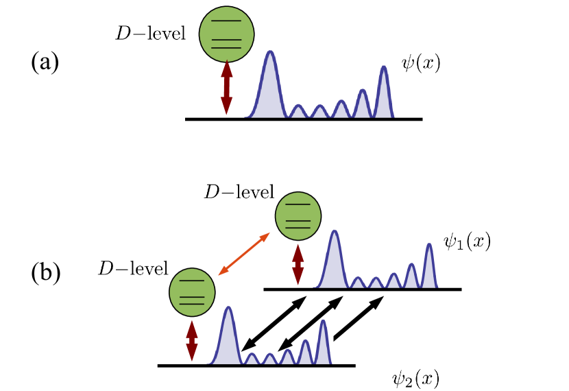
Figure 1: (color online) (a) The cMPS can be built by letting an ancilla (green circle in the figure) be coupled to a continuous field ($\psi(x)$). (b) In a similar way, we propose that coupled fields can also be constructed by coupling independent ancillas.

We review here the basics of continuous matrix product states (cMPS) for a single field. The cMPS are trial states for a variational estimation of ground states in one-dimensional quantum field theories. We start by considering a quantum system described in second quantization by means of the field operators $\hat{\psi}(z)$. According to the spin-statistics theorem, these operators must satisfy (anti)commutation relations $\hat{\psi}(z)\hat{\psi}^{\dagger}(z^{\prime})\pm\hat{\psi}^{\dagger}(z^{\prime})\hat{\psi}(z)=\delta(z-z^{\prime})$ according to whether they are fermions or bosons. Our system will be defined in a length $L$ with periodic boundary conditions.

The explicit form of the state can be written, as introduced in the seminal work of Verstraete and Cirac Cirac-Verstraete ($\hbar=1$ is used through the text)

$$|\chi\rangle={\rm tr_{aux}}\{\mathcal{P}{\rm e}^{\int_{0}^{L}{\rm d}z\,(Q(z)\otimes\mathbb{1}_{\mathcal{F}}+R(z)\otimes\hat{\psi}^{\dagger}(z))}\}|\Omega\rangle\;$$ (1)

where $\mathcal{P}$ denotes path-ordering (we follow the prescription in which, for the argument of the exponential, the value of $z$ increases as we move to the right). $Q(z)$ and $R(z)$ are complex $D\times D$ matrices acting on an auxiliary Hilbert space $\mathcal{H}_{\rm aux}$. The partial trace ${\rm tr_{aux}}$ is taken over $\mathcal{H}_{\rm aux}$. The suffix in $\mathbb{1}_{\mathcal{F}}$ emphasizes that it is the identity for the field. Finally, the state $|\Omega\rangle$ is the vacuum of a free theory,

$$\hat{\psi}(z)|\Omega\rangle=0$$ (2)

From now on, we will restrict ourselves to translational invariant setups in which the matrices $R$ and $Q$ become independent of $z$. The cMPS are complete Brockt2012 , i.e., any one dimensional quantum field can be casted in the form (1). This class of states can be obtained as the continuum limit of MPS, with bond dimension $D$. The bond dimension can be understood as a measure of the block entanglement. In one dimension the block entanglement saturates, thus, $D$ is expected to be sufficiently small. If so, we are able to reach any quantum state with a relatively small number of variational parameters ($2D^{2}$). This combined with the variational method results in a very powerful technique for finding ground-states of one-dimensional theories.

In a relativistic scenario, the block-entanglement has a UV logarithmic divergence. This can be understood since the ground state of a relativistic theory, also in $1+1$, will contain zero-point fluctuations from all energy scales, which are the ones contributing more to the entropy Srednicki1993 . A related argument due to Feynman is quoted in Ref. Haegeman2010, . The ground state will be dominated by the high energy contributions. As a consequence, in the variational procedure, the accuracy for describing the low-E sector is lost. Therefore, a cutoff must be introduced. Though challenging, the description of relativistic field theories has been succesfully described via cMPS introducing a regularization scheme Haegeman2010 ; Stojevic2014 . Here we will face the most favourable case of one dimensional non-relativistic theories.

Inherited from their discrete countenparts, the cMPS is not unique but the gauge transformation $Q\to gQg^{-1}$ and $R\to gRg^{-1}$ leaves the state $|\chi\rangle$ invariant Haegeman2013 . It turns out that the gauge

$$Q+Q^{\dagger}+R^{\dagger}R=0$$ (3)

is quite convenient. In this gauge, the cMPS state (1) can be rewritten as,

$$|\chi\rangle={\rm tr_{aux}}\{U(L,0)\}|\Omega\rangle$$ (4)

with

$$U(L,0)={\mathcal{P}}{\rm e}^{-i\int_{0}^{L}{\rm d}z(K\otimes\mathbb{1}_{\mathcal{F}}+iR\otimes\hat{\psi}^{\dagger}(z)-iR^{\dagger}\otimes\hat{\psi}(z))}$$ (5)

and, $K=K^{\dagger}$ Hermitean:

$$Q=-iK-\frac{1}{2}R^{\dagger}R\;,\;$$ (6)

which implies the gauge condition (3). The unitary operator $U$, in Eq. (5), is formally equivalent to a evolution in $z$-time for the field $\hat{\psi}(z)$ and a $D$-level (auxiliary) system with Hamiltonian $K$. Field and ancilla are coupled via $iR\otimes\hat{\psi}^{\dagger}(z)-iR^{\dagger}\otimes\hat{\psi}(z)$. The ground state is described in terms of the matrices $K$ and $R$, i.e., in terms of an auxiliary zero-dimensional system. This suggests an holographic interpretation for the cMPS Eisert . See Fig. 1(a) for a pictorial interpretation.

It remains to provide operational rules for computing within the cMPS formalism. To be precise, we must be able to write any field observable $\langle\chi|O(\hat{\psi},\hat{\psi}^{\dagger})|\chi\rangle$ in terms of the matrices $R$ and $Q$. As detailed in Ref. Rispler2012, , the following relations are found:

$$\langle\chi|\chi\rangle ={\rm tr}\{{\rm e}^{TL}\}$$ (7)

$$\langle\hat{\psi}^{\dagger}(z)\hat{\psi}(z)\rangle ={\rm tr}\{{\rm e}^{TL}(R\otimes R^{*})\}$$ (8)

$$\langle\partial_{z}\hat{\psi}^{\dagger}(z)\partial_{z}\hat{\psi}(z)\rangle ={\rm tr}\{{\rm e}^{TL}([Q,R]\otimes[Q^{*},R^{*}])\}$$ (9)

$$\langle\hat{\psi}^{\dagger}(z)\hat{\psi}^{\dagger}(z)\hat{\psi}(z)\hat{\psi}(z)\rangle ={\rm tr}\{{\rm e}^{TL}(RR\otimes R^{*}R^{*})\}$$ (10)

here,

$$T=Q\otimes\mathbb{1}+\mathbb{1}\otimes Q^{*}+R\otimes R^{*}$$ (11)

The Kronecker products in the ancilla space occurs because some identities, e.g., ${\rm tr}\{A\}{\rm tr}\{B\}={\rm tr}\{A\otimes B\}$, have been used.

To avoid those products in the auxiliary space, the isomorphism $|a\rangle|b\rangle\to|a\rangle\langle b^{*}|$ is introduced. This allows us to map vectors in $\mathcal{H}_{\rm aux}\otimes\mathcal{H}_{\rm aux}$ into operators acting on $\mathcal{H}_{\rm aux}$. This can be understood from the fundamental property

$${\rm tr}\Big{\{}\sum_{i}\sum_{abcd}A_{i}\otimes B_{i}^{*}|a\rangle|b\rangle\langle c|\langle d|\Big{\}}=$$

$${\rm tr}\Big{\{}\sum_{i}\sum_{abcd}|d^{*}\rangle\langle c|A_{i}|a\rangle\langle b^{*}|B_{i}^{\dagger}\Big{\}}\,.$$ (12)

The former also implies that operators acting on $\mathcal{H}_{\rm aux}$ are mapped into superoperators. Therefore, the action of $T$ on a ket $|\rho\rangle$ will be mapped into $\mathcal{T}[\rho]$, where $\mathcal{T}$ is a superoperator acting on the state (matrix) $\rho$. Under the isomorphism, it is straightforward to show that

$$\mathcal{T}[\varrho]:=-i[K,\varrho(z)]+R\varrho R^{\dagger}-\frac{1}{2}[R^{\dagger}R,\varrho(z)]_{+}$$ (13)

This is nothing but the dissipator governing a Linblad-like evolution ${\rm d}_{z}\varrho=\mathcal{T}\varrho$ for the irreversible dynamics of a system coupled to a reservoir. In this case, the role of the system is being played by the ancilla and that of the bath by the field (see Fig. 1(a) and the discussion above on the holographic interpretation). The Linbladian is a positive-semidefinite operator, $\mathcal{T}\leq 0$, having at least one zero eigenvalue Rivas2011 . With this at hand, Eq. (7) can be rewritten as

$$\langle\chi|\chi\rangle=\langle l|{\rm e}^{TL}r\rangle={\rm Tr}\Big{(}{\rm e}^{TL}|r\rangle\langle l|\Big{)}={\rm Tr}\Big{(}l\cdot{\rm e}^{\mathcal{T}L}r\Big{)}\;.$$

Here, $\langle l|$ and $|r\rangle$ are the left and right eigenvectors of $T$ (respectively) associated with its zero eigenvalue. We have assumed implicitly the limit $L\rightarrow\infty$ where this eigenvalue yields the principal contribution to the exponential. In the third equality, the above introduced isomorphism has been used. Note that the zero eigenvectors of $T$, under the isomorphism, are mapped into the stationary solutions of the Linblad equation (left and right equations). Accordingly, the action of $T$ into the bra $\langle l|$ can also be mapped into the action of a superoperator on a matrix: $\langle l|T\Leftrightarrow Q^{\dagger}l+\varrho_{l}Q+R^{\dagger}lR$. It is easy to see that, under the gauge (3), $l^{*}=\mathbb{1}$ is a solution of the stationary Linblad-like dynamics ($d_{z}l^{*}=0$). Combining all of this, we end up with

$$\langle\chi|\chi\rangle={\rm tr}(r^{*})=1$$ (14)

where $d_{z}r^{*}=0$.

In a similar way, we can re-express the expectation value of any operator in terms of the steady-state solution $\varrho^{*}$ of the right Linblad equation

$$\langle\hat{\psi}^{\dagger}(z)\hat{\psi}(z)\rangle= {\rm tr}\left(R^{\dagger}R\varrho^{*}\right)$$ (15)

$$\langle\partial_{z}\hat{\psi}^{\dagger}(z)\partial_{z}\hat{\psi}(z)\rangle= {\rm tr}\left([Q,R]^{\dagger}[Q,R]\varrho^{*}\right)$$ (16)

$$\langle\hat{\psi}^{\dagger}(z)\hat{\psi}^{\dagger}(z)\hat{\psi}(z)\hat{\psi}(z)\rangle= {\rm tr}\left((R^{\dagger})^{2}R^{2}\varrho^{*}\right)$$ (17)

With this we conclude our overview of the cMPS formalism. In the limit $L\rightarrow\infty$, we will be concerned with the ground state energy density $e_{0}=\langle\chi|\hat{{\mathcal{H}}}(\psi,\psi^{\dagger})|\chi\rangle$ (where $\hat{{\mathcal{H}}}$ is the Hamiltonian density operator). The latter can be computed by minimizing with the matrices $R$ and $Q$ as input and using the latter relations (and similar ones). Once the minimization procedure has finished, observables can be computed with the same relations using the optimized matrices.

III Application to Luttinger liquids

III.1 Bosonization

At low temperatures, a large class of one dimensional theories exhibit excitations of bosonic nature and their correlation functions are characterized by power laws. An interesting feature of 1D is that this class makes almost no distinction between bosons and fermions. HaldaneHaldane1 ; Haldane2 termed this class of theories Luttinger liquids. The bosonic nature of the low-energy excitations in 1D is due to the enhanced role quantum fluctuations acquire in low dimensional systems.

For a given microscopic model, the so-called bosonization prescription, consists in expressing the original degrees of freedom in terms of new fields which capture the collective behaviour characterizing the low-energy regime. For the case of a bosonic field, we will introduce the density-phase representationgiamarchi

$$\hat{\psi}^{\dagger}(x)=\sqrt{\hat{\rho}(x)}{\rm e}^{-i\hat{\theta}(x)}$$ (18)

where $\hat{\rho}(x):=\psi^{\dagger}(x)\psi(x)$ is the particle density field and $\hat{\theta}(x)$ the phase field. Close enough to the ground state we can safely approximate the density operator by

$$\hat{\rho}(x)\sim\rho_{0}-\frac{1}{\pi}\partial_{x}\hat{\phi}(x)$$ (19)

where $\rho_{0}$ is the ground state density and the operator $\hat{\phi}(x)$ characterizes the fluctuations over the ground state. The commutation relations for bosonic fields will translate into a canonical commutation relation for the $\hat{\theta}$ and $\hat{\phi}$ fields

$$[\frac{1}{\pi}\partial_{x}\hat{\phi}(x),\hat{\theta}(x^{\prime})]=-i\delta(x-x^{\prime})$$ (20)

III.2 Calculation for the Lieb-Liniger model

We are going to apply the previous ideas to the Lieb-Liniger model Lieb-Liniger1 . The former describes a $1$D non-relativistic bosonic gas interacting via a repulsive zero-range potential

$$\hat{H}=\int_{0}^{L}{\rm d}x\,\frac{1}{2M}\partial_{x}\hat{\psi}^{\dagger}(x)\partial_{x}\hat{\psi}(x)+c\,(\hat{\psi}^{\dagger}(x))^{2}(\hat{\psi}(x))^{2}$$ (21)

The Lieb-Liniger model is exactly solvable by means of a Bethe ansatz. In fact, the solution shows that at low-energies, this model displays a Luttinger liquid behaviour Lieb-Liniger2 . An excellent agreement between the exact ground state energy density and the cMPS solution has already been provided Cirac-Verstraete . Finally, note that this model conserves the particle number density. This quantity will represent a minimization constraint when finding the ground state numerically.

Following the bosonization scheme, the effective Hamiltonian describing the low-energy behaviour of the Lieb-Liniger model is

$$\hat{H}_{\rm eff}=\frac{v}{2\pi}\int_{0}^{L}{\rm d}x\,K(\partial_{x}\hat{\phi}(x))^{2}+\frac{1}{K}(\partial_{x}\hat{\theta}(x))^{2}$$ (22)

Hence, the low-energy regime can be completely characterized by means of two parameters (Luttinger parameters): the velocity $v$ and the dimensionless parameter $K$. These, in turn, can be related to the ground state energy density $e_{0}(\rho)$ of the microscopic Hamiltonian (21). The corresponding relations are Cazalilla1

$$v^{2}=\frac{\rho_{0}}{M}\left.\frac{\partial^{2}e_{0}}{\partial\rho^{2}}\right|_{\rho=\rho_{0}}$$ (23)

$$K^{2}=\frac{\pi^{2}\rho_{0}}{M}\left(\left.\frac{\partial^{2}e_{0}}{\partial\rho^{2}}\right|_{\rho=\rho_{0}}\right)^{-1}\;.$$ (24)

It is possible to obtain asymptotic (analytic) expressions for the former parameters in terms of the dimensionless coupling constant $\gamma=Mc/\rho_{0}$. In Fig. 2 we compare those asymptotic limits (small and large repulsion, see Ref. Cazalilla1, ) for $v$ and $K$ with (23) and (24) as obtained from the ground state energy density computed with cMPS. We have performed simulations for $D=2$, $4$, $6$ and $8$. For every bond dimension, the ground state energy density was calculated for up to twelve different densities. By interpolation, we constructed the continuous function $e_{0}(\rho)$ and the derivatives were calculated from it. Results show that for a moderately small bond dimension ($D=6$), it is possible to match the predicted asymptotic behaviour up to high values of $\gamma$. Results for $D=2$ are not shown for the sake of clarity (such a small bond dimension does not capture correctly the ground state of the Lieb-Liniger model).

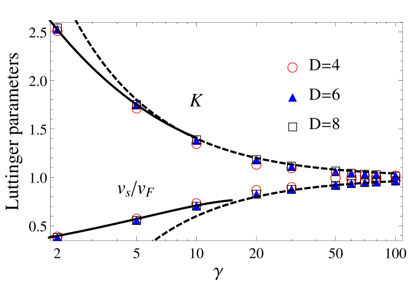
Figure 2: (color online) Luttinger parameters as a function of the dimensionless zero-range interaction constant $\gamma=Mc/\rho_{0}$ (we choose $\rho_{0}=1$ and $M=1/2$). The full and dashed lines correspond to the weak and strong repulsion limits (respectively). These are compared with our cMPS results for bond dimensions $D=4$ (open circles), $6$ (filled triangles) and $8$ (open squares).

IV Extension/Generalization for coupled fields

The cMPS formalism can be naturally extended to treat a multi-species system. Let us consider a system of length $L$ in which coexist $q$ bosonic and/or fermionic particle species which are annihilated by the operators $\hat{\psi}_{\alpha},\,\,\alpha=1,...,q$. These operators satisfy (anti)commutation relations

$$\hat{\psi}_{\alpha}(x)\hat{\psi}_{\beta}(x^{\prime})-\eta_{\alpha\beta}\hat{\psi}_{\beta}(x^{\prime})\hat{\psi}_{\alpha}(x) = 0$$ (25)

$$\hat{\psi}_{\alpha}(x)\hat{\psi}^{\dagger}_{\beta}(x^{\prime})-\eta_{\alpha\beta}\hat{\psi}_{\beta}^{\dagger}(x^{\prime})\hat{\psi}_{\alpha}(x) = \delta_{\alpha\beta}\delta(x-x^{\prime})$$ (26)

where $\eta_{\alpha\beta}=+1$ if at least one of the fields $\alpha$ or $\beta$ is bosonic and $\eta_{\alpha\beta}=-1$ if both fields are of fermionic nature.

The $q$-species cMPS state is defined as (Haegeman, )

$$|\chi\rangle={\rm tr_{aux}}\{B\mathcal{P}{\rm e}^{\int_{0}^{L}{\rm d}z\,\tilde{Q}(z)\otimes\mathbb{1}+\sum_{\alpha=1}^{q}\tilde{R}_{\alpha}(z)\otimes\hat{\psi}_{\alpha}^{\dagger}(z)}\}|\Omega\rangle\;,$$ (27)

here, matrices $\tilde{R}_{\alpha}$ have been introduced for each one of the fields $\hat{\psi}_{\alpha}$ and a single Hamiltonian $\tilde{K}$ for the auxiliary system. We will employ the tilde notation for the variational parameters of the multi-species cMPS state to differentiate them from their single field counterparts, cf. Eq. (1). The matrix $\tilde{Q}$ is now defined as

$$\tilde{Q}(x)=-i\tilde{K}(x)-\frac{1}{2}\sum_{\alpha=1}^{q}\tilde{R}_{\alpha}^{\dagger}(x)\tilde{R}_{\alpha}(x)$$ (28)

At difference with the single field case, a regularity condition must be imposed on the $\tilde{R}_{\alpha}$ matrices in order that the expectation value of the non-relativistic kinetic energy, as computed with (27), will not become divergent. This condition reads

$$\tilde{R}_{\alpha}(x)\tilde{R}_{\beta}(x)-\eta_{\alpha\beta}\tilde{R}_{\beta}(x)\tilde{R}_{\alpha}(x)=0$$ (29)

In other words, the matrices $\tilde{R}_{\alpha}$ inherit the (anti)commutation relation of their corresponding fields. With these ideas in mind we can extend the operational rules for computing expectation values with cMPS. For example,

$$\langle\chi|\chi\rangle={\rm tr}\{{\rm e}^{\tilde{T}L}\}\;,$$ (30)

where the transfer operator (11) has been generalized to

$$\tilde{T}=\tilde{Q}\otimes\mathbb{1}+\mathbb{1}\otimes\tilde{Q}^{*}+\sum_{\alpha=1}^{q}\tilde{R}_{\alpha}\otimes\tilde{R}_{\alpha}^{*}$$ (31)

and translational invariance has been assumed for simplicity.

Special care must be taken into account for systems where two or more fermionic species coexist. Let us discuss correlators like $\langle\hat{\psi}_{\alpha}^{\dagger}(x)\hat{\psi}_{\beta}(y)\rangle$. Expanding the path-ordered exponential in (27), which acts on the vacuum $|\Omega\rangle$ of the field theory, and taking the annihilation operators to the right (normal ordering prescription) we obtain Haegeman

$$\langle\hat{\psi}_{\alpha}^{\dagger}(x)\hat{\psi}_{\beta}(y)\rangle={\rm tr}\{ {\rm e}^{\tilde{T}y}(\tilde{R}_{\beta}\otimes\mathbb{1}){\rm e}^{\tilde{T}_{\alpha}(x-y)}$$

$$\times(\mathbb{1}\otimes\tilde{R}_{\alpha}^{*}){\rm e}^{\tilde{T}(L-x)}\}$$ (32)

($x>y$) where the generalized transfer operator $\tilde{T}_{\alpha}$ deals with the exchange statistics

$$\tilde{T}_{\alpha} = \tilde{Q}\otimes\mathbb{1}+\mathbb{1}\otimes\tilde{Q}^{*}+\sum_{\beta=1}^{q}\eta_{\alpha\beta}\tilde{R}_{\beta}\otimes\tilde{R}_{\beta}^{*}$$ (33)

For the case of bosonic systems, $\tilde{T}_{\alpha}=\tilde{T}$. The transfer operator $\tilde{T}$ governs the evolution of states in the ancillary space. Similarly to the single field case, this evolution can be mapped to a dissipative dynamics corresponding to the following Linblad quantum master equation

$$\frac{d\tilde{\varrho}(z)}{dz}=-i[\tilde{K},\tilde{\varrho}(z)]+\sum_{\alpha=1}^{q}\tilde{R}_{\alpha}\tilde{\varrho}\tilde{R}_{\alpha}^{\dagger}-\frac{1}{2}[\tilde{R}_{\alpha}^{\dagger}\tilde{R}_{\alpha},\tilde{\varrho}(z)]_{+}$$ (34)

Thus, we have again the picture of the ancilla coupled to a bath (the fields) by means of the operators $\tilde{R}_{\alpha}$.

Consider now the case of two bosonic fields $\hat{\psi}_{1}$ and $\hat{\psi}_{2}$. We are interested in studying how the matrices ($\tilde{R}_{\alpha}$ and $\tilde{K}$), which define the cMPS state in this two-species system, can be constructed from the matrices which characterize a single field. The simplest scenario considers two uncoupled fields. We have seen how the problem of computing expectation values in the ground state can be reduced to a dissipative dynamics going on in the auxiliary space - where the state of the total auxiliary system is described in terms of the density matrix $\tilde{\rho}$. In the absence of a coupling between the fields, we should be able to recover our single field solutions. This is nothing but to demand the density matrix to be separable, that is, $\tilde{\varrho}=\varrho_{1}\otimes\varrho_{2}$. Both fields do not need to be identical, therefore, each of them will have associated a different set of matrices $R_{\alpha}$ and $K_{\alpha}$ which act on the corresponding auxiliary space $\mathcal{A}_{\alpha}$. For simplicity, we assume that both $\mathcal{A}_{1}$ and $\mathcal{A}_{2}$ have the same bond dimension $D_{1}=D_{2}=D$. The total auxiliary space for the two fields will be the tensor product of the individual spaces $\tilde{\mathcal{A}}=\mathcal{A}_{1}\otimes\mathcal{A}_{2}$. Due to the tensor product structure, the bond dimension of the total auxiliary space is now $\tilde{D}=D^{2}$. The ancillas evolve independently according to the total Hamiltonian

$$\tilde{K}=K_{1}\otimes\mathbb{1}+\mathbb{1}\otimes K_{2}$$ (35)

Similarly, each auxiliary system will couple to its quantum field by means of the matrices $R_{\alpha}$. The extension of these to the product space is

$$\tilde{R}_{1}=R_{1}\otimes\mathbb{1}$$ (36)

$$\tilde{R}_{2}=\mathbb{1}\otimes R_{2}$$ (37)

Notice that the matrices $\tilde{R}_{\alpha}$ satisfy the bosonic commutation relation $[\tilde{R}_{1},\tilde{R}_{2}]=0$ as it is demanded for a multi-species system (29). As desired, our construction let us recover the results for single fields. For instance, $\langle\hat{\psi}_{1}^{\dagger}\hat{\psi}_{1}\rangle={\rm tr}(\tilde{\rho}^{*}\tilde{R}_{1}^{\dagger}\tilde{R}_{1})={\rm tr}(\rho_{1}^{*}R_{1}^{\dagger}R_{1}){\rm tr}\rho_{2}^{*}={\rm tr}(\rho_{1}^{*}R_{1}^{\dagger}R_{1})$ (as ${\rm tr}\rho_{2}^{*}=1$ for a density matrix).

How is this picture modified in the presence of a coupling between $\hat{\psi}_{1}$ and $\hat{\psi}_{2}$? An arbitrary operator $\tilde{C}$, mapping $\tilde{\mathcal{A}}$ into itself, can be represented as $\tilde{C}=\sum_{i}c_{i}A_{i}\otimes B_{i}$, where $A_{i}$ acts on $\mathcal{A}_{1}$ and $B_{i}$ acts on $\mathcal{A}_{2}$. Therefore, this defines the most general structure for the matrices $\tilde{R}_{\alpha}$ and $\tilde{K}$. Those general matrices must satisfy the regularity conditions (29), which complicates their construction.

A possible solution is the following. We use the intuitive interpretation for the cMPS in terms of a system-bath, see Fig. 1(b) and the discussion on the holographic interpretation below Eq. (13). Starting from the decoupled solution (35), (36) and (37), we switch on the coupling adiabatically and expect that our solutions will start to modify. This is depicted schematically in Fig. 1(b). Here, as one introduces the coupling between the physical fields, the individual auxiliary spaces will also start to interact. Inspired by this procedure, we propose the following construction in the presence of a coupling. First of all, the matrices $\tilde{R}_{1}$ and $\tilde{R}_{2}$ will continue to be described by (36) and (37) respectively. In this way, we guarantee that they commute, satisfying (29) trivially. In order to render the state non-separable, the matrix $\tilde{K}$ is written in a general way but containing the uncoupled solution as a limit (35). This is done as follows

$$\tilde{K}=K_{1}\otimes\mathbb{1}+\mathbb{1}\otimes K_{2}+\sum_{p=0}^{P}Z_{1}^{(p)}\otimes Z_{2}^{(p)}$$ (38)

where $Z_{1}^{(0)}=Z_{2}^{(0)}=0$. In order to keep $\tilde{K}$ Hermitean, we will demand that the matrices $Z_{i}^{(p)}$ are Hermitean too. The number $P$ of pairs of $Z$ matrices is arbitrary. In principle, we will expect it to grow with the strength of the coupling.

We have seen for the single field case, that the cMPS ansatz is able to map the properties of a continuous one-dimensional field theory by means of $2D^{2}$ variational parameters (with of course, a relatively small bond dimension $D$). Doubling the number of fields, as well as introducing $P$ pairs of the already defined $Z$ matrices, increases the total number of variational parameters to $(4+2P)D^{2}$.

V Two-species bosonic system

The system we have in mind to test the cMPS method for coupled fields is a two-component bosonic system. Binary systems of this kind (as well as bosonic + fermionic mixtures) are Luttinger liquids with a rich phase diagram Cazalilla2 ; Mathey . We will consider two Lieb-Liniger gases with a density density coupling. This is described by the following Hamiltonian:

$$\hat{H}=\frac{1}{2M}\sum_{\alpha=1}^{2} \int_{0}^{L}{\rm d}x\,\partial_{x}\hat{\psi}_{\alpha}^{\dagger}(x)\partial_{x}\hat{\psi}_{\alpha}(x)$$

$$+c\sum_{\alpha=1}^{2} \int_{0}^{L}{\rm d}x\,\big{(}\hat{\psi}_{\alpha}^{\dagger}(x)\big{)}^{2}\big{(}\hat{\psi}_{\alpha}(x)\big{)}^{2}$$

$$+g \int_{0}^{L}{\rm d}x\,\hat{\rho}_{1}(x)\hat{\rho}_{2}(x)$$ (39)

In order to obtain the low-energy behaviour of this model we will use the bosonization technique introduced in Sect. III.1. As already explained, this consists in rewriting the bosonic fields in terms of the collective fields $\hat{\theta}_{\alpha}$ and $\hat{\phi}_{\alpha}$ which characterize the bosonic low-energy excitations. Hamiltonian (V) conserves the individual particle densities, $[\hat{H},\hat{\rho}_{\alpha}]=[\hat{H},\hat{\rho}]=0$ ($\alpha=1,2$). Therefore, we can fix these two densities as minimization constraints in the cMPS procedure. In Eq. (19), we have considered the lowest order term in a harmonic expansion of the density operator. A more careful treatmentgiamarchi shows that, the correct expansion for the density operator in terms of the field $\hat{\phi}_{\alpha}$ is of the form $\hat{\rho}_{\alpha}(x)=[\rho_{0\alpha}-\partial_{x}\hat{\phi}_{\alpha}(x)/\pi]\sum_{p}{\rm e}^{i2p(\pi\rho_{0\alpha}x-\hat{\phi}_{\alpha}(x))}$. Our former simplification is justified due to the fact that, at long distances (low-energies), the phase terms oscillate very fast and will average to zero upon integration. In performing the bosonization, we must retain the most dominant terms at low-energies. For the case of our inter-species coupling, this supposes to consider also the first harmonic $p=1$. This leads, at low temperatures, to a coupling contribution of the form: $1/2\pi\int{\rm d}x\,[2g_{x}\partial_{x}\hat{\phi}_{1}\partial\hat{\phi}_{2}+g_{c}\cos(2(\hat{\phi}_{1}-\hat{\phi}_{2})+\pi\delta x)]$ (with $\delta=\rho_{01}-\rho_{02}$). Of particular interest for us will be the case of equal filling $\rho_{01}=\rho_{02}$ ($\delta=0$). Species $1$ and $2$ in the low-energy effective Hamiltonian can be decoupled by introducing the normal modes $\hat{\phi}_{+}=1/\sqrt{2}(\hat{\phi}_{1}+\hat{\phi}_{2})$ and $\hat{\phi}_{-}=1/\sqrt{2}(\hat{\phi}_{1}-\hat{\phi}_{2})$. In terms of these we have that the low-energy excitations of (V) can be described by the effective Hamiltonian

$$\hat{H}_{\rm eff}=\frac{1}{2\pi}\int{\rm d}x\,\Big{[} \sum_{\nu=\pm}v_{\nu}\left((\partial_{x}\hat{\phi}_{\nu})^{2}+\frac{1}{K_{\nu}}(\partial_{x}\hat{\theta}_{\nu})^{2}\right)$$

$$+g_{c}\cos(\sqrt{8}\hat{\phi}_{-})\Big{]}$$ (40)

Similarly to the single field case, the Luttinger parameters $v_{\pm}$ and $K_{\pm}$ can be related to the ground state energy density $e_{0}(\rho_{+},\rho_{-})$ (as a function of the normal densities) of Hamiltonian (V).

$$v_{\pm}^{2} =\frac{2\rho_{0\pm}}{M}\left.\frac{\partial^{2}e_{0}}{\partial\rho_{\pm}^{2}}\right|_{\rho_{\pm}=\rho_{0\pm}}$$ (41)

$$K_{\pm}^{2} =\frac{\pi^{2}\rho_{0\pm}}{2M}\left(\left.\frac{\partial^{2}e_{0}}{\partial\rho_{\pm}^{2}}\right|_{\rho_{\pm}=\rho_{0\pm}}\right)^{-1}$$ (42)

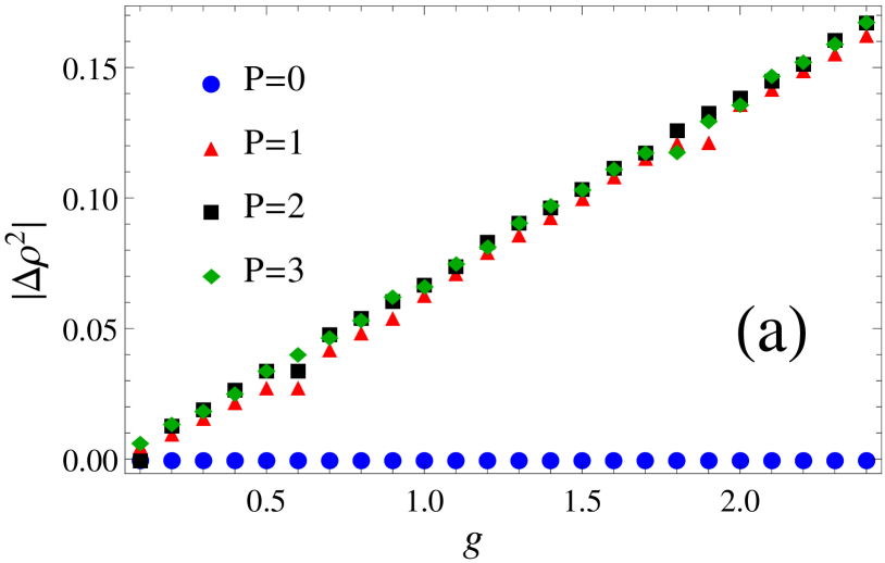
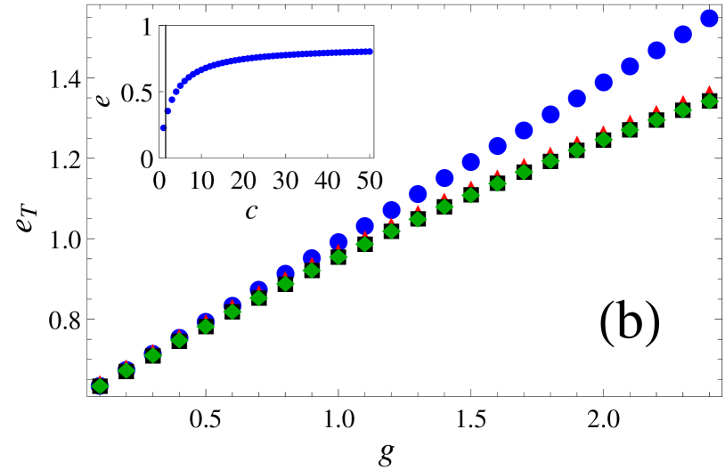
Figure 3: (color online) (a) Ground state density-density correlations and (b) total energy density for Hamiltonian (V). Both as a function of the interspecies coupling strength $g$ for equal densities $\rho_{01}=\rho_{02}=0.63$ and $c=1.5$. The ancilla space for each field has bond dimension $D$ equal to $6$. We couple the ancillas by means of $P$ pairs of $Z$ matrices. Results are shown for $P=0$ (circles), $P=1$ (triangles), $P=2$ (squares) and $P=3$ (diamonds). Inset: ground state energy density for a single Lieb-Liniger chain as a function of $c$ ($D=6$). The vertical line denotes the value of $c$ at which we are coupling two fields.

Coupled species have been thoroughly studied Cazalilla2 ; Mathey . In this work we study coupled bosonic species described by (V). The range of parameters considered coincides with the one in Refs. Kleine, ; Kleine-thesis, where a DMRG study is reported, hence a direct comparison is possible.

In Fig. 3 (a) we plot the ground state density-density correlations $|\Delta\rho^{2}|=|\langle\hat{\rho}_{1}(x)\hat{\rho}_{2}(x)\rangle-\langle\hat{\rho}_{1}(x)\rangle\langle\hat{\rho}_{2}(x)\rangle|$ as a function of the interspecies coupling $g$ for different values of $P$. Both, the repulsion strength $c$ and the bond dimension $D$ are kept fixed ($c=1.5$ and $D=6$). As expected, $P=0$ renders the state separable and no correlations are observed. Making $P\neq 0$ the correlations between the two fields build up. They grow with the coupling strength. In this range of parameters, $P=2$ seems to be sufficient for account with the physics.

The ground state energy density as a function of $g$ is shown in Fig. 3 (b). Only the last term of (V) depends on $g$, therefore, (for a fixed value of $c$) the first two terms yield a constant contribution. The case $P=0$ yields a mean field treatment where the interaction is replaced by $g\langle\hat{\rho 1}\rangle\langle\hat{\rho_{2}}\rangle$. It was already mentioned that $[\hat{H},\hat{\rho}_{1}]=[\hat{H},\hat{\rho}_{2}]=0$. Thus, with $P=0$, the energy as a function of $g$ has a linear dependence with slope $\rho_{01}\rho_{02}$. Including quantum correlations ($P\neq 0$) the energy is no longer a linear function of the coupling, as seen in 3 (b).

As it was already discussed, the low-energy description of our model is characterized by the Luttinger parameters (41) and (42). In particular, the difference in normal velocities $v_{\pm}$ yields the charge-spin separation - a typical experimental characteristic in mixtures. In Fig. 4 we compare for both the $v_{\pm}$ and $K_{\pm}$ our cMPS results with the DMRG values extracted from Refs. Kleine, ; Kleine-thesis, . Let us remark the excellent agreement in $K_{+}$ and $v_{+}$ and the minor discrepancy in $K_{-}$ or $v_{-}$. The very small differences could be attributed to a number of issues: small bond dimension in the cMPS ($D=6$) to be compared with the DMRG (several hundreds), or the fact that the DMRG theory is discretized an the cMPS is fully continuous.

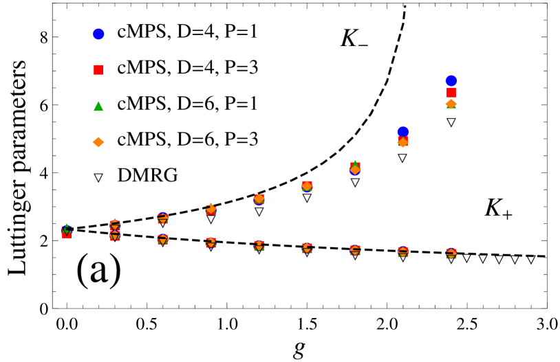
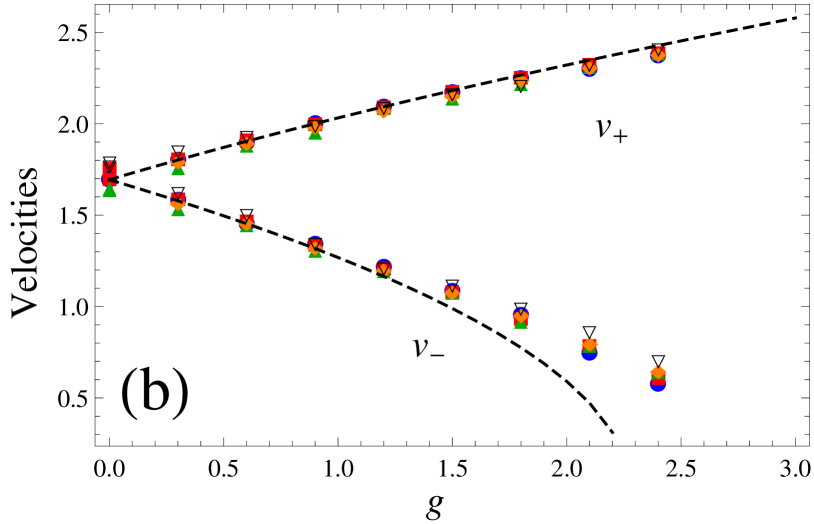
Figure 4: (color online) Charge(+) and spin(-) Luttinger parameters as a function of the coupling $g$ between fields. Here we show a comparison between a weak-coupling approximation (dashed line), DMRG Kleine and our results implementing cMPS for coupled fields with different bond dimensions and values of the parameter $P$ for fixed $c=1.5$. (a) $K_{\pm}$ (b) velocities $v_{\pm}$.

VI Quantum simulation of coupled cMPS

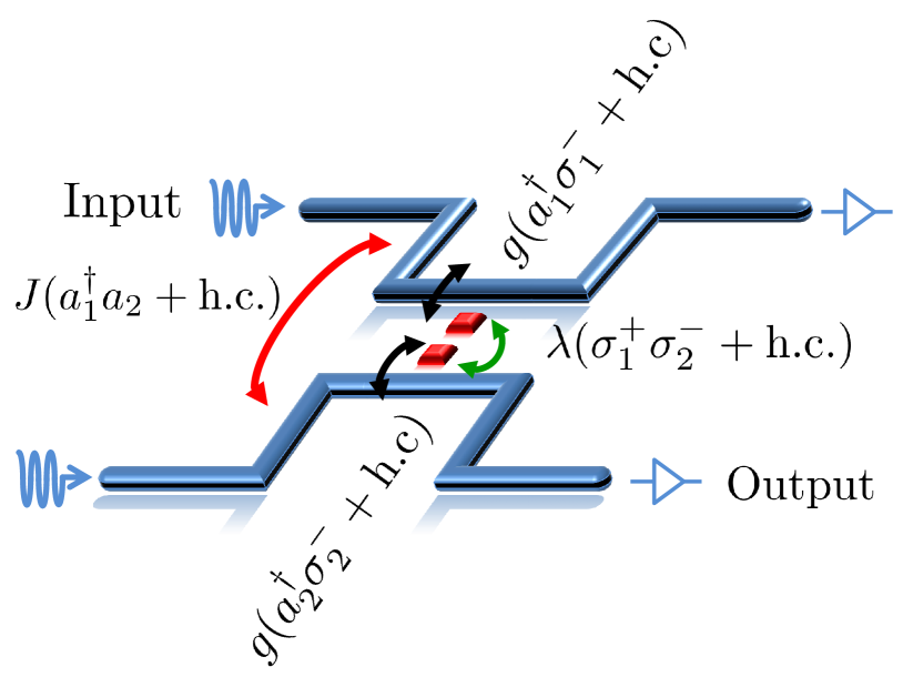
Figure 5: (color online) Possible circuit QED implementation for the quantum simulation of a cMPS for two coupled fields. The ancillas consist on two cavity-qubit setups and the fields are the input and output of the EM field. The Hamiltonian of the cavity-qubit setups simulates $\tilde{K}$ and the cavity operators couple to the external field, that is, they correspond to the matrices $\tilde{R}_{\alpha}$.

There exist two approaches towards the quantum simulation of continuous or discrete field theories Nori . The conventional one consists on taking a flexible quantum system, such as a Bose-Einstein condensate, ultracold atoms in an optical lattice or a superconductor, and working with it to implement the full field theory, or an approximate version of it, in the experiment. This “analogue” quantum simulator therefore evolves and equilibrates as the original model dictates and all observables may be directly studied on the experiment itself.

A second possibility for quantum simulation arises from the physical interpretation of cMPS. The idea is that there exists a mapping between a continuous Matrix Product state and a physical process operating on a small quantum mechanical object. This mapping between states and channels was already evidenced for discrete MPSSchon2005 ; Schon2007 and has been recently generalized for cMPSBarrett2013 , by means of their physical interpretation in terms of a system (the ancilla) coupled to a bath (the field). The beauty of this mapping is that it is quite general and applies to a variety of quantum optical systems. The prototypical system is an atom-cavity setup (the system or ancilla in the language of this paper) that interacts with external input and output fields through the bath (the field in cMPS) in this case the electromagnetic field. However, any other quantum discrete system coupled to an outer field, where different order correlations of the latter can be measured, such as circuit QED Wallraff2004 ; You2011 would do the job.

Let us now summarize the proposal in Ref. Barrett2013, . The atom-cavity system is described through the well known Jaynes-Cummings (JC) model,

$$\hat{H}_{\rm ancilla}=\hat{H}_{\rm JC}=\Omega\hat{a}^{\dagger}\hat{a}+\epsilon\hat{\sigma}^{+}\hat{\sigma}^{-}+g(\hat{a}^{\dagger}\hat{\sigma}^{-}+{\rm h.c})$$ (43)

here $\hat{a}$ ($\hat{a}^{\dagger}$) are bosonic annihilation (creation) operators describing the main stationary mode of a cavity. The atom (with two relevant states splitted by $\epsilon$) is coupled to this fundamental mode of $\Omega$-frequency with a strength $g$. The $\hat{\sigma}^{-}$ ($\hat{\sigma}^{+}$) are lowering (raising) operators for the two-level system. The atom-cavity is coupled to an EM-environment, that in second quantization is given by the free Hamiltonian, $\hat{H}_{\rm EM}=\int{\rm d}\omega\,\omega\,\hat{b}^{\dagger}(\omega)\hat{b}(\omega)$. Taking an interaction picture with respect to the EM field, the system-bath (ancilla-field) coupling can be written as

$$\hat{H}_{\rm coupling}(t)=\sqrt{\frac{\kappa}{2\pi}}\int{\rm d}\omega\,\hat{a}^{\dagger}\hat{b}(\omega){\rm e}^{-i\omega t}+{\rm h.c.}$$ (44)

Limiting the integration region to frequencies $\omega$ near $\Omega$ we can safely assume the RWA. Also, assuming a point-like interaction in space, the coupling function is flat in momentum. It is customary to introduce the time dependent operators $\hat{E}^{+}(t)=i/\sqrt{2\pi}\int{\rm d}\omega\,{\rm e}^{-i\omega t}\hat{b}(\omega)$ and Hermitian conjugate. They correspond to the electric field components of the EM field. In this way, we can finally write the total Hamiltonian as

$$\hat{H}(t)=\hat{H}_{\rm ancilla}+i\sqrt{\kappa}(\hat{a}\otimes\hat{E}^{-}(t)-{\rm h.c.})$$ (45)

The electric field operators can, in turn, be decomposed into in-out componentsGardiner1985 . The in component corresponds to the field that impinges on the system while the out component consists of a reflected part plus a radiated one due to the interaction of the EM field with the system. If we take the in state of the EM field to be the vacuum, it can be shownGardiner-Zoller that the evolution governed by (45) can be reduced to that of the non-Hermitian Hamiltonian

$$-i\hat{H}_{\rm eff}(t)=-i\hat{H}_{\rm ancilla}-\frac{1}{2}\kappa\hat{a}^{\dagger}\hat{a}+\sqrt{\kappa}\hat{a}\otimes\hat{E}^{-}(t)$$ (46)

This is the same kind of evolution which generates the cMPS ansatz (see Eqs. (1) and (6)) once we trace over the degrees of freedom of the ancilla. We thus make the following identification:

$$R=\sqrt{\kappa}\hat{a}\qquad K=\hat{H}_{\rm ancilla}(\Omega,\epsilon,g)$$ (47)

While we do not have control over $R$, we can modify the variational parameter $K$ by properly tuning the couplings ($\Omega$,$\epsilon$,$g$) of the cavity-atom system. The continuous field $\hat{\psi}(x)$ will map into the output field operators of the electromagnetic field: $\hat{\psi}(x)=\hat{E}^{+}(t)$. Being the EM field in a cMPS state, computing expectation values of operators will translate into measuring correlations of the EM field itself, i.e., measuring the normalized correlation functions $g^{(1)}(t,t^{\prime})$, $g^{(2)}(t,t^{\prime})$

$$g^{(1)}(t,t^{\prime}) = \frac{\langle\hat{E}^{-}(t)\hat{E}^{+}(t^{\prime})\rangle}{\sqrt{\langle\hat{E}^{-}(t)\hat{E}^{+}(t)\rangle\langle\hat{E}^{-}(t^{\prime})\hat{E}^{+}(t^{\prime})\rangle}}$$ (48)

$$g^{(2)}(t,t^{\prime}) = \frac{\langle\hat{E}^{-}(t)\hat{E}^{-}(t^{\prime})\hat{E}^{+}(t)\hat{E}^{+}(t^{\prime})\rangle}{\langle\hat{E}^{-}(t)\hat{E}^{+}(t)\rangle\langle\hat{E}^{-}(t^{\prime})\hat{E}^{+}(t^{\prime})\rangle}$$ (49)

and higher orders depending on the model we wish to simulate. Following our previous identification, the correlators $\langle\hat{E}^{-}(t)\hat{E}^{+}(t^{\prime})\rangle$ and $\langle\hat{E}^{-}(t)\hat{E}^{-}(t^{\prime})\hat{E}^{+}(t)\hat{E}^{+}(t^{\prime})\rangle$ map to $\langle\hat{\psi}^{\dagger}(x)\hat{\psi}(x^{\prime})\rangle$ and $\langle\hat{\psi}^{\dagger}(x)\hat{\psi}^{\dagger}(x^{\prime})\hat{\psi}(x)\hat{\psi}(x^{\prime})\rangle$ respectively. It was shown numerically that the atom-cavity setup could simulate the Lieb-Liniger model giving correlations acceptably well Barrett2013 .

With this work at hand, our proposal has also a natural realization. In our case, we envision two superconducting cavities interacting each one with oneSun2014 ; Mariantoni2008 ; Reuther2010 or several superconducting qubits (Fig. 5):

$$\hat{H}_{\rm sys}=\sum_{\alpha}g\hat{a}_{\alpha}^{\dagger}\hat{\sigma}_{\alpha}^{-}+J\hat{a}_{\alpha}^{\dagger}\hat{a}_{\alpha+1}+\lambda\hat{\sigma}_{\alpha}^{+}\hat{\sigma}^{-}_{\alpha+1}+{\rm h.c.}$$ (50)

That are coupled to different baths (different fields) through

$$\hat{H}_{\rm coupling}(t)=\sum_{\alpha}\sqrt{\kappa_{\alpha}}\int{\rm d}\omega\,\hat{a}_{\alpha}^{\dagger}\hat{b}_{\alpha}(\omega){\rm e}^{-i\omega t}+{\rm h.c.}$$ (51)

Therefore in our case ($\alpha=1,2$), the identifications are the following,

$$\tilde{R}_{\alpha}=\sqrt{\kappa_{\alpha}}\hat{a}_{\alpha}$$ (52)

and

$$\widetilde{K}=\hat{H}_{\rm sys}$$ (53)

with

$$K_{\alpha}=\hat{H}_{\rm JC,\alpha}=g\hat{a}_{\alpha}^{\dagger}\hat{\sigma}_{\alpha}^{-}+{\rm h.c.}$$ (54)

and

$$Z_{1}^{(1)}\otimes Z_{2}^{(1)}+Z_{1}^{(2)}\otimes Z_{2}^{(2)}=J\hat{a}_{1}\otimes\hat{a}^{\dagger}_{2}+{\rm h.c.}$$ (55)

and

$$Z_{1}^{(3)}\otimes Z_{2}^{(3)}+Z_{1}^{(4)}\otimes Z_{2}^{(4)}=\lambda\hat{\sigma}_{1}^{+}\otimes\hat{\sigma}_{2}^{-}+{\rm h.c.}$$ (56)

Note that in Sect.IV we demanded that the matrices $Z$ should be Hermitian. Eqs. (55) and (56) can always be brought into a sum of tensor products of Hermitian operators. The former equations are of the form $C=A\otimes B^{\dagger}+A^{\dagger}\otimes B$. We can split any operator in terms of its Hermitian components. In the case of $A$, the decomposition reads: $A=A_{r}+iA_{i}$ (and similarly for $B$). Here, $A_{r}=1/2(A^{\dagger}+A)$ and $A_{i}=i/2(A^{\dagger}-A)$. It is straightforward to show that $C$ can be rewritten as: $C=2A_{r}\otimes B_{r}+2A_{i}\otimes B_{i}$.

Finally, as for the single field, EM field correlations need to be computed. In addition, cross-correlations, for instance, $\langle\hat{E}_{i}^{-}(t)\hat{E}_{j}^{+}(t^{\prime})\rangle$ will be necessary. In circuit QED this is possible as reported in the literature Eichler2011 ; DiCandia2014 ; Menzel2010 ; Bozyigit2010 ; Bozyigit2011 .

VII Summary and conclusions

In this work we have proposed an extension of continuous Matrix Product States (cMPS) to study the ground state properties of 1D coupled fields. Our treatment has been confronted to previous DMRG numerical results, showing good convergence properties even for moderately large coupling strengths. Finally, we have discussed how it could be possible to realize computations for coupled fields using a quantum simulator to implement the cMPS ansatz and optimizing over the ansatz parameters Barrett2013 . We believe that extensions of this ansatz, together with new ideas on time evolution and the study of quasiparticle excitations Haegeman2013 ; Haegeman2013b can provide a valuable insight on existing experiments with 1D atomic Bose-Einstein condensates Langen2013 ; Steffens2014b .

References

- (1) K. G. Wilson, Rev. Mod. Phys. 47, 773 (Oct 1975)
- (2) S. R. White, Phys. Rev. Lett. 69, 2863 (Nov 1992)
- (3) U. Schollwöck, Rev. Mod. Phys. 77, 259 (Apr 2005)
- (4) F. Verstraete, D. Porras, and J. I. Cirac, Phys. Rev. Lett. 93, 227205 (Nov 2004)
- (5) G. Vidal, Phys. Rev. Lett. 93, 040502 (Jul 2004)
- (6) F. Verstraete, J. J. García-Ripoll, and J. I. Cirac, Phys. Rev. Lett. 93, 207204 (Nov 2004)
- (7) S. R. White and A. E. Feiguin, Phys. Rev. Lett. 93, 076401 (Aug 2004)
- (8) A. J. Daley, C. Kollath, U. Schollwöck, and G. Vidal, Journal of Statistical Mechanics: Theory and Experiment 2004, P04005 (2004)
- (9) J. J. García-Ripoll, New Journal of Physics 8, 305 (2006)
- (10) G. Vidal, Phys. Rev. Lett. 99, 220405 (Nov 2007)
- (11) M. C. Bañuls, D. Pérez-García, M. M. Wolf, F. Verstraete, and J. I. Cirac, Phys. Rev. A 77, 052306 (May 2008)
- (12) M. Cheneau, P. Barmettler, D. Poletti, M. Endres, P. Schauß, T. Fukuhara, C. Gross, I. Bloch, C. Kollath, and S. Kuhr, Nature 481, 484 (2012)
- (13) S. Trotzky, Y.-A. Chen, A. Flesch, I. P. McCulloch, U. Schollwöck, J. Eisert, and I. Bloch, Nature physics 8, 325 (2012), ISSN 1745-2473
- (14) T. Fukuhara, A. Kantian, M. Endres, M. Cheneau, P. Schauß, S. Hild, D. Bellem, U. Schollwöck, T. Giamarchi, C. Gross, et al., Nature Physics 9, 235 (2013)
- (15) P. Hauke and L. Tagliacozzo, Physical review letters 111, 207202 (2013)
- (16) B. Peropadre, D. Zueco, D. Porras, and J. J. García-Ripoll, Phys. Rev. Lett. 111, 243602 (Dec 2013)
- (17) E. Sánchez-Burillo, D. Zueco, J. García-Ripoll, and L. Martín-Moreno, ArXiv e-prints(Jun. 2014), arXiv:1406.5779 [quant-ph]
- (18) T. Giamarchi, Quantum Physics in One Dimension, International Series of Monographs on Physics (Clarendon Press, 2004) ISBN 9780198525004
- (19) M. A. Cazalilla, R. Citro, T. Giamarchi, E. Orignac, and M. Rigol, Reviews of Modern Physics 83, 1405 (2011)
- (20) A. Steffens, M. Friesdorf, T. Langen, B. Rauer, T. Schweigler, R. Hübener, J. Schmiedmayer, C. A. Riofrío, and J. Eisert, 2(Jun. 2014), arXiv:1406.3632
- (21) A. Steffens, C. A. Riofrío, R. Hübener, and J. Eisert, 31(Jun. 2014), arXiv:1406.3631
- (22) P. D. Drummond and M. Hillery, The Quantum Theory of Nonlinear Optics (Cambridge University Press, 2014)
- (23) F. Verstraete and J. I. Cirac, Phys. Rev. Lett. 104, 190405 (May 2010)
- (24) J. Haegeman, J. I. Cirac, T. J. Osborne, and F. Verstraete, Phys. Rev. B 88, 085118 (Aug 2013)
- (25) D. Draxler, J. Haegeman, T. J. Osborne, V. Stojevic, L. Vanderstraeten, and F. Verstraete, Physical Review Letters 111, 020402 (Jul. 2013)
- (26) J. Haegeman, J. I. Cirac, T. J. Osborne, H. Verschelde, and F. Verstraete(Jun. 2010), arXiv:1006.2409
- (27) V. Stojevic, J. Haegeman, I. P. McCulloch, L. Tagliacozzo, and F. Verstraete(Jan. 2014), arXiv:1401.7654
- (28) M. A. Cazalilla, A. F. Ho, and T. Giamarchi, New Journal of Physics 8, 158 (2006)
- (29) F. D. M. Haldane, Journal of Physics C: Solid State Physics 14, 2585 (1981)
- (30) F. D. M. Haldane, Phys. Rev. Lett. 47, 1840 (Dec 1981)
- (31) M. A. Cazalilla, Journal of Physics B: Atomic, Molecular and Optical Physics 37, S1 (2004)
- (32) E. Orignac, M. Tsuchiizu, and Y. Suzumura, Physical Review A 81, 053626 (May 2010)
- (33) S. Barrett, K. Hammerer, S. Harrison, T. E. Northup, and T. J. Osborne, Phys. Rev. Lett. 110, 090501 (Feb 2013)
- (34) C. Brockt, J. Haegeman, D. Jennings, T. J. Osborne, and F. Verstraete, 13(Oct. 2012), arXiv:1210.5401
- (35) M. Srednicki, Physical Review Letters 71, 666 (Aug. 1993)
- (36) J. Haegeman, J. I. Cirac, T. J. Osborne, and F. Verstraete, Physical Review B 88, 085118 (Aug. 2013)
- (37) T. J. Osborne, J. Eisert, and F. Verstraete, Phys. Rev. Lett. 105, 260401 (Dec 2010)
- (38) M. Rispler, Continuous Matrix Product State Representations for Quantum Field Theory, Master’s thesis, Imperial College of London (2012)
- (39) A. Rivas and S. F. Huelga, Quantum, SpringerBriefs in Physics (Springer Berlin Heidelberg, 2011) p. 100, arXiv:1104.5242v2
- (40) E. H. Lieb and W. Liniger, Phys. Rev. 130, 1605 (May 1963)
- (41) E. H. Lieb, Phys. Rev. 130, 1616 (May 1963)
- (42) M. A. Cazalilla and A. F. Ho, Phys. Rev. Lett. 91, 150403 (Oct 2003)
- (43) L. Mathey, Phys. Rev. B 75, 144510 (Apr 2007)
- (44) A. Kleine, C. Kollath, I. P. McCulloch, T. Giamarchi, and U. Schollwöck, New Journal of Physics 10, 045025 (2008)
- (45) A. Kleine, Simulating Quantum Systems on Classical Computers with Matrix Product States, Ph.D. thesis, RWTH Aachen University (2010)
- (46) I. M. Georgescu, S. Ashhab, and F. Nori, Rev. Mod. Phys. 86, 153 (Mar 2014)
- (47) C. Schön, E. Solano, F. Verstraete, J. Cirac, and M. Wolf, Physical review letters 95, 110503 (2005)
- (48) C. Schön, K. Hammerer, M. Wolf, J. Cirac, and E. Solano, Physical Review A 75, 032311 (2007)
- (49) A. Wallraff, D. I. Schuster, A. Blais, L. Frunzio, R.-S. Huang, J. Majer, S. Kumar, S. M. Girvin, and R. J. Schoelkopf, Nature 431, 162 (Sep. 2004)
- (50) J. Q. You and F. Nori, Nature 474, 589 (Jun. 2011)
- (51) C. Gardiner and M. Collett, Phys. Rev. A 31, 3761 (Jun. 1985)
- (52) C. Gardiner and P. Zoller, Quantum Noise: A Handbook of Markovian and Non-Markovian Quantum Stochastic Methods with Applications to Quantum Optics, Springer Series in Synergetics (Springer, 2004)
- (53) L. Sun, A. Petrenko, Z. Leghtas, B. Vlastakis, G. Kirchmair, K. M. Sliwa, A. Narla, M. Hatridge, S. Shankar, J. Blumoff, L. Frunzio, M. Mirrahimi, M. H. Devoret, and R. J. Schoelkopf, Nature 511, 444 (Jul. 2014)
- (54) M. Mariantoni, F. Deppe, A. Marx, R. Gross, F. K. Wilhelm, and E. Solano, Phys. Rev. B 78, 104508 (Sep 2008)
- (55) G. M. Reuther, D. Zueco, F. Deppe, E. Hoffmann, E. P. Menzel, T. Weißl, M. Mariantoni, S. Kohler, A. Marx, E. Solano, R. Gross, and P. Hänggi, Phys. Rev. B 81, 144510 (Apr 2010)
- (56) C. Eichler, D. Bozyigit, C. Lang, L. Steffen, J. Fink, and A. Wallraff, Phys. Rev. Lett. 106, 220503 (Jun 2011)
- (57) R. Di Candia, E. P. Menzel, L. Zhong, F. Deppe, A. Marx, R. Gross, and E. Solano, New Journal of Physics 16, 015001 (Jan. 2014)
- (58) E. P. Menzel, F. Deppe, M. Mariantoni, M. A. Araque Caballero, A. Baust, T. Niemczyk, E. Hoffmann, A. Marx, E. Solano, and R. Gross, Physical Review Letters 105, 100401 (Aug. 2010)
- (59) D. Bozyigit, C. Lang, L. Steffen, J. M. Fink, C. Eichler, M. Baur, R. Bianchetti, P. J. Leek, S. Filipp, M. P. da Silva, A. Blais, and A. Wallraff, Nature Physics 7, 154 (Dec. 2010)
- (60) D. Bozyigit, C. Lang, L. Steffen, J. M. Fink, C. Eichler, M. Baur, R. Bianchetti, P. J. Leek, S. Filipp, A. Wallraff, M. P. Da Silva, and A. Blais, Journal of Physics: Conference Series 264, 012024 (Jan. 2011)
- (61) J. Haegeman, S. Michalakis, B. Nachtergaele, T. J. Osborne, N. Schuch, and F. Verstraete, Phys. Rev. Lett. 111, 080401 (Aug 2013)
- (62) T. Langen, R. Geiger, M. Kuhnert, B. Rauer, and J. Schmiedmayer, Nature Physics 9, 640 (Sept 2013)