Bounding the Porous Exponential Domination Number of Apollonian Networks

Abstract

Given a graph $G$ with vertex set $V$, a subset $S$ of $V$ is a dominating set if every vertex in $V$ is either in $S$ or adjacent to some vertex in $S$. The size of a smallest dominating set is called the domination number of $G$. We study a variant of domination called porous exponential domination in which each vertex $v$ of $V$ is assigned a weight by each vertex $s$ of $S$ that decreases exponentially as the distance between $v$ and $s$ increases. $S$ is a porous exponential dominating set for $G$ if all vertices in $S$ distribute to vertices in $G$ a total weight of at least 1. The porous exponential domination number of $G$ is the size of a smallest porous exponential dominating set. In this paper we compute bounds for the porous exponential domination number of special graphs known as Apollonian networks.

MSC: 05C12, 05C69
Key words: graph theory, domination, Apollonian network

1 Introduction

Exponential domination was first introduced in [3] and further studied in [1]. Apollonian networks and their applications were independently introduced in [2] and [4], and further studied in [8] and [9]. We refer the reader to [5] and [6] for a comprehensive treatment of the topic of domination in graphs and its many variants. General graph theoretic notation and terminology may be found in [7]. Given a graph $G$, we denote its set of vertices by $V(G)$ and its set of edges by $E(G)$. The degree of a vertex $v$ in $G$ is denoted by $d_{G}(v)$. The distance in $G$ between vertices $x$ and $y$, denoted by $d_{G}(x,y)$, is defined to be the length of a shortest path in $G$ that joins $x$ and $y$, if such a path exists, and infinity otherwise. The diameter of $G$, denoted $diam(G)$, is the largest such distance: $diam(G)=\max\{d_{G}(x,y)\mid x,y\in V(G)\}$.

Let $G$ be a graph, $S\subseteq V(G)$, and $v\in V(G)$. The porous exponential domination weight of $S$ at $v$ is

$$w^{*}_{S}(v)=\sum_{u\in S}\frac{1}{2^{d(u,v)-1}}$$

and $S$ is a porous exponential dominating set for $G$ if $w^{*}_{S}(v)\geq 1$ for all $v\in V(G)$. The size of a smallest porous exponential dominating set for $G$ is the porous exponential domination number of $G$. and is denoted by $\gamma_{e}^{*}(G)$. These definitions were first introduced in [3], although that paper is primarily concerned with another variant, $\gamma_{e}(G)$, called the nonporous exponential domination number of $G$. The key difference between porous exponential domination and nonporous exponential domination is whether the distribution of weights from $S$ may “pass through” other vertices in $S$, as is evidenced by the slightly different definition of nonporous weight:

$$w_{S}(v)=\begin{cases}\displaystyle\sum_{u\in S}\frac{1}{2^{f(u,v)-1}}&\mbox{if }v\not\in S\\ 2&\mbox{if }v\in S\end{cases}$$

where $f(u,v)$ is defined to be the length of a shortest path joining $u$ and $v$ in the subgraph induced by $V(G)\setminus(S\setminus\{u\})$ if such a path exists, and infinity otherwise. It is clear that $\gamma_{e}^{*}(G)\leq\gamma_{e}(G)$.

Having defined porous exponential domination, we now define Apollonian networks. Let $G_{1}$ be a complete graph on three vertices and let $U_{1}$ = $V(G_{1})$. Let $G_{2}$ be a complete graph on four vertices such that $U_{1}$ $\subseteq$ $V(G_{2})$, and let $U_{2}=V(G_{2})\backslash V(G_{1})$. For $k>2$ we define $G_{k}$ and $U_{k}$ recursively by extending $G_{k-1}$ and $U_{k-1}$ as follows: for each $u\in U_{k-1}$, and for each adjacent pair $\{x,y\}$ of neighbors of $u$ in $G_{k-1}$, we create a new vertex $v\in U_{k}$ that is adjacent to each of $u,x,y$ in $G_{k}$. (Consequently, $u$, $v$, $x$, and $y$ are all pairwise adjacent in $G_{k}$.) We call $G_{k}$ the kth Apollonian network, and for $1\leq j\leq k$, we call $U_{j}$ the jth generation of vertices in $G_{k}$. Note that $V(G_{k})=\bigcup_{j=1}^{k}U_{j}$ and $U_{k}=V(G_{k})\setminus V(G_{k-1})$. This recursive process is more easily visualized by starting with a particular planar embedding of $G_{1}$ and obtaining $G_{k}$ from $G_{k-1}$ by adding a new vertex to each interior face and triangulating, as shown in Figures 2 through 4. We note, however, that our formal definition above does not depend upon the planar embedding.

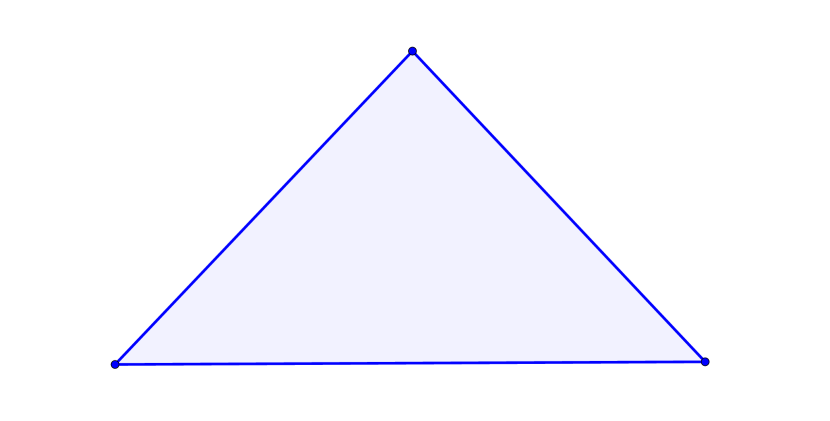
Figure 1: $G_{1}$

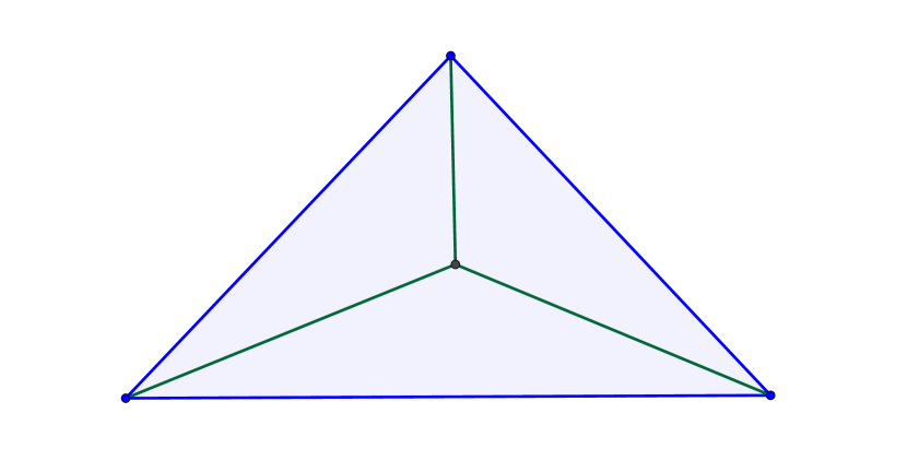
Figure 2: $G_{2}$

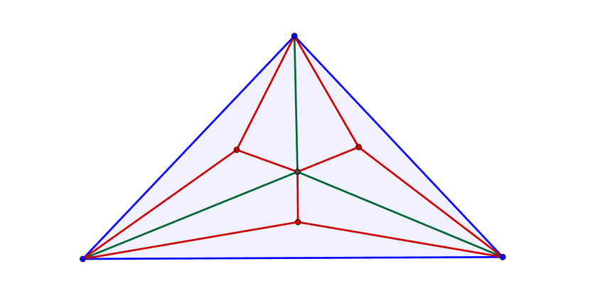
Figure 3: $G_{3}$

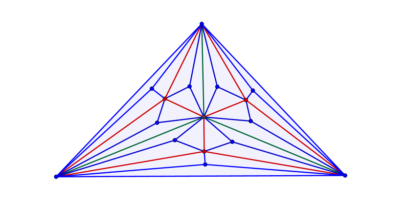
Figure 4: $G_{4}$

Before stating our main results, we record a few elementary facts based upon our construction of $G_{k}$ and observation of small cases:

Remark 1.1.

$|U_{1}|=3$, $|U_{k}|=3^{k-2}$ for $k>1$, and $\displaystyle|V(G_{k})|=\sum_{j=1}^{k}U_{j}=3+\sum_{j=0}^{k-2}3^{j}=\frac{3^{k-1}+5}{2}$.

Remark 1.2.

$\displaystyle|E(G_{k})|=3+\sum_{j=2}^{k}3|U_{j}|=3+\sum_{j=2}^{k}3^{j-1}=\frac{3^{k}+3}{2}$.

Remark 1.3.

Since every vertex in $V(G_{3})$ is adjacent to the single vertex in $U_{2}$, we know that $\gamma_{e}^{*}(G_{3})=1$.

Remark 1.4.

Let $S$ be any pair of vertices from $V(G_{2})$. Since every vertex in $V(G_{5})$ is adjacent to at least one of the vertices in $V(G_{2})$ and every pair of vertices in $V(G_{2})$ is adjacent, we know that every vertex of $V(G_{5})$ is within distance 2 of both vertices in $S$ and therefore $\gamma_{e}^{*}(G_{5})=2$. (See Figure 5.)

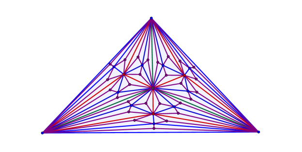
Figure 5: $G_{5}$

We further invite the reader to verify our observations and computations for the order, diameter, and porous exponential domination number of $G_{k}$ for $k\leq 7$, as presented in Table 1 below.

$k$	$|V(G_{k})|$	$|E(G_{k})|$	$diam(G_{k})$	$\gamma_{e}^{*}(G_{k})$
$1$	3	3	1	1
$2$	4	6	1	1
$3$	7	15	2	1
$4$	16	42	3	2
$5$	43	123	3	2
$6$	124	366	4	3
$7$	367	1095	5	3

Table 1: Observations for $G_{k}$, $k\leq 7$

2 Main Results

In Remark 1.4 we compute $\gamma_{e}^{*}(G_{5})=2$ by observation, but as $k$ increases, the number of vertices increases exponentially and $\gamma_{e}^{*}$ becomes increasingly difficult to compute by brute force. Thus, our main results in this paper are upper and lower bounds for $\gamma_{e}^{*}(G_{k})$. For all $k\geq 6$ we show that $U_{k-3}$ is a porous exponential dominating set for $G_{k}$, which proves the following:

Theorem 2.1.

For $k\geq 6$, $\gamma_{e}^{*}(G_{k})\leq 3^{k-5}$.

We can improve upon this bound for $k\geq 11$ by constructing a porous exponential dominating set using all of the vertices of a smaller Apollonian network rather than just a generation. In particular, we dominate $G_{k}$ with $V(G_{k-7})$ and prove the following:

Theorem 2.2.

For $k\geq 10$, $\gamma_{e}^{*}(G_{k})\leq\frac{3^{k-8}+5}{2}$.

To establish a lower bound, we apply a theorem from [3] that bounds $\gamma_{e}^{*}(G)$ from below in terms of $diam(G)$. In order to do this, we compute $diam(G_{k})$ for all $k$. This establishes the following:

Theorem 2.3.

For all $k\in\mathbb{N}$, $\gamma_{e}^{*}(G_{k})\geq$ $\left\lceil\frac{2k+5}{12}\right\rceil$.

Before we can prove these theorems, we need some basic results about Apollonian networks.

3 Apollonian Networks

All of the vertices in $G_{2}$ are adjacent to each other, but for larger values of $k$, the adjacencies are more restrictive. Recall that $x$ is a neighbor of $y$ in $G$ if $x$ is adjacent to $y$ in $G$, and the set of $y$’s neighbors in $G$ is the neighborhood of $y$ in $G$, denoted $N_{G}(y)$.

Lemma 3.1.

For all $k\geq 2$, and for every vertex $v$ in $U_{k}$,
(i) $v$ has no neighbor in $U_{k}$
(ii) $v$ has a neighbor in $U_{k-1}$
(iii) $v$ has exactly 3 distinct neighbors in $V(G_{k-1})$ and these vertices are also pairwise adjacent.
(iv) For all $r<k$ and for all $u\in U_{r}$, if $u$ is adjacent to $v$ then $|N_{G_{k}}(u)\cap N_{G_{k}}(v)|=2$.
(v) if $r<k$ and $v$ has more than one neighbor in $U_{r}$, then $r=1$

Proof.

Parts (i), (ii), and (iii) follow directly from the construction of $G_{k}$ because when a new vertex $v$ is added to $U_{k}$, it is made adjacent to a vertex $u$ of $U_{k-1}$ and two of $u$’s neighbors in $V(G_{k-1})$, say $n_{1}$ and $n_{2}$. By part (iii), if one of $v$’s neighbors is $u$, then the other two are neighbors of both $u$ and $v$, and (iv) follows. We prove (v) by contradiction. Suppose that $1<r<k$ and two of $u$, $n_{1}$, and $n_{2}$ are in $U_{r}$. We know that $u\in U_{k-1}$, so if $k-1=r>1$ then $n_{1},n_{2}\not\in U_{r}$ by part (i). If $1<r<k-1$ then it must be that $n_{1}$ and $n_{2}$ are the two vertices in $U_{r}$. But by the construction of $G_{k-1}$, all three of $u$’s neighbors in $G_{k-2}$ (including $n_{1}$ and $n_{2}$) must be adjacent. This contradicts (i) for $n_{1}\in U_{r}$ since $r>1$. ∎

Corollary 3.2.

For all $k\geq 4$ and for every vertex $v\in U_{k}$, $v$ has at least one neighbor in $V(G_{k-3})$.

Proof.

By Lemma 3.1 part (iii), $v$ has exactly 3 distinct neighbors in $V(G_{k-1})$, and these vertices are also pairwise adjacent. Denote these vertices by $n_{1}$, $n_{2}$, and $n_{3}$, and suppose that $n_{1}\in U_{r}$, $n_{2}\in U_{s}$, and $n_{3}\in U_{t}$, where $r\leq s\leq t\leq k-1$. Since $k\geq 4$, then $k-3\geq 1$ and if $r>k-3$ then by pigeonhole principle, two of $r$, $s$, and $t$ must be equal which contradicts Lemma 3.1 part (i). Therefore $r\leq k-3$ and $n_{1}\in V(G_{k-3})$. ∎

Given $k\in\mathbb{N}$, $r\leq k$, and $v\in U_{r}$, define $P_{k}(v)=\{\{x,y\}\mid x\in U_{k}\text{ and }v,x,\text{ and }y\text{ are pairwise adjacent}\}$. This is the set of pairs of vertices, at least one of which is from the $k$th generation, that form triangles with $v$ in $G_{k}$, the very same triangles that will anchor the $(k+1)$st generation of vertices. By the construction of $G_{k+1}$, there is a one-to-one corespondence between $P_{k}(v)$ and the $(k+1)$st generation neighbors of $v$. It follows that $|P_{k}(v)|=|N_{G_{k+1}}(V)\cap U_{k+1}|$, in other words the number of $(k+1)$st generation neighbors of $v$. The next lemma states that the number of such neighbors doubles with every generation.

Lemma 3.3.

For all $k\in\mathbb{N}$, for all $r\leq k$, and for all $v\in U_{r}$, $|P_{k+1}(v)|=2|P_{k}(v)|$.

Proof.

By the construction of $G_{k+1}$, there is a one-to-one corespondence between $P_{k}(v)$ and the $(k+1)$st generation neighbors of $v$. It follows that the members of $P_{k+1}(v)$ are precisely the pairs $\{z,x\}$ and $\{z,y\}$ where $z\in U_{k+1}\cap N_{G_{k+1}}(v)$ and $\{x,y\}\in P_{k}(v)$. ∎

Corollary 3.4.

For all $k\in\mathbb{N}$, for all $r\leq k$, and for all $v\in U_{r}$.

$$|P_{k}(v)|=\begin{cases}3(2^{k-r})&\text{ when $r>1$}\\ 2^{k-1}&\text{ when $r=1$}\end{cases}$$

Proof.

We proceed by induction on $k$. If $k=1$ then $r=1$, then indeed for all $v\in U_{1}$, $|P_{1}(v)|=1=2^{1-1}$. If $k>1$ and $r=1$ then, by Lemma 3.3, $|P_{k}(v)|=2|P_{k-1}(v)|=2(2^{k-2})=2^{k-1}$ by inductive hypothesis. If $k=2$ and $r=2$ then for the single vertex $v\in U_{2}$, $|P_{2}(v)|=3=3(2^{1-1})$. If $k>2$ and $r>1$ then, by Lemma 3.3, $|P_{k}(v)|=2|P_{k-1}(v)|=2(3(2^{(k-1)-r}))=3(2^{k-r})$ by inductive hypothesis. ∎

Corollary 3.5.

For all $k\geq 2$, and for all $v\in V(G_{k-1})$, $v$ has a neighbor in $U_{k}$.

Proof.

By the construction of $G_{k}$ there is a one-to-one corespondence between $P_{k-1}(v)$ and the $k$th generation neighbors of $v$. By Corollary 3.4 $|P_{k-1}(v)|$ is nonnegative, and therefore $v$ has a neighbor in $U_{k}$. ∎

Corollary 3.6.

For all $k\geq 2$, and for all $v\in V(G_{k})\setminus U_{k-1}$, $v$ has a neighbor in $U_{k-1}$.

Proof.

If $v\in U_{k}$ then the result follows immediately from Lemma 3.1 part (ii). If $v\in U_{r}$, where $r\leq k-2$ then the result follows from Corollary 3.5. ∎

Lemma 3.7.

For all $k\in\mathbb{N}$, for all $r\leq k$, and for all $v\in U_{r}$,

$$d_{G_{k}}(v)=\begin{cases}|P_{k}(v)|&\text{ when $r>1$}\\ |P_{k}(v)|+1&\text{ when $r=1$}\end{cases}$$

Proof.

By the construction of $G_{k+1}$, there is a one-to-one corespondence between $P_{k}(v)$ and the $(k+1)$st generation neighbors of $v$. It follows that for all $k\in\mathbb{N}$, for all $r\leq k$, and for all $v\in U_{r}$,

$$d_{G_{k+1}}(v)=d_{G_{k}}(v)+|P_{k}(v)|.$$

We now prove the lemma by induction on $k$. If $k=1$ then $r=1$ and $d_{G_{k}}(v)=2=1+1=|P_{k}(v)|+1$. If $k>1$ and $r=1$ then $d_{G_{k}}(v)=d_{G_{k-1}}(v)+|P_{k-1}(v)|=|P_{k-1}(v)|+1+|P_{k-1}(v)|=2|P_{k-1}(v)|+1=|P_{k}(v)|+1$ by inductive hypothesis and Lemma 3.3. If $k=2$ and $r=2$ then for the single vertex $v\in U_{2}$, $d_{G_{k}}(v)=3=|P_{k}(v)|$. If $k>2$ and $r>1$ then $d_{G_{k}}(v)=d_{G_{k-1}}(v)+|P_{k-1}(v)|=|P_{k-1}(v)|+|P_{k-1}(v)|=2|P_{k-1}(v)|=|P_{k}(v)|$ by inductive hypothesis and Lemma 3.3. ∎

Corollary 3.8.

For all $k\in\mathbb{N}$, for all $r\leq k$, and for all $v\in U_{r}$,

$$d_{G_{k}}(v)=\begin{cases}3(2^{k-r})&\text{ when $r>1$}\\ 2^{k-1}+1&\text{ when $r=1$}\end{cases}$$

Proof.

This follows immediately from Corollary 3.4 and Lemma 3.7. ∎

4 Upper Bounds for $\gamma_{e}^{*}$

In [3] the nonporous exponential dominating number of G, denoted $\gamma_{e}(G)$, is defined and the following theorem is proved:

Theorem 4.1.

(Dankelmann, et al) If G is a connected graph of order n, then $\gamma_{e}(G)\leq\frac{2}{5}(n+2)$.

This theorem, together with Remark 1.1 and the fact that $\gamma_{e}^{*}(G)\leq\gamma_{e}(G)$, immediately establishes the following corollary:

Corollary 4.2.

For all $k\in\mathbb{N}$, $\gamma_{e}^{*}(G_{k})\leq\frac{3^{k-1}+9}{5}$.

The recursive nature of our construction of $G_{k}$ makes it clear that for, $k>1$, $G_{k}$ can be conceived as a union of three copies of $G_{k-1}$. More precisely, if we consider the three triangles in $G_{2}$ that include the vertex in $U_{2}$, each could be the first generation of a copy of $G_{k-1}$. Together, these three copies of $G_{k-1}$ comprise a copy of $G_{k}$. This perspective is also discussed in [9]. The following lemma follows immediately from this construction.

Lemma 4.3.

For all $k\in\mathbb{N}$, $\gamma_{e}^{*}(G_{k+1})\leq 3\gamma_{e}^{*}(G_{k})$.

Corollary 4.4.

For $k\geq 5$, $\gamma_{e}^{*}(G_{k})\leq 2(3^{k-5})$.

Proof.

By induction on $k$. If $k=5$ then the result follows immediately from Remark 1.4. If $k>5$ then by Lemma 4.3, $\gamma_{e}^{*}(G_{k})\leq 3\gamma_{e}^{*}(G_{k-1})=3(2(3^{(k-1)-5}))=2(3^{k-5})$ by inductive hypothesis. ∎

We now establish a better upper bound by proving Theorem 2.1:

Proof.

Suppose $k\geq 6$. Let $S=U_{k-3}$ and compute $w_{S}^{*}(v)$ for all $v\in V(G_{k})$.

Case 1: Suppose $v\in V(G_{k-4})$. By Corollary 3.5, $v$ has a neighbor in $S$ and $w^{*}_{S}(v)\geq 1$.

Case 2: Suppose $v\in U_{k-3}$. Then $v\in S$ and $w^{*}_{S}(v)\geq 2$.

Case 3: Suppose $v\in U_{k-2}$. By Corollary 3.6, $v$ has a neighbor in $S$ and $w^{*}_{S}(v)\geq 1$.

Case 4: Suppose $v\in U_{k-1}$ or $v\in U_{k}$. By Lemma 3.1, $v$ has three distinct neighbors in $V(G_{k-1})$. If $v$ has a neighbor in $S$ then $w^{*}_{S}(v)\geq 1$. Otherwise, at least one of $v$’s neighbors is in $V(G_{k-4})$. Let $n$ be this vertex. By Corollary 3.4, $n$ has more than one neighbor in $S$. Therefore, $v$ is within distance 2 of at least two distinct vertices of $S$, and $w^{*}_{S}(v)\geq 1$.

We have shown that $S$ is a porous exponential dominating set for $G_{k}$. By Remark 1.1, $|S|=3^{k-5}$, and therefore $\gamma_{e}^{*}(G_{k})\leq 3^{k-5}$. ∎

We proved Theorem 2.1 by using a particular generation as a porous exponential dominating set. For $k\geq 10$, we can improve this upper bound by using the entire vertex set of a smaller Apollonian network as a dominating set. This is the strategy we employ in the proof of Theorem 2.2:

Proof.

Suppose $k\geq 10$. Let $S=V(G_{k-7})$ and compute $w_{S}^{*}(v)$ for all $v\in V(G_{k})$.

Case 1: Suppose $v\in U_{j}$, $j\leq k-4$. Then by Corollary 3.2, either $v\in S$ or $v$ has a neighbor in $S$. In both cases, $w^{*}_{S}(v)\geq 1$.

Case 2: Suppose $v\in U_{j}$, $k-3\leq j\leq k-2$. If $v$ has a neighbor in $S$, then $w^{*}_{S}(v)\geq 1$. Otherwise, by Corollary 3.2, $v$ has a neighbor $n$ in either $U_{k-5}$ or $U_{k-6}$. By Lemma 3.1, $n$ has at least two neighbors in $S$. Therefore, $v$ is within distance 2 of at least two distinct vertices of $S$, and $w^{*}_{S}(v)\geq 1$.

Case 3: Suppose $v\in U_{k-1}$. If $v$ has a neighbor in $S$, then $w^{*}_{S}(v)\geq 1$. Otherwise, by Corollary 3.2, $v$ has a neighbor $n$ in $U_{n-4}$, $U_{n-5}$, or $U_{n-6}$. By Corollary 3.2, $n$ has a neighbor $w\in S$. If $w\in U_{1}$ then $w$ has two neighbors $x,y\in U_{1}$. Note that $w,x,y\in S$, and that $v$ is within distance 2 of $w$ and within distance 3 of each of $x$ and $y$. Therefore $w^{*}_{S}(v)\geq\frac{1}{2}+\frac{1}{4}+\frac{1}{4}\geq 1$. Otherwise $w\in U_{j}$, $j\geq 2$, and by Lemma 3.1 $w$ has three distinct neighbors $x_{1},x_{2},x_{3}\in V(G_{j-1})$. Note that $w,x_{1},x_{2},x_{3}\in S$, and that $v$ is within distance 2 of $w$ and within distance 3 of each of $x_{1}$, $x_{2}$, and $x_{3}$. Therefore $w^{*}_{S}(v)\geq\frac{1}{2}+\frac{1}{4}+\frac{1}{4}+\frac{1}{4}\geq 1$.

Case 4: Suppose $v\in U_{k}$. If $v$ has a neighbor in $S$, then $w^{*}_{S}(v)\geq 1$. Otherwise, by Corollary 3.2, $v$ has a neighbor $n$ in $U_{n-3}$, $U_{n-4}$, $U_{n-5}$, or $U_{n-6}$. By Corollary 3.2, $n$ has a neighbor $w$ such that $w\in U_{k-6}$ or $w\in S$. If $w\in S$ then proceed as in Case 3. If $w\in U_{k-6}$ then by Lemma 3.1 $w$ has three distinct neighbors $x_{1},x_{2},x_{3}\in S$. Let $x_{3}$ be the neighbor with smallest generation. Since $k\geq 10$, by Corollary 3.4 and Lemma 3.1 part (v), $x_{3}$ has at least 3 neighbors $y_{1},y_{2},y_{3}\in U_{k-7}$ distinct from $x_{1}$ and $x_{2}$. Note that $x_{1},x_{2},x_{3},y_{1},y_{2},y_{3}\in S$. Also note that $v$ is within distance 3 of each of $x_{1}$, $x_{2}$, and $x_{3}$, and within distance 4 of each of $y_{1}$, $y_{2}$, and $y_{3}$. Therefore $w^{*}_{S}(v)\geq\frac{1}{4}+\frac{1}{4}+\frac{1}{4}+\frac{1}{8}+\frac{1}{8}+\frac{1}{8}\geq 1$.

We have shown that $S$ is a porous exponential dominating set for $G_{k}$. By Remark 1.1, $|S|=\frac{3^{k-8}+5}{2}$, and therefore $\gamma_{e}^{*}(G_{k})\leq\frac{3^{k-8}+5}{2}$. ∎

5 Lower Bound for $\gamma_{e}^{*}$

Recall that for a connected graph $G$, the diameter of $G$, denoted $diam(G)$, is the largest possible distance between a pair of vertices in $G$. In [3] the nonporous exponential domination number of $G$, denoted $\gamma_{e}(G)$, is defined and the following theorem is proven:

Theorem 5.1.

(Dankelmann, et al) If $G$ is a connected graph, then $\gamma_{e}(G)\geq\left\lceil\frac{diam(G)+2}{4}\right\rceil$.

In fact, the proof of this result in [3] is sufficient to establish the following lemma:

Lemma 5.2.

If $G$ is a connected graph, then $\gamma_{e}^{*}(G)\geq\left\lceil\frac{diam(G)+2}{4}\right\rceil$.

We now compute $diam(G_{k})$ for every Apollonian network $G_{k}$.

Lemma 5.3.

For all $k\in\mathbb{N}$, $diam(G_{k+3})\leq diam(G_{k})+2$.

Proof.

Suppose $x,y\in V(G_{k+3})$ and $d_{G_{k+3}}(x,y)=diam(G_{k+3})$. By Lemma 3.1 and Corollary 3.2, we know that $x$ and $y$ have neighbors $u$ and $v$, respectively, in $V(G_{k})$. It follows that

$$diam(G_{k+3})=d_{G_{k+3}}(x,y)\leq d_{G_{k}}(u,v)+2\leq diam(G_{k})+2.$$

∎

Corollary 5.4.

For all $k\in\mathbb{N}$, $diam(G_{k})\leq\left\lfloor{\frac{2k+1}{3}}\right\rfloor$.

Proof.

We proceed by induction on $k$ and show that $diam(G_{k})\leq\frac{2k+1}{3}$. For $k=1,2,3$, it is easy to verify that $diam(G_{k})=1,1,2$, respectively, and establish the desired result. For $k>3$, by Lemma 5.3, $diam(G_{k})\leq diam(G_{k-3})+2\leq\frac{2(k-3)+1}{3}+2=\frac{2k+1}{3}$, by inductive hypothesis. Since $diam(G_{k})$ is an integer, the result follows. ∎

Lemma 5.5.

For all $k\in\mathbb{N}$ there exists $x,y\in U_{k}$ such that $d_{G_{k}}(x,y)=diam(G_{k})$.

Proof.

First, observe that the statement is true for $k=1$, so we may assume $k\geq 2$. Let $u,v\in V(G_{k})$ such that $d_{G_{k}}(u,v)=diam(G_{k})$. If $u\in U_{k}$ then let $x=u$. Otherwise, by Corollary 3.5, there exists $x\in U_{k}$ such that $x$ is adjacent to $u$. If $v\in U_{k}$ then let $y=v$. Otherwise, by Corollary 3.5, there exists $y\in U_{k}$ such that $y$ is adjacent to $v$. Let $P$ be a shortest path joining $x$ and $y$. Let $w_{1}$ be the vertex adjacent to $x$ in $P$, and $w_{2}$ be the vertex adjacent to $y$ in $P$. By Lemma 3.1 part (iii), $u$ is adjacent to $w_{1}$ and $v$ is adjacent to $w_{2}$. Define $Q$ to be the path formed by replacing $x$ and $y$ in $P$ with $u$ and $v$. Then the length of $Q$ is the same as the length of $P$. Since $d_{G_{k}}(u,v)=diam(G_{k})$, this shows that the length of $P$ is at least $diam(G_{k})$. Since $P$ is a shortest path joining $x$ and $y$, $d_{G_{k}}(x,y)=diam(G_{k})$. ∎

Lemma 5.6.

For all $k\in\mathbb{N}$, $diam(G_{k+3})\geq diam(G_{k})+2$.

Proof.

The result is easily seen to be true for $k=1$, so we may assume that $k\geq 2$. (See Figure 4 and Table 1.) By Lemma 5.5, let $u,v\in V(G_{k})$ such that $d_{G_{k}}(u,v)=diam(G_{k})$. By Lemma 3.1, any path joining $u$ and $v$ must include vertices from $V(G_{k-1})$. By Corollary 3.5, $u$ has a neighbor $u_{1}$ in $U_{k+1}$. By the construction of $G_{k+2}$, $u$ and $u_{1}$ have a common neighbor $u_{2}$ in $U_{k+2}$. By the construction of $G_{k+3}$, $u$, $u_{1}$, and $u_{2}$ have a common neighbor $x$ in $U_{k+3}$. By Lemma 3.1, $u$, $u_{1}$, and $u_{2}$ are the only neighbors of $x$ in $G_{k+3}$. Therefore, $u$ has a neighbor $x\in U_{k+3}$ such that $N_{G_{k+3}}(x)\cap V(G_{k-1})=\emptyset$. An analogous argument shows that $v$ has a neighbor $y\in U_{k+3}$ such that $N_{G_{k+3}}(y)\cap V(G_{k-1})=\emptyset$. Note that any path joining $x$ and $y$ must include vertices from $V(G_{k-1})$ because otherwise we could construct a path joining $u$ and $v$ without such vertices, which contradicts our earlier claim to the contrary.

Let $P$ be a shortest path $x,w_{1},w_{2},\ldots,w_{m},y$ joining $x$ and $y$. Choose $i$ as small as possible and $j$ as large as possible such that $w_{i},w_{j}\in V(G_{k-1})\cap V(P)$. Since the only neighbors of $x$ are $u$, $u_{1}$, and $u_{2}$ then $w_{i}$ is adjacent to at least one of these. By the construction of $G_{k+1}$ and $G_{k+2}$, $u$ is adjacent to all of the neighbors of $u_{1}$ and $u_{2}$ in $V(G_{k-1})$, and therefore $u$ is adjacent to $w_{i}$. Analogously, $v$ is adjacent to $w_{j}$. Let $Q$ be the path $u,w_{i},w_{i+1},\ldots,w_{j-1},w_{j},v$ joining $u$ and $v$. Since $N_{G_{k+3}}(x)\cap V(G_{k-1})=\emptyset$ and $N_{G_{k+3}}(y)\cap V(G_{k-1})=\emptyset$, the length of $P$ is at least 2 more than the length of $Q$. It follows that the length of $P$ is at least $diam(G_{k})+2$. Since $P$ is a shortest length path joining $x$ and $y$, $diam(G_{k+3})\geq diam(G_{k})+2$. ∎

Together, Lemma 5.3 and Lemma 5.6 imply the following result which was stated in [8] with greater generality but without a complete proof.

Corollary 5.7.

For all $k\in\mathbb{N}$, $diam(G_{k+3})=diam(G_{k})+2$.

Corollary 5.8.

For all $k\in\mathbb{N}$, $diam(G_{k})\geq\left\lceil{\frac{2k-1}{3}}\right\rceil$.

Proof.

We proceed by induction on $k$ and show that $diam(G_{k})\geq\frac{2k-1}{3}$. For $k=1,2,3$, it is easy to verify that $diam(G_{k})=1,1,2$, respectively, and establish the desired result. For $k>3$, by Lemma 5.6, $diam(G_{k})\geq diam(G_{k-3})+2\geq\frac{2(k-3)-1}{3}+2=\frac{2k-1}{3}$, by inductive hypothesis. Since $diam(G_{k})$ is an integer, the result follows. ∎

Corollary 5.9.

For all $k\in\mathbb{N}$, $diam(G_{k})=\left\lceil{\frac{2k-1}{3}}\right\rceil$.

Proof.

This result follows easily from Corollary 5.4, Corollary 5.8, and the fact that $\left\lfloor{\frac{2k+1}{3}}\right\rfloor=\left\lceil{\frac{2k-1}{3}}\right\rceil$, which the reader can easily check by cases $k\equiv 0,1,2$ (mod 3). ∎

We can now prove Theorem 2.3:

Proof.

By Corollary 5.9, $diam(G_{k})=\left\lceil{\frac{2k-1}{3}}\right\rceil\geq{\frac{2k-1}{3}}$, and therefore $\frac{diam(G_{k})+2}{4}\geq\frac{2k+5}{12}$. By Lemma 5.2, $\gamma_{e}^{*}(G_{k})\geq\left\lceil\frac{diam(G_{k})+2}{4}\right\rceil\geq\left\lceil\frac{2k+5}{12}\right\rceil$. ∎

6 Acknowledgements

The authors would like to thank CURM, the Center for Undergraduate Research, for facilitating a wonderful undergraduate research experience and funding our research through NSF grant DMS-1148695. We would also like to thank Concord University for their encouragement and financial support.

References

- [1] M. Anderson, R. Brigham, J. Carrington, R. Vitray, J. Yellen, On Exponential Domination of , J. Graphs. Combin. 6 No. 3 (2009) 341-351.
- [2] J. Andrade, H. Herrmann, R. Andrade, L. Silva, Simultaneously Scale-Free, Small World, Euclidean, Space Filling, and with Matching Graphs, Phys. Rev. Lett. 94(1) (2005) 18702.
- [3] P. Dankelmann, D. Day, D. Erwin, S. Mukwembi, H. Swart, Domination with Exponential Decay, Discrete Math 309(19) (2009) 5877–5883.
- [4] J.P.K. Doye and C. Massen, Characterizing the network topology of the energy landscapes of atomic clusters J. Chem. Phys. 122 (2005) 84105.
- [5] T.W. Haynes, S.T. Hedetniemi, P.J. Slater, Domination in Graphs: Advanced Topics, Marcel Dekker, New York, 1998.
- [6] T.W. Haynes, S.T. Hedetniemi, P.J. Slater, Fundamentals of Domination in Graphs, Marcel Dekker, New York, 1998.
- [7] D. B. West, Introduction to Graph Theory, 2nd ed., Prentice Hall, 2000.
- [8] Z. Zhang, F. Comellas, G. Fertin, L. Rong, High Dimensional Apollonian Networks, J. Phys. A: Math. Gen. 39 (2006) 1811.
- [9] Z. Zhang, B. Wu, and F. Comellas, The Number of Spanning Trees in Apollonian Networks, Discrete Applied Mathematics. (to appear)