On the numerical solution of second order ordinary differential equations in the high-frequency regime

Abstract

We describe an algorithm for the numerical solution of second order linear ordinary differential equations in the high-frequency regime. It is founded on the recent observation that solutions of equations of this type can be accurately represented using nonoscillatory phase functions. Unlike standard solvers for ordinary differential equations, the running time of our algorithm is independent of the frequency of oscillation of the solutions. We illustrate this and other properties of the method with numerical experiments.

1 Introduction

Second order linear differential equations of the form

$$y^{\prime\prime}(t)+\lambda^{2}q(t)y(t)=0\ \ \ \mbox{for all}\ \ a\leq t\leq b$$ (1)

are ubiquitous in analysis and mathematical physics. As a consequence, much attention has been devoted to the development of numerical algorithms for their solution and, in most regimes, fast and accurate methods are available.

However, when $q$ is positive and $\lambda$ is real-valued and large, the solutions of (1) are highly oscillatory (this is a consequence of the Sturm comparison theorem) and standard solvers for ordinary differential equations (for instance, Runge-Kutta schemes and spectral methods) suffer. Specifically, their running times grow linearly with the parameter $\lambda$, which makes them prohibitively expensive when $\lambda$ is large.

Because of the poor performance of standard solvers, asymptotic methods are often used in this regime. In some instances, they allow for the accurate evaluation of solutions of equation of the form (1) using a number of operations which is independent of the parameter $\lambda$. For example, [3] presents an $\mathcal{O}(1)$ algorithm for calculating Legendre polynomials of arbitrary order using a combination of direct evaluation and asymptotic formulas; it achieves near machine precision accuracy and serves as the basis for an efficient parallel algorithm (also presented in [3]) for the construction of Gauss-Legendre quadratures of extremely large orders.

The formulas used in [3] are particular to Legendre polynomials, and while the same approach can be applied to other classes of special functions defined by equations of the form (1), in each case a new, specialized approach must be devised. Indeed, despite the extensive existing literature on the asymptotic approximation of Legendre polynomials, the algorithm of [3] required the development of a novel asymptotic expansion with suitable numerical properties.

Here, we describe an algorithm for the numerical solution of second order linear ordinary differential equations of the form (1) whose running time is independent of the parameter $\lambda$. It applies to a large class of second order ordinary differential equations — which includes those defining Bessel functions, Legendre functions of noninteger orders, prolate spheriodal wave functions and the classical orthogonal polynomials — and its only inputs are the parameter $\lambda$ and the values of the function $q$ at a collection of points on the interval $[a,b]$ on which (1) is given.

Our approach proceeds by constructing a nonscillatory phase function which represents solutions of (1). We say that $\alpha$ is a phase function for (1) if the functions $u,v$ defined by the formulas

$$u(t)=\frac{\cos(\alpha(t))}{\left|\alpha^{\prime}(t)\right|^{1/2}},$$ (2)

and

$$v(t)=\frac{\sin(\alpha(t))}{\left|\alpha^{\prime}(t)\right|^{1/2}}$$ (3)

comprise a basis in the space of solutions of (1). Phase functions play a key role in the theories of special functions and global transformations of ordinary differential equations [4, 19, 20, 1], and are the basis of many numerical algorithms (see [23, 11, 15] for representative examples).

It was observed by E.E. Kummer in [18] that $\alpha$ is a phase function for (1) if and only if it satisfies the third order nonlinear differential equation

$$\left(\alpha^{\prime}(t)\right)^{2}=\lambda^{2}q(t)-\frac{1}{2}\frac{\alpha^{\prime\prime\prime}(t)}{\alpha^{\prime}(t)}+\frac{3}{4}\left(\frac{\alpha^{\prime\prime}(t)}{\alpha^{\prime}(t)}\right)^{2}$$ (4)

on the interval $[a,b]$. The presence of quotients in (4) is often inconvenient, and we prefer the more tractable equation

$$r^{\prime\prime}(t)-\frac{1}{4}\left(r^{\prime}(t)\right)^{2}+4\lambda^{2}\left(\exp(r(t))-q(t)\right)=0$$ (5)

obtained from (4) by letting

$$\alpha^{\prime}(t)=\lambda\exp\left(\frac{r(t)}{2}\right).$$ (6)

Of course, if $r$ is a solution of (5) then a solution $\alpha$ of (4) is given by the formula

$$\alpha(t)=\lambda\int_{a}^{t}\exp\left(\frac{r(u)}{2}\right)\ du.$$ (7)

We will refer to (4) as Kummer’s equation and (5) as the logarithm form of Kummer’s equation. The form of these equations and the appearance of $\lambda$ in them suggests that their solutions will be oscillatory — and most of them are. However, there are several well-known examples of second order ordinary differential equations which admit nonoscillatory phase functions. For example, the function

$$\alpha(t)=\lambda\arccos(t)$$ (8)

is a phase function for Chebyshev’s equation

$$y^{\prime\prime}(t)+\left(\frac{2+t^{2}+4\lambda^{2}(1-t^{2})}{4(1-t^{2})^{2}}\right)y(t)=0\ \ \ \mbox{for all}\ \ -1\leq t\leq 1.$$ (9)

Its existence is the basis of the fast Chebyshev transform and several other widely used numerical algorithms (see, for instance, [25]). Bessel’s equation

$$y^{\prime\prime}(t)+\left(1-\frac{\lambda^{2}-1/4}{t^{2}}\right)y(t)=0\ \ \ \mbox{for all}\ \ 0<t<\infty$$ (10)

also admits a nonoscillatory phase function, although it cannot be expressed via elementary functions [15].

Exact solutions of (4) which are nonoscillatory need not exist in the general case. However, [14] and [5] make the observation that when the coefficient $q$ appearing in (1) is nonoscillatory, there exists a nonoscillatory function $\alpha$ such that (2), (3) approximate solutions (1) with accuracy on the order of $(\mu\lambda)^{-1}\exp(-\mu\lambda)$, where $\mu$ is a constant which depends on the coefficient $q$ but not on $\lambda$. More specifically, there is a nonoscillatory function $r$ which is a solution of the equation

$$r^{\prime\prime}(t)-\frac{1}{4}\left(r^{\prime}(t)\right)^{2}+4\lambda^{2}\left(\exp(r(t))-q(t)\right)=q(t)\nu,$$ (11)

where $\nu$ is a smooth function such that

$$\left\|\nu\right\|_{\infty}=\mathcal{O}\left(\frac{1}{\mu}\exp(-\mu\lambda)\right).$$ (12)

The function $\alpha$ obtained from $r$ via formula (7) is a solution of the nonlinear differential equation

$$\left(\alpha^{\prime}(t)\right)^{2}=\lambda^{2}\left(\frac{\nu(t)}{4\lambda^{2}}+1\right)q(t)-\frac{1}{2}\frac{\alpha^{\prime\prime\prime}(t)}{\alpha^{\prime}(t)}+\frac{3}{4}\left(\frac{\alpha^{\prime\prime}(t)}{\alpha^{\prime}(t)}\right)^{2}\ \ \ \mbox{for all}\ \ t\in\mathbb{R};$$ (13)

this implies that $\alpha$ is a phase function for the equation

$$y^{\prime\prime}(t)+\lambda^{2}\left(1+\frac{\nu(t)}{4\lambda^{2}}\right)q(t)y(t)=0\ \ \ \mbox{for all}\ \ a\leq t\leq b.$$ (14)

It follows from (14) and (12) that when $\alpha$ is inserted into formulas (2) and (3), the resulting functions approximate solutions of (1) with $\mathcal{O}\left((\mu\lambda)^{-1}\exp(-\mu\lambda)\right)$ accuracy (see Theorem 12 in [5]). The functions $r$ and $\alpha$ are nonoscillatory in the sense that then can be accurately represented using various series expansions (e.g., expansions in Chebyshev polynomials) whose number of terms does not depend on $\lambda$. In other words, $\mathcal{O}(1)$ terms are required to represent the solutions of (1) with $\mathcal{O}\left((\mu\lambda)^{-1}\exp(-\mu\lambda)\right)$ accuracy. This is an improvement over superasymptotic and hyperasymptotic expansions (see, for instance, [9, 8]), which represent solutions of (1) with accuracy on the order of $\exp(-\rho\lambda)$ using expansions with $\mathcal{O}(\lambda)$ terms. Theorem 12 of [5], which is reproduced as Theorem 87 in Section 9 of this article, gives a precise statement regarding the existence of nonoscillatory phase functions.

The method used to establish the existence of nonoscillatory phase functions in [5] is constructive and could serve as the basis of a numerical method for their computation. There are, however, at least two serious drawbacks to such an approach: an algorithm based on the method of [5] would require that the coefficient $q$ be extended to the real line as well as knowledge of the first two derivatives of $q$.

In this article, we describe a method for constructing a solution of the logarithm form of Kummer’s equation whose difference from the nonoscillatory solution of (11) is on the order of $\exp\left(-\frac{1}{2}\mu\lambda\right)$. It does not require that $q$ be extended beyond the interval $[a,b]$, nor does it take as input the values of the derivatives of $q$. Indeed, its only inputs are the parameter $\lambda$ and the values of $q$ at a collection of points on the interval $[a,b]$.

Our approach is based on two observations. First, that if

$$q(t)=1+\epsilon(t)$$ (15)

for all $t$ in an interval of the form $[a,a+\tau]$, where $\tau>0$ and $\epsilon$ is a smooth function of sufficiently small magnitude, then the difference between the solution of the boundary value problem

$$\left\{\begin{aligned} r^{\prime\prime}(t)-\frac{1}{4}\left(r^{\prime}(t)\right)^{2}+4\lambda^{2}\left(\exp(r(t))-q(t)\right)&=0\ \ \mbox{for all}\ \ a\leq t\leq b\\ r(a)=r^{\prime}(a)&=0\end{aligned}\right.$$ (16)

and the nonoscillatory solution of (11) is on the order of $\exp\left(-\frac{1}{2}\mu\lambda\right)$ on the interval $[a,b]$. Second, that when the coefficient $q$ is perturbed by a smooth function $\varphi$ which is of sufficiently small magnitude on the interval $[a,b]$, the changes induced in the restrictions of the nonoscillatory solution of (11) and its derivative to the interval $[a,b]$ are on the order of $\exp\left(-\mu\lambda\right)$. Both of these observations are obtained by combining Theorem 14 of Section 3.3 and Theorem 17 of Section 3, which are the two principal results of this article.

We exploit these observations as follows. First, we construct a windowed version $\tilde{q}$ of the function $q$ such that

$$\tilde{q}(t)=\begin{cases}1+\epsilon(t)&\mbox{for all}\ \ a\leq t\leq b-\Delta\\ q(t)&\mbox{for all}\ \ b-\Delta<t\leq b,\end{cases}$$ (17)

where $\Delta$ is a small positive real number and $\epsilon(t)$ is a function of small magnitude, and calculate a solution $r_{1}$ of the initial value problem

$$\left\{\begin{aligned} r_{1}^{\prime\prime}(t)-\frac{1}{4}\left(r_{1}^{\prime}(t)\right)^{2}+4\lambda^{2}\left(\exp\left(r_{1}(t)\right)-\tilde{q}(t)\right)&=0\ \ \ \mbox{for all}\ \ a\leq t\leq b\\ r_{1}(a)=r_{1}^{\prime}(a)&=0.\end{aligned}\right.$$ (18)

Next, we obtain a solution $r_{2}$ of the problem

$$\left\{\begin{aligned} r_{2}^{\prime\prime}(t)-\frac{1}{4}\left(r_{2}^{\prime}(t)\right)^{2}+4\lambda^{2}\left(\exp\left(r_{2}(t)\right)-q(t)\right)&=0\ \ \ \mbox{for all}\ \ a\leq t\leq b\\ r_{2}\left(b\right)=r_{1}\left(b\right)\ \ \ \mbox{and}\ \ \ r_{2}^{\prime}\left(b\right)&=r_{1}\left(b\right).\end{aligned}\right.$$ (19)

From our first observation, we see that the difference between the solution of (18) and the nonoscillatory function $\tilde{r}$ obtained by applying Theorem 87 to the equation

$$\tilde{r}^{\prime\prime}(t)-\frac{1}{4}\left(\tilde{r}^{\prime}(t)\right)^{2}+4\lambda^{2}\left(\exp(\tilde{r}(t))-\tilde{q}(t)\right)=0,$$ (20)

is on the order of $\exp\left(-\frac{1}{2}\mu\lambda\right)$. Moreover, according to our second observation, the difference between the the function $r_{1}$ and the nonoscillatory solution $r$ of

$$r^{\prime\prime}(t)-\frac{1}{4}\left(r^{\prime}(t)\right)^{2}+4\lambda^{2}\left(\exp(r(t))-q(t)\right)=q(t)\nu(t)$$ (21)

whose existence is guaranteed by Theorem 87 is on the order of

$$\exp\left(-\frac{1}{2}\mu\lambda\right)$$ (22)

on the interval $\left[b-\Delta,b\right]$, as is the difference between the derivatives of these two functions. In particular,

$$\left|r_{1}\left(b\right)-r\left(b\right)\right|+\left|r_{1}^{\prime}\left(b\right)-r^{\prime}\left(b\right)\right|=O\left(\exp\left(-\frac{1}{2}\mu\lambda\right)\right).$$ (23)

Together (12), (19), (21), and (23) imply that

$$\left|r_{2}(t)-r(t)\right|=O\left(\exp\left(-\frac{1}{2}\mu\lambda\right)\right)$$ (24)

for all $t\in[a,b]$. That is, the difference between the solution $r_{2}$ of the boundary value problem (19) and the nonoscillatory solution $r$ of (11) decays exponentially with $\lambda$.

In the high-frequency regime, the difference between $r_{1}$ and the nonoscillatory function $\tilde{r}$ is considerably smaller than machine precision, as is the difference between $r_{2}$ and the nonoscillatory function $r$. Consequently, for the purposes of numerical computation, $r_{1}$ and $r_{2}$ can be regarded as nonoscillatory. In particular, solutions of the boundary value problems (18) and (19) can be obtained via a standard method for the numerical solution of ordinary differential equations, and each of the functions $r_{1}$ and $r_{2}$ can be approximated to high accuracy by a finite series expansion whose number of terms does not depend on $\lambda$. Moreover, the number of operations required to compute these expansions of $r_{1}$ and $r_{2}$ does not depend on $\lambda$.

There is one significant limitation on the accuracy obtained by the algorithm of this paper. When $\lambda$ is large, the evaluation of the functions $u$, $v$ defined via the formulas (2) and (3) requires the computation of trigonometric functions of large arguments. There is an inevitable loss of accuracy when these calculations are performed in finite precision arithmetic. Nonetheless, acceptable accuracy is obtained in many cases. For instance, Section 5.3 describes an experiment in which the Bessel function of the first kind of order $10^{8}$ was evaluated at a large collection of points on the real axis to approximately ten digits of accuracy.

We also note that while some accuracy is lost when evaluating solutions of (1) when $\lambda$ is large, the phase functions produced by the algorithm of this paper are highly accurate is all cases. Among other things, they can be used to rapidly calculate the roots of special functions to extremely high precision. This and other applications of nonoscillatory phase functions will be reported at a later date.

The remainder of this paper is organized as follows. Section 2.8 summarizes a number of mathematical and numerical facts to be used in the rest of the paper. In Section 3, we develop the analytic apparatus used in Section 4 to develop an algorithm for the rapid solutions of second order linear differential equations in the high-frequency regime. Section 5.5 presents the results of numerical experiments conducted to assess the performance of the algorithm of Section 4.

2 Analytic and numerical preliminaries

2.1 Schwartz functions and tempered distributions

We say that an infinitely differentiable function $\varphi:\mathbb{R}\to\mathbb{C}$ is a Schwartz function if $\varphi$ and all of its derivatives decay faster than any polynomial. That is, if

$$\sup_{t\in\mathbb{R}}|t^{i}\varphi^{(j)}(t)|<\infty$$ (25)

for all pairs $i,j$ of nonnegative integers. The set of all Schwartz functions is denoted by $S(\mathbb{R})$. We endow it with the topology generated by the family of seminorms

$$\|\varphi\|_{k}=\sum_{j=0}^{k}\ \sup_{t\in\mathbb{R}}\left|t^{k}\varphi^{(j)}(x)\right|\ \ \ k=0,1,2,\ldots,$$ (26)

so that a sequence $\{\varphi_{n}\}$ of functions in $S(\mathbb{R})$ converges to $\varphi$ in $S(\mathbb{R})$ if and only if

$$\lim_{n\to\infty}\|\varphi_{n}-\varphi\|_{k}=0\ \ \ \mbox{for all}\ \ k=0,1,2,\ldots.$$ (27)

We denote the space of continuous linear functionals on $S(\mathbb{R})$, which are known as tempered distributions, by $S^{\prime}(\mathbb{R})$.

See, for instance, [16] for a thorough discussion of Schwartz functions and tempered distributions.

2.2 The Fourier transform

We define the Fourier transform of a function $f\in S(\mathbb{R})$ via the formula

$$\widehat{f}(\xi)=\int_{-\infty}^{\infty}\exp(-ix\xi)f(x)\ dx.$$ (28)

The Fourier transform is an isomorphism $S(\mathbb{R})\to S(\mathbb{R})$ (meaning that it is a continuous, invertible mapping $S(\mathbb{R})\to S(\mathbb{R})$ whose inverse is also continuous). The formula

$$\left<\widehat{\omega},\varphi\right>=\left<\omega,\widehat{\varphi}\right>$$ (29)

extends the Fourier transform to an isomorphism $S^{\prime}(\mathbb{R})\to S^{\prime}(\mathbb{R})$. The definition (29) coincides with (28) when $f\in L^{1}\left(\mathbb{R}\right)$. Moreover, when $f\in L^{2}\left(\mathbb{R}\right)$,

$$\widehat{f}(\xi)=\lim_{R\to\infty}\int_{-R}^{R}\exp(-ix\xi)f(x)\ dx.$$ (30)

Owing to our choice of convention for the Fourier transform,

$$\widehat{f*g}(\xi)=\widehat{f}(\xi)\widehat{g}(\xi)$$ (31)

and

$$\widehat{f\cdot g}(\xi)=\frac{1}{2\pi}\int_{-\infty}^{\infty}\widehat{f}(\xi-\eta)\widehat{g}(\eta)\ d\eta$$ (32)

whenever $f$ and $g$ are elements of $L^{1}\left(\mathbb{R}\right)$. Moreover,

$$f(x)=\frac{1}{2\pi}\int_{-\infty}^{\infty}\exp(ix\xi)\widehat{f}(\xi)\ d\xi$$ (33)

whenever $f$ and $\widehat{f}$ are elements of $L^{1}\left(\mathbb{R}\right)$. The observation that $f$ is an entire function when $\widehat{f}$ is a compactly supported distribution is one consequence of the well-known Paley-Wiener theorem. See [12, 13] for a thorough treatment of the Fourier transform.

2.3 The constant coefficient Helmholtz equation

The following theorem is a special case of a more general one which can be found in [17].

Theorem 1.

Suppose that $f\in S(\mathbb{R})$. If $\lambda$ is a positive real number, then the function $g$ defined by the formula

$$g(x)=\frac{1}{2\lambda}\int_{-\infty}^{\infty}\sin\left(\lambda\left|x-y\right|\right)f(y)\ dy$$ (34)

is an infinitely differentiable function,

$$g^{\prime\prime}(x)+\lambda^{2}g(x)=f(x)\ \ \mbox{for all}\ x\in\mathbb{R},$$ (35)

and

$$\widehat{g}(\xi)=\frac{\widehat{f}(\xi)}{\lambda^{2}-\xi^{2}}.$$ (36)

If $\lambda$ is complex number with positive imaginary part, then the function $h$ defined by the formula

$$h(x)=\frac{1}{2\lambda i}\int_{-\infty}^{\infty}\exp\left(2\lambda i\left|x-y\right|\right)f(y)\ dy$$ (37)

is an infinitely differentiable function,

$$h^{\prime\prime}(x)+\lambda^{2}h(x)=f(x)\ \ \mbox{for all}\ x\in\mathbb{R},$$ (38)

and

$$\widehat{h}(\xi)=\frac{\widehat{f}(\xi)}{\lambda^{2}-\xi^{2}}.$$ (39)

We interpret the Fourier transform (36) of $g$ as a tempered distribution defined via principal value integrals; that is to say that for all $\varphi\in S(\mathbb{R})$,

$$\left<\frac{\widehat{f}(\xi)}{\lambda^{2}-\xi^{2}},\varphi\right>=\frac{1}{2\lambda}\left(\lim_{\epsilon\to 0}\int_{|\xi-\lambda|>\epsilon}\frac{\widehat{f}(\xi)\varphi(\xi)}{\lambda-\xi}\ d\xi-\lim_{\epsilon\to 0}\int_{|\xi+\lambda|>\epsilon}\frac{\widehat{f}(\xi)\varphi(\xi)}{\lambda+\xi}\ d\xi\right).$$ (40)

The following variant of Theorem 1 can be found in [6].

Theorem 2.

Suppose that $f$ is continuous on the interval $[a,b]$, and that $\lambda$ is a positive real number. Suppose also that $y:[a,b]\to\mathbb{C}$ is twice continuously differentiable, and that

$$y^{\prime\prime}(x)+\lambda^{2}y(x)=f(x)\ \ \ \mbox{for all}\ \ a\leq x\leq b.$$ (41)

Then

$$y(x)=y(a)+y^{\prime}(a)(x-a)+\frac{1}{\lambda}\int_{a}^{x}\sin\left(\lambda\left(x-u\right)\right)f(u)\ du\ \ \ \ \mbox{for all}\ \ a\leq x\leq b.$$ (42)

2.4 Schwarzian derivatives

The Schwarzian derivative of a smooth function $f:\mathbb{R}\to\mathbb{R}$ is

$$\{f,t\}=\frac{f^{\prime\prime\prime}(t)}{f^{\prime}(t)}-\frac{3}{2}\left(\frac{f^{\prime\prime}(t)}{f^{\prime}(t)}\right)^{2}.$$ (43)

The Schwarzian derivative of $x(t)$ is related to the Schwarzian derivative of its inverse $t(x)$ through the formula

$$\{x,t\}=-\left(\frac{dx}{dt}\right)^{2}\{t,x\}.$$ (44)

This identity can be found, for instance, in Section 1.13 of [20].

2.5 Gronwall’s inequality

The following well-known inequality can be found in, for instance, [2].

Theorem 3.

Suppose that $f$ and $g$ are continuous functions on the interval $[a,b]$ such that

$$f(t)\geq 0\ \ \mbox{and}\ \ g(t)\geq 0\ \ \ \mbox{for all}\ \ a\leq t\leq b.$$ (45)

Suppose further that there exists a real number $C>0$ such that

$$f(t)\leq C+\int_{a}^{t}f(s)g(s)\ ds\ \ \ \mbox{for all}\ \ a\leq t\leq b.$$ (46)

Then

$$f(t)\leq C\exp\left(\int_{a}^{t}g(s)\ ds\right)\ \ \ \mbox{for all}\ \ a\leq t\leq b.$$ (47)

2.6 The Lambert $W$ function

The Lambert $W$ function or product logarithm is the multiple-valued inverse of the function

$$f(z)=z\exp(z).$$ (48)

We follow [7] in using $W_{0}$ to denote the branch of $W$ which is real-valued and greater than or equal to $-1$ on the interval $[-1/e,\infty)$. The following elementary fact concerning $W_{0}$ can be found in [7].

Theorem 4.

Suppose that $y\geq-1/e$ is a real number. Then

$$x\exp(x)\leq y\ \ \ \mbox{if and only if}\ \ \ x\leq W_{0}(y).$$ (49)

2.7 The Picard-Lindelöf Theorem

The following well-known theorem can be found in [6], among many other sources.

Theorem 5.

Suppose that $\Omega$ is a domain in $\mathbb{R}^{n}$, that the function $f:[t_{0},t_{1}]\times\Omega\to\mathbb{R}^{n}$ is continuous, and that there exists a $M$ such that

$$\left|f(t,x)-f(t,y)\right|\leq M|x-y|$$ (50)

for all $x,y\in\Omega$ and $t\in[t_{0},t_{1}]$. Suppose also that $t_{0}\leq t\leq t_{1}$, and that $y_{0}$ is an element of $\Omega$. Then there exist a positive real number $\epsilon$, and a differentiable function $y:[t_{0},t_{0}+\epsilon]\to\mathbb{C}$ such that

$$y^{\prime}(t)=f(t,y(t))\ \ \ \mbox{for all}\ \ t_{0}\leq t\leq t_{0}+\epsilon,$$ (51)

and $y(t_{0})=y_{0}$.

2.8 Chebyshev polynomials and interpolation

The $(m+1)$-point Chebyshev grid on the interval $[-1,1]$ is the set

$$\left\{\cos\left(\frac{\pi j}{m}\right):\ \ j=0,1,\ldots,m\right\}.$$ (52)

We refer to each element of (52) as a Chebyshev node or point.

Suppose that $f:[-1,1]\to\mathbb{R}$ is a Lipschitz continuous function. For each integer $m$, there exists a unique polynomial of degree $m$ which agrees with $f$ on the $(m+1)$-point Chebyshev grid. We refer to this polynomial as the $m^{th}$ order Chebyshev interpolant for $f$ and denote it by $\Psi_{m}\left[f\right]$. In other words, $\Psi_{m}\left[f\right]$ is the polynomial of degree $m$ defined by the requirement that

$$\Psi_{m}\left[f\right]\left(\cos\left(\frac{\pi j}{m}\right)\right)=f\left(\cos\left(\frac{\pi j}{m}\right)\right)$$ (53)

for $j=0,1,2,\ldots,m$. Moreover, $\Psi_{m}\left[f\right]$ converges to $f$ in $L^{\infty}\left(\left[-1,1\right]\right)$ norm as $m\to\infty$. The following two theorems provide estimates on the rate of convergence of $\Psi_{m}\left[f\right]$ in $L^{\infty}\left(\left[-1,1\right]\right)$ under additional assumptions on the function $f$. The observation that $\Psi_{m}\left[f\right]\to f$ when $f$ is Lipschitz continuous and proofs of the following two theorems can be found in [25], among many other sources.

Theorem 6.

Suppose that $p$ is a positive integer and $f\in C^{p}\left(\left[-1,1\right]\right)$. Then

$$\left\|\Psi_{m}\left[f\right]-f\right\|_{\infty}=O\left(m^{-p}\right).$$ (54)

Theorem 7.

Suppose that $f$ is analytic on an ellipse with foci $\pm 1$ the sum of whose semiaxes is $\rho$. Then

$$\left\|\Psi_{m}\left[f\right]-f\right\|_{\infty}=O\left(\rho^{-m}\right).$$ (55)

Given the values of $f$ on the $(m+1)$-point Chebyshev grid $x_{0},x_{1},\ldots,x_{m}$, the value of $\Psi\left[f\right]$ can be calculated at any point $x$ in $[-1,1]$ via the formula

$$\Psi\left[f\right](x)=\left(\sum_{j=0}^{m}\frac{(-1)^{j}f(x_{j})}{x-x_{j}}\right)\Big{/}\left(\sum_{j=0}^{m}\frac{(-1)^{j}}{x-x_{j}}\right).$$ (56)

The process of approximating a function $f$ via $\Phi\left[f\right]$ is referred to as Chebyshev interpolation and (56) is known as the barycentric interpolation formula for Chebyshev polynomials. The stability of barycentric interpolation is discussed extensively in [25].

Suppose that $f:[-1,1]\to\mathbb{R}$ is continuous function, that $m$ is a positive integer, and that $g$ is the function defined by the formula

$$g(t)=\int_{-1}^{t}\Psi_{m}\left[f\right](u)\ du.$$ (57)

If $\alpha=\{\alpha_{0},\alpha_{1},\ldots,\alpha_{m}\}$ is the vector defined by the formula

$$\alpha_{j}=f\left(\cos\left(\frac{\pi j}{m}\right)\right)$$ (58)

and $\beta=\{\beta_{0},\beta_{1},\ldots,\beta_{m}\}$ is the vector defined by the formula

$$\beta_{j}=g\left(\cos\left(\frac{\pi j}{m}\right)\right),$$ (59)

then we refer to the $(m+1)\times(m+1)$ matrix $S_{m}$ such that

$$S_{m}\alpha=\beta$$ (60)

as the spectral integration matrix of order $m$ (that such a matrix exists is clear since the underlying operation is linear).

The preceding constructions can be easily modified in order to accommodate functions defined on any finite interval $[a,b]$. For instance, if we denote the points in the $(m+1)$-point Chebyshev grid on $[-1,1]$ by $\rho_{0},\rho_{1},\ldots,\rho_{m}$, then the $(m+1)$-point Chebyshev grid on the interval $[a,b]$ is the set

$$\left\{\frac{a-b}{2}\ \rho_{j}+\frac{a+b}{2}:\ j=0,1\ldots,m.\right\}$$ (61)

Remark 1.

The set (52) is the collection of the extreme points of the $m^{th}$ order Chebyshev polynomial $T_{m}$. The roots of Chebyshev polynomials are often used as interpolation nodes instead. There are few meaningful differences between these two choices, although (52) includes the endpoints $\pm 1$, which is convenient when solving boundary value problems for ordinary differential equations.

3 Analytical apparatus

Here we develop the analytic apparatus used in Section 4 to design an algorithm for the numerical solution of second order linear ordinary differential equations of the form (1) whose running time is independent of the parameter $\lambda$.

In Section 3.1, we reformulate Kummer’s equation as a nonlinear integral equation in preparation for a statement of the main theorem of [5]. This is done in Section 9, and several consequences of this result are discussed there. In Section 3.3, we develop a theorem which bounds the restriction of the solution $r$ of the logarithm form of Kummer’s equation to an interval of the form $(-\infty,x_{0}]$ under the assumption that the coefficient $q$ is nearly equal to $1$ there. This result is recorded as Theorem 14. In Section 3, we use standard techniques from the theory of ordinary differential equations in order to bound the change in the solution of the logarithm form of Kummer’s equation when the initial conditions and coefficient $q$ are perturbed.

3.1 Integral equation formulation of Kummer’s equation

In this section, we reformulate Kummer’s equation

$$\left(\alpha^{\prime}(t)\right)^{2}=\lambda^{2}q(t)-\frac{1}{2}\frac{\alpha^{\prime\prime\prime}(t)}{\alpha^{\prime}(t)}+\frac{3}{4}\left(\frac{\alpha^{\prime\prime}(t)}{\alpha^{\prime}(t)}\right)^{2}$$ (62)

as a nonlinear integral equation in preparation for the statement of the principal result of [5]. We assume that the function $q$ has been extended to the real line.

By letting

$$\alpha^{\prime}(t)=\lambda\exp\left(\frac{r(t)}{2}\right)$$ (63)

in (62) we obtain

$$r^{\prime\prime}(t)-\frac{1}{4}\left(r^{\prime}(t)\right)^{2}+4\lambda^{2}\left(\exp(r(t))-q(t)\right)=0,$$ (64)

which we refer to as the logarithm form of Kummer’s equation. Representing the solution $r$ of (64) in the form

$$r(t)=\log(q(t))+\delta(t)$$ (65)

results in the equation

$$\delta^{\prime\prime}(t)-\frac{1}{2}\frac{q^{\prime}(t)}{q(t)}\delta^{\prime}(t)-\frac{1}{4}\left(\delta^{\prime}(t)\right)^{2}+4\lambda^{2}q(t)\left(\exp(\delta(t)-1)\right)=q(t)p(t),$$ (66)

where the function $p$ is defined by the formula

$$p(t)=\frac{1}{q(t)}\left(\frac{5}{4}\left(\frac{q^{\prime}(t)}{q(t)}\right)^{2}-\frac{q^{\prime\prime}(t)}{q(t)}\right).$$ (67)

By expanding the exponential in (66) in a power series and rearranging terms we obtain

$$\delta^{\prime\prime}(t)-\frac{1}{2}\frac{q^{\prime}(t)}{q(t)}\delta^{\prime}(t)+4\lambda^{2}q(t)\delta(t)-\frac{1}{4}\left(\delta^{\prime}(t)\right)^{2}+4\lambda^{2}q(t)\left(\frac{\left(\delta(t)\right)^{2}}{2!}+\frac{\left(\delta(t)\right)^{3}}{3!}+\cdots\right)=q(t)p(t).$$ (68)

The change of variables

$$x(t)=\int_{a}^{t}\sqrt{q(u)}\ du$$ (69)

transforms (68) into

$$\delta^{\prime\prime}(x)+4\lambda^{2}\delta(x)=S\left[\delta\right](x)+p(x),$$ (70)

where $S$ is the nonlinear differential operator defined via the formula

$$S\left[f\right](x)=\frac{\left(f^{\prime}(x)\right)^{2}}{4}-4\lambda^{2}\left(\frac{\left(f(x)\right)^{2}}{2!}+\frac{\left(f(x)\right)^{3}}{3!}+\cdots\right).$$ (71)

We observe that the function $p(t)$ defined in formula (67) is related to the Schwarzian derivative (see Section 2.4) $\{x,t\}$ of the function $x$ defined in (69) via the formula

$$p(t)=-\frac{2}{q(t)}\{x,t\}=-2\left(\frac{dt}{dx}\right)^{2}\{x,t\}.$$ (72)

From (72) and Formula (44) in Section 2.4, we see that

$$p(x)=2\{t,x\};$$ (73)

that is the function $p(x)$ is twice the Schwarzian derivative of the inverse of the function $x(t)$.

We also observe that the differential operator appearing on the left-hand side of (70) is the constant coefficient Helmholtz equation. In order to exploit this observation, we define the operator $T$ for functions $f\in S(\mathbb{R})$ via the formula

$$T\left[f\right](x)=\frac{1}{4\lambda}\int_{-\infty}^{\infty}\sin\left(2\lambda\left|x-y\right|\right)f(y)\ dy\ \ \ \mbox{for all}\ \ x\in\mathbb{R}.$$ (74)

According to Theorem 1, $T\left[f\right]$ is the unique solution of the ordinary differential equation

$$y^{\prime\prime}(x)+4\lambda^{2}y(x)=f(x)$$ (75)

such that

$$\widehat{T\left[f\right]}(\xi)=\frac{\widehat{f}(\xi)}{4\lambda^{2}-\xi^{2}}.$$ (76)

Consequently, introducing the representation

$$\delta(x)=T\left[\sigma\right](x)$$ (77)

into (70) results in the nonlinear integral equation

$$\sigma(x)=S\left[T\left[\sigma\right]\right](x)+p(x).$$ (78)

3.2 Nonoscillatory solutions of Kummer’s equation

Equation (78) does not admit solutions for all functions $p$. However, according to the following result, which appears as Theorem 12 in [5], if the function $p$ is nonoscillatory then there exists a function $\nu$ of small magnitude such that the nonlinear integral equation

$$\sigma(x)=S\left[T\left[\sigma\right]\right]+p(x)+\nu(x)$$ (79)

admits a solution $\sigma$ which is also nonoscillatory.

Theorem 8.

Suppose that $q\in C^{\infty}\left(\mathbb{R}\right)$ is strictly positive, that $x(t)$ is defined by the formula

$$x(t)=\int_{0}^{t}\sqrt{q(u)}\ du,$$ (80)

and that the function $p$ defined via the formula

$$p(x)=2\{t,x\}$$ (81)

is an element of $S(\mathbb{R})$. Suppose further that there exist positive real numbers $\lambda$, $\Gamma$ and $\mu$ such that

$$\lambda\geq 4\max\left\{\frac{1}{\mu},\Gamma\right\}$$ (82)

and

$$\left|\widehat{p}(\xi)\right|\leq\Gamma\exp\left(-\mu\left|\xi\right|\right)\ \ \ \mbox{for all}\ \ \xi\in\mathbb{R}.$$ (83)

Then there exist functions $\sigma$ and $\nu$ in $S(\mathbb{R})$ such that $\sigma$ is a solution of the nonlinear integral equation

$$\sigma(x)=S\left[T\left[\sigma\right]\right](x)+p(x)+\nu(x),\ \ \ \mbox{for all}\ \ x\in\mathbb{R},$$ (84)

$$\left|\widehat{\sigma}(\xi)\right|\leq\frac{3}{2\Gamma}\exp\left(-\mu|\xi|\right)\ \ \ \mbox{for all}\ \ \left|\xi\right|\leq\sqrt{2}\lambda,$$ (85)

$$\widehat{\sigma}(\xi)=0\ \ \ \mbox{for all}\ \ \left|\xi\right|>\sqrt{2}\lambda,$$ (86)

and

$$\|\nu\|_{\infty}\leq\frac{\Gamma}{\mu}\exp\left(-\mu\lambda\right).$$ (87)

Suppose that $\sigma$ and $\nu$ are the functions obtained by invoking Theorem 87, and that $x(t)$ is the function defined by the formula

$$x(t)=\int_{a}^{t}\sqrt{q(u)}\ du.$$ (88)

We define $\delta$ by the formula

$$\delta(x)=T\left[\sigma\right](x),$$ (89)

$r$ by the formula

$$r(t)=\log(q(t))+\delta(x(t)),$$ (90)

and $\alpha$ by the formula

$$\alpha(t)=\lambda\int_{a}^{t}\exp\left(\frac{r(u)}{2}\right)\ du.$$ (91)

From the discussion in Section 3.1, we conclude that $\delta(x)$ is a solution of the nonlinear differential equation

$$\delta^{\prime\prime}(x)+4\lambda^{2}\delta(x)=S\left[\delta\right](x)+p(x)+\nu(x)\ \ \ \mbox{for all}\ \ x\in\mathbb{R},$$ (92)

that $\delta(x(t))$ is a solution of the nonlinear differential equation

$$\delta^{\prime\prime}(t)-\frac{1}{2}\frac{q^{\prime}(t)}{q(t)}\delta^{\prime}(t)-\frac{1}{4}\left(\delta^{\prime}(t)\right)^{2}+4\lambda^{2}q(t)\left(\exp(\delta(t))-1\right)=q(t)\left(p(t)+\nu(t)\right)\ \ \ \mbox{for all}\ \ \ t\in\mathbb{R},$$ (93)

that $r(t)$ is a solution of the nonlinear differential equation

$$r^{\prime\prime}(t)-\frac{1}{4}(r^{\prime}(t))^{2}+4\lambda^{2}\left(\exp(r(t))-q(t)\right)=q(t)\nu(t)\ \ \ \mbox{for all}\ \ t\in\mathbb{R},$$ (94)

and that $\alpha$ is a solution of the nonlinear differential equation

$$\left(\alpha^{\prime}(t)\right)^{2}=\lambda^{2}\left(\frac{\nu(t)}{4\lambda^{2}}+1\right)q(t)-\frac{1}{2}\frac{\alpha^{\prime\prime\prime}(t)}{\alpha^{\prime}(t)}+\frac{3}{4}\left(\frac{\alpha^{\prime\prime}(t)}{\alpha^{\prime}(t)}\right)^{2}\ \ \ \mbox{for all}\ \ t\in\mathbb{R}.$$ (95)

From (95), we see that $\alpha$ is a phase function for the second order linear ordinary differential equation

$$y^{\prime\prime}(t)+\lambda^{2}\left(1+\frac{\nu(t)}{4\lambda^{2}}\right)q(t)y(t)=0\ \ \ \mbox{for all}\ \ a\leq t\leq b.$$ (96)

The following result, which appears as Theorem 14 in [5], bounds the order of magnitude of the difference between solutions of (96) and those of (1).

Theorem 9.

Suppose that the hypotheses of Theorem 87 are satisfied, that $\sigma$ and $\nu$ are the functions obtained by invoking it. Suppose also that $\alpha$ is defined as in (91), and that $u$, $v$ are the functions defined via the formulas

$$u(t)=\frac{\cos(\alpha(t))}{\sqrt{\alpha^{\prime}(t)}}$$ (97)

and

$$v(t)=\frac{\sin(\alpha(t))}{\sqrt{\alpha^{\prime}(t)}}.$$ (98)

Then there exist a constant $C$ and a basis $\{\tilde{u},\tilde{v}\}$ in the space of solutions of (1) such that

$$\left|u(t)-\tilde{u}(t)\right|\leq\frac{C}{\lambda}\exp\left(-\mu\lambda\right)\ \ \ \mbox{for all}\ \ a\leq t\leq b$$ (99)

and

$$\left|v(t)-\tilde{v}(t)\right|\leq\frac{C}{\lambda}\exp\left(-\mu\lambda\right)\ \ \ \mbox{for all}\ \ a\leq t\leq b.$$ (100)

The constant $C$ depends on the coefficient $q$ appearing in (1), but not on the parameter $\lambda$.

3.3 A bound on $\delta$ in the event that $p$ is small in magnitude

In this section, we bound the solution $\delta$ of the nonlinear differential equation (92) and its derivative under an assumption on the function $p$ appearing in (92). More specifically, we show that when the function $p$ is of sufficiently small magnitude on an interval of the form $(-\infty,x_{0}]$ and $\lambda$ is sufficiently large, the restrictions of $\delta$ and $\delta^{\prime}$ to $(-\infty,x_{0}]$ are on the order of

$$\exp\left(-\frac{\lambda\mu}{2}\right).$$ (101)

We proceed by perturbing the parameter $\lambda$ in the linear differential operator appearing on the left-hand side of Equation (92) by an imaginary constant $i\eta$ of small magnitude. This results in the nonlinear differential equation

$$\delta_{\eta}^{\prime\prime}(x)+4(\lambda+i\eta)^{2}\delta_{\eta}(x)=S\left[\delta_{\eta}\right](x)+p(x)+\nu(x).$$ (102)

We then develop estimates on the magnitudes of the restrictions of a solution $\delta_{\eta}$ of (102) and its derivative $\delta_{\eta}^{\prime}$ to the interval $(-\infty,x_{0}]$. We use these estimates to bound the restriction of $\delta$ and its derivative $\delta^{\prime}$ to the interval $(-\infty,x_{0}]$. The advantage of (102) over the nonlinear differential equation

$$\delta^{\prime\prime}(x)+4\lambda^{2}\delta(x)=S\left[\delta\right](x)+p(x)+\nu(x)$$ (103)

defining $\delta$ is that the fundamental solution

$$\frac{1}{4(\lambda+i\eta)i}\exp\left(2(\lambda+i\eta)i|x|\right)$$ (104)

of (102) associated with the Fourier transform is an element of $L^{1}\left(\mathbb{R}\right)$. This is in contrast to the fundamental solution

$$\frac{1}{4\lambda}\sin\left(2\lambda|x|\right)$$ (105)

for the equation (103) associated with the Fourier transform, which is not absolutely integrable.

We begin by defining, for any positive real number $\eta$, the operator $T_{\eta}$ for functions $f\in S(\mathbb{R})$ via the formula

$$T_{\eta}\left[f\right](x)=\frac{1}{4\left(\lambda+i\eta\right)}\int_{-\infty}^{\infty}\exp\left(2(\lambda+i\eta)\left|x-y\right|\right)f(y)\ dy.$$ (106)

According to Theorem 1, $T_{\eta}\left[f\right]$ is the unique solution of the equation

$$y^{\prime\prime}(t)+4(\lambda+i\eta)^{2}y(t)=f(t)$$ (107)

such that

$$\widehat{T_{\eta}\left[f\right]}(\xi)=\frac{\widehat{f}(\xi)}{4(\lambda+i\eta)^{2}-\xi^{2}}\ \ \ \mbox{for all}\ \ \xi\in\mathbb{R}.$$ (108)

The following theorem bounds the difference between $T_{\eta}\left[\sigma\right]$ and $T\left[\sigma\right]$ in the event that $\sigma$ satisfies the conclusions of Theorem 87.

Theorem 10.

Suppose that $\sigma\in S(\mathbb{R})$, that there exist positive real numbers $\mu$, $\Gamma$ and $\lambda$ such that

$$\left|\widehat{\sigma}(\xi)\right|\leq\frac{3\Gamma}{2}\exp\left(-\mu\left|\xi\right|\right)\ \ \ \mbox{for all}\ \ \left|\xi\right|<\sqrt{2}\lambda,$$ (109)

and that

$$\widehat{\sigma}(\xi)=0\ \ \ \mbox{for all}\ \ \left|\xi\right|\geq\sqrt{2}\lambda.$$ (110)

Suppose also that $\eta$ is a positive real number such that

$$2\eta\leq\lambda.$$ (111)

Suppose further that $\delta$ is defined via the formula

$$\delta(x)=T\left[\sigma\right](x)=\frac{1}{4\lambda}\int_{-\infty}^{\infty}\sin\left(2\lambda\left|x-y\right|\right)\sigma(y)\ dy,$$ (112)

and that $\delta_{\eta}$ is defined via the formula

$$\delta_{\eta}(x)=T_{\eta}\left[\sigma\right](x)=\frac{1}{4\left(\lambda+i\eta\right)i}\int_{-\infty}^{\infty}\exp\left(2\left(\lambda+i\eta\right)i\left|x-y\right|\right)\sigma(y)\ dy.$$ (113)

Then

$$\lim_{\left|x\right|\to\infty}\left|\delta_{\eta}(x)\right|+\left|\delta_{\eta}^{\prime}(x)\right|=0,$$ (114)

$$\left|\delta(x)\right|\leq\frac{3\Gamma}{4\pi\mu\lambda^{2}}\ \ \ \mbox{for all}\ \ x\in\mathbb{R},$$ (115)

$$\left|\delta^{\prime}(x)\right|\leq\frac{3\Gamma}{4\pi\mu^{2}\lambda^{2}},\ \ \ \mbox{for all}\ \ x\in\mathbb{R},$$ (116)

$$\left|\delta(x)-\delta_{\eta}(x)\right|\leq\frac{3\Gamma\eta}{\pi\mu\lambda^{3}}\ \ \ \mbox{for all}\ \ x\in\mathbb{R},$$ (117)

and

$$\left|\delta^{\prime}(x)-\delta_{\eta}^{\prime}(x)\right|\leq\frac{3\Gamma\eta}{\pi\mu^{2}\lambda^{3}}.\ \ \ \mbox{for all}\ \ x\in\mathbb{R}.$$ (118)

Proof.

We observe that functions

$$\frac{\widehat{\sigma}(\xi)}{4(\lambda+i\eta)^{2}-\xi^{2}}$$ (119)

and

$$\frac{i\xi\widehat{\sigma}(\xi)}{4(\lambda+i\eta)^{2}-\xi^{2}},$$ (120)

are elements of $C_{c}^{\infty}\left(\mathbb{R}\right)$. Among other things, this implies that the inverse Fourier transforms of (119) and (120), which are $\delta_{\eta}$ and $\delta_{\eta}^{\prime}$, respectively, are elements of $S(\mathbb{R})$. The conclusion (114) follows immediately from this observation.

An elementary calculation shows that

$$\left|\frac{1}{4(\lambda+i\eta)^{2}-\xi^{2}}-\frac{1}{4\lambda^{2}-\xi^{2}}\right|=\left|\frac{4\eta}{4\lambda^{2}-\xi^{2}}\right|\sqrt{\frac{4\lambda^{2}+\eta^{2}}{(4\lambda^{2}-\xi^{2}-4\eta^{2})^{2}+64\eta^{2}\lambda^{2}}}.$$ (121)

We observe that

$$\left|\frac{4\eta}{4\lambda^{2}-\xi^{2}}\right|\leq\frac{2\eta}{\lambda^{2}}$$ (122)

for all $\eta>0$ and $|\xi|\leq\sqrt{2}\lambda$. Moreover,

$$4\lambda^{2}-4\eta^{2}-\xi^{2}\geq 2\lambda^{2}-4\eta^{2}\geq 0$$ (123)

for all $|\xi|\leq\sqrt{2}\lambda$ and $\lambda\geq 2\eta$. It follows from (123) that

$$\frac{4\lambda^{2}+\eta^{2}}{(4\lambda^{2}-\xi^{2}-4\eta^{2})^{2}+64\eta^{2}\lambda^{2}} \leq\frac{4\lambda^{2}+\eta^{2}}{(2\lambda^{2}-4\eta^{2})^{2}+64\eta^{2}\lambda^{2}}$$ (124)

$$=\frac{4\lambda^{2}+\eta^{2}}{4\lambda^{4}+48\lambda^{2}\eta^{2}+16\eta^{4}}$$

$$\leq\frac{1}{\lambda^{2}}\frac{4\lambda^{2}+\eta^{2}}{4\lambda^{2}+48\eta^{2}}$$

$$\leq\frac{1}{\lambda^{2}}$$

for all $0<2\eta\leq\lambda$, and $|\xi|\leq\sqrt{2}\lambda$. We insert (124) and (122) into (121) in order to conclude that

$$\left|\frac{1}{4(\lambda+i\eta)^{2}-\xi^{2}}-\frac{1}{4\lambda^{2}-\xi^{2}}\right|\leq\frac{2\eta}{\lambda^{3}}$$ (125)

for all $0<2\eta\leq\lambda$ and $|\xi|<\sqrt{2}\lambda$. From Theorem 1 and (112) we conclude that

$$\left\|\delta\right\|_{\infty}\leq\frac{1}{2\pi}\left\|\widehat{\delta}\right\|_{1}\leq\frac{1}{2\pi}\int_{-\infty}^{\infty}\left|\frac{\widehat{\sigma}(\xi)}{4\lambda^{2}-\xi^{2}}\right|\ d\xi,$$ (126)

and that

$$\left\|\delta^{\prime}\right\|_{\infty}\leq\frac{1}{2\pi}\left\|\widehat{\delta^{\prime}}\right\|_{1}\leq\frac{1}{2\pi}\int_{-\infty}^{\infty}\left|\frac{i\xi\widehat{\sigma}(\xi)}{4\lambda^{2}-\xi^{2}}\right|\ d\xi.$$ (127)

We insert (109) and (110) into (126) in order to conclude that

$$\left\|\delta\right\|_{\infty}\leq\frac{3\Gamma}{4\pi}\int_{-\sqrt{2}\lambda}^{\sqrt{2}\lambda}\left|\frac{1}{4\lambda^{2}-\xi^{2}}\right|\exp\left(-\mu\left|\xi\right|\right)\ d\xi\leq\frac{3\Gamma}{8\pi\lambda^{2}}\int_{-\sqrt{2}\lambda}^{\sqrt{2}\lambda}\exp\left(-\mu\left|\xi\right|\right)\ d\xi\leq\frac{3\Gamma}{4\pi\mu\lambda^{2}},$$ (128)

which is (115). By inserting (109) and (110) into (127) we obtain

$$\left\|\delta^{\prime}\right\|_{\infty} \leq\frac{3\Gamma}{4\pi}\int_{-\sqrt{2}\lambda}^{\sqrt{2}\lambda}\left|\frac{i\xi}{4\lambda^{2}-\xi^{2}}\right|\exp\left(-\mu\left|\xi\right|\right)\ d\xi\leq\frac{3\Gamma}{8\pi\lambda^{2}}\int_{-\sqrt{2}\lambda}^{\sqrt{2}\lambda}\left|\xi\right|\exp\left(-\mu\left|\xi\right|\right)\ d\xi\leq\frac{3\Gamma}{4\pi\mu^{2}\lambda^{2}},$$ (129)

which is (116). Next, we observe that

$$\left\|\delta-\delta_{\eta}\right\|_{\infty}\leq\frac{1}{2\pi}\left\|\widehat{\delta}-\widehat{\delta_{\eta}}\right\|_{1}\leq\frac{1}{2\pi}\int_{-\infty}^{\infty}\left|\frac{\widehat{\sigma}(\xi)}{4\lambda^{2}-\xi^{2}}-\frac{\widehat{\sigma}(\xi)}{4(\lambda+i\eta)^{2}-\xi^{2}}\right|\ d\xi,$$ (130)

and that

$$\left\|\delta^{\prime}-\delta_{\eta}^{\prime}\right\|_{\infty}\leq\frac{1}{2\pi}\left\|i\xi\widehat{\delta}-i\xi\widehat{\delta_{\eta}}\right\|_{1}\leq\frac{1}{2\pi}\int_{-\infty}^{\infty}\left|\frac{i\xi\widehat{\sigma}(\xi)}{4\lambda^{2}-\xi^{2}}-\frac{i\xi\widehat{\sigma}(\xi)}{4(\lambda+i\eta)^{2}-\xi^{2}}\right|\ d\xi.$$ (131)

We insert (109), (110) and (125) into (130) in order to establish that

$$\left\|\delta-\delta_{\eta}\right\|_{\infty}\leq\frac{3\Gamma\eta}{2\pi\lambda^{3}}\int_{-\sqrt{2}\lambda}^{\sqrt{2}\lambda}\exp\left(-\mu\left|\xi\right|\right)\ d\xi\leq\frac{3\Gamma\eta}{\pi\mu\lambda^{3}},$$ (132)

for all $0<\eta<2\lambda$, which is the conclusion (117). Finally, we combine (109), (110) and (125) with (131) in order to conclude that

$$\left\|\delta^{\prime}-\delta_{\eta}^{\prime}\right\|_{\infty}\leq\frac{3\Gamma\eta}{2\pi\lambda^{3}}\int_{-\sqrt{2}\lambda}^{\sqrt{2}\lambda}\left|\xi\right|\exp\left(-\mu\left|\xi\right|\right)\ d\xi\leq\frac{3\Gamma\eta}{\pi\mu^{2}\lambda^{3}},$$ (133)

for all $0<2\eta<\lambda$, which establishes (118). ∎

We now use the conclusions of Theorem 118 in order to bound the magnitude of $S\left[\delta\right]$, where $S$ is the nonlinear differential operator defined in (71), in terms of the solution $\delta_{\eta}$ of the complexified equation and its derivative.

Theorem 11.

Suppose that the hypotheses of Theorem 118 are satisfied, and that

$$\lambda\geq 4\max\left\{\Gamma,\frac{1}{\mu}\right\}.$$ (134)

Suppose further that $S$ is the nonlinear differential operator defined via (71). Then

$$\left|S\left[\delta\right](x)\right|\leq\frac{\eta^{2}}{68}+\frac{\left|\delta_{\eta}^{\prime}(x)\right|^{2}}{2}+\frac{102\lambda^{2}}{25}\left|\delta_{\eta}(x)\right|^{2}\ \ \ \mbox{for all}\ \ x\in\mathbb{R}.$$ (135)

Proof.

We define the function $\tau$ via the formula

$$\tau(x)=\delta(x)-\delta_{\eta}(x)$$ (136)

so that $\delta=\delta_{\eta}+\tau_{\eta}$. We invoke Theorem 118 and exploit the assumption (134) in order to conclude that

$$\left|\tau(x)\right|\leq\frac{3\eta}{16\pi\lambda},\ \ \ \mbox{for all}\ \ x\in\mathbb{R}$$ (137)

$$\left|\tau^{\prime}(x)\right|\leq\frac{3\eta}{64\pi}\ \ \ \mbox{for all}\ \ x\in\mathbb{R}.$$ (138)

and

$$\left|\delta(x)\right|\leq\frac{3}{64\pi}\ \ \ \mbox{for all}\ \ x\in\mathbb{R}.$$ (139)

From the definition (71) of $S$ and the triangle inequality we conclude that

$$\left|S\left[\delta\right](x)\right| \leq\frac{\left|\left(\delta^{\prime}(x)\right)^{2}\right|}{4}+4\lambda^{2}\left|\exp(\delta(x))-\delta(x)-1\right|$$ (140)

for all $x\in\mathbb{R}$. We insert the inequality

$$\left|\exp(x)-x-1\right|\leq\frac{\left|x\right|^{2}}{2}\exp(\left|x\right|)\ \ \ \mbox{for all}\ \ \ x\in\mathbb{R}$$ (141)

into (140) in order to conclude that

$$\left|S\left[\delta\right](x)\right| \leq\frac{\left|\delta^{\prime}(x)\right|^{2}}{4}+2\lambda^{2}\exp\left(\left|\delta(x)\right|\right)\left|\delta(x)\right|^{2}\ \ \ \mbox{for all}\ \ x\in\mathbb{R}.$$ (142)

From (139) we obtain

$$\exp\left(\left|\delta(x)\right|\right)\leq\exp\left(\frac{3}{64\pi}\right)\leq\frac{102}{100}\ \ \ \mbox{for all}\ \ x\in\mathbb{R}.$$ (143)

We insert (143) into (142) in order to conclude that

$$\left|S\left[\delta\right](x)\right| \leq\frac{\left|\delta^{\prime}(x)\right|^{2}}{4}+\frac{204\lambda^{2}}{100}\left|\delta(x)\right|^{2}\ \ \ \mbox{for all}\ \ x\in\mathbb{R}.$$ (144)

We combine (136) with (144) and the fact that

$$(\left|x+y\right|)^{2}\leq(\left|x\right|+\left|y\right|)^{2}\leq 2\left(\left|x\right|^{2}+\left|y\right|^{2}\right)\ \ \ \mbox{for all}\ \ x,y\in\mathbb{R}$$ (145)

in order to conclude that

$$\left|S\left[\delta\right](x)\right| \leq\frac{\left|\delta_{\eta}^{\prime}(x)\right|^{2}+\left|\tau^{\prime}(x)\right|^{2}}{2}+\frac{408\lambda^{2}}{100}\left(\left|\delta_{\eta}(x)\right|^{2}+\left|\tau(x)\right|^{2}\right)$$ (146)

for all $x\in\mathbb{R}$. Next we insert (137) and (138) into (146) in order to conclude that

$$\left|S\left[\delta\right](x)\right| \leq\frac{\eta^{2}}{68}+\frac{\left|\delta_{\eta}^{\prime}(x)\right|^{2}}{2}+\frac{102\lambda^{2}}{25}\left|\delta_{\eta}(x)\right|^{2}$$ (147)

for all $x\in\mathbb{R}$, which is the conclusion of the theorem. ∎

The following theorem bounds the magnitude of the Fourier transform of the product of $\sigma$ with a decaying exponential function at the points $\pm 2\lambda$.

Theorem 12.

Suppose that the hypotheses of Theorem 118 are satisfied, and that $x$ is a real number. Then

$$\left|\int_{-\infty}^{\infty}\exp(\pm 2\lambda iy)\exp\left(-2\eta\left|x-y\right|\right)\sigma(y)\ dy\right|\leq\frac{3\Gamma}{2}\exp\left(-\frac{\lambda\mu}{2}\right).$$ (148)

Proof.

For any $x\in\mathbb{R}$, we define the function $g_{x}$ via the formula

$$g_{x}(y)=\exp\left(-2\eta\left|x-y\right|\right).$$ (149)

We observe that

$$\widehat{g_{x}}(\xi)=\frac{4\eta\exp(-ix\xi)}{4\eta^{2}+\xi^{2}}.$$ (150)

Consequently,

$$\widehat{\sigma\cdot g_{x}}(\pm 2\lambda) =\frac{1}{2\pi}\int_{-\infty}^{\infty}\widehat{\sigma}(\pm 2\lambda-\xi)\ \widehat{g_{x}}(\xi)\ d\xi=\frac{1}{2\pi}\int_{-\infty}^{\infty}\widehat{\sigma}(\pm 2\lambda-\xi)\frac{4\eta\exp(-ix\xi)}{4\eta^{2}+\xi^{2}}\ d\xi.$$ (151)

We insert (109) and (110) into (151) in order to obtain

$$\left|\widehat{g_{x}\cdot\sigma}(\pm 2\lambda)\right| \leq\frac{3\Gamma}{4\pi}\int_{-\sqrt{2}\lambda}^{\sqrt{2}\lambda}\exp\left(-\left|\pm 2\lambda-\xi\right|\mu\right)\frac{4\eta}{4\eta^{2}+\xi^{2}}d\xi$$ (152)

$$\leq\frac{3\Gamma}{4\pi}\exp\left(-\left(2\lambda-\sqrt{2}\lambda\right)\mu\right)\int_{-\infty}^{\infty}\frac{4\eta}{4\eta^{2}+\xi^{2}}d\xi$$

$$\leq\frac{3\Gamma}{2}\exp\left(-\frac{\lambda\mu}{2}\right).$$

which is (148). In (152), we used the (easily verifiable) fact that

$$\int_{-\infty}^{\infty}\frac{4\eta}{4\eta^{2}+\xi^{2}}d\xi=2\pi\ \ \ \mbox{for all}\ \ \eta>0.$$ (153)

∎

We now combine Theorems 118, 135 and 148 to develop a bound on the solution $\delta_{\eta}$ of the complexified equation

$$\delta_{\eta}^{\prime\prime}(x)+4(\lambda+i\eta)^{2}\delta_{\eta}(x)=\sigma(x)=S\left[\delta\right](x)+p(x)+\nu(x)$$ (154)

and its derivative on the interval $(-\infty,x_{0}]$ under the assumption that the function $p$ is of small magnitude there.

Theorem 13.

Suppose that the hypotheses of Theorem 87 are satisfied, and that $\sigma$ and $\nu$ are the functions obtained by invoking it. Suppose further that $\eta>0$ and $x_{0}$ are real numbers, that

$$\lambda\geq\max\left\{\frac{4}{\mu},4\Gamma,2\eta,\frac{2}{\mu}\log\left(\frac{24\Gamma}{\eta}\right),\frac{1}{\mu}\log\left(\frac{16\Gamma}{\mu\eta^{2}}\right)\right\},$$ (155)

and that

$$\left|p(x)\right|\leq\frac{\eta^{2}}{16}\ \ \ \mbox{for all}\ \ x\leq x_{0}.$$ (156)

Suppose also that $\delta_{\eta}$ is defined via the formula

$$\delta_{\eta}(x)=T_{\eta}\left[\sigma\right](x).$$ (157)

Then

$$\left|\delta_{\eta}(x)\right|\leq\frac{\eta}{4\lambda}$$ (158)

and

$$\left|\delta^{\prime}_{\eta}(x)\right|\leq\frac{\eta}{4}$$ (159)

for all $x\leq x_{0}$.

Proof.

From the definition (106) of $T_{\eta}$ and (157) we conclude that

$$\delta_{\eta}(x) =\frac{1}{4(\lambda+i\eta)i}\int_{-\infty}^{\infty}\exp\left(2(\lambda+i\eta)i\left|x-y\right|\right)\ \sigma(y)\ dy$$ (160)

$$=\frac{\exp(2\lambda ix)}{4(\lambda+i\eta)i}\int_{-\infty}^{x}\exp\left(-2\eta\left|x-y\right|\right)\exp(-2\lambda iy)\ \sigma(y)\ dy$$

$$+\frac{\exp(-2\lambda ix)}{4(\lambda+i\eta)i}\int_{x}^{\infty}\exp(-2\eta\left|x-y\right|)\exp(2\lambda iy)\ \sigma(y)\ dy$$

for all $x\in\mathbb{R}$. By differentiating (160) we see that

$$\delta_{\eta}^{\prime}(x) =\frac{1}{2}\int_{-\infty}^{\infty}\exp\left(2(\lambda+i\eta)i\left|x-y\right|\right)\ \operatorname{sign}(x-y)\ \sigma(y)\ dy$$ (161)

$$=\frac{\exp(2\lambda ix)}{2}\int_{-\infty}^{x}\exp\left(-2\eta\left|x-y\right|\right)\exp(-2\lambda iy)\ \sigma(y)\ dy$$

$$-\frac{\exp(-2\lambda ix)}{2}\int_{x}^{\infty}\exp(-2\eta\left|x-y\right|)\exp(2\lambda iy)\ \sigma(y)\ dy$$

for all $x\in\mathbb{R}$. We observe that

$$\int_{x}^{\infty}\exp(-2\eta\left|x-y\right|)\exp(2\lambda iy)\ \sigma(y)\ dy =\int_{-\infty}^{\infty}\exp(-2\eta\left|x-y\right|)\exp(2\lambda iy)\ \sigma(y)\ dy$$ (162)

$$-\int_{-\infty}^{x}\exp(-2\eta\left|x-y\right|)\exp(2\lambda iy)\ \sigma(y)\ dy$$

for all $x\in\mathbb{R}$. By inserting (162) into (160), taking absolute values, and applying the triangle inequality we obtain

$$\left|\delta_{\eta}(x)\right| \leq\frac{1}{2\lambda}\int_{-\infty}^{x}\exp\left(-2\eta\left|x-y\right|\right)\ \left|\sigma(y)\right|\ dy$$ (163)

$$+\frac{1}{4\lambda}\left|\int_{-\infty}^{\infty}\exp(-2\eta\left|x-y\right|)\exp(2\lambda iy)\ \sigma(y)\ dy\right|$$

for all $x\in\mathbb{R}$. By inserting (162) into (161) and taking absolute values, we conclude that

$$\left|\delta_{\eta}^{\prime}(x)\right| \leq\int_{-\infty}^{x}\exp\left(-2\eta\left|x-y\right|\right)\ \left|\sigma(y)\right|\ dy$$ (164)

$$+\frac{1}{2}\left|\int_{-\infty}^{\infty}\exp(-2\eta\left|x-y\right|)\exp(2\lambda iy)\ \sigma(y)\ dy\right|$$

for all $x\in\mathbb{R}$. We now combine Theorem 148 with our assumption that

$$\lambda\geq\frac{2}{\mu}\log\left(\frac{24\Gamma}{\eta}\right).$$ (165)

which is part of (155), in order to conclude that

$$\left|\int_{-\infty}^{\infty}\exp(-2\eta\left|x-y\right|)\exp(2\lambda iy)\ \sigma(y)\ dy\right|\leq\frac{3\Gamma}{2}\exp\left(-\frac{\mu\lambda}{2}\right)\leq\frac{\eta}{16}$$ (166)

for all $x\in\mathbb{R}$. We insert (166) into (163) and (164) in order to obtain the inequalities

$$\left|\delta_{\eta}(x)\right| \leq\frac{1}{2\lambda}\int_{-\infty}^{x}\exp\left(-2\eta\left|x-y\right|\right)\ \left|\sigma(y)\right|\ dy+\frac{\eta}{64\lambda}\ \ \ \mbox{for all}\ \ x\in\mathbb{R}$$ (167)

and

$$\left|\delta_{\eta}^{\prime}(x)\right| \leq\int_{-\infty}^{x}\exp\left(-2\eta\left|x-y\right|\right)\ \left|\sigma(y)\right|\ dy+\frac{\eta}{32}\ \ \ \mbox{for all}\ \ x\in\mathbb{R}.$$ (168)

Now we define $\delta$ via the formula

$$\delta(x)=T\left[\sigma\right](x).$$ (169)

From (84) and (169) we conclude that

$$\sigma(x)=S\left[\delta\right](x)+p(x)+\nu(x)\ \ \ \mbox{for all}\ \ x\in\mathbb{R}.$$ (170)

We combine conclusion (87) of Theorem 87 with the assumption that

$$\lambda\geq\frac{1}{\mu}\log\left(\frac{16\Gamma}{\mu\eta^{2}}\right)$$ (171)

which is part of (155), in order to conclude that

$$\left\|v\right\|_{\infty}\leq\frac{\Gamma}{\mu}\exp(-\mu\lambda)\leq\frac{\eta^{2}}{16}.$$ (172)

We combine (156), (172) and the fact that

$$\int_{-\infty}^{x}\exp(-2\eta\left|x-y\right|)dy=\frac{1}{2\eta}\ \ \ \mbox{for all}\ \ x\in\mathbb{R}$$ (173)

in order to conclude that

$$\int_{-\infty}^{x}\exp(-2\eta\left|x-y\right|)\left(\left|p(y)\right|+\left|\nu(y)\right|\right)\ dy\leq\frac{\eta}{16}$$ (174)

for all $x\leq x_{0}$. We combine Theorem 135 with (173) in order to conclude that

$$\int_{-\infty}^{x}\exp\left(-2\eta\left|x-y\right|\right)\left|S\left[\delta\right](y)\right|\ dy\leq\frac{\eta}{136}+\frac{102\lambda^{2}}{50\eta}\sup_{-\infty\leq y\leq x}\left|\delta_{\eta}(y)\right|^{2}+\frac{1}{4\eta}\sup_{-\infty\leq y\leq x}\left|\delta_{\eta}^{\prime}(y)\right|^{2}$$ (175)

for all $x\in\mathbb{R}$. By combining (170), (174) and (175) we conclude that

$$\int_{-\infty}^{x}\exp(-2\eta\left|x-y\right|)\left|\sigma(y)\right|\ dy\leq\frac{19\eta}{272}+\frac{102\lambda^{2}}{50\eta}\sup_{-\infty\leq y\leq x}\left|\delta_{\eta}(x)\right|^{2}+\frac{1}{4\eta}\sup_{-\infty\leq y\leq x}\left|\delta_{\eta}^{\prime}(x)\right|^{2}$$ (176)

for all $x\leq x_{0}$. Inserting (176) into (167) and (168) yields the inequalities

$$\left|\delta_{\eta}(x)\right|\leq\frac{55\eta}{1088\lambda}+\frac{102\lambda}{100\eta}\sup_{-\infty\leq y\leq x}\left|\delta_{\eta}(x)\right|^{2}+\frac{19}{272\eta\lambda}\sup_{-\infty\leq y\leq x}\left|\delta_{\eta}^{\prime}(x)\right|^{2}$$ (177)

and

$$\left|\delta_{\eta}^{\prime}(x)\right|\leq\frac{9\eta}{136}+\frac{102\lambda^{2}}{50\eta}\sup_{-\infty\leq y\leq x}\left|\delta_{\eta}(x)\right|^{2}+\frac{1}{4\eta}\sup_{-\infty\leq y\leq x}\left|\delta_{\eta}^{\prime}(x)\right|^{2},$$ (178)

both of which hold for all $x\leq x_{0}$.

We denote by $\Omega$ the set

$$\left\{x\leq x_{0}:\left|\delta_{\eta}(y)\right|\leq\frac{\eta}{4\lambda}\ \ \mbox{and}\ \ \ \left|\delta_{\eta}^{\prime}(y)\right|\leq\frac{\eta}{4}\ \ \ \mbox{for all}\ \ y\in(-\infty,x]\right\}.$$ (179)

Conclusion (114) of Theorem 118 implies that $\Omega$ is nonempty. We let $x^{*}$ denote the supremum of the set $\Omega$. Suppose that $x^{*}<x_{0}$. By inserting the inequalities

$$\left|\delta_{\eta}(y)\right|\leq\frac{\eta}{4\lambda}\ \ \ \mbox{for all}\ \ y\leq x^{*}$$ (180)

and

$$\left|\delta^{\prime}_{\eta}(y)\right|\leq\frac{\eta}{4}\ \ \ \mbox{for all}\ \ y\leq x^{*}$$ (181)

into (177) and (178) we conclude that

$$\left|\delta_{\eta}(x)\right| \leq\frac{55\eta}{1088\lambda}+\frac{102\eta}{1600\lambda}+\frac{\eta}{128\lambda}=\frac{6643\eta}{54400\lambda}<\frac{\eta}{4\lambda}$$ (182)

and

$$\left|\delta_{\eta}^{\prime}(x)\right|\leq\frac{19\eta}{272}+\frac{102\eta}{800}+\frac{\eta}{64}=\frac{5693\eta}{27200}<\frac{\eta}{4}$$ (183)

for all $x\leq x^{*}$. We conclude from (182), (183) and the continuity of $\delta_{\eta}$ and $\delta_{\eta}^{\prime}$ that there exists a point $x_{2}>x^{*}$ which is contained in $\Omega$. This contradicts our assumption that $x^{*}=\sup\Omega<x_{0}$, so the supremum of $\Omega$ must, in fact, be $x_{0}$. The conclusions (158) and (159) follow immediately. ∎

We now combine Theorems 118, 135, 148 and 13 in order to establish establish the principal result of this section, which is a bound on the restriction of the nonoscillatory solution $\delta$ of the nonlinear differential equation

$$\delta^{\prime\prime}(x)+4\lambda^{2}\delta(x)=S\left[\delta\right](x)+p(x)+\nu(x)$$ (184)

to the interval $(-\infty,x_{0}]$ under the assumption that $p$ is of small magnitude there.

Theorem 14.

Suppose that the hypotheses of Theorem 87 are satisfied, and that $\sigma$ and $\nu$ are the functions obtained by invoking it. Suppose further that $C_{1}$ is the real number

$$C_{1}=\max\left\{24\Gamma,\sqrt{\frac{16\Gamma}{\mu}}\right\},$$ (185)

and that

$$\lambda\geq\max\left\{4\Gamma,\frac{4}{\mu},\frac{\Gamma}{4\mu},\frac{2}{\mu}W_{0}\left(C_{1}\mu\right)\right\}.$$ (186)

Suppose also that $x_{0}$ is a real number, that

$$\left|p(x)\right|\leq\frac{C_{1}^{2}}{16}\exp\left(-\mu\lambda\right)\ \ \ \mbox{for all}\ \ x\leq x_{0},$$ (187)

and that $\delta$ is defined via the formula

$$\delta(x)=T\left[\sigma\right](x).$$ (188)

Then

$$\left|\delta(x)\right|\leq\frac{C_{1}}{2\lambda}\exp\left(-\frac{\mu\lambda}{2}\right)$$ (189)

and

$$\left|\delta^{\prime}(x)\right|\leq\frac{C_{1}}{2}\exp\left(-\frac{\mu\lambda}{2}\right)$$ (190)

for all $x\leq x_{0}$.

Remark 2.

In (186), $W_{0}$ refers to the branch of the Lambert $W$ function which is greater than or equal to $-1$ on the interval $[-1/e,\infty)$; see Section 2.6.

Proof.

We let

$$\eta=C_{1}\exp\left(-\frac{\mu\lambda}{2}\right).$$ (191)

From our assumption that

$$\lambda\geq\frac{2}{\mu}W_{0}\left(C_{1}\mu\right),$$ (192)

which is part of (186), and Theorem 49 we conclude that

$$\lambda\geq 2C_{1}\exp\left(\frac{-\mu\lambda}{2}\right)=2\eta.$$ (193)

Moreover, by inserting (185) into (193) and invoking Theorem 49 we obtain

$$\eta\leq 24\Gamma\exp\left(\frac{-\mu\lambda}{2}\right).$$ (194)

and

$$\eta^{2}\leq\frac{16\Gamma}{\eta}\exp\left(-\mu\lambda\right).$$ (195)

It follows immediately from (194) and (195) that

$$\lambda\geq\max\left\{\frac{2}{\mu}\log\left(\frac{24\Gamma}{\eta}\right),\frac{1}{\mu}\log\left(\frac{16\Gamma}{\mu\eta^{2}}\right)\right\}.$$ (196)

Together (191), (196) and (186) ensure that the hypothesis (155) of Theorem 13 is satisfied. From (191) and (187), we conclude that

$$\left|p(x)\right|\leq\frac{\eta^{2}}{16},$$ (197)

so the hypothesis (156) of Theorem 13 is satisfied as well. By invoking Theorem 13 we see that

$$\left|\delta_{\eta}(x)\right|\leq\frac{\eta}{4\lambda}$$ (198)

and

$$\left|\delta^{\prime}_{\eta}(x)\right|\leq\frac{\eta}{4}$$ (199)

for all $x\leq x_{0}$. We insert (191) into (198) and (199) in order to see that

$$\left|\delta_{\eta}(x)\right|\leq\frac{C_{1}}{4\lambda}\exp\left(-\frac{\mu\lambda}{2}\right)$$ (200)

and

$$\left|\delta_{\eta}^{\prime}(x)\right|\leq\frac{C_{1}}{4}\exp\left(-\frac{\mu\lambda}{2}\right)$$ (201)

for all $x\leq x_{0}$. We combine the hypotheses (82) of Theorem 87, and conclusions (117) and (118) of Theorem 118 in order to obtain

$$\left|\delta(x)-\delta_{\eta}(x)\right|\leq\frac{3\Gamma\eta}{\pi\mu\lambda^{2}}\leq\frac{3}{16\pi}C_{1}\exp\left(-\frac{\mu\lambda}{2}\right).$$ (202)

Similarly, from (186) and conclusions (117) and (118) of Theorem 118 in order to obtain we obtain

$$\left|\delta^{\prime}(x)-\delta_{\eta}^{\prime}(x)\right|\leq\frac{3\Gamma\eta}{\mu^{2}\pi\lambda^{2}}\leq\frac{3}{16\pi}C_{1}\exp\left(-\frac{\mu\lambda}{2}\right).$$ (203)

We combine (202) with (200) in order to obtain (189), and (203) with (201) in order to obtain (190). ∎

3.4 A continuity result

In this section, we use standard techniques from the theory of ordinary differential equations to bound the difference between the solution $\delta_{0}$ of the differential equation

$$\delta_{0}^{\prime\prime}(x)+4\lambda^{2}\delta_{0}(x)=S\left[\delta_{0}\right](x)+p(x)+\eta(x)\ \ \ \mbox{for all}\ \ x_{0}\leq x\leq x_{1}$$ (204)

and the nonoscillatory solution $\delta$ of (70) obtained from Theorem 87 under the assumptions that the function $\eta$ and the quantities

$$\left|\delta(x_{0})-\delta_{0}(x_{0})\right|,\ \left|\delta^{\prime}(x_{0})-\delta_{0}^{\prime}(x_{0})\right|$$ (205)

are of small magnitude. We will also make the assumption that the interval $[x_{0},x_{1}]$ is of length less than or equal to $1$, which is sufficient for our purposes. Indeed, in all cases we will consider the interval $[x_{0},x_{1}]$ is contained in $[0,x(b)]$, where $x$ is the function defined via the formula.

$$x(t)=\int_{a}^{t}\sqrt{q(u)}\ du.$$ (206)

By scaling the parameter $\lambda^{2}$ and the coefficient $q$, we can assume without loss of generality that

$$x(b)=\int_{a}^{b}\sqrt{q(u)}\ du\leq 1.$$ (207)

Theorem 15.

Suppose that $S$ is the nonlinear differential operator defined via (71), and that $f$, $g$ are continuously differentiable functions. Then

$$\left|S\left[f\right](x)\right. \left.-S\left[g\right](x)\right|\leq\frac{\left|f^{\prime}(x)+g^{\prime}(x)\right|}{4}\left|f^{\prime}(x)-g^{\prime}(x)\right|$$ (208)

$$+2\lambda^{2}\exp\left(\left|f(x)\right|\right)\exp\left(\left|f(x)-g(x)\right|\right)\left|f(x)-g(x)\right|^{2}$$

$$+4\lambda^{2}\exp\left(\left|f(x)\right|\right)\left|f(x)-g(x)\right|\left|f(x)\right|$$

for all $x\in\mathbb{R}$.

Proof.

We define the operator $S_{1}$ via the formula

$$S_{1}\left[h\right](x)=\frac{(h^{\prime}(x))^{2}}{4},$$ (209)

and the operator $S_{2}$ via the formula

$$S_{2}\left[h\right](x)=\exp(h(x))-h(x)-1$$ (210)

so that

$$S\left[h\right](x)=S_{1}\left[h\right](x)+4\lambda^{2}S_{2}\left[h\right](x)$$ (211)

for all $x\in\mathbb{R}$. We observe that

$$\left|S_{1}\left[f\right](x)-S_{1}\left[g\right](x)\right|\leq\frac{\left|f^{\prime}(x)+g^{\prime}(x)\right|}{4}\left|f^{\prime}(x)-g^{\prime}(x)\right|,$$ (212)

and that

$$S_{2}\left[f\right](x)-S_{2}\left[g\right](x) =\exp(f(x))-\exp(g(x))-(f(x)-g(x))$$ (213)

$$=-\exp(f(x))\left(\exp(g(x)-f(x))\right)-(g(x)-f(x))-1)$$

$$+\left(\exp(f(x))-1\right)\left(f(x)-g(x)\right).$$

By taking absolute values in (213) and inserting the inequalities

$$\left|\exp(x)-x-1\right|\leq\frac{1}{2}\left|x\right|^{2}\exp(\left|x\right|)$$ (214)

and

$$\left|\exp(x)-1\right|\leq\left|x\right|\exp(\left|x\right|),$$ (215)

we see that

$$\left|S_{2}\left[f\right](x)-S_{2}\left[g\right](x)\right| \leq\exp\left(\left|f(x)\right|\right)\left|f(x)-g(x)\right|\left(\frac{\left|f(x)-g(x)\right|}{2}\exp\left(\left|f(x)-g(x)\right|\right)+\left|f(x)\right|\right)$$ (216)

for all $x\in\mathbb{R}$. We combine (212) and (216) in order to obtain (208). ∎

Theorem 16.

Suppose that the hypotheses of Theorems 87 are satisfied, that $\sigma$ and $\nu$ are the functions obtained by invoking it, and that $\delta$ is the function defined via the formula

$$\delta(x)=T\left[\sigma\right](x).$$ (217)

Suppose also that $x_{0}<x_{1}$ are real numbers such that

$$x_{1}-x_{0}\leq 1,$$ (218)

that $0<\epsilon<1$ is a real number, that

$$\lambda\geq\max\left\{\epsilon,\frac{6\Gamma}{\mu},\frac{1}{u}\log\left(\frac{32\Gamma}{\mu\epsilon}\right)\right\},$$ (219)

and that $\eta:[x_{0},x_{1}]\to\mathbb{C}$ is a continuous function such that

$$\left|\eta(x)\right|\leq\frac{\epsilon}{32}\ \ \ \mbox{for all}\ \ x_{0}\leq x\leq x_{1}.$$ (220)

Suppose further that $\alpha$ and $\beta$ are real numbers such that

$$\left|\delta(x_{0})-\alpha\right|\leq\frac{\epsilon}{64\lambda}$$ (221)

and

$$\left|\delta^{\prime}(x_{0})-\beta\right|\leq\frac{\epsilon}{64}.$$ (222)

Then there exists a twice continuously differentiable function $\delta_{0}:[x_{0},x_{1}]\to\mathbb{R}$ which solves the initial value problem

$$\left\{\begin{aligned} \delta_{0}^{\prime\prime}(x)+4\lambda^{2}\delta_{0}(x)&=S\left[\delta_{0}\right](x)+p(x)+\eta(x)\ \ \ \mbox{for all}\ \ x_{0}\leq x\leq x_{1}\\ \delta_{0}(x_{0})&=\alpha\\ \delta_{0}^{\prime}(x_{0})&=\beta\\ \end{aligned}\right.$$ (223)

and such that

$$\left|\delta(x)-\delta_{0}(x)\right|\leq\frac{\epsilon}{4\lambda}$$ (224)

and

$$\left|\delta^{\prime}(x)-\delta^{\prime}_{0}(x)\right|\leq\frac{\epsilon}{2}$$ (225)

for all $x_{0}\leq x\leq x_{1}$.

Proof.

From (217) and Theorem 87 we conclude that

$$\delta^{\prime\prime}(x)+4\lambda^{2}\delta(x)=S\left[\delta\right](x)+p(x)+\nu(x),$$ (226)

where

$$\left\|\nu\right\|_{\infty}\leq\frac{\Gamma}{\mu}\exp\left(-\mu\lambda\right).$$ (227)

We combine (227) with our assumption that

$$\lambda\geq\frac{1}{\mu}\log\left(\frac{32\Gamma}{\epsilon\mu}\right),$$ (228)

which is part of (219), in order to conclude that

$$\left\|\nu\right\|_{\infty}\leq\frac{\epsilon}{32}.$$ (229)

We let $\Omega$ be the set of all $y\in[x_{0},x_{1}]$ such that there exists a twice continuously differentiable function $\delta_{0}:[x_{0},y]\to\mathbb{R}$ with the following properties:

$$\delta_{0}^{\prime\prime}(x)+4\lambda^{2}\delta_{0}(x)=S\left[\delta_{0}\right](x)+p(x)+\nu(x)\ \ \ \mbox{for all}\ \ x_{0}\leq x\leq y,$$ (230)

$$\left|\delta(y)-\delta_{0}(y)\right|\leq\frac{\epsilon}{4\lambda}\ \ \ \mbox{for all}\ \ x_{0}\leq y\leq x,$$ (231)

and

$$\left|\delta^{\prime}(y)-\delta_{0}^{\prime}(y)\right|\leq\frac{\epsilon}{2}\ \ \ \mbox{for all}\ \ x_{0}\leq y\leq x.$$ (232)

From (221), (222) and the Picard-Lindelöf Theorem (Theorem 5 in Section 5), we conclude that $\Omega$ is nonempty. We let $x^{*}$ be the supremum of the set $\Omega$. If $x^{*}=x_{1}$, then conclusions of the theorem hold. We will suppose that $x^{*}<x_{1}$ and derive a contradiction.

We define the function $\tau$ via the formula

$$\tau(x)=\delta_{0}(x)-\delta(x),$$ (233)

and $\gamma$ via the formula

$$\gamma(x)=\tau(x_{0})\cos(2\lambda(x-x_{0}))+\frac{\tau^{\prime}(x_{0})}{2\lambda}\sin(2\lambda(x-x_{0}))$$ (234)

so that

$$\gamma^{\prime\prime}(x)+4\lambda^{2}\gamma(x)=0,$$ (235)

$$\tau(x_{0})-\gamma(x_{0})=0$$ (236)

and

$$\tau^{\prime}(x_{0})-\gamma^{\prime}(x_{0})=0.$$ (237)

From (221), (222) and (233) we see that

$$\left|\tau(x_{0})\right|\leq\frac{\epsilon}{64\lambda}$$ (238)

and

$$\left|\tau^{\prime}(x_{0})\right|\leq\frac{\epsilon}{64}.$$ (239)

By combining (238), (239) and (234), we see that

$$\left|\gamma(x)\right|\leq\frac{3\epsilon}{128\lambda}\ \ \ \mbox{for all}\ \ x\in\mathbb{R},$$ (240)

and that

$$\left|\gamma^{\prime}(x)\right|\leq\frac{3\epsilon}{64}\ \ \ \mbox{for all}\ \ x\in\mathbb{R}.$$ (241)

We combine (226), (230) and (235) in order to conclude that

$$\tau^{\prime\prime}(x)-\gamma^{\prime\prime}(x)+4\lambda^{2}(\tau(x)-\gamma(x))=S\left[\delta_{0}\right](x)-S\left[\delta\right](x)+\eta(x)-\nu(x)$$ (242)

for all $x_{0}\leq x\leq x^{*}$. By invoking Theorem 1 of Section 2, we see that

$$\tau(x)-\gamma(x) =\tau(x_{0})-\gamma(x_{0})+(\tau^{\prime}(x_{0})-\gamma^{\prime}(x_{0}))(x-x_{0})$$ (243)

$$+\frac{1}{2\lambda}\int_{x_{0}}^{x}\sin\left(2\lambda(x-y)\right)\ \left(S\left[\delta_{0}\right](y)-S\left[\delta\right](y)+\eta(y)-\nu(y)\right)\ dy$$

for all $x_{0}\leq x\leq x^{*}$. We combine (243) with (236) and (237) in order to conclude that

$$\tau(x) =\gamma(x)+\frac{1}{2\lambda}\int_{x_{0}}^{x}\sin\left(2\lambda(x-y)\right)\ \left(S\left[\delta_{0}\right](y)-S\left[\delta\right](y)+\eta(y)-\nu(y)\right)\ dy$$ (244)

for all $x_{0}\leq x\leq x^{*}$ We differentiate (244) in order to conclude that

$$\tau^{\prime}(x)=\gamma^{\prime}(x)+\int_{x_{0}}^{x}\cos\left(2\lambda(x-y)\right)\ \left(S\left[\delta_{0}\right](y)-S\left[\delta\right](y)+\eta(y)-\nu(y)\right)\ dy$$ (245)

for all $x_{0}\leq x\leq x^{*}$.

Next, we observe that Theorem 15 implies that

$$\left|S\left[\delta_{0}\right](x)-S\left[\delta\right](x)\right| \leq\frac{\left|\delta^{\prime}(x)\right||\tau^{\prime}(x)|}{2}+\frac{\left|\tau^{\prime}(x)\right|^{2}}{4}+2\lambda^{2}\exp(|\delta(x)|)\exp(\left|\tau(x)\right|)|\tau(x)|^{2}$$ (246)

$$+4\lambda^{2}\exp(\left|\delta(x)\right|)|\tau(x)||\delta(x)|$$

for all $x\in\mathbb{R}$. We combine the hypotheses (82) of Theorem 87 with the conclusions (115) and (116) of Theorem 118 and (219) in order to obtain

$$\left\|\delta\right\|_{\infty}\leq\frac{3\Gamma}{4\pi\mu\lambda^{2}}\leq\frac{3}{64\pi},$$ (247)

$$\left\|\delta\right\|_{\infty}\leq\frac{3\Gamma}{4\pi\mu\lambda^{2}}\leq\frac{1}{8\pi\lambda}$$ (248)

and

$$\left\|\delta^{\prime}\right\|_{\infty}\leq\frac{3\Gamma}{4\pi\mu^{2}\lambda^{2}}\leq\frac{1}{32}.$$ (249)

By inserting (247) (248) and (249) into (246) we obtain the inequality

$$\left|S\left[\delta_{0}\right](x)-S\left[\delta\right](x)\right| \leq\frac{1}{64}|\tau^{\prime}(x)|+\frac{\left|\tau^{\prime}(x)\right|^{2}}{4}+2\lambda^{2}\exp\left(\frac{3}{64\pi}\right)\exp(\left|\tau(x)\right|)|\tau(x)|^{2}$$ (250)

$$+\frac{\lambda}{2}\exp\left(\frac{3}{64\pi}\right)|\tau(x)|$$

$$\leq\frac{1}{64}|\tau^{\prime}(x)|+\frac{\left|\tau^{\prime}(x)\right|^{2}}{4}+\frac{51\lambda^{2}}{25}\exp(\left|\tau(x)\right|)|\tau(x)|^{2}+\frac{51\lambda}{100\pi}|\tau(x)|,$$

which holds for all $x\in\mathbb{R}$. In the second inequality of (250) we used (247) and the fact that

$$\exp\left(\frac{3}{64\pi}\right)<\frac{51}{50}.$$ (251)

We insert (220), (229), (240) and (250) into (244) in order to conclude that

$$\left|\tau(x)\right|\leq\frac{\epsilon}{16\lambda} +\frac{1}{128\lambda}\sup_{x_{0}\leq y\leq x}|\tau^{\prime}(y)|+\frac{1}{8\lambda}\sup_{x_{0}\leq y\leq x}\left|\tau^{\prime}(y)\right|^{2}$$ (252)

$$+\frac{51\lambda}{50}\sup_{x_{0}\leq y\leq x}\exp(\left|\tau(y)\right|)|\tau(y)|^{2}+\frac{51}{200\pi}\sup_{x_{0}\leq y\leq x}\left|\tau(y)\right|$$

for all $x_{0}\leq x\leq x^{*}$. By inserting (231) and (232) into (252), we see that

$$\left|\tau(x)\right|\leq\frac{\epsilon}{16\lambda} +\frac{\epsilon}{256\lambda}+\frac{\epsilon^{2}}{32\lambda}+\frac{51\epsilon^{2}}{800\lambda}\exp\left(\frac{1}{4}\right)+\frac{51\epsilon}{800\pi\lambda}<\frac{\epsilon}{4\lambda}$$ (253)

for all $x_{0}\leq x\leq x^{*}$. Similarly, we combine (220), (229), (241), (250) and (245) in order to conclude that

$$\left|\tau^{\prime}(x)\right|\leq\frac{\epsilon}{8} +\frac{1}{64}\sup_{x_{0}\leq y\leq x_{0}+\Delta}|\tau^{\prime}(y)|+\frac{1}{4}\sup_{x_{0}\leq y\leq x}\left|\tau^{\prime}(y)\right|^{2}$$ (254)

$$+\frac{51\lambda^{2}}{25}\sup_{x_{0}\leq y\leq x}\exp(\left|\tau(y)\right|)|\tau(y)|^{2}+\frac{51\lambda}{100\pi}\sup_{x_{0}\leq y\leq x}\left|\tau(y)\right|$$

for all $x_{0}\leq x\leq x^{*}$. By inserting (231) and (232) into (254) we see that

$$\left|\tau^{\prime}(x)\right|\leq\frac{\epsilon}{8}+\frac{\epsilon}{128}+\frac{\epsilon^{2}}{16}+\frac{51\epsilon^{2}}{400}\exp\left(\frac{1}{4}\right)+\frac{51\epsilon}{400\pi}<\frac{\epsilon}{2}$$ (255)

for all $x_{0}\leq x\leq x^{*}$. The Picard-Lindelöf theorem together with (252) and (255) imply that there exists a $y>x^{*}$ such that (231) and (232) hold. This is a contradiction since $x^{*}=\sup\Omega$. ∎

The following result is obtained by letting

$$\epsilon=24\Gamma\exp\left(-\lambda\mu\right)$$ (256)

in Theorem 16.

Theorem 17.

Suppose that the hypotheses of Theorems 87 are satisfied, that $\sigma$ and $\nu$ are the functions obtained by invoking it, and that $\delta$ is the function defined via the formula

$$\delta(x)=T\left[\sigma\right](x).$$ (257)

Suppose further that $C_{2}$ is the real number

$$C_{2}=24\Gamma,$$ (258)

that $x_{0}<x_{1}$ are real numbers such that

$$x_{1}-x_{0}\leq 1,$$ (259)

that

$$\lambda\geq\max\left\{\frac{6\Gamma}{\mu},\frac{1}{\mu}W_{0}\left(\frac{C_{2}}{\mu}\right)\right\}$$ (260)

and that $\eta:[x_{0},x_{1}]\to\mathbb{C}$ is a continuous function such that

$$\left|\eta(x)\right|\leq\frac{C_{2}}{32}\exp\left(-\lambda\mu\right)\ \ \ \mbox{for all}\ \ x_{0}\leq x\leq x_{1}.$$ (261)

Suppose further also $\alpha$ and $\beta$ are real numbers such that

$$\left|\delta(x_{0})-\alpha\right|\leq\frac{C_{2}}{64\lambda}\exp\left(-\lambda\mu\right)$$ (262)

and

$$\left|\delta^{\prime}(x_{0})-\beta\right|\leq\frac{C_{2}}{64}\exp\left(-\lambda\mu\right).$$ (263)

Then there exists a twice continuously differentiable function $\delta_{0}:[x_{0},x_{1}]\to\mathbb{R}$ which solves the initial value problem

$$\left\{\begin{aligned} \delta_{0}^{\prime\prime}(x)+4\lambda^{2}\delta_{0}(x)&=S\left[\delta_{0}\right](x)+p(x)+\eta(x)\ \ \ \mbox{for all}\ \ x_{0}\leq x\leq x_{1}\\ \delta_{0}(x_{0})&=\alpha\\ \delta_{0}^{\prime}(x_{0})&=\beta,\\ \end{aligned}\right.$$ (264)

and such that

$$\left|\delta(x)-\delta_{0}(x)\right|\leq\frac{C_{2}}{4\lambda}\exp\left(-\lambda\mu\right)$$ (265)

and

$$\left|\delta^{\prime}(x)-\delta^{\prime}_{0}(x)\right|\leq\frac{C_{2}}{2}\exp\left(-\lambda\mu\right).$$ (266)

for all $x_{0}\leq x\leq x_{1}$.

Remark 3.

In (260), $W_{0}$ refers to the branch of the Lambert $W$ function which is greater than or equal to $-1$ on the interval $[-1/e,\infty)$; see Section 2.6.

4 Numerical algorithm

In this section, we describe an algorithm for the solution of the boundary value problem

$$\left\{\begin{aligned} y^{\prime\prime}(t)+\lambda^{2}q(t)y(t)&=0\ \ \mbox{for all}\ \ a\leq t\leq b\\ c_{1}y(a)+c_{2}y^{\prime}(a)&=\alpha\\ c_{3}y(b)+c_{4}y^{\prime}(b)&=\beta.\end{aligned}\right.$$ (267)

where $c_{1}$, $c_{2}$, $c_{3}$, $c_{4}$, $\alpha$, $\beta$ and $\lambda>0$ are real numbers, and $q$ is a strictly positive on the interval $[a,b]$ and analytic in an open set containing the interval $[a,b]$. It can be easily modified to address, inter alia, initial value problems.

The algorithm exploits the analytical appparatus developed in Section 3 in order to construct a solution $r_{2}$ of the logarithm form of Kummer’s equation

$$r_{2}^{\prime\prime}(t)-\frac{1}{4}(r_{2}^{\prime}(t))^{2}+4\lambda^{2}\left(\exp(r_{2}(t))-q(t)\right)=0\ \ \ \mbox{for all}\ \ \ a\leq t\leq b.$$ (268)

Once the function $r_{2}$ has been obtained, we construct a phase function $\alpha$ via the formula

$$\alpha(t)=\gamma\int_{0}^{t}\exp\left(\frac{r_{2}(u)}{2}\right)\ du.$$ (269)

It has the property that the functions $u$, $v$ defined by the formulas

$$u(t)=\frac{\cos(\alpha(t))}{\left|\alpha^{\prime}(t)\right|^{1/2}}$$ (270)

and

$$v(t)=\frac{\sin(\alpha(t))}{\left|\alpha^{\prime}(t)\right|^{1/2}}$$ (271)

form a basis in the space of solutions of the ordinary differential equation

$$y^{\prime\prime}(t)+\lambda^{2}q(t)y(t)=0\ \ \mbox{for all}\ \ a\leq t\leq b.$$ (272)

Real numbers $d_{1}$ and $d_{2}$ such that the function

$$y_{0}(t)=d_{1}u(t)+d_{2}v(t)$$ (273)

satisfies the boundary conditions

$$c_{1}y(a)+c_{2}y^{\prime}(a) =\alpha$$ (274)

$$c_{3}y(b)+c_{4}y^{\prime}(b) =\beta$$

are calculated in the obvious fashion: by inserting (273) into (274), evaluating the functions $u$ and $v$ at the points $a$ and $b$ via formulas (270) and (271), and solving the resulting system of two linear algebraic equations in the two unknowns $d_{1}$, $d_{2}$.

In addition to the value of $\lambda$ and a routine for evaluating the function $q$ at any point on the interval $[a,b]$, the user supplies as inputs to the algorithm an integer $m>0$ and a partition

$$a=\xi_{0}<\xi_{1}<\xi_{2}<\cdots<\xi_{n}=b$$ (275)

of the interval $[a,b]$. For each $j=1,\ldots,n$, the restrictions of the functions $r$ and $\alpha$ to $\left[\xi_{j-1},\xi_{j}\right]$ are represented by their values at the points

$$x_{j,0},x_{j,1},x_{j,2},\ldots,x_{j,m},x_{j,m}$$ (276)

of the $(m+1)$-point Chebyshev grid on the interval $\left[\xi_{j-1},\xi_{j}\right]$ (see Section 1). The assumption is, of course, that the restrictions of these functions to each subinterval are well-approximated by polynomials of degree $m$. Note that for each $j=1,\ldots,n-1$, the last Chebyshev point in the interval $\left[\xi_{j-1},\xi_{j}\right]$ coincides with the first Chebyshev point in the interval $\left[\xi_{j},\xi_{j+1}\right]$; that is,

$$x_{j,m}=\xi_{j+1}=x_{j+1,0}$$ (277)

for all $j=1,\ldots,n-1$.

The output of the algorithm consists of the values of $\alpha$ and $\alpha^{\prime}$ at each of the $n\cdot(m+1)$ points

$$x_{1,0},\ldots,x_{1,m},x_{2,0},\ldots,x_{2,m},\ldots x_{n,0},\ldots,x_{n,m}.$$ (278)

Using this data, the value of the solution $y_{0}$ of the boundary value problem (267) can be computed at any point $t$ in $[a,b]$. More specifically, to evaluate $y_{0}(t)$ at the point $t$, we calculate $\alpha(t)$ and $\alpha^{\prime}(t)$ via Chebyshev interpolation (as discussed in Section 1), then evaluate $u(t)$ and $v(t)$ using formulas (270) and (271), and finally insert the values of $u(t)$ and $v(t)$ into (273) in order to obtain $y_{0}(t)$.

Our algorithm calls for solving a number of stiff ordinary differential equations. In our implementation, we used the spectral deferred correction method described in [10]. It was chosen for its excellent stability properties; however, any standard approach to the numerical solution of stiff ordinary differential equation can be substituted for the algorithm of [10].

We now describe the procedure for the construction of the phase function $\alpha$ in detail. It consists of the following four phases.

Phase 1: Construction of the Windowed Problem

In the first phase of the algorithm we construct a windowed version $\tilde{q}$ of the function $q$ using the following sequence of steps:

1. We let

   $$\psi(t)=\frac{1-\operatorname{erf}\left(\frac{13}{b-a}\left(t-\frac{a+b}{2}\right)\right)}{2}$$ (279)

   so that $\psi(t)\approx 1$ for all $t$ near $a$ and $\psi(t)\approx 0$ for all $t$ near $b$. Note that the constant $13$ in (279) was chosen to be the smallest positive integer such that the quantities $\left|1-\phi(a)\right|$ and $\left|\phi(b)\right|$ are less than machine precision.

2. We define the function $\tilde{q}$ by the formula

   $$\tilde{q}(t)=\psi(t)+(1-\psi(t))q(t)$$ (280)

   so that $\tilde{q}(t)\approx 1$ when $t$ is close to $a$ and $\tilde{q}(t)\approx q(t)$ when $t$ is close to $b$. We refer to $\tilde{q}$ as the windowed version of $q$.

Phase 2: Solution of the windowed problem

In this phase, we solve the initial value problem

$$\left\{\begin{aligned} r_{1}^{\prime\prime}(t)-\frac{1}{4}\left(r_{1}^{\prime}(t)\right)^{2}+4\lambda^{2}\left(\exp(r_{1}(t))-\tilde{q}(t)\right)&=0\ \ \ \mbox{for all}\ \ a\leq t\leq b\\ r_{1}(a)=r_{1}^{\prime}(a)&=0,\end{aligned}\right.$$ (281)

with the windowed function $\tilde{q}$ is in place of the original function $q$. We denote by $\tilde{r}$ the nonoscillatory solution of the logarithm form of Kummer’s equation obtained by applying Theorem 87 to the second order ordinary differential equation

$$y^{\prime\prime}(t)+\lambda^{2}\tilde{q}(t)y(t)=0.$$ (282)

By invoking Theorems 14 and 17, we see that

$$\left|r_{1}(t)-\tilde{r}(t)\right|+\left|r_{1}^{\prime}(t)-\tilde{r}^{\prime}(t)\right|=\mathcal{O}\left(\exp\left(-\frac{\lambda\mu}{2}\right)\right)$$ (283)

for all $t$ close to $b$. Assuming that $\lambda$ is sufficiently large, the difference between $r_{1}$ and the nonoscillatory function $\tilde{r}$ is well below machine precision and $r_{1}$ can be treated as nonoscillatory for the purposes of numerical computation.

For each $j=1,\ldots,n$, we compute the solution of (281) at the points

$$x_{j,0},\ldots,x_{j,m}$$ (284)

of the $(m+1)$-point Chebyshev grid on $\left[\xi_{j-1},\xi_{j}\right]$. If $j=1,$ then the initial conditions are taken to be

$$r_{1}(a)=r_{1}^{\prime}(a)=0.$$ (285)

If, on the other hand, $j>1$, then we enforce the conditions

$$r_{1}\left(\xi_{j,1}\right)=r\left(\xi_{j-1,m}\right)$$ (286)

and

$$r_{1}^{\prime}\left(\xi_{j,1}\right)=r_{1}^{\prime}\left(\xi_{j-1,m}\right);$$ (287)

that is, we require that $r_{1}$ and its first derivative agree at the left endpoint of the interval with the value and derivative of the solution at the right endpoint of the previous interval.

Phase 3: Solution of the original problem

In this phase, we solve the problem

$$\left\{\begin{aligned} r_{2}^{\prime\prime}(t)-\frac{1}{4}\left(r_{2}^{\prime}(t)\right)^{2}+4\lambda^{2}\left(\exp(r_{2}(t))-q(t)\right)&=0\ \ \ \mbox{for all}\ \ a\leq t\leq b\\ r_{2}(b)=r_{1}(b)\\ r_{2}^{\prime}(b)=r_{1}^{\prime}(b)\\ \end{aligned}\right.$$ (288)

The intervals are processed in decreasing order: the $n^{th}$ interval $\left[\xi_{n-1},\xi_{n}\right]$ is the first to be processed, then $\left[\xi_{n-2},\xi_{n-1}\right]$, and so on. Boundary conditions are imposed at the left end point of each interval; in particular, when processing the $n^{th}$ interval we require that

$$r_{2}\left(\xi_{n}\right) =r_{1}\left(\xi_{n}\right)$$ (289)

$$r_{2}^{\prime}\left(\xi_{n}\right) =r_{1}\left(\xi_{n}\right)$$

and while processing each of the subsequent intervals $\left[\xi_{j-1},\xi_{j}\right]$ we require that

$$r_{2}\left(x_{j,m}\right) =r_{2}\left(x_{j+1,0}\right)$$ (290)

$$r_{2}^{\prime}\left(x_{j,m}\right) =r_{2}^{\prime}\left(x_{j+1,0}\right).$$

We combine Theorems 14 and 17 with (283) in order to conclude that

$$\left|r(t)-r2(t)\right|=\mathcal{O}\left(\exp\left(-\frac{\mu\lambda}{2}\right)\right)$$ (291)

for all $a\leq t\leq b$. As in the case of $r_{1}$, (291) implies that in the high-frequency regime, the difference between $r_{2}$ and the nonoscillatory solution $r$ of the logarithm form of Kummer’s equation associated with the coefficient $q$ is much smaller than machine precision. Consequently, we regard $r_{2}$ as nonoscillatory for the purposes of numerical computation.

Phase 4: Preparation of the output

In this final phase, the values of the functions $\alpha$ and $\alpha^{\prime}$ are tabulated at each of the points (278) via the following sequence of steps:

1. We compute the values of $\alpha^{\prime}$ at the points (278) using the formula

   $$\alpha^{\prime}(t)=\lambda\exp\left(\frac{r_{2}^{\prime}(t)}{2}\right).$$ (292)

2. For each $j=1,\ldots,n$, we apply the spectral integration matrix of order $m$ (see Section 1) to the vector

   $$\left(\begin{array}[]{c}\alpha^{\prime}\left(x_{j,0}\right)\\ \alpha^{\prime}\left(x_{j,1}\right)\\ \vdots\\ \alpha^{\prime}\left(x_{j,m}\right)\end{array}\right)$$ (293)

   in order to obtain the values

   $$\alpha_{j}\left(x_{j,0}\right),\alpha_{j}\left(x_{j,1}\right),\ldots,\alpha_{j}\left(x_{j,m}\right)$$ (294)

   of an antiderivative $\alpha_{j}$ of the restriction of $\alpha^{\prime}$ to the interval $\left[\xi_{j-1},\xi_{j}\right]$ at the nodes of the $(m+1)$-point Chebyshev grid on that interval. Note that the value of $\alpha_{j}(\xi_{j})$ is not necessarily consistent with the value of $\alpha_{j+1}(\xi_{j})$. This problem is corrected in the following steps.

3. For each $j=1,\ldots,n$, we define a real number $\gamma_{j}$ as follows

   $$\begin{cases}\gamma_{j}=\alpha\left(\xi_{1,0}\right)&\ \ \mbox{if}\ \ j=1\\ \gamma_{j}=\alpha\left(\xi_{j-1,m}\right)&\ \ \mbox{if}\ \ j>1\\ \end{cases}$$ (295)

4. For each $j=2,\ldots,n$ and each $i=0,\ldots,m$, the value of the phase function $\alpha$ at the point $x_{j_{,}i}$ is computed via the formula

   $$\alpha\left(x_{j,i}\right)=\alpha_{j}\left(x_{j,i}\right)-\alpha_{j}\left(x_{j,0}\right)+\gamma_{j}.$$ (296)

The output of the algorithm consists of the values of $\alpha^{\prime}$ at the nodes (276) computed in Step 1 of Phase 4 and the values of $\alpha$ at the nodes (276) computed in Step 4 of Phase 4.

5 Numerical experiments

In this section, we describe numerical experiments performed to evaluate the performance of the algorithm of Section 4. Our code was written in Fortran and compiled with the Intel Fortran Compiler version 13.1.3. All calculations were carried out on a desktop computer equipped with an Intel Xeon X5690 CPU running at 3.47 GHz. Unless otherwise noted, double precision (Fortran REAL*8) arithmetic was used.

5.1 Comparison with a standard solver

We measured the performance of the algorithm of this paper by applying it to the initial value problem

$$\left\{\begin{aligned} y^{\prime\prime}(t)+\lambda^{2}q(t)y(t)&=0\ \ \ \mbox{for all}\ \ -1\leq t\leq 1\\ y(-1)&=0\\ y^{\prime}(-1)&=\lambda,\end{aligned}\right.$$ (297)

where $q$ is defined by the formula

$$q(t)=1-t^{2}\cos(3t),$$ (298)

for seven values of $\lambda$. A reference solution was obtained by executing the spectral deferred correction method of [10] in extended precision (Fortran REAL*16) arithmetic. The interval $[-1,1]$ was partitioned into $10$ equispaced subintervals and the $16$ point Chebyshev grid was used to represent the nonoscillatory phase function on each subinterval. For each value of $\lambda$, the obtained solution was compared to the reference solution at $1000$ randomly chosen points on the interval $[-1,1]$.

The results of this experiment are reported in Table 1. Each row there corresponds to one value of $\lambda$ and reports the time required to construct the nonoscillatory phase function, the average time required to evaluate the solution of (297) using this nonoscillatory phase function, and the maximum absolute error which was observed. We see that the time required to solve (297) was independent of the value of the parameter $\lambda$, and that the obtained accuracy decreased as $\lambda$ increased. This loss of precision was incurred when the sine and cosine of large arguments were calculated in the course of evaluating the functions $u$, $v$ defined via formulas (2), (3).

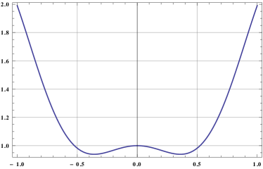
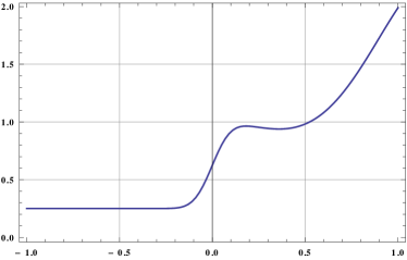
Figure 1: The function $q$ defined by formula (298) in Section 5.1 (left) and the windowed version $\tilde{q}$ of $q$ (right).

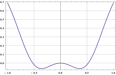
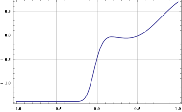
Figure 2: Plots of the solution $r$ of the logarithm form of Kummer’s equation associated with the ordinary differential equation (297) in Section 5.1 when $\lambda=10^{7}$ (left) and the function $r_{1}$ constructed as an intermediate step by the algorithm of Section 4 (right).

Plots of the function $q$ defined by (298) and the windowed version of $q$ constructed as an intermediate step by the algorithm of Section 4 are shown in Figure 1. Plots of the solution $r$ of the logarithm form of Kummer’s equation when $\lambda=10^{7}$ and the windowed version $r_{1}$ of $r$ constructed as an intermediate step by the algorithm of Section 4 are shown in Figure 2.

5.2 Phase functions for Chebyshev’s equation

Chebyshev’s equation

$$(1-t^{2})y^{\prime\prime}(t)-ty^{\prime}(t)+\lambda^{2}y(t)=0\ \ \ \mbox{for all}\ \ -1\leq t\leq 1$$ (299)

admits an exact nonoscillatory phase function which can be represented via elementary functions. More specifically,

$$\alpha_{0}(t)=\lambda\arccos(t)$$ (300)

is a nonoscillatory phase function for the second order equation

$$\psi^{\prime\prime}(t)+\left(\frac{2+t^{2}+4\lambda^{2}\left(1-t^{2}\right)}{4\left(1-t^{2}\right)^{2}}\right)\psi(t)=0\ \ \ \mbox{for all}\ \ \ -1\leq t\leq 1$$ (301)

obtained by introducing

$$\psi(t)=(1-t^{2})^{1/4}y(t)$$ (302)

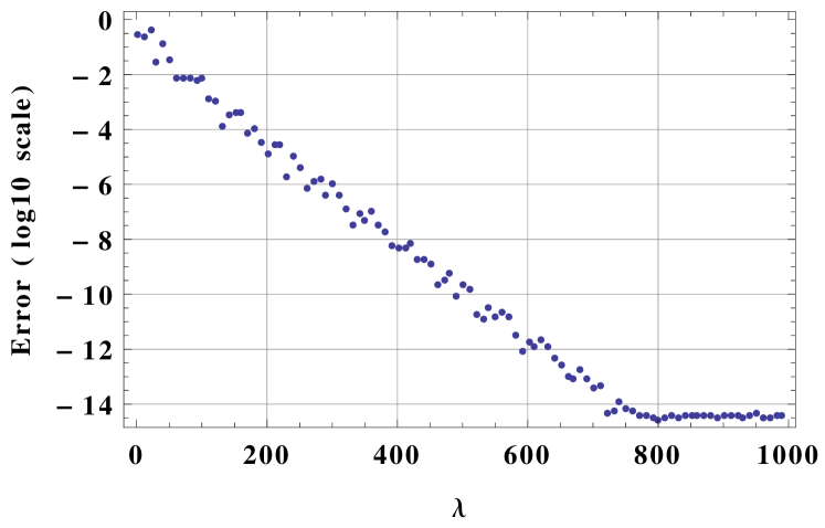
Figure 3: A plot of the base-$10$ logarithm of the relative difference between phase function obtained by applying the algorithm of this paper to Chebyshev’s equation (301) and the well-known nonoscillatory phase function $\lambda\arccos(t)$ for Chebyshev’s equation.

into (299). For each $\lambda=10,20,\ldots,1000$, we applied the algorithm of Section 4 to (301) and compared the resulting phase function to (300). Figure 3 displays a plot of the relative difference

$$\frac{\left\|\alpha-\alpha_{0}\right\|_{\infty}}{\left\|\alpha_{0}\right\|_{\infty}}$$ (303)

between the exact phase function $\alpha_{0}$ and the phase function $\alpha$ obtained via the algorithm of Section 4 as a function of $\lambda$. We observe that as $\lambda$ increases, the difference between the phase function obtained via the algorithm and the function $\lambda\arccos(t)$ decays at an exponential rate.

5.3 Evaluation of Bessel functions.

We compared the cost of evaluating Bessel functions of integer order via the standard recurrence relation with that of doing so using a nonoscillatory phase function.

We denote by $J_{\nu}$ the Bessel function of the first kind of order $\nu$. It is a solution of the second order differential equation

$$t^{2}y^{\prime\prime}(t)+ty^{\prime}(t)+(t^{2}-\nu^{2})y(t)=0,$$ (304)

which is brought into the standard form

$$\psi^{\prime\prime}(t)+\left(1-\frac{\lambda^{2}-1/4}{t^{2}}\right)\psi(t)=0$$ (305)

via the transformation

$$\psi(t)=\sqrt{t}\ y(t).$$ (306)

An inspection of (305) reveals that $J_{\nu}$ is nonoscillatory on the interval

$$\left(0,\frac{1}{2}\sqrt{4\nu^{2}-1}\right)$$ (307)

and oscillatory on the interval

$$\left(\frac{1}{2}\sqrt{4\nu^{2}-1},\infty\right).$$ (308)

In addition to being a solution of a second order differential equation, the Bessel function of the first kind of order $\nu$ satisfies the three-term recurrence relation

$$J_{\nu+1}(t)=\frac{2\nu}{t}J_{\nu}(t)-J_{\nu-1}(t).$$ (309)

The recurrence (309) is numerically unstable in the forward direction; however, when evaluated in the direction of decreasing index, it yields a stable mechanism for evaluating Bessel functions of integer order (see, for instance, Chapter 3 of [20]). These and many other properties of Bessel functions are discussed in [26].

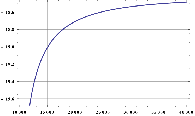
Figure 4: A plot of the nonoscillatory phase function for Bessel’s equation (304) when $n=10^{4}$.

For each of $8$ values of $n$, we obtained an approximation of the Bessel function $J_{n}$ via the algorithm of Section 4 and compared its values to those obtained through the recurrence relation at a collection of $1000$ randomly chosen points in the interval $[\frac{1}{2}\sqrt{4n^{2}-1},10n]$. The results of this experiment are shown in Table 2. The phase function produced by the algorithm of Section 4 when $n=10^{4}$ is shown in Figure 4.

5.4 Evaluation of Legendre functions

We used the algorithm of this paper to evaluate Legendre functions of the first kind of various orders on the interval $[-1,1]$.

For each real number $\nu$, we denote by $P_{\nu}$ the Legendre function of the first kind of order $\nu$. It is the solution of Legendre’s equation

$$(1-t^{2})y^{\prime\prime}(t)-2ty^{\prime}(t)+\nu(\nu+1)y(t)=0\ \ \ \mbox{for all}\ \ -1\leq t\leq 1$$ (310)

which is regular at the origin. Letting

$$\psi(t)=\sqrt{1-t^{2}}\ y(t)$$ (311)

in Equation (310) yields

$$\psi^{\prime\prime}(t)+\left(\frac{1}{(1-t^{2})^{2}}+\frac{\nu}{1-t^{2}}+\frac{\nu^{2}}{(1-t^{2})^{2}}\right)\psi(t)=0\ \ \ \mbox{for all}\ \ -1\leq t\leq 1,$$ (312)

which is in a suitable form for the algorithm of Section 4.

We observe that the coefficient in equation (312) is singular at $\pm 1$, which means that phase functions for Legendre’s equation are singular at $\pm 1$ as well. Accordingly, in this experiment we used as input to the algorithm of Section 4 a partition of the form

$$-\xi_{-k}<-\xi_{-k+1}<\ldots<\xi_{-1}<\xi_{0}<\xi_{1}<\ldots\xi_{k-1}<\xi_{k},$$ (313)

where $k=50$ and $\xi_{j}$ is defined by the formula

$$\xi_{j}=1-2^{-|j|}.$$ (314)

The set $\{\xi_{j}\}$ is a “graded mesh” whose points cluster near the singularities $\pm 1$ of the coefficient in (312). Note that (313) is not a partition of the entire interval $[-1,1]$ but rather a partition of $[-b,b]$, where

$$b=1-2^{-50}.$$ (315)

Functions were represented using $16^{th}$ order Chebyshev expansions on each of the intervals $[\xi_{j},\xi_{j+1}]$.

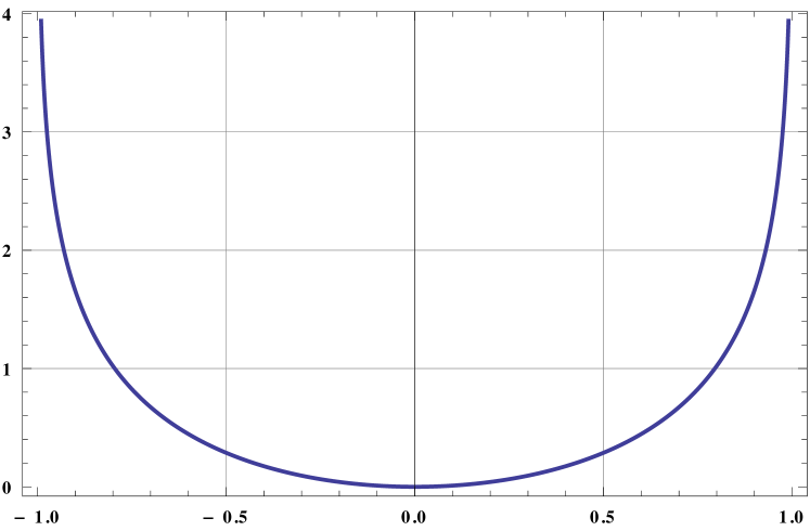
Figure 5: A plot of the nonoscillatory solution of the logarithm form of Kummer’s equation associated with Legendre’s differential equation (310) when $\nu=\pi 10^{5}$. This function has singularities at the points $\pm 1$ and is represented using a graded mesh which becomes dense near them.

For each of $11$ values of $\nu$, the algorithm of this paper was applied to Equation (312) and the solution evaluated at a collection of $1000$ randomly chosen points on the interval $[-1,1]$. In order to assess the the error in each obtained solution, we constructed a reference solutions by performing the calculations a second time using extended precision (Fortran REAL*16) arithmetic. The results are reported in Table 3. Each row corresponds to one value of $\nu$ and reports the time required to construct the nonoscillatory phase functions, the average time required to evaluate the Legendre function of the first kind of order $\nu$ using this nonoscillatory phase function, and the maximum observed absolute error. Figure 5 depicts the solution of the logarithm form of Kummer’s equation obtained by the algorithm of this paper when $\nu=\pi\cdot 10^{5}$.

5.5 Evaluation of prolate spheriodal wave functions

We used the algorithm of Section 4 to evaluate prolate spheriodal wave functions of order 0 and we compared its performance with that of the Osipov-Rokhlin algorithm [21].

Suppose that $c>0$ is a real number. Then there exists a sequence

$$0<\chi_{c,0}<\chi_{c,1}<\chi_{c,2}<\cdots$$ (316)

of positive real numbers such for each nonnegative integer $n$, the second order differential equation

$$(1-t^{2})\psi^{\prime\prime}(t)-2t\psi^{\prime}(t)+(\chi_{c,n}-c^{2}t^{2})\psi(t)=0$$ (317)

has a continuous solution on the interval $[-1,1]$. These solutions are the prolate spheriodial wave functions of order $0$ associated with the parameter $c$. We denote them by

$$\psi_{c,0}(t),\psi_{c,1}(t),\psi_{c,2}(t),\ldots.$$ (318)

The monograph [22] contains a detailed discussion of the prolate spheriodal wave functions of order $0$.

By introducing the function

$$\varphi(t)=\psi(t)\sqrt{1-t^{2}}$$ (319)

into (317), we bring it into the form

$$\varphi^{\prime\prime}(t)+\left(\frac{1}{(1-t^{2})^{2}}+\frac{\chi_{c,n}}{1-t^{2}}-c^{2}t^{2}\right)\varphi(t)=0.$$ (320)

An inspection of (320) reveals that the coefficient in (320) is nonnegative on the interval $[-1,1]$ when $\chi_{n}\geq c^{2}$.

For several values of $c$ and $\chi_{n,c}>c^{2}$, we evaluated the prolate spheriodial wave function $\psi_{c,n}$ at a collection of $100$ randomly chosen points in the interval $[-1,1]$ by applying the algorithm of Section 4 to (320) and via the Osipov-Rokhlin algorithm. Table 4 presents the results and Figure 6 shows a plot of $\alpha(t)-ct$, where $c=10^{5}$, $n=63769$, $\chi_{c,n}=1.00060408908491\times 10^{10}$ and $\alpha$ is the nonoscillatory phase function for Equation (320) produced by the algorithm of Section 4.

6 Acknowledgments

The author would like to thank Vladimir Rokhlin for reading a draft of this manuscript and for his many helpful suggestions, and Andrei Osipov for providing his code for evaluating prolate spheriodal wave functions. James Bremer was supported by a fellowship from the Alfred P. Sloan Foundation, and by National Science Foundation grant DMS-1418723.

7 References

$\lambda$	Phase function	Avg. phase function	Maximum
	construction time	evaluation time	error
$10^{1}$	$7.25\times 10^{-02}$	$1.55\times 10^{-06}$	$6.93\times 10^{-14}$
$10^{2}$	$9.17\times 10^{-02}$	$1.58\times 10^{-06}$	$5.39\times 10^{-13}$
$10^{3}$	$6.74\times 10^{-02}$	$1.55\times 10^{-06}$	$3.01\times 10^{-12}$
$10^{4}$	$6.73\times 10^{-02}$	$1.55\times 10^{-06}$	$4.82\times 10^{-11}$
$10^{5}$	$6.72\times 10^{-02}$	$1.59\times 10^{-06}$	$3.23\times 10^{-10}$
$10^{6}$	$6.66\times 10^{-02}$	$1.64\times 10^{-06}$	$5.15\times 10^{-09}$
$10^{7}$	$8.60\times 10^{-02}$	$1.61\times 10^{-06}$	$3.64\times 10^{-08}$

Table 1: The accuracy and running time of the algorithm of this paper when applied to to the initial value problem (297) of Section 5.1.

$n$	Phase function	Avg. phase function	Avg. recurrence	Maximum
	construction time	evaluation time	evaluation time	error
$10^{1}$	1.70$\times 10^{-02}$ secs	2.24$\times 10^{-07}$ secs	1.40$\times 10^{-06}$ secs	1.58$\times 10^{-14}$
$10^{2}$	2.27$\times 10^{-02}$ secs	2.06$\times 10^{-07}$ secs	6.17$\times 10^{-06}$ secs	1.75$\times 10^{-14}$
$10^{3}$	1.62$\times 10^{-02}$ secs	2.23$\times 10^{-07}$ secs	4.60$\times 10^{-05}$ secs	4.62$\times 10^{-14}$
$10^{4}$	1.65$\times 10^{-02}$ secs	2.24$\times 10^{-07}$ secs	4.29$\times 10^{-04}$ secs	3.52$\times 10^{-13}$
$10^{5}$	1.62$\times 10^{-02}$ secs	2.29$\times 10^{-07}$ secs	4.12$\times 10^{-03}$ secs	4.70$\times 10^{-13}$
$10^{6}$	1.66$\times 10^{-02}$ secs	2.65$\times 10^{-07}$ secs	4.20$\times 10^{-02}$ secs	1.66$\times 10^{-12}$
$10^{7}$	2.94$\times 10^{-02}$ secs	2.69$\times 10^{-07}$ secs	4.22$\times 10^{-01}$ secs	3.88$\times 10^{-11}$
$10^{8}$	6.42$\times 10^{-01}$ secs	6.39$\times 10^{-07}$ secs	4.33$\times 10^{+00}$ secs	3.91$\times 10^{-11}$

Table 2: A comparison of the time required to evaluate the Bessel function $J_{n}$ using the standard recurrence relation with that required to evaluate it using a nonoscillatory phase function. The recurrence relation approach scales as $O(n)$ in the order $n$ while the time required by the phase function method is $O(1)$.

$\nu$	Phase function	Avg. phase function	Maximum
	construction time	evaluation time	error
$\pi\cdot 10^{4}$	2.92$\times 10^{-03}$ secs	3.13$\times 10^{-07}$ secs	1.32$\times 10^{-13}$
$\pi\cdot 10^{5}$	2.60$\times 10^{-03}$ secs	3.84$\times 10^{-07}$ secs	3.24$\times 10^{-13}$
$\pi\cdot 10^{6}$	2.46$\times 10^{-03}$ secs	4.63$\times 10^{-07}$ secs	1.09$\times 10^{-12}$
$\pi\cdot 10^{7}$	2.97$\times 10^{-03}$ secs	3.67$\times 10^{-07}$ secs	3.21$\times 10^{-12}$
$\pi\cdot 10^{8}$	2.53$\times 10^{-03}$ secs	3.61$\times 10^{-07}$ secs	1.35$\times 10^{-11}$
$\sqrt{2}\cdot 10^{4}$	5.61$\times 10^{-03}$ secs	3.20$\times 10^{-07}$ secs	7.22$\times 10^{-13}$
$\sqrt{2}\cdot 10^{5}$	5.43$\times 10^{-03}$ secs	3.54$\times 10^{-07}$ secs	3.32$\times 10^{-12}$
$\sqrt{2}\cdot 10^{6}$	2.49$\times 10^{-03}$ secs	4.26$\times 10^{-07}$ secs	1.13$\times 10^{-12}$
$\sqrt{2}\cdot 10^{7}$	2.61$\times 10^{-03}$ secs	3.84$\times 10^{-07}$ secs	2.79$\times 10^{-12}$
$\sqrt{2}\cdot 10^{8}$	5.43$\times 10^{-03}$ secs	3.67$\times 10^{-07}$ secs	8.65$\times 10^{-12}$
$\sqrt{2}\cdot 10^{9}$	4.94$\times 10^{-03}$ secs	3.95$\times 10^{-07}$ secs	2.85$\times 10^{-11}$

Table 3: The results obtained by applying the algorithm of Section 4 to Legendre’s differential equation (310). We observe that the running time is independent of $\nu$, but that some accuracy is lost when evaluating Legendre functions of large orders.

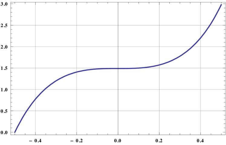
Figure 6: A plot of the function $\alpha(t)-ct$, where $\alpha$ is nonoscillatory phase function associated with equation (320), $c=10^{5}$, $n=63769$ , and $\chi_{n,c}=1.00060408908491\times 10^{10}$.

$c$	$n$	$\chi_{c,n}$		Avg. phase	Average
			Phase function	function	Osipov-Rokhlin	Maximum
			construction time	evaluation time	evaluation time	error
$10^{4}$	$12904$	$2.18416195669669\times 10^{+08}$	3.30$\times 10^{-02}$ secs	3.22$\times 10^{-07}$ secs	1.65$\times 10^{-04}$ secs	3.24$\times 10^{-11}$
$10^{5}$	$63769$	$1.00060408908491\times 10^{+10}$	3.29$\times 10^{-02}$ secs	3.29$\times 10^{-07}$ secs	1.11$\times 10^{-03}$ secs	1.67$\times 10^{-10}$
$10^{5}$	$95653$	$1.44996988449419\times 10^{+10}$	3.32$\times 10^{-02}$ secs	3.19$\times 10^{-07}$ secs	1.34$\times 10^{-03}$ secs	2.00$\times 10^{-10}$
$10^{6}$	$636748$	$1.00005993679849\times 10^{+12}$	3.31$\times 10^{-02}$ secs	3.70$\times 10^{-07}$ secs	1.14$\times 10^{-02}$ secs	1.77$\times 10^{-09}$
$10^{6}$	$1910244$	$4.15761057502686\times 10^{+12}$	3.30$\times 10^{-02}$ secs	3.60$\times 10^{-07}$ secs	2.34$\times 10^{-02}$ secs	5.19$\times 10^{-09}$
$10^{7}$	$12732696$	$2.14063766093698\times 10^{+14}$	3.08$\times 10^{-02}$ secs	3.60$\times 10^{-07}$ secs	1.59$\times 10^{-01}$ secs	3.74$\times 10^{-08}$
$10^{8}$	$127324798$	$2.14057058422053\times 10^{+16}$	4.34$\times 10^{-02}$ secs	4.10$\times 10^{-07}$ secs	1.59$\times 10^{+00}$ secs	3.30$\times 10^{-07}$
$10^{8}$	$190986447$	$4.15616226165926\times 10^{+16}$	4.32$\times 10^{-02}$ secs	3.60$\times 10^{-07}$ secs	2.22$\times 10^{+00}$ secs	4.35$\times 10^{-07}$
$10^{9}$	$636619965$	$1.00000005945416\times 10^{+18}$	4.31$\times 10^{-02}$ secs	4.01$\times 10^{-07}$ secs	1.15$\times 10^{+01}$ secs	8.61$\times 10^{-07}$

Table 4: A comparison of the results obtained by using the algorithm of this paper to evaluate prolate spheriodial wave functions of order $0$ with those obtained via the Osipov-Rokhlin algorithm [21].

References

- [1] Andrews, G., Askey, R., and Roy, R. Special Functions. Cambridge University Press, 1999.
- [2] Bellman, R. Stability Theory of Differential Equations. Dover Publications, 1953.
- [3] Bogaert, I., Michiels, B., and Fostier, J. computation of Legendre polynomials and Gauss-Legendre nodes and weights for parallel computing. SIAM Journal on Scientific Computing 34 (2012), C83–C101.
- [4] Borůvka, O. Linear Differential Transformations of the Second Order. The English University Press, 1971.
- [5] Bremer, J., and Rokhlin, V. Improved estimates for nonoscillatory phase functions. arXiv:1505.05548 (2015).
- [6] Coddington, E., and Levinson, N. Theory of Ordinary Differential Equations. Krieger Publishing Company, 1984.
- [7] Corless, R., Gonnet, G., Hare, D., Jeffrey, D., and Knuth, D. On the Lambert function. Advances in Computational Mathematics 5 (1996), 329–359.
- [8] Daalhuis, A. O. Hyperasymptotic solutions of second-order linear differential equations. II. Methods and Applications of Analysis 2 (1995), 198–211.
- [9] Daalhuis, A. O., and Olver, F. W. J. Hyperasymptotic solutions of second-order linear differential equations. I. Methods and Applications of Analysis 2 (1995), 173–197.
- [10] Dutt, A., Greengard, L., and Rokhlin, V. Spectral deferred correction methods for ordinary differential equations. BIT Numerical Mathematics 40 (2000), 241–266.
- [11] Goldstein, M., and Thaler, R. M. Bessel functions for large arguments. Mathematical Tables and Other Aids to Computation 12 (1958), 18–26.
- [12] Grafakos, L. Classical Fourier Analysis. Springer, 2009.
- [13] Grafakos, L. Modern Fourier Analysis. Springer, 2009.
- [14] Heitman, Z., Bremer, J., and Rokhlin, V. On the existence of nonoscillatory phase functions for second order ordinary differential equations in the high-frequency regime. Journal of Computational Physics 290 (2015), 1–27.
- [15] Heitman, Z., Bremer, J., Rokhlin, V., and Vioreanu, B. On the asymptotics of Bessel functions in the Fresnel regime. Applied and Computational Harmonic Analysis (to appear).
- [16] Hörmader, L. The Analysis of Linear Partial Differential Operators I, second ed. Springer, 1990.
- [17] Hörmader, L. The Analysis of Linear Partial Differential Operators II, second ed. Springer, 1990.
- [18] Kummer, E. De generali quadam aequatione differentiali tertti ordinis. Progr. Evang. Köngil. Stadtgymnasium Liegnitz (1834).
- [19] Neuman, F. Global Properties of Linear Ordinary Differential Equations. Kluwer Academic Publishers, 1991.
- [20] Olver, F., Lozier, D., Boisvert, R., and Clark, C. NIST Handbook of Mathematical Functions. Cambridge University Press, 2010.
- [21] Osipov, A., and Rokhlin, V. On the evaluation of prolate spheroidal wave functions and associated quadrature rules. Applied and Computational Harmonic Analysis 36 (2014), 108–142.
- [22] Osipov, A., Rokhlin, V., and Xiao, H. Prolate Spheriodal Wave Functions of Order . Springer, 2013.
- [23] Spigler, R., and Vianello, M. The phase function method to solve second-order asymptotically polynomial differential equations. Numerische Mathematik 121 (2012), 565–586.
- [24] Szegö, G. Orthogonal Polynomials. American Mathematical Society, 1959.
- [25] Trefethen, N. Approximation Theory and Approximation Practice. Society for Industrial and Applied Mathematics, 2013.
- [26] Watson, G. N. A Treatise on the Theory of Bessel Functions, second ed. Cambridge University Press, 1995.