The production and decay of the top partner $T$ in the left-right twin higgs model at the ILC and CLIC

Abstract

The left-right twin Higgs model (LRTHM) predicts the existence of the top partner $T$. In this work, we make a systematic investigation for the single and pair production of this top partner $T$ through the processes: $e^{+}e^{-}\to t\overline{T}+T\bar{t}$ and $T\overline{T}$, the neutral scalar (the SM-like Higgs boson $h$ or neutral pseudoscalar boson $\phi^{0}$) associate productions $e^{+}e^{-}\to t\overline{T}h+T\bar{t}h$, $T\overline{T}h$, $t\overline{T}\phi^{0}+T\bar{t}\phi^{0}$ and $T\overline{T}\phi^{0}$. From the numerical evaluations for the production cross sections and relevant phenomenological analysis we find that (a) the production rates of these processes, in the reasonable parameter space, can reach the level of several or tens of fb; (b) for some cases, the peak value of the resonance production cross section can be enhanced significantly and reaches to the level of pb; (c) the subsequent decay of $T\to\phi^{+}b\to t\bar{b}b$ may generate typical phenomenological features rather different from the signals from other new physics models beyond the standard model(SM); and (d) since the relevant SM background is generally not large, some signals of the top partner $T$ predicted by the LRTHM may be detectable in the future ILC and CLIC experiments.

I Introduction

With the observation of a standard model (SM) Higgs boson with a mass around 125 GeV atlas ; cms ; lhcphysics at the Large Hadron Collider (LHC), our understanding of electroweak symmetry breaking (EWSB) has been significantly improved than before lhcphysics . However, this does not necessarily mean that the SM is fundamentally the whole story zhu . It is well known that the SM has a serious problem called the little hierarchy problem 0007265 . The twin Higgs mechanism twin1 ; twin2 has been proposed recently to tackle this little hierarchy problem, in which the SM-like Higgs emerges as a pseudo-Goldstone boson once a global symmetry is spontaneously broken. The twin Higgs theories use a discrete symmetry in combination with an approximate global symmetry to eliminate one-loop quadratic divergence and thus stabilizing the mass of Higgs boson.

The twin Higgs mechanism can be implemented in left-right models with the additional discrete symmetry being identified with left-right symmetry ly . The left-right twin Higgs model (LRTHM) is a concrete realization of the twin Higgs mechanism Hock . In this model, the SM gauge symmetry is extended to $SU(2)_{L}\times SU(2)_{R}\times U(1)_{B-L}$, which is embedded into the global $U(4)_{1}\times U(4)_{2}$ symmetry. The leading quadratically divergent contributions of the SM gauge bosons to the Higgs boson mass are canceled by the loop involving the new heavy gauge bosons ($W^{\pm}_{H},Z_{H}$), while those for the top quark can be canceled by the contributions from a heavy top partner ($T$). These new particles predicted by the LRTHM at or below the TeV scale, which might generate characteristic signatures at the present and future high energy colliders Hock ; twin2 ; dong ; lei ; liu ; ycx . Very recently, we have studied the properties of the LRTHM confronted with the latest LHC Higgs data liuprd .

Recently, many searches have been performed by both ATLAS atlas-1 ; atlas-2 and CMS cms-1 ; cms-2 collaborations in order to discover or set bounds on the heavy top-quark partner, assuming decays into three channels, $W^{+}b$, $Zt$ and $ht$, and scanning over various combinations of the branching ratios. For instance, top partner with masse below $656$ GeV are excluded at $95\%$ confidence level under the assumption of a branching ratio $BR(T\rightarrow W^{+}b)=1$ atlas-3 . However, the dominant decay mode for the top partner in the LRTHM is into a charged Higgs boson and a bottom quark. Thus, the current bound on the top partner will be relaxed. The production of the $T$-quark at the LHC have been described in Ref. Hock , in which the $s$-channel on shell $W_{H}$ decay dominated the single heavy top production. The single production of the top partner via the $e\gamma$ and $\gamma\gamma$ fusion processes has been studied in Refs. st1 ; st2 .

So far, most of the works about the top partner focus on phenomenological analysis at the LHC experiments, see for example Refs. t-lhc1 ; t-lhc2 ; t-lhc3 . When compared with the LHC, a TeV scale linear $e^{+}e^{-}$ collider has a particularly clear background environment, with a center of mass(c.m.) energy in the range of 500 to 1600 GeV, as in the case of the International Linear Collider(ILC) ILC , and of 3 TeV to the Compact Linear Collider(CLIC) CLIC . The high luminosity linear collider is thus a precision machine with which the properties of new particles can be measured precisely. For example, the final stage of CLIC operating at an energy of 3 TeV is expected to directly examine the pair production of new heavy top partner of mass up to 1.5 TeV CLIC1 . A detailed study of the anomalous single fourth generation $t^{\prime}$ quark production at ILC and CLIC has been performed in ref. npb-851-289 . The phenomenology of top partners in the little Higgs models with T-parity (LHT) and the minimal supersymmetric standard model with R-parity (MSSMR) at future linear colliders are studied in Refs. t-ilc1 ; t-ilc2 , in which the decay signal of $T$-quark ($T\to tA_{H}$) can fake the signal of the scalar top quark $\tilde{t}\rightarrow t\tilde{\chi}_{0}^{1}$. In the LRTHM, furthermore, the dominant decay mode $T\rightarrow\phi^{+}b\rightarrow t\bar{b}b$ may generate different phenomenological features. Thus, in this paper, we will perform a comprehensive analysis on six top partner production processes: $e^{+}e^{-}\rightarrow t\overline{T}+T\bar{t},T\overline{T},t\overline{T}h+T\bar{t}h,T\overline{T}h,t\overline{T}\phi^{0}+T\bar{t}\phi^{0}$ and $e^{+}e^{-}\rightarrow T\overline{T}\phi^{0}$ at the future possible ILC and/or CLIC experiments.

This paper is organized as follows. In section II, we give a brief review of the LRTHM, and then study the decays of the top partner and the charged Higgs bosons. Sec. III is devoted to the computation of the production cross section (CS) of above mentioned six production channels. Some phenomenological analysis are also included in these three sections. Our conclusions are given in section IV.

II Overview of the LRTHM

The details of the LRTHM and some phenomenology analysis have been studied in Ref. Hock . Thus we will focus on the top partner sector in this section. In the LRTHM, two Higgs fields ($H$ and $\hat{H}$) are introduced and each transforms as $(4,1)$ and $(1,4)$ respectively under the global symmetry. They are written as

$$H=\left(\begin{array}[]{c}H_{L}\\ H_{R}\\ \end{array}\right)\,,~{}~{}~{}~{}~{}~{}~{}~{}~{}~{}~{}~{}~{}~{}\hat{H}=\left(\begin{array}[]{c}\hat{H}_{L}\\ \hat{H}_{R}\\ \end{array}\right)\,,$$ (5)

where $H_{L,R}$ and $\hat{H}_{L,R}$ are two component objects which are charged under the $SU(2)_{L}\times SU(2)_{R}\times U(1)_{B-L}$ as

$$H_{L}~{}and~{}\hat{H}_{L}:(2,1,1),~{}~{}~{}~{}~{}~{}~{}~{}H_{R}~{}and~{}\hat{H}_{R}:(1,2,1).$$ (6)

The global $U(4)_{1}(U(4)_{2})$ symmetry is spontaneously broken down to its subgroup $U(3)_{1}(U(3)_{2})$ with non-zero vacuum expectation values (VEV) as $\langle H\rangle=(0,0,0,f)$ and $\langle\hat{H}\rangle=(0,0,0,\hat{f})$. Each spontaneously symmetry breaking yields seven Nambu-Goldstone bosons. The gauge symmetry $SU(2)_{L}\times SU(2)_{R}\times U(1)_{B-L}$ is eventually broken down to the SM $U(1)_{em}$, six out of the 14 Goldstone bosons are eaten by the SM gauge bosons $(W^{\pm},Z)$ and the heavy gauge bosons $(W_{H}^{\pm},Z_{H})$ in the LRTH model. After the re-parametrization of the fields, the remaining 8 particles include one SM-like Higgs boson $h$, one neutral pseudoscalar $\phi^{0}$, a pair of charged scalar $\phi^{\pm}$ and an extra $SU(2)_{L}$ doublet $\hat{h}=(\hat{h}_{1}^{+},\hat{h}_{2}^{0})$. The lightest particle in the odd $\hat{h}_{2}^{0}$ is stable, and thus can be a candidate for dark matter.

The masses of the heavy gauge bosons are expressed as:

$$M_{W_{H}}^{2} = \frac{1}{2}g^{2}(\hat{f}^{2}+f^{2}\cos^{2}x),$$ (7)

$$M_{Z_{H}}^{2} = \frac{g^{2}+g^{\prime 2}}{g^{2}}(M_{W}^{2}+M_{W_{H}}^{2})-M_{Z}^{2},$$ (8)

where $x=v/(\sqrt{2}f)$ and $v$ is the electroweak scale, the values of $f$ and $\hat{f}$ are interconnected once we set $v=246$ GeV. The Weinberg angle can be written as:

$$s_{W}=\sin\theta_{W}=\frac{g^{\prime}}{\sqrt{g^{2}+2g^{\prime 2}}},~{}~{}~{}~{}~{}~{}~{}~{}c_{W}=\cos\theta_{W}=\sqrt{\frac{g^{2}+g^{\prime 2}}{g^{2}+2g^{\prime 2}}}.$$ (9)

Besides the SM-like Higgs boson $h$, both the charged scalars $\phi^{\pm}$ and the neutral pseudoscalar $\phi^{0}$ can couple to both the fermions and the gauge bosons. Their masses can be obtained from the one-loop Coleman-Weinberg (CW) potential and the soft left-right symmetry breaking terms, so-called $\mu-$term Hock :

$$V_{\mu}=-\mu_{r}^{2}(H_{R}^{\dagger}\hat{H}_{R}+h.c.)+\hat{\mu}^{2}H_{L}^{\dagger}\hat{H}_{L}.$$ (10)

Here $\hat{\mu}$ is of the order of $f$ or smaller, and $\mu_{r}$ should be less than about $f/4\pi$ in order not to reintroduce fine tuning Hock . The masses of $\phi^{0}$ and $\phi^{\pm}$ can therefore be written as the form of

$$m^{2}_{\phi^{0}} = \frac{\mu_{r}^{2}f\hat{f}}{\hat{f}^{2}+f^{2}\cos^{2}x}\cdot\left\{\frac{\hat{f}^{2}\left[\cos x+\frac{\sin x}{x}(3+x^{2})\right]}{f^{2}\left(\cos x+\frac{\sin x}{x}\right)^{2}}+2\cos x+\frac{f^{2}\cos^{2}x(1+\cos x)}{2\hat{f}^{2}}\right\},$$ (11)

$$m^{2}_{\phi^{\pm}} = \frac{3}{16\pi^{2}}\frac{g^{\prime 2}M^{2}_{W_{H}}}{M^{2}_{Z_{H}}-M^{2}_{Z}}\Big{[}(\frac{M^{2}_{W}}{M^{2}_{Z_{H}}}-1){\mathcal{Z}}(M_{Z_{H}})-(\frac{M^{2}_{W}}{M^{2}_{Z}}-1){\mathcal{Z}}(M_{Z})\Big{]}$$ (12)

$$\,+\frac{\mu_{r}^{2}f\hat{f}}{\hat{f}^{2}+f^{2}\cos^{2}x}(\frac{\hat{f}^{2}x}{f^{2}\sin x}+2\cos x+\frac{f^{2}\cos^{3}x}{\hat{f}^{2}}),$$

where ${\mathcal{Z}}(x)=-x^{2}(\ln\frac{\Lambda^{2}}{x^{2}}+1)$, and the cut-off scale $\Lambda$ is typically taken to be $4\pi f$. In the allowed parameters space, the masses of the charged scalars $\phi^{\pm}$ are generally in the range of a few hundred GeV. The value of $m_{\phi^{0}}^{2}$ depend on two parameters $\mu_{r}$ and $f$, and the lower limit comes from the non-observation of the decay $\Upsilon\to\gamma+X_{0}$ cons-phi0 .

II.1 Masses and relevant couplings of top quark sector

In order to cancel the one-loop quadratic divergence of Higgs mass induced by top quark, a pair of vector-like quarks ($U_{L},U_{R}$) are introduced, which are singlets under $SU(2)_{L}\times SU(2)_{R}$. The Lagrangian can be written as Hock

$${\cal L}_{t}=y_{L}\bar{Q}_{L3}\tau_{2}H_{L}^{*}U_{R}+y_{R}\bar{Q}_{R3}\tau_{2}H_{R}^{*}U_{L}-M\bar{U}_{L}U_{R}+h.c.$$ (13)

where $Q_{L3}=-i(u_{L3},d_{L3})^{T}$ and $Q_{R3}=(u_{R3},d_{R3})^{T}$. Under left-right symmetry, $y_{L}=y_{R}=y$. The mass eigenstates for the top quark $t$ and heavy top partner $T$ can be obtained by diagonalizing the mass matrix. Their masses and relevant couplings to gauge bosons are given by Hock

$$m_{t}^{2} = \frac{1}{2}(M^{2}+y^{2}f^{2}-N_{t}),~{}~{}~{}~{}~{}~{}~{}~{}m_{T}^{2}=\frac{1}{2}(M^{2}+y^{2}f^{2}+N_{t}),$$ (14)

$$Z_{\mu}t\bar{T} : e\gamma_{\mu}(C_{L}S_{L}\hat{f}^{2}c^{2}_{W}P_{L}+f^{2}x^{2}s^{2}_{W}C_{R}S_{R}P_{R}/(2\hat{f}^{2}c^{3}_{W});$$ (15)

$$Z_{H\mu}t\bar{T} : e\gamma_{\mu}(C_{L}S_{L}s^{2}_{W}P_{L}-c^{2}_{W}C_{R}S_{R}P_{R}/(2s_{W}c_{W}c2_{W});$$ (16)

$$Z_{\mu}T\bar{T} : -e\gamma_{\mu}(4s^{2}_{W}-3S^{2}_{L}P_{L})/(6s_{W}c_{W});$$ (17)

$$Z_{H\mu}T\bar{T} : -e\gamma_{\mu}[(3C^{2}_{L}+1)s^{2}_{W}P_{L}-(3c^{2}_{W}C^{2}_{R}-4s^{2}_{W})P_{R}]/(6s_{W}c_{W}c2_{W});$$ (18)

$$Z_{H\mu}t\bar{t} : -e\gamma_{\mu}[(3S^{2}_{L}+1)s^{2}_{W}P_{L}-(3c^{2}_{W}S^{2}_{R}-4s^{2}_{W})P_{R}]/(6s_{W}c_{W}c2_{W}),$$ (19)

where

$$S_{L} = \frac{1}{\sqrt{2}}\sqrt{1-(y^{2}f^{2}\cos 2x+M^{2})/N_{t}},~{}~{}C_{L}=\sqrt{1-S^{2}_{L}},$$ (20)

$$S_{R} = \frac{1}{\sqrt{2}}\sqrt{1-(y^{2}f^{2}\cos 2x-M^{2})/N_{t}},~{}~{}C_{R}=\sqrt{1-S^{2}_{R}},$$ (21)

with $N_{t}=\sqrt{(M^{2}+y^{2}f^{2})^{2}-y^{4}f^{4}\sin^{2}2x}$ and $x=v/(\sqrt{2}f)$.

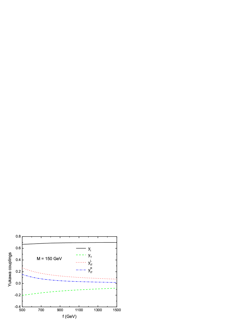
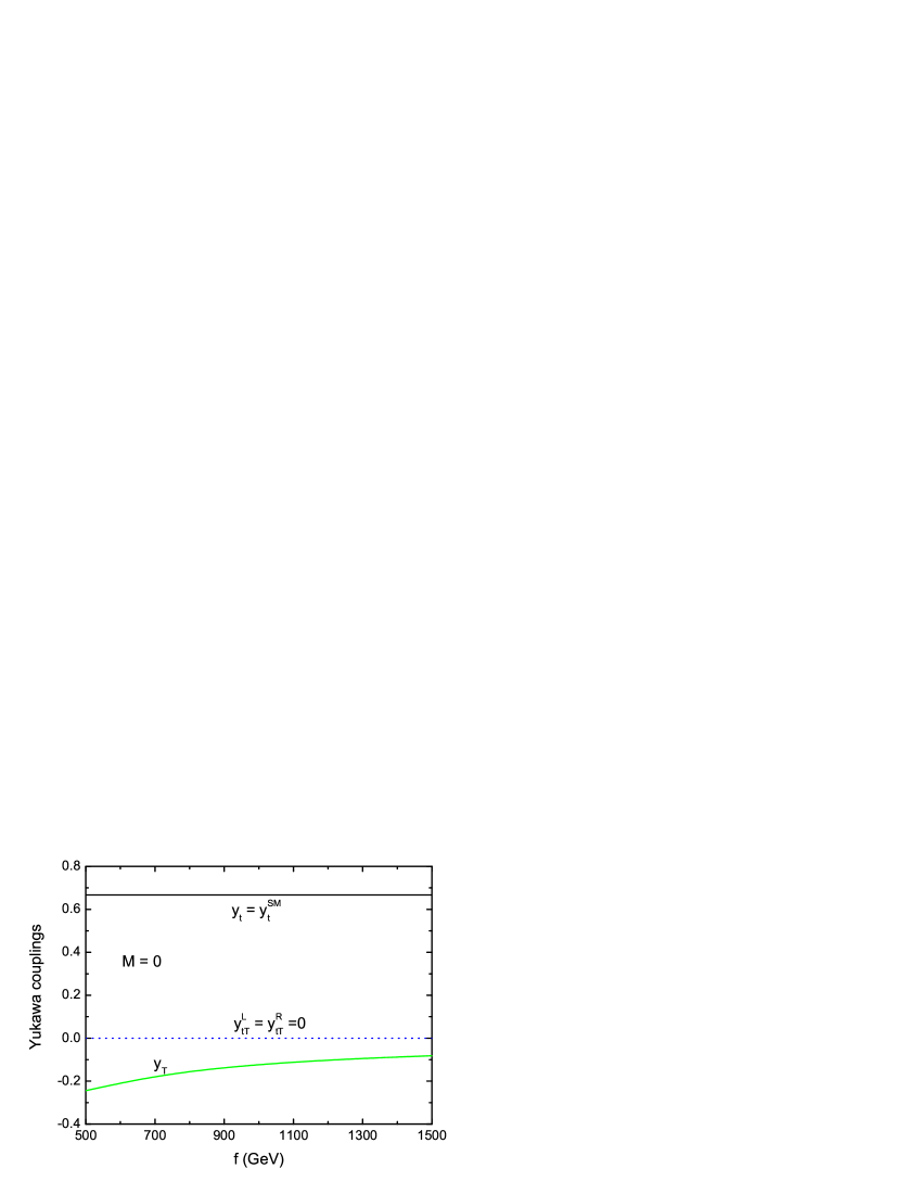
Figure 1: The Yukawa couplings ($y_{t},y_{T},y^{L}_{tT},y^{R}_{tT}$) as a function of the parameter $f$ for two typical values of $M$.

From Eq.(13), we can get the interactions between the Higgs boson and the pairs of $(t\bar{t},T\overline{T},T\bar{t},\overline{T}t)$:

$${\mathcal{L}_{int}}=-y_{t}t\bar{t}h-y_{T}T\bar{T}h-(\bar{T}[y^{L}_{tT}P_{L}+y^{R}_{tT}P_{R}]th+h.c.),$$ (22)

where the Yukawa couplings constants ($y_{t},y_{T},y^{L}_{tT},y^{R}_{tT}$) are defined as

$$y_{t} = -\frac{m_{t}}{v}C_{L}C_{R},~{}~{}~{}~{}~{}~{}~{}~{}~{}~{}~{}~{}~{}~{}~{}~{}~{}~{}~{}~{}~{}y_{T}=-y(S_{R}S_{L}-C_{L}C_{R}x)/\sqrt{2},$$ (23)

$$y^{L}_{tT} = -\frac{y}{\sqrt{2}}(C_{L}S_{R}+S_{L}C_{R}x),~{}~{}~{}~{}~{}~{}y^{R}_{tT}=-\frac{y}{\sqrt{2}}(C_{L}S_{R}x+S_{L}C_{R}).$$ (24)

Since the mixing angles are sensitive to the parameters $M$ and $f$, we plot in Fig. 1 the coupling constants of the Yukawa interactions ($y_{t},y_{T},y^{L}_{tT},y^{R}_{tT}$) as a function of the parameter $f$ for two typical values of $M$: $M=0,150$ GeV. For $M=150$ GeV, the left-handed mixing of top quark and top partner is larger than that for the right-handed ones, while they all equal zero for $M=0$. In this case the top quark is purely $(u_{3L},q_{R})$ and the top partner is purely $(q_{L},u_{3R})$. On the other hand, we can see that the couplings $y_{T}$ and $y_{t}$ have different sign, and $y_{t}$ is almost three times as large as $y_{T}$.

II.2 Decays of the top partner and charged Higgs bosons

In the LRTHM, the top quark partner $T$ can decay into $\phi^{+}b$, $ht$, $Zt$, $Wb$ and $\phi^{0}t$, among which the decay $T\rightarrow\phi^{+}b$ is the most important channel. Here we take the mass of the charged scalars as $m_{\phi^{\pm}}=200$ GeV. In Fig. 2 we show the $M$- and $f$-dependence of the branching ratios of those relevant decays of the top quark partner $T$. As shown in Fig. 2a, more than $60\%$ of top partner decays via $T\rightarrow\phi^{+}b$ for 500 GeV$\leq f\leq$1000 GeV. Other decays are strongly suppressed since the relevant couplings are suppressed by the ratio $(M/f)$. For comparison, the subdominant decay $T\rightarrow Wb$ can have a branching ratio of about $11\%$ for $M=150$ GeV and $f$=500 GeV. This is different from the case of the little Higgs model with T-parity, where the decay $T\rightarrow W^{+}b$ is the dominant channel lht . In the limit $M=0$, the only two body decay mode is $T\rightarrow\phi^{+}b$, with a branching ratio of $100\%$. Thus, the previous bounds on the top partner will be relaxed in the LRTHM.

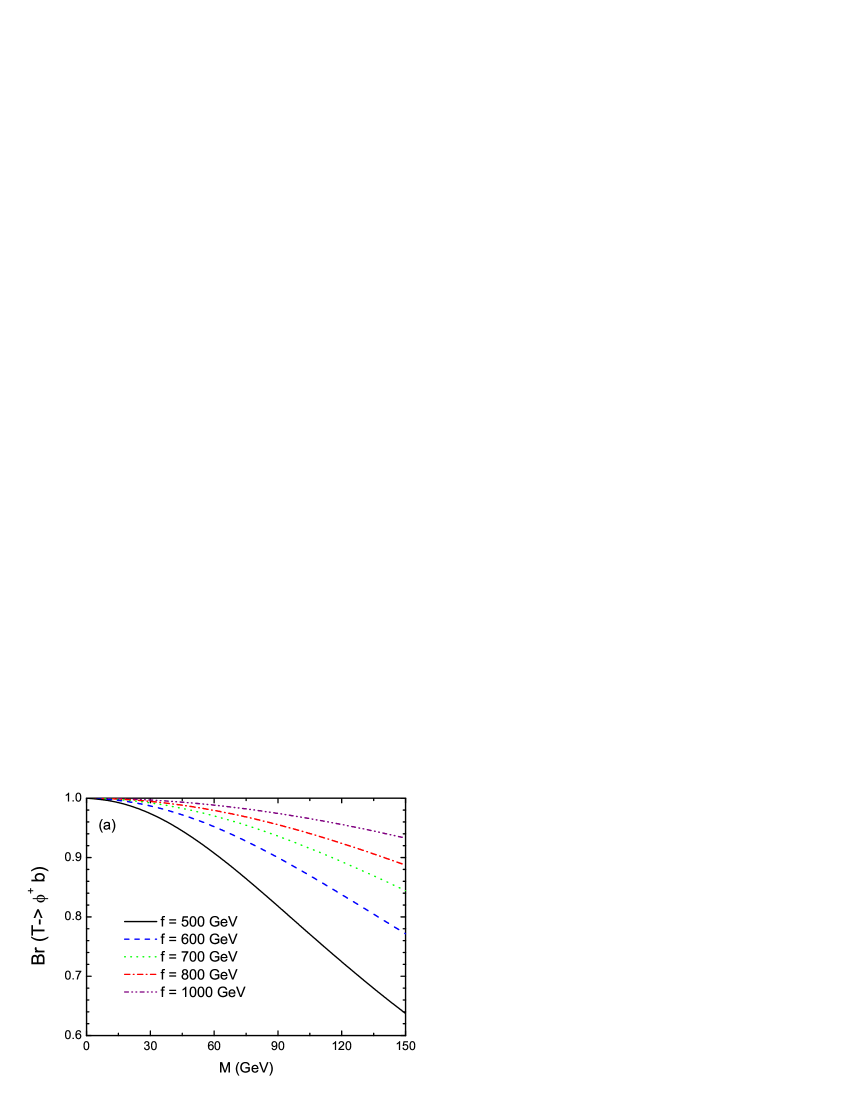
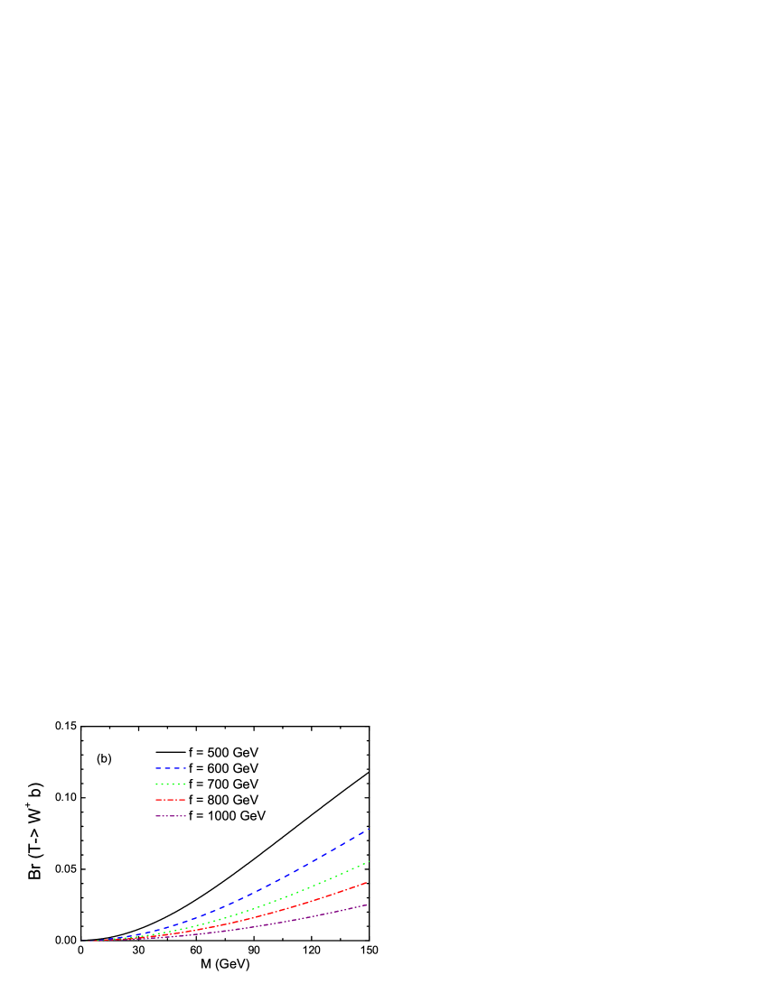
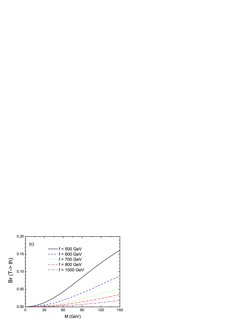
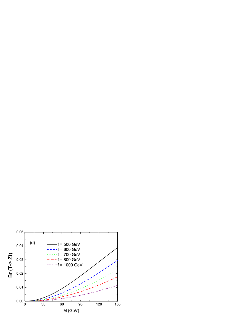
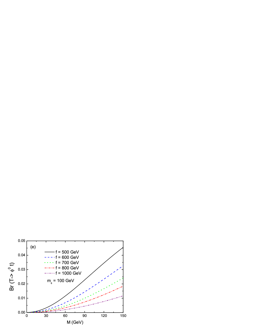
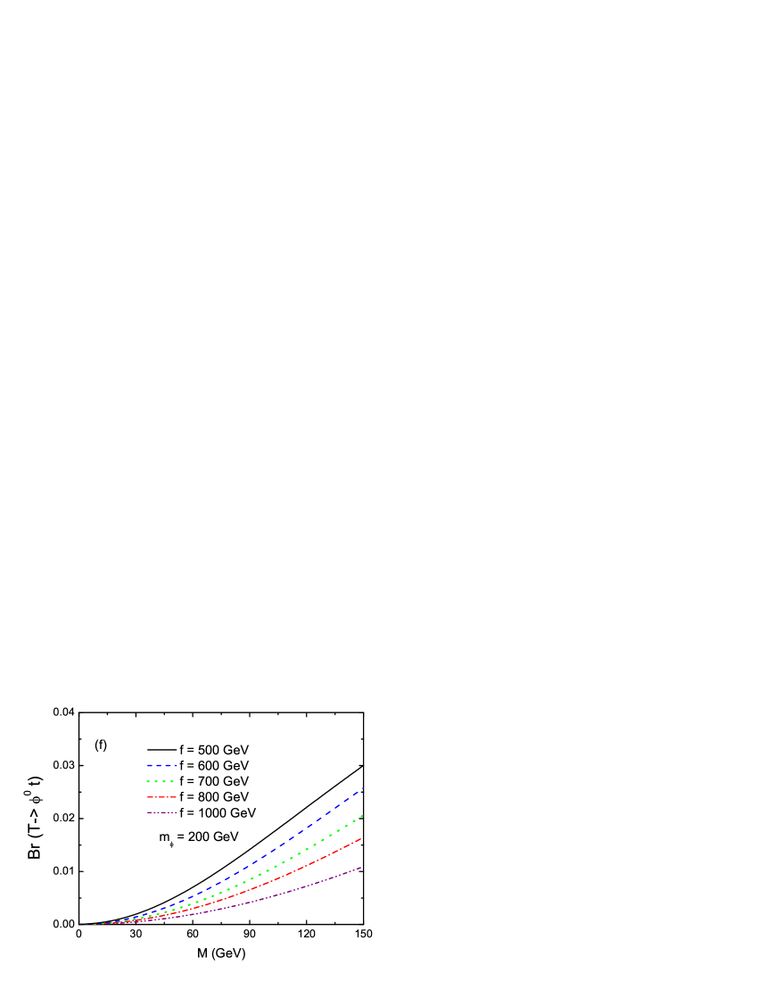
Figure 2: The branching ratios for various $T$ decay modes as a function of the mixing parameter $M$ for five typical values of $f$.

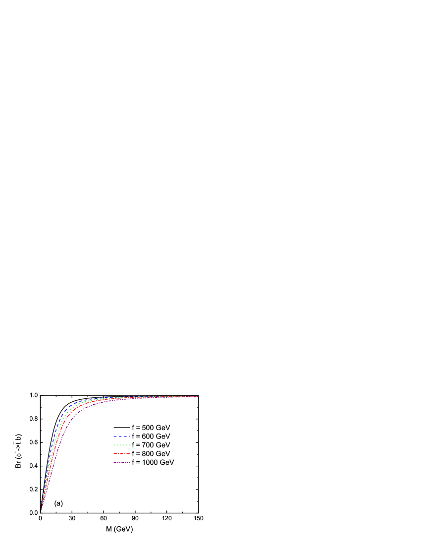
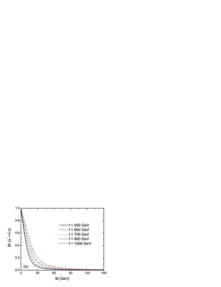
Figure 3: The theoretical predictions for the $M$-dependence of the branching ratios of $\phi^{+}\to t\bar{b}$ and $\phi^{+}\to c\bar{s}$ decays, assuming five typical values of $f$.

In the LRTHM, the charged Higgs $\phi^{\pm}$ decay dominantly into quark pair $tb$ or $cs$ Hock . Fig. 3 shows the LRTHM predictions for the branching ratios for those two decay modes as a function of the the mixing parameter $M$ for five typical values of parameter $f$. One can see from Fig. 3 that the branching ratio of $\phi^{+}\rightarrow t\bar{b}$ decay becomes larger than $50\%$ for large values of $M$. While for very small values of $M$, $\phi^{+}\rightarrow c\bar{s}$ decay dominates, which may lead to completely different phenomenology. For $M=5$ GeV, for example, the branching ratio of $\phi^{+}\rightarrow c\bar{s}$ decay will change from $65.2\%$ to $89.2\%$ when the parameter $f$ increases from 500 GeV to 1000 GeV. In the lower limit $M=0$, the branching ratio of $T\rightarrow c\bar{s}$ is $100\%$.

III Numerical results and discussions

The SM input parameters relevant in our study are taken as $\alpha_{e}=1/128.8$, $S^{2}_{W}=0.2315$, $m_{Z}$=91.187 GeV pdg2012 and $m_{t}$=173.3 GeV topmass . The free LRTHM parameters are $f$ and $M$. Note that the top Yukawa coupling $y$ can be determined by fitting the experimental value of the top quark mass. The masses of top partner and heavy neutral gauge boson can be determined by the value of $f$ and $M$. The typical values of the top partner mass $m_{T}$, the heavy neutral gauge bosons masse $m_{Z_{H}}$ and decay width $\Gamma_{Z_{H}}$ are listed in Table 1 for several benchmark points of the parameter $f$: $f=500,600,700,800,900,1000,1200$ and $f=1500$ GeV.

Table 1: The masses (in GeV) of the top partner $T$, the heavy neutral gauge boson $Z_{H}$ and the total decay width $\Gamma_{Z_{H}}$ used in this paper, assuming $100\leq f\leq 1500$ GeV.

$f$ (GeV)	500	600	700	800	900	1000	1200	1500
$m_{T}(M=0)$	466.4	571.3	674.5	776.8	878.4	979.5	1181	1482
$m_{T}(M=150)$	489.9	590.7	691	791.1	891	991	1190.5	1489.5
$m_{Z_{H}}$	1403	1684	1966	2247	2528	2810	3372	4215
$\Gamma_{Z_{H}}$	29.8	35.7	41.6	47.4	53.3	59.2	71	88.7

In the LRTHM, the phenomenological studies on the signatures of the heavy neutral gauge boson $Z_{H}$ can be found in Ref. lrth-z1 . The present constraints on the $Z^{\prime}$ mass have been presented in pdg2012 . The ATLAS and CMS experiments at the LHC have updated the Tevatron limits on the heavy neutral gauge boson $Z^{\prime}$ mass lhc-z . Recently, the ATLAS and CMS Collaborations presented results on narrow resonances with dilepton final states and excluded a sequential standard model $Z^{\prime}$ with mass smaller than $2.49$ TeV atlas-z and $2.59$ TeV cms-z . Based on the analysis of heavy resonances decaying into $t\bar{t}$ pairs with subsequent fully hadronic and leptonic final states, the ATLAS atlas-ztt and CMS cms-ztt collaborations also excluded the leptophobic $Z^{\prime}$ boson with the mass smaller than $1.32$ TeV (ATLAS) and $1.3$ TeV (CMS). Using constraints from the precision electroweak (EW) data, the lower mass limit on extra neutral boson $Z^{\prime}$ in left-right symmetric models is around $1$ TeV lrsm . Although the Atlas and CMS data have been interpreted in terms of different scenarios for physics beyond the SM, there is no any limit on $Z^{\prime}$ in the LRTHM at present. Our previous study using D0 and CDF results have excluded a $Z^{\prime}$ in the LRTHM with a mass below $940$ GeV lrth-z2 .

The indirect constraints on $f$ come from the $Z$-pole precision measurements, the low energy neutral current process and high energy precision measurements off the $Z$-pole, requiring approximately $f>500$ GeV. On the other hand, it cannot be too large since the fine tuning is more severe for larger $f$. The value of the mixing parameter $M$ is constrained by the $Z\to b\bar{b}$ branching ratio and oblique parameters. Following Ref. Hock , we take the typical parameter space as:

$$500GeV\leq f\leq 1500GeV,\quad 0\leq M\leq 150GeV.$$ (25)

All the numerical studies are done using CalcHEP calchep .

III.1 The single and pair production of top partner

From above discussions, we know that the top partner can be singly or pair produced through $s$-channel gauge bosons exchange by $e^{+}e^{-}$ collisions at ILC and CLIC energies. The relevant Feynman diagrams are depicted in Fig. 4.

Figure 4: Feynman diagrams of the processes $e^{+}e^{-}\to t\overline{T}$ and $e^{+}e^{-}\to T\overline{T}$ in the LRTHM.

III.1.1 The $e^{+}e^{-}\rightarrow t\overline{T}+T\bar{t}$ process

We fist consider the associate production of one top partner $T$ together with the top quark through the $s$-channel $Z$ and $Z_{H}$ exchanges. In Fig. 5a, we plot the production CS $\sigma(e^{+}e^{-}\to t\overline{T}+T\bar{t})$ as a function of the mixing parameter $M$ for $\sqrt{s}=1.5$ TeV and five typical values of $f$. One can see that the cross section decreases as the parameter $f$ increases. This is natural since the phase space is depressed strongly by large $m_{T}$. For $f=600$ GeV and $\sqrt{s}=1.5$ TeV, the maximum of the cross section reaches the level of a few fb. On the other hand, the results also show that the large $M$ can enhance the cross section significantly. In the limit of $M=0$, its value goes to zero.

From Fig. 5b, one can see that the resonance peak of the cross section $\sigma$ emerges when the $Z_{H}$ mass $m_{Z_{H}}$ approaches the c.m. energy. In the region of the resonance peak, the production CSs will be enhanced significantly and can reach the order of pb. For $\sqrt{s}=1.5$ TeV and $f$=700 GeV, for example, the value of $\sigma$ is about $5$ fb. If we assume that the future ILC experiment with $\sqrt{s}$=1.5 TeV has a yearly integrated luminosity of 500fb^-1, then there will be several thousand signal events generated at the ILC.

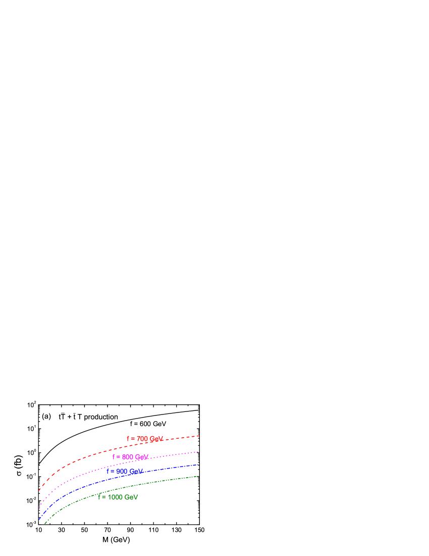
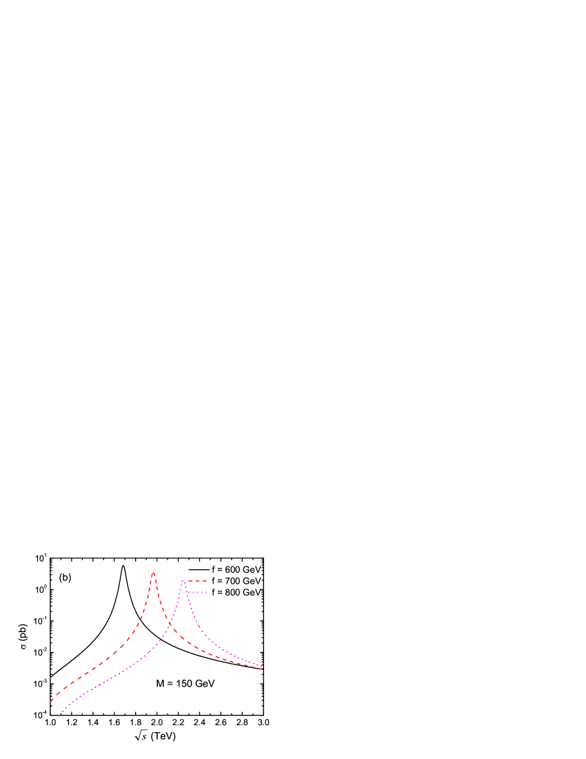
Figure 5: (a) The production CS $\sigma$ as a function of the mixing parameter $M$ for $\sqrt{s}=1.5$ TeV and $f=600,700,800,900$, and 1000 GeV; (b)The production CS $\sigma$ as a function of center of mass energy $\sqrt{s}$ for $M=150$ GeV and three values of $f$ as indicated.

For a large value of $M$, the dominate subsequent decay of $T\to\phi^{+}b$ and $\phi^{+}\to t\bar{b}$ make the process $e^{+}e^{-}\to t\overline{T}+T\bar{t}$ mainly decaying to the final state $t\bar{t}b\bar{b}$. The production rates for such final states can be easily estimated as

$$\sigma\times\Bigl{[}Br(T\to\phi^{+}b)\cdot Br(\phi^{+}\to t\bar{b})+Br(T\to th)\cdot Br(h\to b\bar{b})$$

$$\hskip 56.9055pt+Br(T\to tZ)\cdot BR(Z\rightarrow b\bar{b})+Br(T\rightarrow t\phi^{0})\cdot Br(\phi^{0}\rightarrow b\bar{b})\Bigr{]}.$$ (26)

For the semi-leptonic decays of $t\bar{t}$, the characteristic collider signal is two jet + four b + one lepton ($e$ or $\mu$) + missing $\hbox to0.0pt{\hskip 0.56917pt/\hss}{E_{T}}$. The dominant SM background processes and their production CS’s with $\sqrt{s}=1.5$ TeV are listed in Table 2. The backgrounds $t\bar{t}h$ and $t\bar{t}Z$ are also included when $t\bar{t}b\bar{b}$ is estimated. We can see that the total background CS is about 0.4 fb. Note that these numerical results are estimated by using MadGraph mad and cross-checked with CalcHEP without considering any kinematical cuts and tagging efficiency.

Table 2: The possible SM background CS’s (in fb) in semi-leptonic channel ($2j+4b+\ell+\hbox to0.0pt{\hskip 0.56917pt/\hss}{E_{T}}$) are estimated with $\sqrt{s}=1.5$ TeV. We used $Br(t\rightarrow W^{+}b)=1$, $Br(W^{\pm}\rightarrow jj^{\prime})=0.68$, $Br(W^{\pm}\rightarrow\ell^{\pm}\nu_{l})=0.107$, $Br(h\rightarrow b\bar{b})=0.57$ and $Br(Z\rightarrow b\bar{b})=0.15$.

Processes	Cross sections (fb)
$e^{+}e^{-}\rightarrow t\bar{t}b\bar{b}$	$\sigma(e^{+}e^{-}\rightarrow t\bar{t}b\bar{b}\rightarrow 2j+4b+\ell+\hbox to0.0pt{\hskip 0.56917pt/\hss}{E_{T}})=0.4$
$e^{+}e^{-}\rightarrow W^{+}W^{-}ZZ$	$\sigma(e^{+}e^{-}\rightarrow W^{+}W^{-}ZZ\rightarrow 2j+4b+\ell+\hbox to0.0pt{\hskip 0.56917pt/\hss}{E_{T}})=0.006$
$e^{+}e^{-}\rightarrow W^{+}W^{-}hh$	$\sigma(e^{+}e^{-}\rightarrow W^{+}W^{-}hh\rightarrow 2j+4b+\ell+\hbox to0.0pt{\hskip 0.56917pt/\hss}{E_{T}})=0.008$
$e^{+}e^{-}\rightarrow W^{+}W^{-}Zh$	$\sigma(e^{+}e^{-}\rightarrow W^{+}W^{-}Zh\rightarrow 2j+4b+\ell+\hbox to0.0pt{\hskip 0.56917pt/\hss}{E_{T}})=0.002$

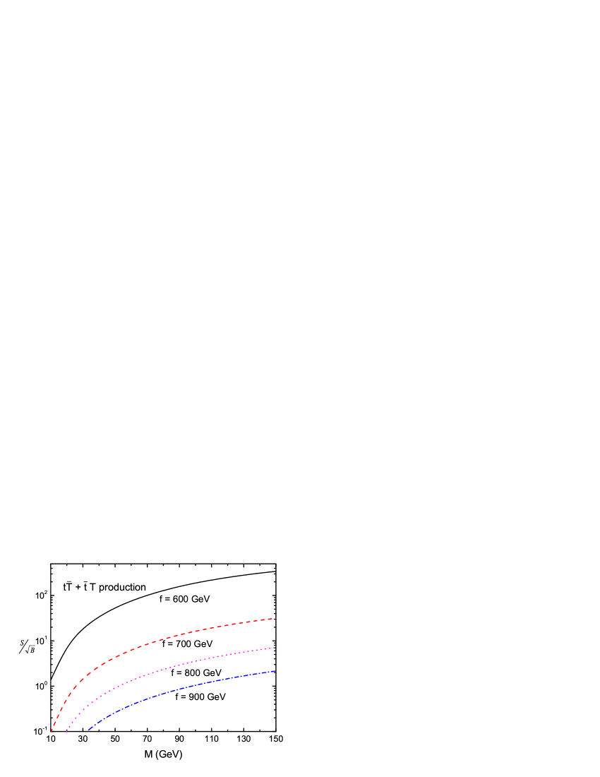
Figure 6: The statistical significance $S/\sqrt{B}$ as a function of the the mixing parameter $M$ for $\sqrt{s}=1.5$ TeV and four typical values of $f$.

In order to discuss the observation of the top partner, we calculate the statistical significance $S/\sqrt{B}$ ($S$ denotes the signal and $B$ the SM background) and the numerical results are shown in Fig. 6, here we assumed that the integrated luminosity is $500$ fb^-1. One can see that, for large $M$ and small $f$, the value of the statistical significance $S/\sqrt{B}$ is larger than 5. For $f\geq 600$ GeV, the mass of the heavy gauge boson is larger than 1680 GeV and the resonance peak will not appear. Consequently, it may be possible to extract the signals from the backgrounds in the reasonable parameter space of the LRTHM.

It is obvious that this is only a simple estimate. To take into account detector acceptance we should consider the tagging efficiency and some appropriate kinematical cuts. On the other hand, the reconstruction of the top partner and the charged Higgs bosons is very necessary to distinguish the signal from the background. In our estimates, we have excluded the efficiency $\epsilon_{b}^{4}$ of tagging the four $b$-jets in the final state. If we take the single $b$-tagging efficiency as about $70\%$, as one would expect, after putting some basic acceptance cuts required to trigger on the final states, the rates would become smaller. However, our main conclusions should remain unchanged. Obviously, the detailed analysis for individual processes would require Monte-Carlo simulations of the signals and backgrounds, which is beyond the scope of the current paper.

III.1.2 The $e^{+}e^{-}\to T\overline{T}$ process

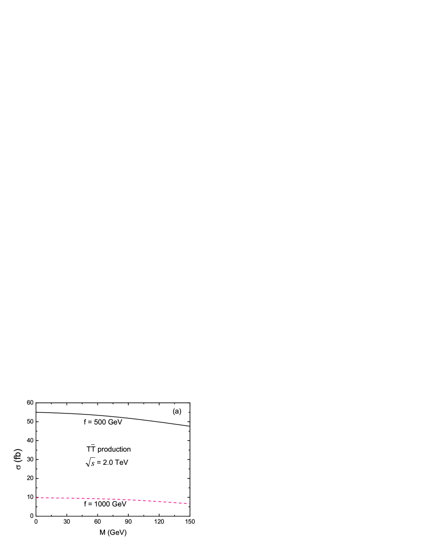
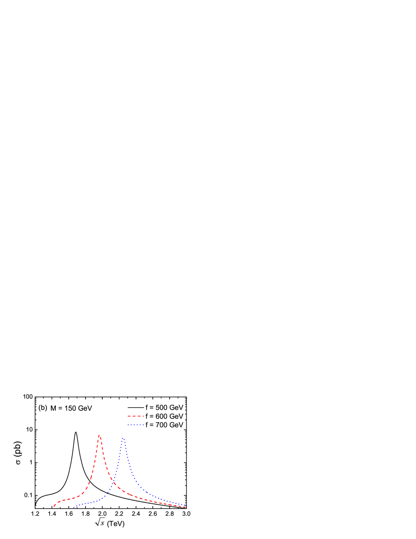
Figure 7: (a) The production CS $\sigma$ as a function of the mixing parameter $M$ for $\sqrt{s}=2.0$ TeV and $f=500$GeV and 1000 GeV; (b) The production CS $\sigma$ as a function of center of mass energy $\sqrt{s}$ for $M=150$ GeV and three values of $f$ as indicated.

We next consider the pair production of the top partner $T$ at the CLIC. The production CS’s $\sigma$ are plotted as a function of the mixing parameter $M$ in Fig. 7a and as a function of $\sqrt{s}$ in Fig. 7b for various typical values of $f$. From Fig. 7a, one can see that the cross section is insensitive to the parameter $M$. For $f=500$ GeV, for example, the cross section $\sigma$ is changing from $55$ fb to $48$ fb when the parameter $M$ increases from 0 to 150 GeV. In the most of the parameter spaces, the production CS are at the level of tens of fb for $\sqrt{s}=2.0$ TeV. However, one can see from Fig. 7b that the resonance peak of the $\sigma$ can reach a few pb when $M_{Z_{H}}\simeq\sqrt{s}$, provided that the LHC measures the masses of the extra gauge bosons predicted by the LRTHM. For $\sqrt{s}=3$ TeV this resonance scan can be extended to upper values of the scale $f$ around 1.1 TeV.

Considering the subsequent decay of the top partner $T$, the characteristic signal of $T\overline{T}$ events might be:

• Case I: One lepton ($e$ or $\mu)$ + two jets +6b + missing $\hbox to0.0pt{\hskip 0.56917pt/\hss}{E_{T}}$, which arises from the decay modes $\phi^{+}b$, $ht$, $Zt$, and $\phi^{0}t$ of the top partner $T$ with the cascade decays $\phi^{+}\to t\bar{b}$, $t\to W^{+}b$, $h\to b\bar{b}$, $Z\to b\bar{b}$ and $\phi^{0}\to b\bar{b}$, and the subsequent decay of one $W$ bosons through leptonic decay channel and others in their hadronic decays.

• Case II: Four jets +$2b$, which happens for a very small value of $M$ with $T\to\phi^{+}b$ and $\phi^{+}\to c\bar{s}$, eg., $M=0$.

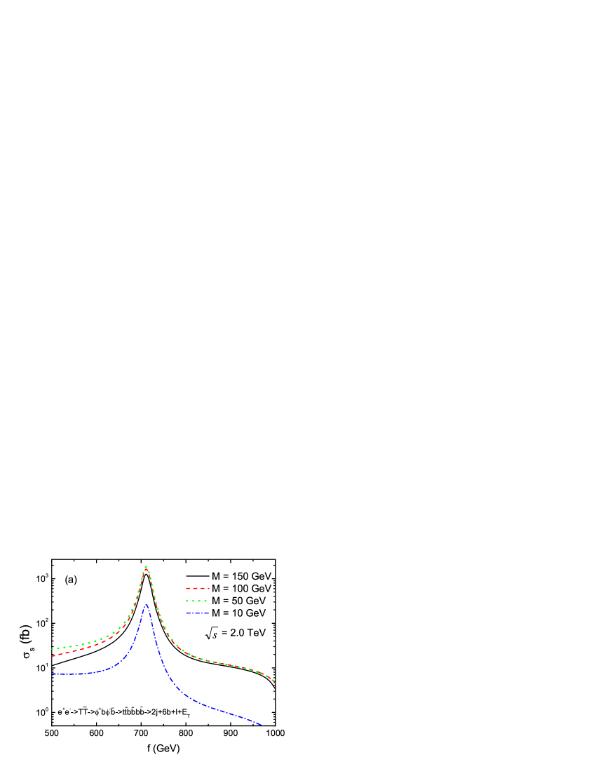
Figure 8: (a) The production rates of the $2j+6b+\ell+\hbox to0.0pt{\hskip 0.56917pt/\hss}{E_{T}}$ final state as a function of $f$ for $\sqrt{s}=2.0$ TeV and four typical values of $M$ as indicated; (b) The production rates of the $4j+2b$ final state as a function of $f$ for $\sqrt{s}=2.0$ TeV and $M=0$.

For $\sqrt{s}=2.0$ TeV, the total production rates of the signals for above two cases are shown in Fig. 8. For Case I, the production rate of the signal can reach tens of fb except for the resonance effect, as shown in Fig. 8a. While for case II, the production rate of the signal are higher about one order than that for Case I with the same value of parameter $f$, as shown in Fig. 8b. For $f=600$ GeV and $M=0,150$ GeV, the production rates for two cases are about 161 fb and 24 fb, respectively. If we assume that the future CLIC experiment with $\sqrt{s}$=2.0 TeV has a yearly integrated luminosity of 500fb^-1, then there will be about $10^{4}$ signal events generated per year.

For above two kinds of signals the possible backgrounds from the SM processes are listed in Table 3. For Case I, one can see that the background are much smaller than the signal. With the signal CS and the expected CLIC high luminosity, one can easily get large number of events even if we lose some of events by imposing cuts to remove SM backgrounds.

Table 3: The SM background CS’s (in fb) for $2j+6b+\ell+\hbox to0.0pt{\hskip 0.56917pt/\hss}{E_{T}}$ (Case I) and $4j+2b$ (Case II) final states, estimated with $\sqrt{s}=2.0$ TeV.

Case I
$\sigma(e^{+}e^{-}\to t\bar{t}Zh)=0.04$	$\sigma(e^{+}e^{-}\to t\bar{t}ZZ\to 2j+6b+l+\hbox to0.0pt{\hskip 0.56917pt/\hss}{E_{T}})=9.8\times 10^{-4}$
$\sigma(e^{+}e^{-}\to t\bar{t}hh)=0.011$	$\sigma(e^{+}e^{-}\to t\bar{t}hh\to 2j+6b+l+\hbox to0.0pt{\hskip 0.56917pt/\hss}{E_{T}})=1.02\times 10^{-3}$
$\sigma(e^{+}e^{-}\to t\bar{t}ZZ)=0.056$	$\sigma(e^{+}e^{-}\to t\bar{t}ZZ\to 2j+6b+l+\hbox to0.0pt{\hskip 0.56917pt/\hss}{E_{T}})=3.7\times 10^{-4}$
Case II
$\sigma(e^{+}e^{-}\to t\bar{t})=43.8$	$\sigma(e^{+}e^{-}\to t\bar{t}\to W^{+}bW^{-}\bar{b}\to 4j+2b)=20.3$
$\sigma(e^{+}e^{-}\to W^{+}W^{-}Z)=43.4$	$\sigma(e^{+}e^{-}\to W^{+}W^{-}Z\to 4j+2b)=3.01$
$\sigma(e^{+}e^{-}\to W^{+}W^{-}h)=1.8$	$\sigma(e^{+}e^{-}\to W^{+}W^{-}h\to 4j+2b)=0.47$
$\sigma(e^{+}e^{-}\to ZZb\bar{b})=0.19$	$\sigma(e^{+}e^{-}\to ZZb\bar{b}\to 4j+2b)=0.09$
$\sigma(e^{+}e^{-}\to ZZh)=0.13$	$\sigma(e^{+}e^{-}\to ZZh\to 4j+2b)=0.04$
$\sigma(e^{+}e^{-}\to ZZZ)=0.5$	$\sigma(e^{+}e^{-}\to ZZZ\to 4j+2b)=0.04$

For Case II, the large background comes from the SM process $e^{+}e^{-}\to t\bar{t}\to 2W+2b\to 4j+2b$ with the cross section about 20 fb. Since the cross sections of the SM processes are not too large compared to the signal process, the reconstruction of top partner $T$ and the charged Higgs bosons $\phi^{+}$ is necessary to distinguish the signal from the background. For example, one must first search for the hadronic decay of a charged Higgs boson by choosing the combination which minimizes $|m_{jj}-m_{\phi}|$. An apparent feature of difference between signal and the background is that the di-jet invariant mass for the background events primarily reconstructs to $m_{W}$ but the di-jet invariant mass for the signals coming from the charged Higgs approaches $m_{\phi}$. Such difference can help us to distinguish the signals from the background. Secondly, each top partner $T$ is reconstructed from one charged Higgs candidate paired with one of the two $b$ jets, such that the invariant masses of the $\phi^{+}b$ systems are as close as possible to top partner mass.

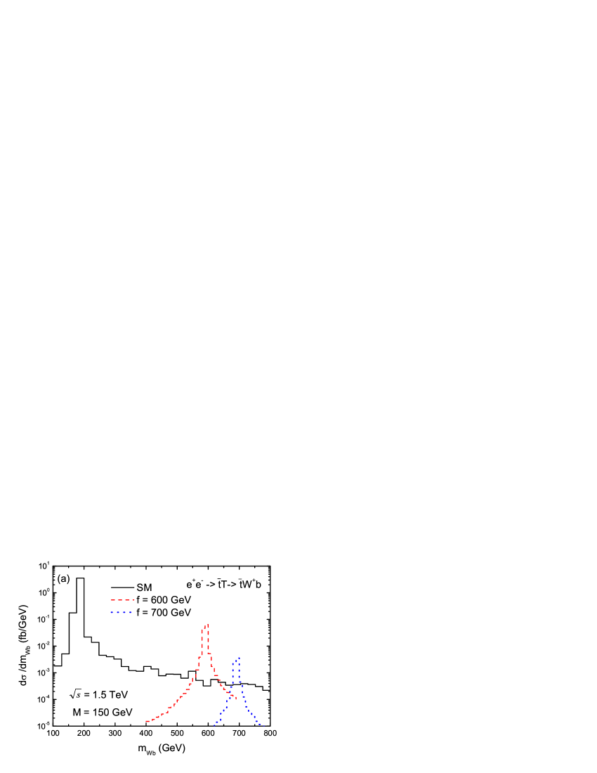
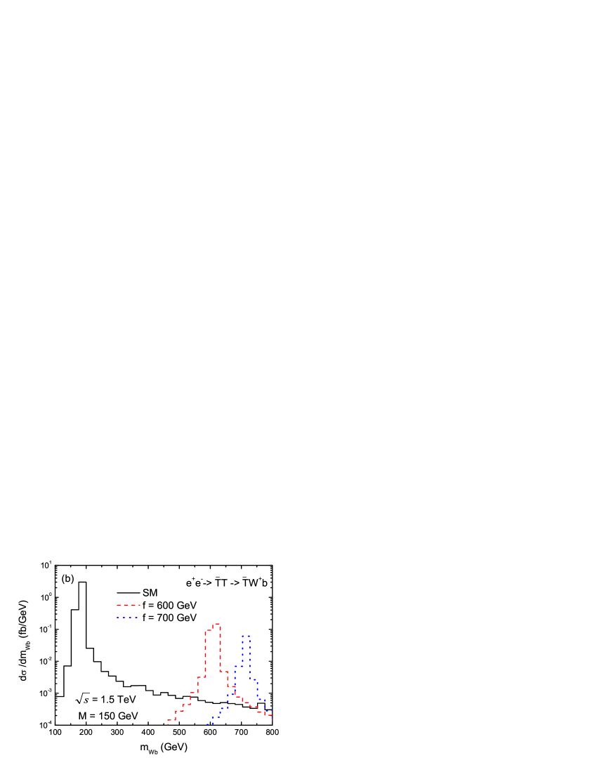
Figure 9: The invariant mass distributions for the SM background and the $Wb$ signal from $T$ decay for (a) $e^{+}e^{-}\to\bar{t}T\to\bar{t}W^{+}b$ and (b) $e^{+}e^{-}\to\overline{T}T\to\overline{T}W^{+}b$.

For the decay channel $T\to W^{+}b$, the top partner production can give rise to the same final state as the SM top quark. The leptonic $W$ decay yields a nice signal of one $b$ jet plus one electron or muon with missing energy. For $M=150$ GeV and $f=600,700$ GeV, the branching ratios of $T\to W^{+}b$ are about $7.8\%$ and $5.5\%$, respectively. The invariant mass distributions for the SM background and the $Wb$ signal from $T$ decay are shown in Fig. 9 for two processes with $\sqrt{s}=1.5$ TeV and $M=150$ GeV. It is clear that the $T$-quark signal can be observed as a resonance in the $W^{+}b$ invariant mass distribution at the CLIC.

III.2 Associate productions of $T$ with SM-like Higgs boson $h$

Like $ht\bar{t}$ production, the productions of $ht\overline{T}$ can also be realized at the linear $e^{+}e^{-}$ collider, as shown in Fig. 10. Thus, it is possible to measure the Yukawa coupling between top partner and other particles simply by measuring the production CS’s of the relevant processes with high center of mass energy. There are two SM-like Higgs boson associated production processes. One is the Higgs production associating with a top quark and a top partner production $e^{+}e^{-}\to t\overline{T}h(T\bar{t}h)$, and another is the process associating with top partner pairs $e^{+}e^{-}\to T\overline{T}h$. Here we fixed the SM-like Higgs boson mass as $m_{h}=125.5$ GeV. Considering the dominant decay mode $T\to\phi^{+}b\to t\bar{b}b$, the $t\overline{T}h$ and $T\overline{T}h$ production processes have less background than $ht\bar{t}$ production and these new production channels at the LHC have been studied in sjf .

Figure 10: Typical Feynman diagrams of the process $e^{+}e^{-}\to t\overline{T}h$ in the LRTHM.

III.2.1 The $e^{+}e^{-}\to t\overline{T}h+T\bar{t}h$ process

We first consider the Higgs production process associated with a top quark and a top partner. The sum of the CS, $\sigma(e^{+}e^{-}\to t\overline{T}h)+\sigma(e^{+}e^{-}\to T\bar{t}h)$, are shown in Fig. 11. One can see that in the major region of the parameter space, the CS are at the level of several fb for $M=150$ GeV. For example, the CS is about 3.6 fb for $\sqrt{s}=1.5$ TeV and $f=700$ GeV. On the other hand, the resonance peak values of the $\sigma$ can reach the order of $10^{2}$ fb. The production CS is, furthermore, very sensitive to the parameter $M$: large values of $M$ can enhance the CS significantly. This is due to the couplings of $t\overline{T}h$, $Zt\overline{T}$ and $Z_{H}t\overline{T}$ are all proportional to the factor $(M/f)$. In the limit of $M=0$, all theses couplings are vanishing. For $\sqrt{s}=3$ TeV, $f$=1200 GeV, the value of $\sigma$ is changing from $0.02$ fb to $0.42$ fb when the parameter $M$ increases from 30 GeV to 150 GeV.

Figure 11: (a) The production CS $\sigma$ as a function of $\sqrt{s}$ for $M=150$ GeV and three values of $f$ as indicated; (b) The production CS $\sigma$ as a function of the mixing parameter $M$ for $\sqrt{s}=3.0$ TeV and $f=600,800,1200,1400$ GeV respectively.

For a large value of $M$, the dominate decay mode $h\to b\bar{b}$ will lead to the cascade decay chain $e^{+}e^{-}\to t\overline{T}h+T\bar{t}h\to t\bar{t}b\bar{b}b\bar{b}$. The production rates for the final state $t\bar{t}b\bar{b}b\bar{b}$ can be easily estimated:

$$\sigma_{s} \simeq \sigma\times\Bigl{[}Br(T\to\phi^{+}b)\cdot Br(\phi^{+}\to t\bar{b})+Br(T\to th)\cdot Br(h\to b\bar{b})$$ (27)

$$+Br(T\to tZ)\cdot BR(Z\to b\bar{b})+Br(T\to t\phi^{0})\cdot Br(\phi^{0}\to b\bar{b})\Bigr{]}.$$

In Table 4 we present the total CS for the final states $t\bar{t}b\bar{b}b\bar{b}$ via the process $e^{+}e^{-}\to t\overline{T}h+T\bar{t}h$ with $\sqrt{s}=3.0$ TeV and various parameter values. The main backgrounds for the $t\bar{t}b\bar{b}b\bar{b}$ final state come from the SM processes $e^{+}e^{-}\to t\bar{t}ZZ$, $e^{+}e^{-}\to t\bar{t}Zh$ and $e^{+}e^{-}\to t\bar{t}hh$ with $Z\to b\bar{b}$ and $h\to b\bar{b}$, continuum $t\bar{t}b\bar{b}b\bar{b}$ production. The total CS of the SM backgrounds is estimated about 0.01 fb, which is smaller than that in the signal. Thus, it may be possible to extract the signals from the backgrounds in the reasonable parameter spaces in the LRTHM (eg., for large $M$ and small $f$).

Table 4: The total CS’s (in fb) of signal for the final states $t\bar{t}b\bar{b}b\bar{b}$ with $\sqrt{s}=3.0$ TeV.

$f$ (GeV)	600	800	1200	1400
$M=50$ GeV	0.42	0.23	0.047	0.013
$M=100$ GeV	1.43	0.87	0.21	0.053
$M=150$ GeV	2.56	1.53	0.4	0.12

III.2.2 The $e^{+}e^{-}\to T\overline{T}h$ process

Figure 12: (a) The production CS $\sigma$ as a function of $\sqrt{s}$ for four values of $M$ as indicated and $f=700$ GeV; (b)The production CS $\sigma$ as a function of the mixing parameter $M$ for $\sqrt{s}=2.0$ TeV and four typical values of $f$ as indicated.

Next, we consider the pair production of the top partner $T$ associated with the Higgs boson: $e^{+}e^{-}\to T\overline{T}h$. In Fig. 12a, we show its production CS versus $\sqrt{s}$ with various $M$ for $f=700$ GeV. One can see that the resonance CS’s are at the level of several fb. In the most parameter space, the CS’s are smaller than 0.1 fb. From Fig. 12b one can see that the CS decrease along with the increase of $f$, and is also insensitive to the variation of $M$. For $f=800$ GeV, the CS $\sigma$ is changing from $0.03$ fb to $0.025$ fb when the parameter $M$ increases from 0 to 150 GeV.

Similar to the character of $e^{+}e^{-}\to T\overline{T}$ process, the characteristic signal of $T\overline{T}h$ with $h\to b\bar{b}$ might be

• Case A: $2j+8b+\ell+\hbox to0.0pt{\hskip 0.56917pt/\hss}{E_{T}}$ for $M=150$ GeV, which arises from the semi-leptonic decays of the $t\bar{t}$ system.

• Case B: $4j+4b$ in the limit of $M=0$, which arises from $T\to\phi^{+}b$ and $\phi^{+}\to c\bar{s}$ with the branching ratios of $100\%$.

Table 5: The possible signal cross sections (in fb) for above two cases are estimated with $\sqrt{s}=2.0$ TeV.

Signals	$f=600$ GeV	$f=800$ GeV	$f=900$ GeV
Case A	$1.4\times 10^{-2}$	$3.3\times 10^{-3}$	$5.6\times 10^{-4}$
Case B	$9.6\times 10^{-2}$	$1.8\times 10^{-2}$	$3.5\times 10^{-3}$

The CS’s of possible signals are listed in Table 5 with $\sqrt{s}=2.0$ TeV. The reducible SM backgrounds for Case A are almost negligible. Given a sufficient integrated luminosity, it may be possible to detect these signals in the reasonable parameter space of the LRTH model, especially for small value of $f$. The main background processes for the Case B have been extensively studied in tth1 ; tth2 by applying the suitable cuts. According their conclusions, we have to say that it is very difficult to discriminate the $4j+4b$ signal due to the low production rates, low selection efficiencies and large SM background.

III.3 Associate production with $\phi^{0}$

Figure 13: Feynman diagrams of the process $e^{+}e^{-}\to T\bar{t}\phi^{0}$ in the LRTHM.

Besides the SM-like Higgs boson $h$, the LRTHM also predicts the existence of the neutral pseudoscalar boson $\phi^{0}$. In Ref. liu-jhep , we studied the production and decays of a light $\phi^{0}$. The relevant couplings can be written as Hock :

$$\phi^{0}\overline{T}t : -iy(S_{L}C_{R}P_{L}-C_{L}S_{R}P_{R})/\sqrt{2},$$

$$\phi^{0}T\overline{T} : -iyC_{L}C_{R}\gamma_{5}/\sqrt{2},$$

$$h\phi^{0}Z_{\mu} : iexp3_{\mu}/(6s_{W}c_{W}),$$

$$h\phi^{0}Z_{H\mu} : iex[(14-17s_{W}^{2})p2_{\mu}-(4-s_{W}^{2})p1_{\mu}]/(18s_{W}c_{W}\sqrt{1-2s_{W}^{2}}),$$ (28)

where $P_{L,R}=(1\mp\gamma_{5})/2$, $p1$, $p2$ and $p3$ refer to the incoming momentum of the first, second and third particle, respectively. It is easy to see that the top partner $T$ can be produced via the process $e^{+}e^{-}\to\phi^{0}T\bar{t}$, as shown in Fig. 13. Similarly, the associated production of $\phi^{0}t\overline{T}$ and $\phi^{0}T\overline{T}$ can also happen although we do not show them explicitly in Fig. 13.

III.3.1 The $e^{+}e^{-}\to t\overline{T}\phi^{0}+T\bar{t}\phi^{0}$ process

In Fig. 14, we plot the parameter dependence of the summation of the production CS, $\sigma(e^{+}e^{-}\to t\overline{T}\phi^{0})+\sigma(e^{+}e^{-}\to T\bar{t}\phi^{0})$. This case is similar to those in the SM-like Higgs boson associate production processes. One can see that in the considered parameter space, the production CS are at the level of several fb for $M=150$ GeV. The resonance peak values of the $\sigma$ can reach the order of $10^{2}$ fb. On the other hand, the production CS is very sensitive to the parameter $M$ and decreases along with the increase of $m_{\phi^{0}}$. For $\sqrt{s}=2.0$ TeV, $f$=600 GeV and $m_{\phi^{0}}=120$ GeV, the value of $\sigma$ is changing from $0.26$ fb to $4.2$ fb when the parameter $M$ increases from 30 GeV to 150 GeV. Thus, a large value of $M$ can enhance the production rates for this process.

Figure 14: (a) The production CS as a function of $\sqrt{s}$ for $M=150$ GeV, $m_{\phi^{0}}=120$ GeV and $f=600,900$ GeV; (b) The production CS $\sigma$ as a function of the mixing parameter $M$ for $\sqrt{s}=2.0$ TeV, $f=600$ GeV, and $m_{\phi^{0}}=50,120$ GeV.

The dominant decay mode of $\phi^{0}$ is $\phi^{0}\to b\bar{b}$, with a branching ratio $Br(\phi^{0}\to b\bar{b})\simeq 0.8$ fb for $m_{\phi^{0}}=120$ GeV liu-jhep . For a large value of $M$, the dominate decay mode $T\to\phi^{+}b\to t\bar{b}b$ can also make the process $e^{+}e^{-}\to t\overline{T}\phi^{0}+T\bar{t}\phi^{0}$ also give rise to the $t\bar{t}b\bar{b}b\bar{b}$ final state, which is similar to the case of $(t\overline{T}h+T\bar{t}h)$ productions. The branching ratio for the $t\to bW^{+}$ is essentially one which induced to the final state of $6b+2W$. Now we consider one $W$ boson decay hadronically and the other decay leptonically. Thus the resulting final state signal is $2j+6b+\ell+\hbox to0.0pt{\hskip 0.56917pt/\hss}{E_{T}}$. The production rates of such final state are shown in Table 6 with $m_{\phi^{0}}=120$ GeV, $\sqrt{s}=2.0$ TeV and various parameter values. For $f=600$ GeV and $M=150$ GeV, there will be about 230 signal events with a yearly integrated luminosity of 500fb^-1. The relevant SM backgrounds for this final state is negligible. Note that what we have presented here as an estimate of the signal events is just a rude estimate. If we take the $b$-tagging efficiency of each of the six $b$ quarks which is about $70\%$, the estimated event rates are suppressed about $(0.7)^{6}\simeq 0.12$ and this still gives us tens of observable events for the signal with high luminosity. Thus, it may be possible to extract the signals from the backgrounds due to the large production rates in the reasonable parameter spaces of the LRTHM.

Table 6: The total cross sections (in fb) of signal for the final states $2j+6b+\ell+\hbox to0.0pt{\hskip 0.56917pt/\hss}{E_{T}}$ in the LRTHM for $m_{\phi^{0}}=120$ GeV and $\sqrt{s}=2.0$ TeV.

$M$ (GeV)	30	60	90	120	150
f=600 GeV	0.03	0.11	0.26	0.39	0.46
f=900 GeV	0.003	0.012	0.028	0.045	0.074

III.3.2 The $e^{+}e^{-}\to T\overline{T}\phi^{0}$ process

Figure 15: (a) The production CS $\sigma$ as a function of $\sqrt{s}$ for $M=150$ GeV, $m_{\phi^{0}}=120$ GeV and three values of $f$ as indicated; (b)The production CS $\sigma$ as a function of the mixing parameter $M$ for $\sqrt{s}=2.0$ TeV, $f=600$ GeV, and $m_{\phi^{0}}=50,120$ GeV.

The production CS of the process $e^{+}e^{-}\to T\overline{T}\phi^{0}$ are shown in Fig. 15. One can see that the resonance CS’s can reach the level of 1 fb. Apart from the resonance peak, the cross sections are smaller than 0.1 fb in the most parameter space. For $f=600$ GeV, $m_{\phi^{0}}=120$ GeV and $\sqrt{s}=2.0$ TeV, the cross section $\sqrt{s}$ is changing from $0.084$ fb to $0.066$ fb when the parameter $M$ increases from 0 to 150 GeV. Thus, it is challenging to detect the signals of top partner via this production process due to the small production rates, except for the resonant region.

IV Conclusions

The LRTHM predicts the existence of the top partner $T$ which may be observable at the high energy linear $e^{+}e^{-}$colliders. In this paper, we study the single and pair production of the top partner at the ILC and CLIC via the processes: $e^{+}e^{-}\to(t\overline{T},T\bar{t},T\overline{T})$, the Higgs boson $h$ associate productions $e^{+}e^{-}\to(t\overline{T}h,T\bar{t}h,T\overline{T}h)$, and the neutral pseudoscalar boson associate productions $e^{+}e^{-}\to(t\overline{T}\phi^{0},T\bar{t}\phi^{0})$ and $e^{+}e^{-}\to T\overline{T}\phi^{0}$. From the numerical calculations and the phenomenological analysis for all considered production and decay modes, we find the following observations:

1. The top partner $T$ mainly decay into $\phi^{+}b$ with the branching ratio larger than $60\%$ for 500 GeV $\leq f\leq$1000 GeV, while the branching ratio of $T\to Wb$ mode is about $11\%$ for $M=150$ GeV and $f$=500 GeV. The current bound on the top partner mass $m_{T}$ could be relaxed.

2. For the single top partner production processes: $T\bar{t}$, $T\bar{t}h$, and $T\bar{t}\phi^{0}$, the production CS’s are sensitive to the mixing parameter $M$, and will increase when the mixing parameter $M$ becomes larger. Except for the resonance regions, the production CS’s can reach the level of several fb for $M=150$ GeV.

3. For the pair production process $e^{+}e^{-}\to T\overline{T}$, the production CS’s are insensitive to the mixing parameter $M$, and the production CS’s can reach the level of tens of fb. However, the production CS’s of the processes $e^{+}e^{-}\to T\overline{T}h$ and $e^{+}e^{-}\to T\overline{T}\phi^{0}$ are smaller than 0.1 fb in the major part of the parameter space in the LRTHM.

4. For the cases of the resonant production, the position and the shape of the peak of the production CS have strong dependence of the value of the parameter $f$. The subsequent decay of $T\to\phi^{+}b$, $\phi^{+}\to t\bar{b}$, $t\to W^{+}b$ and $W\to\ell\nu$ can give rise to the signal of the top partner $T$ with the $3b+\ell+\hbox to0.0pt{\hskip 0.56917pt/\hss}{E_{T}}$, which can generate typical phenomenological features for the top partners in the LRTHM.

5. According to our SM background analysis, we get to know that the signal of the top partner $T$ predicted by the LRTHM, in the reasonable parameter space ( say small $f$ and large $M$), may be detectable in the future ILC and CLIC experiments.

- (1) G. Aad et al., [ATLAS Collaboration], Phys.Lett. B 716,1 (2012); Phys.Lett. B 726, 120 (2013).
- (2) S. Chatrchyan et al., [CMS Collaboration], Phys.Lett. B 716, 30 (2012).
- (3) C.S. Li, H.T. Li and D.Y. Shao, Chin. Sci. Bull. 59, 3709 (2014), and references therein.
- (4) X.P. Wang and S.H. Zhu, Chin. Sci. Bull. 59, 3729 (2014).
- (5) R. Barbieri and A. Strumia, Phys.Lett. B 462, 144 (1999).
- (6) Z. Chacko, H.S. Goh and R. Harnik, Phys.Rev.Lett. 96, 231802 (2006); Z. Chacko, Y. Nomura, M. Papucci and G. Perez, J. High Energy Phys. 0601, 126 (2006); A. Falkowski, S. Pokorski and M. Schmaltz, Phys.Rev. D 74, 035003 (2006).
- (7) H.S. Goh and C.A. Krenke, Phys.Rev. D 76, 115018(2007).
- (8) Z. Chacko, H.S. Goh and R. Harnik, J. High Energy Phys. 0601, 108 (2006).
- (9) H.S. Goh and S.F. Su, Phys.Rev. D 75, 075010 (2007).
- (10) A. Abada and I. Hidalgo, Phys.Rev. D 77,113013 (2008); E.M. Dolle and S.F. Su, Phys.Rev. D 77,075013 (2008); P. Batra and Z. Chacko, Phys.Rev. D 79, 095012 (2009).
- (11) L. Wang, J.M. Yang, J. High Energy Phys. 1005, 024 (2010); L. Wang, X.F. Han, Phys.Lett. B 696, 79 (2011).
- (12) Y.B. Liu, H.M. Han and X.L. Wang, Eur.Phys.J. C 53, 615 (2008); Y.B. Liu, Phys.Lett. B 698, 157 (2011); L. Wang, X.F. Han, Nucl.Phys. B 850, 233 (2011); Y.B. Liu and X.L. Wang, Nucl.Phys. B 839, 294 (2010); L. Wang, L. Wu, J.M. Yang, Phys.Rev. D 85, 075017 (2012).
- (13) W. Ma, C.X. Yue and Y.Z. Wang, Phys.Rev. D 79, 095010 (2009).
- (14) Y.B. Liu. S. Cheng, Z.J. Xiao, Phys.Rev. D 89, 015013 (2014).
- (15) ATLAS Collaboration, ATLAS-CONF-2013-018; G. Aad et al. (ATLAS Collaboration), J. High Energy Phys. 1211, 094 (2012).
- (16) G. Aad et al. (ATLAS Collaboration), Phys.Lett. B 712, 22 (2012); G. Aad et al. (ATLAS Collaboration), Phys.Rev. D 86, 012007 (2012).
- (17) S. Chatrchyan et al. (CMS Collaboration), J. High Energy Phys. 1301, 154 (2013).
- (18) S. Chatrchyan et al. (CMS Collaboration), Phys.Lett. B 718, 307 (2012).
- (19) G. Aad et al. (ATLAS Collaboration), Phys.Lett. B 718, 1284 (2013).
- (20) H.S. Goh and C.A. Krenke, Phys.Rev. D 81, 055008 (2010); C.X. Yue, H.D. Yang and W. Ma, Nucl.Phys. B 818, 1 (2009); Y.B. Liu and X.L. Wang, Int. J. Mod. Phys. A 25, 5885 (2010).
- (21) J.F. Shen and Y.B. Liu, Int. J. Mod. Phys. A 26, 5133 (2011); Z.Y. Guo, G. Yang, B.F. Yang, Chin. Phys. C 37, 103101 (2013).
- (22) P. Meade, M. Reece, Phys.Rev. D 74, 015010 (2006); K. Cheung, C.S. Kim, K.Y. Lee, and J. Song, Phys.Rev. D 74, 115013 (2006); M. S. Carena, J. Hubisz, M. Perelstein, Phys.Rev. D 75, 091701 (2007); S. Matsumoto, M. M. Nojiri, D. Nomura, Phys.Rev. D 75, 055006 (2007); S. Matsumoto, T. Moroi, K. Tobe, Phys.Rev. D 78, 055018 (2008); J. M. Cabarcas, D.G. Dumm, R. Martinez, Eur.Phys.J. C 58, 569 (2008).
- (23) X.J. Bi, Q.S. Yan, P.F. Yin, Phys.Rev. D 85, 035005 (2012); R. Boughezal, M. Schulze, Phys.Rev. D 88, 114002 (2013); N. Vignaroli, Phys.Rev. D 86, 075017 (2012); K. Harigaya, S. Mastsumoto, M. M. Nojiri, K. Tobioka, Phys.Rev. D 86, 015005 (2012). J. A. Aguilar-Saavedra, J. High Energy Phys. 0911, 030 (2009); J. Berger, J. Hubisz and M. Perelstein, J. High Energy Phys. 1207, 016 (2012).
- (24) B. Holdom, J. High Energy Phys. 0703, 063 (2007); D. Choudhury, D. K. Ghosh, J. High Energy Phys. 0708, 084 (2007); R. Contino, G. Servant, J. High Energy Phys. 0806, 026 (2008); T. Han, R. Mahbubani, D. G. E. Walker, L.T. Wang, J. High Energy Phys. 0905, 117 (2009); G. Dissertori, E. Furlan, F. Moortgat, P. Nef, J. High Energy Phys. 1009, 019 (2010); A. De Simone, O. Matsedonskyi, R. Rattazzi, A. Wulzer, J. High Energy Phys. 1304, 004 (2013); J. Kearney, A. Pierce, J. Thaler, J. High Energy Phys. 1308, 130 (2013); N. G. Ortiz, J. Ferrando, D. Kar, M. Spannowsky, Phys.Rev. D 90, 075009 (2014); M. Endo, K. Hamaguchi, K. Ishikawa, M. Stoll, Phys.Rev. D 90, 055027 (2014); C. Han, A. Kobakhidze, N. Liu, L. Wu, B. Yang, arXiv:1405.1498 [hep-ph].
- (25) G. Aarons et al., (ILC Collaboration), arXiv: 0709.1893 [hep-ph]; J. Brau et al., (ILC Collaboration), arXiv: 0712.1950 [physics.acc-ph]; H. Baer, T. Barklow, K. Fujii et al., arXiv:1306.6352 [hep-ph].
- (26) E. Accomando et al., (CLIC Physics Working Group Collaboration), hep-ph/0412251, CERN-2004-005; D. Dannheim, P. Lebrun, L. Linssen et al., arXiv:1208.1402 [hep-ex]; H. Abramowicz et al., (CLIC Detector and Physics Study Collaboration), arXiv:1307.5288 [hep-ph].
- (27) D. Dannheim, P. Lebrun, L. Linssen, D. Schulte, S. Stapnes, arXiv:1305.5766 [physics.acc-ph].
- (28) A. Senol, A. T. Tasci, F. Ustabas, Nucl.Phys. B 851, 289 (2011).
- (29) K. Kong, S. C. Park, J. High Energy Phys. 0708, 038 (2007); K. Harigaya, S. Mastsumoto, M. M. Nojiri, and K. Tobioka, J. High Energy Phys. 1201, 135 (2012).
- (30) R. Kitano, T. Moroi, S.-F. Su, J. High Energy Phys. 0212, 011 (2002).
- (31) CLEO Collaboration, Phys.Rev. D 51 (1995) 2053.
- (32) J. Hubisz, P. Meade, Phys.Rev. D 71, 035016 (2005); C.R. Chen, K. Tobe and C.P. Yuan, Phys.Lett. B 640, 263 (2006); A. Belyaev, C. R. Chen, K. Tobe and C.P. Yuan, Phys.Rev. D 74, 115020 (2006).
- (33) J. Beringer et al., (Particle Data Group collaboration), Phys.Rev. D 86, 010001 (2012).
- (34) The ATLAS, CDF, CMS and D0 Collaborations, arXiv:1403.4427 [hep-ph].
- (35) Y.B. Liu, L.L. Du, Q. Chang, Mod. Phys. Lett. A 24, 463 (2009).
- (36) T. Aaltonen et al., (CDF Collabration), Phys.Rev.Lett. 102, 031801 (2009); V.M. Abazov et al., (D0 Collaboration), Phys.Lett. B 695, 88 (2011).
- (37) G. Aad et al., (ATLAS Collaboration), J. High Energy Phys. 1211, 138 (2012) 138.
- (38) S. Chatrchyan et al., (CMS Collaboration), Phys.Lett. B 714, 158 (2012); Phys.Lett. B 720, 63 (2013).
- (39) G. Aad et al., (ATLAS Collaboration), J. High Energy Phys. 1301,116 (2013).
- (40) S. Chatrchyan et al., (CMS Collaboration), Phys.Rev. D 87, 072002 (2013).
- (41) J. Erler, P. Langacker, S. Munir and E. Rojas, J. High Energy Phys. 0908, 017 (2009).
- (42) Y.B. Liu, W. Zhang, L.B. Yan, Sci China Phys Mech Astron 55, 757 (2012).
- (43) A. Belyaev, N. D. Christensen and A. Pukhov, Comput. Phys. Commun. 184, 1729 (2013).
- (44) J. Alwall, P.Demin, S. de Visscher et al., J. High Energy Phys. 0709, 028 (2007).
- (45) J.F. Shen, J. Cao, L.B. Yan, Europhys.Lett. 91, 51001 (2010).
- (46) S. Moretti, Phys.Lett. B 452, 338 (1999); H. Baer, S. Dawson, L. Reina, Phys.Rev. D 61, 013002 (2000); K. Kolodziej, S. Szczypinski, Nucl.Phys. B 801, 153 (2008).
- (47) K. Hagiwara, H. Murayama and I. Watanabe, Nucl.Phys. B 367, 257 (1991); B. Grzadkowski, J. Pliszka, Phys.Rev. D 60, 115018 (1999); A. Gay, Eur.Phys.J. C 49, 489 (2007).
- (48) Y.B. Liu, Z.J. Xiao, J. High Energy Phys. 1402, 128 (2014).