MSC: 35Q30, 76N10

Keywords: Compressible Navier-Stokes equations, slip boundary condition, inflow boundary condition, strong solutions

Abstract

We show the existence of strong solutions in Sobolev-Slobodetskii spaces to the stationary compressible Navier-Stokes equations with inflow boundary condition. Our result holds provided certain condition on the shape of the boundary around the points where characteristics of the continuity equation are tangent to the boundary, which holds in particular for piecewise analytical boundaries. The mentioned situation creates a singularity which limits regularity at such points. We show the existence and uniqueness of regular solutions in a vicinity of given laminar solutions under the assumption that the pressure is a linear function of the density. The proofs require the language of suitable fractional Sobolev spaces. In other words our result is an example where application of fractional spaces is irreplaceable, although the subject is a classical system.

1 Introduction

We investigate the existence of regular solutions to stationary barotropic compressible Navier-Stokes equations in a two dimensional bounded domain $\Omega$ with nonzero inflow/outflow through the boundary. The complete system reads

$$\begin{array}[]{lcr}\rho v\cdot\nabla v-\mu\Delta v-(\mu+\nu)\nabla{\rm div}\;v+\nabla\pi(\rho)=0&\mbox{in}&\Omega,\\ {\rm div}\;(\rho v)=0&\mbox{in}&\Omega,\\ n\cdot 2\mu\mathbf{D}(v)\cdot\tau+fv\cdot\tau=b,&\mbox{on}&\Gamma,\\ n\cdot v=d&\mbox{on}&\Gamma,\\ \rho=\rho_{in}&\mbox{on}&\Gamma_{in},\end{array}$$ (1)

where the velocity field of the fluid $v$ and the density $\rho$ are the unknown functions describing the flow. We distinguish the parts of the boundary:

$$\begin{array}[]{c}\Gamma_{in}=\{x\in\Gamma:d<0\},\quad\Gamma_{out}=\{x\in\Gamma:d>0\},\\[3.0pt] \Gamma_{0}=\{x\in\Gamma:d=0\},\quad\Gamma_{*}=\overline{\Gamma_{0}}\cap\overline{\Gamma_{in}\cup\Gamma_{out}}.\end{array}$$ (2)

We show the existence of a solution in fractional Sobolev spaces $u\in W^{1+s}_{p}(\Omega)$, $\rho\in W^{s}_{p}(\Omega)$, where $u$ is the velocity field of the fluid and $\rho$ is the density. Our choice of functional spaces allows to overcome the problem of singularity in the continuity equation and obtain boundedness of the density. Before we formulate the problem more precisely we give a brief overview of the state of art in the topic, focusing on the scope of interest of this paper, that is on regular stationary solutions, mentioning also the most important results concerning global weak stationary solutions. For more complete overview of known results in the mathematical theory of compressible flows we refer to the monographs [26] and [33].

The mathematical theory of stationary solutions to the Navier-Stokes equations describing compressible flows started to develop in early 80’s with certain results on the existence of regular solutions, first in Hilbert spaces ([36]) and later in $L_{p}$ framework ([2]). However, all of these results required certain smallness assumptions on the data and concerned mostly homogeneous boundary conditions with vanishing normal component of the velocity.

In the 90’s the famous result of Lions [16] on the existence of weak solutions for homogeneous Dirichlet boundary conditions triggered the development of global existence theory of weak solutions. The result was improved by Novo and Novotný [24] who adopted the nonsteady approach of Feireisl et al. [8] and then extended by Mucha and Pokorný to the case of slip boundary conditions in the barotropic case ([19],[34]) and for the full system including thermal effects [20], see also the result for a system involving radiation effects in [13]. Further improvements in the theory of regular solutions has been made in the nineties ([23],[25]) but mostly for homogeneous boundary data.

It should be emphasized that all above mentioned global results concern the case of normal component of the velocity vanishing on the boundary. If the normal component of the velocity does not vanish, substantial mathematical difficulties arises in the analysis of the continuity equation, which can be reduced to a stationary transport equation. Namely, the hyperbolicity of the continuity equation makes it necessary to prescribe the density on the part of the boundary where the fluid enters the domain, called briefly the inflow part. Solvability of either a time-dependent or stationary transport equation is of utmost importance in the mathematical analysis of the Navier-Stokes equations for compressible flow. For a recent application of the theory of transport equation in the context of the existence of weak solutions to the compressible Navier-Stokes equation we can refer to [3]. Important developments in the theory of transport equation, strenghtening the classical results of DiPerna and Lions [7], has been made in [4] and [17].

The mathematical investigation of inflow/outflow problems began with the work of Valli and Zaja̧czkowski [37], who investigated time-dependent problem obtaining also an existence result in the stationary case. Then the development of existence theory for inhomogeneous boundary data has has been hindered by mathematical difficulties on the one hand and the interest turned mostly towards global existence of weak solutions on the other, until the work by Kweon and Kellogg [14]. More recently, the existence theory has been developed motivated by applications in shape optimization by Plotnikov, Ruban and Sokolowski ([31],[32] and the monograph [33]). All above results require certain smallness assumptions. Concerning large data problems, there are only few particular results on global existence of weak solutions for nonstationary problems, see [10]. In the stationary case, due to nontrivial boundary terms it has been for a long time impossible to get basic a priori estimates and further problems are encountered with the issue of existence and uniqueness for the continuity equation. The first global existence result has been obtained very recently by Feireisl and Novotný [9]. under the assumption that the pressure is a nondecreasing $C^{1}$ function of the density satisfying ${\rm lim}_{\rho\to\bar{\rho}}\,p(\rho)=+\infty$ for some positive constant $\bar{\rho}$. The proof is based on appropriate regularization of both continuity and momentum equations. The key estimates for the approximate systems are obtained using a suitable extension of the boundary velocity which is constructed in such a way that it satisfies certain smallness condition even though the data can be arbitrarily large.

At first glance a natural functional space for regular solutions is $W^{1}_{p}$ for the density and $W^{2}_{p}$ for the velocity. A regular solution is then understood as a function with weak derivatives satisfying the equations almost everywhere. However, except some special classes of domains we are not able to obtain the solutions in the above class for arbitrarily large $p$ (see [14]). The reason is a singularity arising in the solution of steady transport equation around the points where characteristics of this hyperbolic equation become tangent to the boundary, we refer to these points as singularity points.

On the other hand, the range $p>n$ is important since it gives boundedness of the density due to the imbedding theorem. The result from [14] cover a part of this range, namely $2<p<3$. However, further increase of $p$ is impossible even under relaxation of the boundary singularity. Further investigation of this singularity is therefore an interesting question in view of the development of the theory of regular solutions.

One possible way to obtain existence for $n<p<\infty$ is to investigate some special domains, such as a cylindrical domain in [18],[27],[28],[11] for barotropic case and [30] for system with thermal effects or an unbounded domain contained between two parallel planes in [15]. A possible way to overcome the singularity problem described above in a general domain is an appropriate choice of functional spaces. In [31], [32] the existence and uniqueness of solutions in fractional Sobolev spaces (velocity in $W^{1+s}_{p}$ and density in $W^{s}_{p}$) is shown under certain assumption relating the inflow velocity and shape of the boundary around the singularity points. However, this result requires additional assumption that the gradient of the density and the second gradient of the velocity are in $L_{2}$.

In this paper we show existence of solutions in fractional Sobolev spaces as above. However we do not require the existence of $\nabla\rho$ and $\nabla^{2}u$. Our analysis shows that we are able to show existence of the solutions for $sp>n$ which gives boundedness of the density. We need to impose a certain limitation on the boundary around the singularity points, however this assumption is weaker than in [14] and [31],[32] and turns out quite natural, in particular it is satisfied by analytical boundaries.

The only result giving uniqueness of solutions to the compressible Navier-Stokes equations for large data without information on $\nabla\rho$ is [12] for time-dependent problem. The key idea there is to show uniqueness in quite low regularity, namely $L_{2}$ for the velocity and $H^{-1}$ for the density. Then we have to estimate $H^{-1}$ - norm of the pressure with $H^{-1}$ norm of the density and for this purpose it is required that the pressure is a linear function of the density (or satisfies slightly more general constraint - see (1.16) in [12]).

Our result, which is to our knowledge a first one giving uniqueness of solutions without any information on the gradient of density in the stationary case, combines the ideas from [12] in the context of uniqueness with the approach used to obtain existence of regular solutions in the series of papers [27], [18] and [30]. It shows that the choice of fractional Sobolev spaces is in a sense natural for considered problem and therefore is not only of purely mathematical interest. In particular it may indicate a possible direction for the development of the theory of global existence.

1.1 Functional spaces.

In order to formulate more precisely the problem and main result we shall first recall the definitions of the functional spaces we apply. We use standard Sobolev spaces $W^{k}_{p}$ with natural $k$, which consist of functions with weak derivatives up to order $k$ in $L_{p}(\Omega)$, for the definition we refer for example to [1]. However, most important for our result are Sobolev-Slobodetskii spaces $W^{s}_{p}$ with fractional $s$. For the sake of completeness we recall the definition here (see [35], Section 4.4). By $W^{s}_{p}(\Omega)$ we denote the space of functions for which the norm:

$$\|f\|_{W^{s}_{p}(\Omega)}=(\int_{\Omega}|f|^{p}dx)^{1/p}+\left(\iint_{\Omega^{2}}\frac{|f(x)-f(y)|^{p}}{|x-y|^{2+sp}}\,dxdy\right)^{1/p}$$ (3)

is finite and $s\in(0,1)$. Furthermore, $W^{1+s}_{p}(\Omega)$ is a space of functions with first weak derivatives in $W^{s}_{p}(\Omega)$ with the norm

$$\|f\|_{W^{1+s}_{p}(\Omega)}=\|f\|_{W^{s}_{p}(\Omega)}+\|\nabla f\|_{W^{s}_{p}(\Omega)}.$$ (4)

Let us recall two important features of Sobolev-Slobodetskii spaces. We formulate them in a simplified way convenient for our applications.

Fact 1.

Assume $\Omega\subset\mathbb{R}^{2}$ be bounded with $\partial\Omega\in C^{2}$, Let $u\in W^{s}_{p}$ with $sp>n$. Then for $\forall q\leq\infty,\quad\delta>0$

$$\|u\|_{L_{q}}\leq C(q,\Omega)\|u\|_{W^{s}_{p}},$$ (5)

$$\|u\|_{L_{q}}\leq\delta\|u\|_{W^{s}_{p}}+C(\delta)\|u\|_{L_{2}}.$$ (6)

The proofs of more general versions of above facts can be found in [35]. Furthermore, for given $\epsilon>0$ let us denote

$$\Omega_{\epsilon}=\{x\in\Omega:\;{\rm dist}(x,\partial\Omega)>\epsilon\}.$$

Then by $B^{r}_{p,\infty}(\Omega)$ we denote a space of functions for which (see [35], Sec. 4.4 or [5], Sec. 2)

$$\|u\|_{B^{r}_{p,\infty}(\Omega)}={\rm sup}_{0<|h|\leq h_{0}}|h|^{-r}\|u(\cdot+h)-u(\cdot)\|_{L_{p}(\Omega_{|h|})}<\infty,$$ (7)

where $h_{0}={\rm sup}\{|h|:|\Omega_{h}|>0\}$. The for $\Omega$ bounded with $\partial\Omega\in C^{2}$ we have (see [35], Sec. 4.6)

$$W^{r}_{p}(\Omega)\subset B^{r}_{p,\infty}(\Omega).$$ (8)

Finally, let us denote

$$V=\{v\in W^{1}_{2}(\Omega):v\cdot n|_{\Gamma}=0\}.$$ (9)

1.2 Problem formulation

Let us move to a precise statement of the problem under consideration. We investigate stationary flow of a barotropic fluid in a two dimensional, bounded domain described by the system (1). The system is supplied with inhomogeneous slip boundary conditions on the velocity. In particular, the normal component of the velocity does not vanish and, as explained above, we have to prescribe the density on the part of the boundary where the flow enters the domain.

Let us have a closer look at the definition of different parts of the boundary (2). We see that $\Gamma_{*}$ consist of points where the characteristics of the continuity equation (1)₂ become tangent to the boundary, we will call it the set of singularity points. Moreover, let $\Gamma_{in}^{s}$ be a certain boundary neighborhood of the set of singularity points. Formally we define it as

$$\Gamma^{s}_{in}=\{x\in\Gamma_{in}:{\rm dist}(x,\Gamma_{*})<2\eta\},$$ (10)

where $\eta>0$ is a small number to be precised later.

Our goal is to show the existence of a solution $(u,\rho)\in W^{1+s}_{p}\times W^{s}_{p}$ to the system (1), where $s>\frac{n}{p}$, which is close to the constant flow

$$(\bar{v},\bar{\rho})\equiv([v^{*},0],1),$$ (11)

where $v^{*}$ is a positive constant. Our method works for a wider class of solutions in which $x_{1}$ is in a sense dominating direction. Our motivation for the choice of this fractional order space for the density has been explained above; we want to solve the problem of singularity in the solution of the continuity equation around the singularity points. On the other hand, by the imbedding theorem we have $W^{s}_{p}(\Omega)\in L_{\infty}(\Omega)$. Then the choice of the space $W^{1+s}_{p}$ for the velocity follows naturally from the structure of (1). Obviously such solution no longer satisfies the equations almost everywhere. Therefore in order to define the solutions we need a weak formulation of the problem (1). A natural way is to multiply (1)₁ by $\psi\in V$ and (1)₂ by a smooth function $\phi$ such that $\phi|_{\Gamma\setminus\Gamma_{in}=0}$, integrate by parts and apply boundary conditions (1)_3,4. However, because of inhomogeneous condition (1)₄ we would obtain boundary terms with derivatives of $v$. Therefore we first remove the inhomogeneity and introduce weak formulation of the perturbed problem (30). We obtain the following definition

Definition 1.

A strong solution to the system (1) is a couple $(v,\rho)\in W^{1+s}_{p}\times W^{s}_{p}$ such that $v=\bar{v}+u+u_{0}$ and $\rho=\bar{\rho}+w$ where $(u,w)$ is a solution to the system (30) in the sense of Definition 2 and $u_{0}$ is defined in (29).

In order to formulate our main result let us introduce the following quantity to measure the distance of the data of the problem (1) from $(\bar{v},\bar{\rho})$:

$$D_{0}=\|b-f\tau_{1}\|_{W^{s-1/p}_{p}(\Gamma)}+\|d-n_{1}\|_{W^{1+s-1/p}_{p}(\Gamma)}+\|\rho_{in}-1\|_{W^{s}_{p}(\Gamma_{in})}.$$ (12)

As formulation our main result involves certain properties of the boundary, it is useful to describe first the domain introducing the necessary assumptions.

1.3 The domain. Representative case.

Conducting the proof for a general domain with multiple singularity points would lead to unnecessary complications which would likely hide the main ideas. For clarity of the proof we consider a simple domain with inflow and outflow parts of the boundary given by

$$\begin{array}[]{c}\Gamma_{in}=\{(\underline{x_{1}}(x_{2}),x_{2}):x_{2}\in(0,b)\},\\[5.0pt] \Gamma_{out}=\{(\overline{x_{1}}(x_{2}),x_{2}):x_{2}\in(0,b)\},\\ \end{array}$$ (13)

with

$$\begin{array}[]{c}{\rm lim}_{x_{2}\to 0^{+}}\underline{x_{1}}(x_{2})={\rm lim}_{x_{2}\to b^{-}}\underline{x_{1}}(x_{2})={\rm lim}_{x_{2}\to 0^{+}}\overline{x_{1}}(x_{2})={\rm lim}_{x_{2}\to b^{-}}\overline{x_{1}}(x_{2})=0\end{array}$$ (14)

and

$$\begin{array}[]{c}{\rm lim}_{x_{2}\to 0^{+}}\underline{x_{1}}^{\prime}(x_{2})={\rm lim}_{x_{2}\to b^{-}}\overline{x_{1}}^{\prime}(x_{2})=-\infty,\\[5.0pt] {\rm lim}_{x_{2}\to 0^{+}}\overline{x_{1}}^{\prime}(x_{2})={\rm lim}_{x_{2}\to b^{-}}\underline{x_{1}}^{\prime}(x_{2})=+\infty.\end{array}$$ (15)

Then we have two singularity points:

$$\Gamma_{*}=\Gamma_{0}=\{(0,0),(0,b)\}.$$

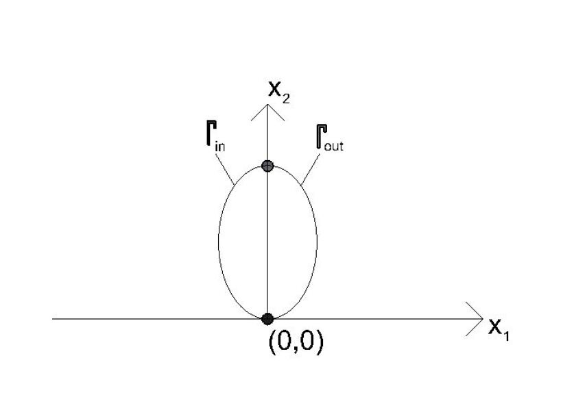
Figure 1: The domain. Simple representative case with two singularity points.

We assume further that these are the only singularity points, that is, the are no singularity points ’inside’ $\Gamma_{in}$ and $\Gamma_{out}$. An example of such domain is shown in Figure 1. It is well known and was already mentioned in the introduction that existence of regular solutions to inflow problem (1) requires certain assumptions on the shape of the boundary around the singularity points. We also need an assumption of this kind, in order to formulate it notice that around each singularity point the boundary is given as a function $x_{2}(x_{1})$. We assume it satisfies the condition

$$\exists N\in\mathbb{N}:\;|x_{2}(x_{1})-x_{2}(y_{1})|\geq C|x_{1}-y_{1}|^{N}\quad\forall x_{1},y_{1}:\;(x_{1},x_{2}(x_{1})),(y_{1},x_{2}(y_{1}))\in\Gamma^{s}_{in}.$$ (16)

We emphasize that the above condition is required only on the inflow part, therefore it can be rewritten as

$$\exists\delta>0:\;|\underline{x_{1}}(x_{2})-\underline{x_{1}}(y_{2})|\leq C|x_{2}-y_{2}|^{\delta}\quad\textrm{with}\quad\delta=\frac{1}{N}.$$ (17)

Remark 1.

Notice that if (16) is satisfied by some $N^{*}$ then it is also satisfied for $N>N*$ for small $|x_{2}-y_{2}|$. This condition means that the boundary around a singularity point must be less flat than some polynomial. Moreover we shall emphasize that (16) is a necessary but not sufficient condition; we also require sufficient global regularity of the boundary in order to solve an auxilary elliptic problem. In order to avoid additional technicalities we assume that $\Omega$ is a $C^{3}$ domain. Such regularity is obviously not assured by (16), in particular a Lipschitz boundary may satisfy (16) for any $N\geq 1$.

Remark 2.

A similar domain is considered in [14] and it is worth to compare the condition (17) with a similar constraint there with $\delta\geq\frac{1}{2}$. Therefore our condition is clearly weaker and means that the boundary around the singularity points is less flat then some polynomial.

Another interesting observation concerning the condition (16) is that a polynomial behaviour of the boundary near the singularity points turns out important in a completely different context of singularity of boundary layers in the stationary Munk equation, see [6].

Although condition (17) seems quite technical in the above formulation, it is in fact satisfied by a wide class of functions, in particular by piecewise analytical boundaries what is shown in the following lemma:

Lemma 1.

Assume that $x_{2}$ is an analytic function of $x_{1}$ around the singularity points. Then (16) holds.

Proof. By (15) we have $x_{2}^{\prime}(x_{1})=0$ at the singularity points. Therefore it is enough to show that if $f:\mathbb{R}\to\mathbb{R}$ is analytic in some $[-r,r]$, $f(0)=f^{\prime}(0)=0$ and $f\neq 0$ then

$$|f(x)|\geq C|x|^{N}\quad\textrm{for}\quad x\in(-l,l)$$ (18)

for some $C>0$, $N\geq 2$ and $l<r$ sufficiently small. Since $f\neq 0$ and $f$ is analytic, we must have $f^{(n)}(0)\neq 0$ for some $n\geq 2$. Let $f^{(k)}(0)$ be the first derivative not vanishing in $0$. Then we have

$$f(x)=\frac{f^{(k)}(0)}{k!}x^{k}+R^{k+1}(x),$$

where $|R^{k+1}(x)|\leq M|x|^{k+1}$ for $x\in(-r,r)$. Hence

$$|f(x)|\geq\Big{|}\frac{f^{k}(0)}{k!}\Big{|}|x|^{k}-M|x|^{k+1}=\Big{(}\frac{f^{k}(0)}{k!}-M|x|\Big{)}|x|^{k}.$$

$\square$

1.4 The domain. General case

Our result holds for a wide class of domains where the inflow and outflow parts are defined in a natural way. A general setting is to consider inflow and outflow described as

$$\begin{array}[]{c}\Gamma_{in}=\{(\underline{x_{1}}(x_{2}),x_{2}):x_{2}\in(a,b)\},\\[5.0pt] \Gamma_{out}=\{(\overline{x_{1}}(x_{2}),x_{2}):x_{2}\in(a,b)\},\\ \end{array}$$ (19)

with singularity points given by $\{(\underline{x_{1}}(x_{2}),x_{2}),x_{2}=k_{in}^{i}\}$ and $\{(\overline{x_{1}}(x_{2}),x_{2}),x_{2}=k_{out}^{j}\}$ where

$${\rm lim}_{x_{2}\to k_{in}^{i-}}|\underline{x_{1}}^{\prime}(x_{2})|={\rm lim}_{x_{2}\to k_{in}^{i+}}|\underline{x_{1}}^{\prime}(x_{2})|=\infty,$$

$${\rm lim}_{x_{2}\to k_{out}^{j-}}|\overline{x_{1}}^{\prime}(x_{2})|={\rm lim}_{x_{2}\to k_{out}^{j+}}|\overline{x_{1}}^{\prime}(x_{2})|=\infty.$$

Furthermore we assume

$$\begin{array}[]{c}{\rm lim}_{x_{2}\to a^{+}}\underline{x_{1}}(x_{2})=c_{1},\quad{\rm lim}_{x_{2}\to b^{-}}\underline{x_{1}}(x_{2})=c_{2},\\[5.0pt] {\rm lim}_{x_{2}\to a^{+}}\overline{x_{1}}(x_{2})=d_{1},\quad{\rm lim}_{x_{2}\to b^{-}}\overline{x_{1}}(x_{2})=d_{2}\end{array}$$ (20)

with $c_{i}\leq d_{i}$. Then we have

$$\Gamma_{0}=(c_{1},d_{1})\times\{a\}\cup(c_{2},d_{2})\times\{b\}.$$ (21)

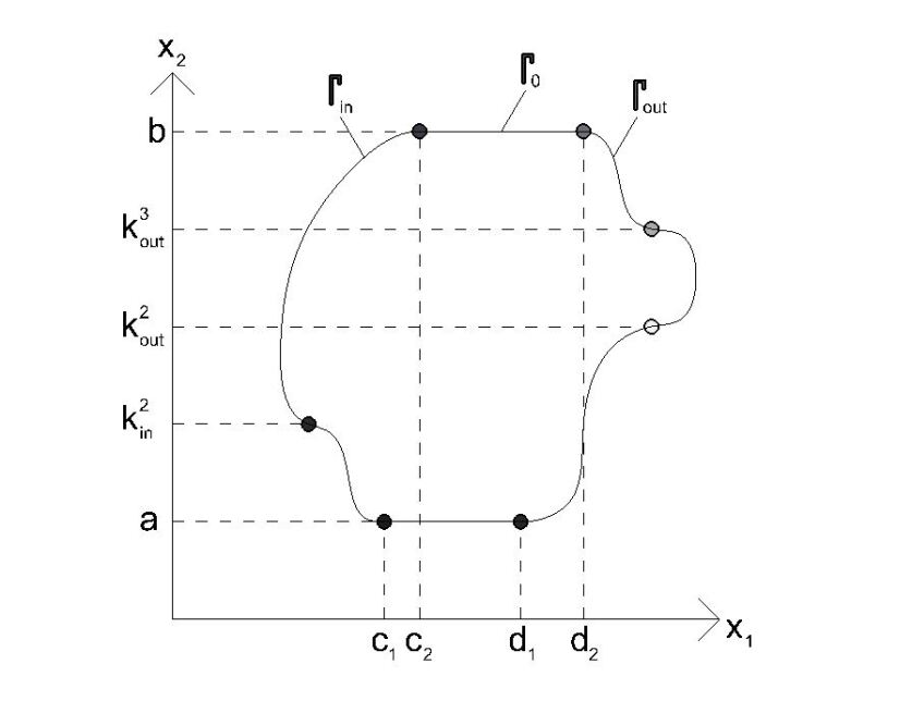
Figure 2: The domain. General case

An example of above described general domain is shown in Figure 2. Again, around singularity points $x_{2}$ is given as a function $x_{2}^{i}(x_{1})$ and we assume these functions to satisfy (16).

1.5 Main result

We are now in a position to formulate our main result.

Theorem 1.

Assume that $\Omega$ satifies the conditions introduced above, in particular (17). Assume the following regularity of the boundary data:

$$b\in W^{s-1/p}_{p}(\Gamma),\quad d\in W^{1+s-1/p}_{p}(\Gamma),$$ (22)

$$\rho_{in}\in W^{s}_{p}(\Gamma_{in})\cap W^{r}_{p}(\Gamma^{s}_{in}),$$ (23)

where

$$s<\delta,\quad r>\frac{s}{\delta}.$$ (24)

Let the pressure be in the form

$$\pi(\rho)=K\rho$$ (25)

for some positive constant $K$. Let the viscosity $\mu$ be sufficiently large compared to $|\Omega|$, $\|\bar{v}\|_{L_{\infty}}$ and $K$. Assume further that the boundary data satisfy following additional assumption:

$$|(d-n_{1})|\sqrt{1+|\underline{x_{1}}^{\prime}(x_{2})|^{2}}\leq\kappa<1,\qquad(A1)$$

Assume that $D_{0}$ defined in (12) is small enough and let $f$ be large enough on $\Gamma_{in}$. Then there exists a solution $(v,\rho)\in W^{1+s}_{p}\times W^{s}_{p}$ to the system (1) such that

$$\|v-\bar{v}\|_{W^{1+s}_{p}}+\|\rho-\bar{\rho}\|_{W^{s}_{p}}\leq E(D_{0}),$$ (26)

where $E(\cdot)$ is a Lipschitz function, E(0)=0. Moreover, this solution is unique in the class of solutions satisfying (26).

Remark 3.

Condition (23) is required to obtain the estimate for the density near the singularity points, the details are shown in the proofs of Lemmas 6 and 7. Therefore, for $\delta$ given by the geometry of the domain in (17) we can choose arbitrarily small $r$ provided we choose sufficiently small $s$, but we have to compensate it with sufficiently large $p$. Note that in particular we can assume

$$\rho_{in}\in W^{s}_{p}(\Gamma_{in})\cap W^{1}_{p}(\Gamma^{s}_{in}).$$ (27)

The rest of the paper is organized as follows. In the remaining of the present section we reformulate the problem (1) introducing perturbations as new unknowns, obtaining system (30). Then we recall basic properties of the functional spaces we use. In Section 2 we introduce linearization of (30) and show a priori estimates. First we show the energy estimate. Then in Section 2.2 we move to the estimate in $W^{s}_{p}$ for the steady transport equation which is the main difficulty in the proof. This result makes it possible to conclude the estimate in $W^{1+s}_{p}\times W^{s}_{p}$ in Sections 2.3 and 2.4. In Section 3 we prove Theorem with an interative scheme using our estimates for the linear system to show the convergence of the sequence of approximations. Finally we finish with a short concluding section. Without loss of generality we assume in the proofs $v^{*}=1$ in (11) except the proof of Proposition 3 where we need to track the dependence of the viscosity on this constant.

To remove inhomogeneity from the boundary condition (30)₄, we construct $u_{0}\in W^{1+s}_{p}$ such that

$$u_{0}\cdot n|_{\Gamma}=d-n_{1},\quad\|u_{0}\|_{W^{1+s}_{p}}\leq C\|d-n_{1}\|_{W^{1+s-1/p}_{p}(\Gamma)}.$$ (28)

For our purpose we find $u_{0}$ as a solution to the problem

$$-\mu\Delta u_{0}-(\mu+\nu)\nabla{\rm div}u_{0}=0,\quad u_{0}\cdot n=d-n_{1}.$$ (29)

In order to construct $u_{0}$ we supply (29) with condition $u_{0}\cdot\tau=0$ and define $u_{0}=u_{0}^{1}+u_{0}^{2}$, where $u_{0}^{1}\in W^{1+s}_{p}$ is any extension of the boundary data $d-n_{1}$ and $u_{0}^{2}$ solves

$$-\mu\Delta u_{0}^{2}-(\mu+\nu)\nabla{\rm div}u_{0}^{2}=\mu\Delta u_{0}^{1}+(\mu+\nu)\nabla{\rm div}u_{0}^{1},\quad u_{0}^{2}|_{\Gamma}=0.$$

Introducing the perturbations

$$u=v-\bar{v}-u_{0}\quad{\rm and}\quad w=\rho-\bar{\rho}$$

we obtain the system

$$\begin{array}[]{lcr}\partial_{x_{1}}u-\mu\Delta u-(\nu+\mu)\nabla{\rm div}\,u+K\,\nabla w=F(u,w)&\mbox{in}&\Omega,\\[3.0pt] {\rm div}\,u+\partial_{x_{1}}w+(u+u_{0})\cdot\nabla w=G(u,w)&\mbox{in}&\Omega,\\[3.0pt] n\cdot 2\mu{\bf D}(u)\cdot\tau+f\ u\cdot\tau=B&\mbox{on}&\Gamma,\\[3.0pt] n\cdot u=0&\mbox{on}&\Gamma,\\[3.0pt] w=w_{in}&\mbox{on}&\Gamma_{in},\end{array}$$ (30)

where

$$F(u,w) =-w\,(u+\bar{v}+u_{0})\cdot\nabla(u+u_{0})-\partial_{x_{1}}u_{0}-(u+u_{0})\cdot\nabla(u+u_{0}),$$

$$G(u,w) =-(w+1)\,{\rm div\,}u_{0}-w\,{\rm div\,}u,$$

$$B =b-f\tau^{(1)}-2\mu\,n\cdot\mathbf{D}(u_{0})\cdot\tau.$$ (31)

Notice that in general $F(u,w)$ contains a term $\mu\Delta u_{0}+(\nu+\mu)\nabla{\rm div}\,u_{0}$ which vanishes due to our definition of $u_{0}$. It can be seen easily that

$$\|F(u,w)\|_{L_{p}} \leq C[\|w\|_{W^{s}_{p}}\|u\|_{W^{1+s}_{p}}+E(\|\nabla u,u,w\|_{L_{p}}+1)],$$

$$\|G(u,w)\|_{W^{s}_{p}} \leq C[\|w\|_{W^{s}_{p}}\|u\|_{W^{1+s}_{p}}+E(\|w\|_{W^{s}_{p}}+1)],$$

$$\|B\|_{W^{s-1/p}_{p}} \leq C[\|b-f\tau\|_{W^{s-1/p}_{p}}+\|d-n_{1}\|_{W^{1+s-1/p}_{p}(\Gamma)}],$$ (32)

where $E$ is a small constant dependent on $\|u_{0}\|_{W^{1+s}_{p}}$ and $V^{*}$ is a dual space to $V$ defined in (9).

From now on we focus on the system (30). Our goal is to show the existence of a solution $(u,w)\in W^{1+s}_{p}\times W^{s}_{p}$ for given small function $u_{0}\in W^{1+s}_{p}$. Recall in particular that solution to the system (30) is used in the definition of solution to the the original problem (1). In order to define the solution to (30) we need its weak formulation. For this purpose we apply the identity

$$\int_{\Omega}(-\mu\Delta u-(\nu+\mu)\nabla\,{\rm div}u)\cdot v\,dx=\int_{\Omega}2\mu{\bf D}(u):\nabla\,v+\nu\,{\rm div}\,u\,{\rm div}\,v\,dx$$

$$-\int_{\Gamma}n\cdot[2\mu{\bf D}(u)]\cdot v\,d\sigma-\int_{\Gamma}n\cdot[\nu({\rm div}u){\bf{Id}}]\cdot v\,d\sigma.$$ (33)

Then a natural definition is following

Definition 2.

A regular $W^{s}_{p}$ solution to the problem (30) is a couple $(u,w)\in W^{1+s}_{p}\times W^{s}_{p}$ such that

$$\int_{\Omega}\psi\partial_{x_{1}}u\,dx+\int_{\Omega}(2\mu{\bf D}(u):\nabla\psi+\nu{\rm div\,}u{\rm div\,}\psi)\,dx+\int_{\Gamma}[f(u\cdot\tau)(\psi\cdot\tau)-b(\psi\cdot\tau)]\,d\sigma$$

$$-\int_{\Omega}w{\rm div\,}\psi\,dx=\int_{\Omega}F(u,w)\cdot\psi\,dx\quad\forall\psi\in V$$ (34)

and

$$\int_{\Omega}\phi{\rm div\,}u\,dx-\int_{\Omega}w((\bar{v}+u+u_{0})\cdot\nabla\phi+\phi{\rm div\,}(u+u_{0}))\,dx+\int_{\Gamma_{in}}w_{in}\phi\,d\sigma=$$

$$=\int_{\Omega}G(u,w)\phi\,dx\quad\forall\phi\in C^{1}(\Omega):\phi|_{\Gamma\setminus\Gamma_{in}}=0.$$ (35)

2 Linearization and a priori bounds

In this section we derive a priori estimates for the following linearization of system (30)

$$\begin{array}[]{lcr}\partial_{x_{1}}u-\mu\Delta u-(\nu+\mu)\nabla{\rm div}\,u+K\,\nabla w=F&\mbox{in}&\Omega,\\[3.0pt] {\rm div}\,u+\partial_{x_{1}}w+U\cdot\nabla w=G&\mbox{in}&\Omega,\\[3.0pt] n\cdot 2\mu{\bf D}(u)\cdot\tau+f\ u\cdot\tau=B&\mbox{on}&\Gamma,\\[3.0pt] n\cdot u=0&\mbox{on}&\Gamma,\\[3.0pt] w=w_{in}&\mbox{on}&\Gamma_{in},\\[3.0pt] \end{array}$$ (36)

where $U\in W^{1+s}_{p}$ is small and satisfies $U\cdot n|_{\Gamma}=d-n_{1}$ and on the rhs we have

$$F\in L_{p}(\Omega),\;G\in W^{s}_{p}(\Omega)\;\textrm{and}\;B\in W^{s-1/p}_{p}(\Gamma).$$ (37)

We start with the energy estimate, then we deal with the steady transport equation which is the main difficulty of our proof and finally we show the estimate in the solution space.

2.1 Energy estimate

In this section we show energy estimate for the solutions of (36).

Lemma 2.

Let $(u,w)$ be a sufficiently smooth solution to system (36) with given functions $(F,G,B)\in(V^{*}\times L_{2}\times L_{2}(\Gamma))$. Then

$$\|u\|_{W^{1}_{2}}+\|w\|_{L_{2}}\leq C\big{[}\|F\|_{V^{*}}+\|G\|_{L_{2}}+\|B\|_{L^{2}(\partial\Omega)}\big{]},$$ (38)

where $C$ is independent from the boundary data.

Proof. Multiplying the first equation of (36) by $u$ and integrating over $\Omega$ we get using the boundary condition (36)₃ and the identity (1.5):

$$\int_{\Omega}2\mu{\bf D}^{2}(u)+\nu{\rm div\,}^{2}udx+\int_{\partial\Omega}\left(f+\frac{n_{1}}{2}\right)u^{2}d\sigma+\int_{\Omega}K\nabla wudx=$$

$$-\int_{\Omega}u\,\partial_{x_{1}}u\,dx+\int_{\Omega}Fudx+\int_{\partial\Omega}B(u\cdot\tau)\,d\sigma.$$ (39)

The boundary term on the lhs will be positive for $f\geq 0$ on $\Gamma_{out}$ and $f\geq\frac{n_{1}}{2}$ on $\Gamma_{in}$. Next we integrate by parts the last term of the l.h.s of (2.1). Using (36)₂ we obtain:

$$K\int_{\Omega}u\nabla wdx =-K\int_{\Omega}w{\rm div\,}udx=K\int_{\Omega}(w\partial_{x_{1}}w+U\cdot w\nabla w-Gw)dx$$

$$=K\Big{[}\frac{1}{2}\int_{\Gamma}w^{2}n_{1}d\sigma-\frac{1}{2}\int_{\Omega}w^{2}{\rm div}\,U-\int Gwdx\Big{]}.$$ (40)

We will also use the following Korn inequality:

$$\int_{\Omega}2\mu{\bf D^{2}}(u)+\nu{\rm div\,}^{2}u\,dx\geq C_{K}\|u\|_{W_{2}^{1}(\Omega)}^{2},$$ (41)

where $C_{K}=C_{K}(\Omega)$. Using (2.1), (2.1) and (41) we get:

$$\|u\|_{W_{2}^{1}(\Omega)}^{2}+\int_{\Gamma_{out}}w^{2}n_{1}\,d\sigma\leq$$

$$\leq C\left[\int_{\Omega}w^{2}{\rm div}\,U\,dx+\gamma\int_{\Omega}Gw\,dx+\int_{\Omega}Fu\,dx+\int_{\Gamma}B(u\cdot\tau)\,d\sigma+\int_{\Gamma_{in}}w_{in}^{2}n_{1}d\sigma\right].$$

Next, using Hölder and Young inequalities, the fact that $w^{2}n_{1}>0$ on $\Gamma_{out}$ and the trace theorem to the boundary term we get for any $\delta>0$:

$$\begin{array}[]{c}\|u\|^{2}_{W^{1}_{2}(\Omega)}\leq\big{(}\delta+\|U\|_{W^{1+s}_{p}(\Omega)}\big{)}\|w\|_{L_{2}(\Omega)}^{2}+C(\delta)\|G\|_{L_{2}(\Omega)}^{2}+C\left[\big{(}\|F\|_{V^{*}}+\|B\|_{L_{2}(\Gamma)}\big{)}\|u\|_{W^{1}_{2}(\Omega)}\right],\end{array}$$

which yields

$$\begin{array}[]{c}\|u\|_{W^{1}_{2}(\Omega)}\leq\big{(}\delta+\|U\|_{W^{1+s}_{p}(\Omega)}\big{)}\|w\|_{L_{2}(\Omega)}+C(\delta)\|G\|_{L_{2}(\Omega)}+C(\|F\|_{V^{*}}+\|B\|_{L_{2}(\Gamma)}).\end{array}$$ (42)

To estimate the first term of the r.h.s. we find a bound on $\|w\|_{L_{2}}$. From $(\ref{system_lin})_{2}$ we have

$$\partial_{x_{1}}w+U\cdot\nabla w=G-{\rm div}\,u.$$

In order to estimate $\|w\|_{L_{2}}$, for $x\in\Omega$ let us denote by $\gamma_{x}$ a characteristic of the operator $\partial_{x_{1}}+U\cdot\nabla$ connecting $x$ with $\Gamma_{in}$, i.e. solution to

$$\left\{\begin{array}[]{c}\dot{\gamma_{x}}(t)=-(1-U_{1}(\gamma_{x}(t)),U_{2}(\gamma_{x}(t))),\\ \gamma_{x}(0)=x.\end{array}\right.$$ (43)

Notice that we take the tangential vector with opposite sign since we consider a backwards characteristic starting at a given point inside $\Omega$. Denote by $x^{in}(x)$ the intersection of $\gamma_{x}$ with $\Gamma_{in}$. Due to regularity and smallness of $U$, $\gamma_{x}$ is close to a straight line $\{x_{2}=c\}$. Now we can write

$$w(x)=w_{in}(x^{in}(x))+\int_{\gamma_{x}}(G-\rm{div}\,u)\,dl_{\gamma_{x}}.$$ (44)

By Jensen inequality we have

$$\left(\int_{\gamma}(G-\rm{div}\,u)dl_{\gamma_{x}}\right)^{2}\leq|\gamma_{x}|\int_{\gamma_{x}}|G|^{2}+|{\rm div}\,u|^{2}dl_{\gamma_{x}}.$$

Hence applying (44) we get

$$\|w\|_{L_{2}(\Omega)}\leq C(\Omega)\left(\|w_{in}\|_{L_{2}(\Gamma_{in})}+\|G\|_{L_{2}(\Omega)}+\|u\|_{W^{1}_{2}(\Omega)}\right).$$ (45)

Now we combine (42) and (45). By smallness of $U$ we can fix $\delta$ in (42) small enough to put the term $\delta+\|U\|_{W^{1+s}_{p}}$ on the left obtaining (38), which completes the proof of the lemma.

$\square$

2.2 Steady transport equation

In this section we show the estimate in $W^{s}_{p}$ for the steady transport equation with inflow condition which is a crucial step in showing a priori estimate for the linear problem (36).

Proposition 1.

Let $\Omega$ be a set defined at the end of Section 1, satisfying (17). Let $w$ solve

$$\bar{K}w+w_{x_{1}}+U\cdot\nabla w=H,\quad w|_{\Gamma_{in}}=w_{in},$$ (46)

where $\bar{K}$ is a positive constant, $U\in W^{1}_{\infty}(\Omega)$ is small and satisfies $U\cdot n|_{\Gamma}=d-n_{1}$ satisfying (A1). Assume $H\in W^{s}_{p}(\Omega)$ and let $w_{in}$, $s$ and $p$ satisfy the assumptions of Theorem 1. Then

$$\|w\|_{W^{s}_{p}(\Omega)}\leq C[\|H\|_{W^{s}_{p}(\Omega)}+\|w_{in}\|_{W^{s}_{p}(\Gamma_{in})\cap W^{r}_{p}(\Gamma_{s})}],$$ (47)

where $C=C(s,p,\Omega)$ and $r$ is from (24).

Remark 4.

Notice that the assumption $U\in W^{1}_{\infty}(\Omega)$ is weaker than $U\in W^{1+s}_{p}(\Omega)$ for $sp>2$ due to the imbedding theorem.

Remark 5.

Proposition 1 generalizes the result from [29] where it is assumed $U=[u^{1},0]$ which enables much simpler proof that the one presented below and no additional regularity of the density around the singularity points is required.

For simplicity we set $\bar{K}=1$ which is allowed as we assume anyway sufficient smallness of the data. The proof of Proposition 1 is quite technical since we have to treat carefully the boundary terms. For the reader’s convenience we divide it into several lemmas.

Lemma 3.

Let the assuptions of Proposition 1 hold. Then

$$\|w\|_{W^{s}_{p}(\Omega)}+\frac{1}{p}\iint_{\Omega^{2}}\frac{\partial_{x_{1}}|w(x)-w(y)|^{p}+\partial_{y_{1}}|w(x)-w(y)|^{p}}{\phi_{\epsilon}(x,y)}dxdy\\ +\frac{1}{p}\iint_{\Omega^{2}}\frac{U(x)\cdot\nabla_{x}|w(x)-w(y)|^{p}+U(y)\cdot\nabla_{y}|w(x)-w(y)|^{p}}{\phi_{\epsilon}(x,y)}dxdy\leq\|H\|_{W^{s}_{p}(\Omega)}\|w\|_{W^{s}_{p}}^{p-1}.$$ (48)

Proof. Recalling the definition of Sobolev-Slobodetskii norm we write (46) in $x$ and $y$. Using identities of a kind of $\nabla_{x}w(y)=0$ we can write

$$w(x)+\partial_{x_{1}}[w(x)-w(y)]+U(x)\cdot\nabla_{x}[w(x)-w(y)]=H(x),$$

$$w(y)+\partial_{y_{1}}[w(y)-w(x)]+U(y)\cdot\nabla_{y}[w(y)-w(x)]=H(y).$$

We multiply the first equation by $\frac{|w(x)-w(y)|^{p-2}(w(x)-w(y))}{\phi_{\epsilon}(x,y)}$ and the second by
$\frac{|w(x)-w(y)|^{p-2}(w(y)-w(x))}{\phi_{\epsilon}(x,y)}$, where

$$\phi_{\epsilon}(x,y)=\epsilon+|x-y|^{2+sp}.$$

Then we add the equations and integrate twice over $\Omega$, w.r.t. $x$ and $y$. Since

$$w(x)(w(x)-w(y))+w(y)(w(y)-w(x))=[w(x)-w(y)]^{2}$$

and

$$H(x)(w(x)-w(y))+H(y)(w(y)-w(x))=(H(x)-H(y))(w(x)-w(y)),$$

we obtain on the left hand side

$$\iint_{\Omega^{2}}\frac{|w(x)-w(y)|^{p}}{\phi_{\epsilon}(x,y)}\,dxdy\to_{\epsilon\to 0}\|w\|_{W^{s}_{p}}^{p}.$$ (49)

On the r.h.s we have using Hölder inequality:

$$\iint_{\Omega^{2}}\frac{(H(x)-H(y))|w(x)-w(y)|^{p-2}(w(x)-w(y))}{\phi_{\epsilon}(x,y)}\leq$$

$$\Big{(}\iint_{\Omega^{2}}\frac{|H(x)-H(y)|^{p}}{\phi_{\epsilon}(x,y)}\Big{)}^{1/p}\Big{(}\iint_{\Omega^{2}}\frac{|w(x)-w(y)|^{p}}{\phi_{\epsilon}(x,y)}\Big{)}^{1-1/p}\to_{\epsilon\to 0}\|H\|_{W^{s}_{p}}\|w\|_{W^{s}_{p}}^{p-1},$$ (50)

which completes the proof of (48).

$\square$

The rest of the proof of Proposition 1 consist in dealing with the integral terms in (48). This is where all the difficulties are hidden and our assumptions on the boundary and boundary data will come into play. We start with observing that under the assumptions of Proposition 1 we have

$$n_{1}+U\cdot n\geq 0\quad{\rm on}\quad\Gamma_{out}.$$ (51)

Indeed, we have

$$n(x)|_{\Gamma_{out}}=\frac{[1,-\overline{x_{1}}^{\prime}(x_{2})]}{\sqrt{1+[\overline{x_{1}}^{\prime}(x_{2})]^{2}}},\qquad n(x)|_{\Gamma_{in}}=\frac{[-1,\underline{x_{1}}^{\prime}(x_{2})]}{\sqrt{1+[\underline{x_{1}}^{\prime}(x_{2})]^{2}}},$$ (52)

therefore by (A1)

$$\left|\frac{U\cdot n}{n_{1}}\right|=\sqrt{1+[\overline{x_{1}}^{\prime}(x_{2})]^{2}}|U\cdot n|\leq\kappa,$$

and so (51) holds.

We now proceed with transforming (48). Since we want to have a $W^{s}_{p}$ norm, we have to get rid of the derivatives of $w$ and for this purpose we integrate by parts. This step is presented in the following lemma

Lemma 4.

Let the assumptions of Proposition 1 be satisfied. Then

$$\|w\|_{W^{s}_{p}(\Omega)}^{p}+\frac{2}{p}\int_{\Omega}\int_{\Gamma_{in}}\frac{|w(x)-w(y)|^{p}(n_{1}+U\cdot n)(x)}{\phi_{\epsilon}}dS(x)dy\leq$$

$$\leq\|H\|_{W^{s}_{p}(\Omega)}\|w\|_{W^{s}_{p}(\Omega)}^{p-1}+C\|\nabla U\|_{L_{\infty}(\Omega)}\|w\|_{W^{s}_{p}(\Omega)}^{p}.$$ (53)

Proof. We will obtain (4) from (48). Let us start with the first integral term on the lhs of (48). We have

$$\frac{\partial_{x_{1}}|w(x)-w(y)|^{p}}{\phi_{\epsilon}(x,y)}=\partial_{x_{1}}\Big{(}\frac{|w(x)-w(y)|^{p}}{\phi_{\epsilon}(x,y)}\Big{)}-|w(x)-w(y)|^{p}\partial_{x_{1}}\Big{(}\frac{1}{\phi_{\epsilon}(x,y)}\Big{)}.$$ (54)

By the definition of $\phi_{\epsilon}(x,y)$ we have

$$\nabla_{x}\phi_{\epsilon}(x,y)=-\nabla_{y}\phi_{\epsilon}(x,y),$$ (55)

therefore using (54) we get

$$\iint_{\Omega^{2}}\Big{\{}\frac{\partial_{x_{1}}|w(x)-w(y)|^{p}}{\phi_{\epsilon}(x,y)}+\frac{\partial_{y_{1}}|w(y)-w(x)|^{p}}{\phi_{\epsilon}(x,y)}\Big{\}}\,dxdy=$$

$$=\iint_{\Omega^{2}}\Big{\{}\partial_{x_{1}}\Big{(}\frac{|w(x)-w(y)|^{p}}{\phi_{\epsilon}(x,y)}\Big{)}+\partial_{y_{1}}\Big{(}\frac{|w(x)-w(y)|^{p}}{\phi_{\epsilon}(x,y)}\Big{)}\Big{\}}\,dxdy$$

$$-\iint_{\Omega^{2}}\Big{\{}|w(x)-w(y)|^{p}\partial_{x_{1}}\Big{(}\frac{1}{\phi_{\epsilon}(x,y)}\Big{)}+|w(x)-w(y)|^{p}\partial_{y_{1}}\Big{(}\frac{1}{\phi_{\epsilon}(x,y)}\Big{)}\Big{\}}\,dxdy.$$ (56)

Taking into account (55), the integrand in the second integral on the rhs of (2.2) vanishes identically. Combining (55) with the identities

$$\nabla_{x}|w(x)-w(y)|^{p}=p|w(x)-w(y)|^{p-2}(w(x)-w(y))\nabla_{x}w(x)$$ (57)

and

$$\nabla_{y}|w(x)-w(y)|^{p}=-p|w(x)-w(y)|^{p-2}(w(x)-w(y))\nabla_{y}w(y),$$ (58)

we see that the first integral on the rhs of (2.2) adds up to

$$\frac{2}{p}\iint_{\Omega^{2}}\partial_{x_{1}}\Big{(}\frac{|w(x)-w(y)|^{p}}{\phi_{\epsilon}(x,y)}\Big{)}\,dxdy=\frac{2}{p}\int_{\Omega}\int_{\Gamma}\frac{|w(x)-w(y)|^{p}n_{1}}{\phi_{\epsilon}(x,y)}\,dS(x)\,dy.$$ (59)

Now consider the second integral on the lhs of (48). We have

$$\iint_{\Omega^{2}}U(x)\frac{\nabla_{x}|w(x)-w(y)|^{p}}{\phi_{\epsilon}(x,y)}\,dxdy=$$

$$=\iint_{\Omega^{2}}U(x)\nabla_{x}\Big{(}\frac{|w(x)-w(y)|^{p}}{\phi_{\epsilon}(x,y)}\Big{)}\,dxdy-\iint_{\Omega^{2}}U(x)|w(x)-w(y)|^{p}\nabla_{x}\Big{(}\frac{1}{\phi_{\epsilon}(x,y)}\Big{)}\,dxdy$$ (60)

and

$$\iint_{\Omega^{2}}U(y)\frac{\nabla_{y}|w(x)-w(y)|^{p}}{\phi_{\epsilon}(x,y)}\,dxdy=$$

$$=\iint_{\Omega^{2}}U(y)\nabla_{y}\Big{(}\frac{|w(x)-w(y)|^{p}}{\phi_{\epsilon}(x,y)}\Big{)}\,dxdy-\iint_{\Omega^{2}}U(y)|w(x)-w(y)|^{p}\nabla_{y}\Big{(}\frac{1}{\phi_{\epsilon}(x,y)}\Big{)}\,dxdy.$$ (61)

Recalling (55) we see that the terms with $\nabla\big{(}\frac{1}{\phi}\big{)}$ cancel. But this time the integrand does not vanish identically and we have to check whether the sum of these integrals makes sense when $\epsilon\to 0$. This sum equals

$$\left|\iint_{\Omega^{2}}[U(x)-U(y)]|w(x)-w(y)|^{p}\frac{(2+sp)|x-y|^{sp}(x-y)}{(\epsilon+|x-y|^{2+sp})^{2}}\,dxdy\right|\longrightarrow_{\epsilon\to 0}$$

$$(2+sp)\left|\iint_{\Omega^{2}}\frac{U(x)-U(y)}{x-y}\frac{|w(x)-w(y)|^{p}}{|x-y|^{2+sp}}\,dxdy\right|\leq C\|\nabla U\|_{L_{\infty}}\|w\|_{W^{s}_{p}}^{p}.$$

Now consider the terms with $\nabla\frac{|w(x)-w(y)|^{p}}{\phi_{\epsilon}}$ on the r.h.s. of (2.2) and (2.2). Combining (57) and (58) with (55) we see that these terms add up to

$$\frac{2}{p}\iint_{\Omega^{2}}U(x)\nabla_{x}\Big{(}\frac{|w(x)-w(y)|^{p}}{\phi_{\epsilon}(x,y)}\Big{)}\,dxdy=$$

$$=-\int_{\Omega}dy\int_{\Omega}\frac{|w(x)-w(y)|^{p}}{\phi_{\epsilon}(x,y)}{\rm div}_{x}U(x)\,dx+\int_{\Omega}dy\int_{\Gamma}\frac{|w(x)-w(y)|^{p}}{\phi_{\epsilon}(x,y)}U(x)\cdot n\,dS(x).$$ (62)

The first integral is straighforward:

$$\Big{|}\int_{\Omega}dy\int_{\Omega}\frac{|w(x)-w(y)|^{p}}{\phi_{\epsilon}(x,y)}{\rm div}_{x}U(x)\,dx\Big{|}\leq C(\Omega)\|\nabla U\|_{L_{\infty}(\Omega)}\|w\|_{W^{s}_{p}(\Omega)}^{p}.$$ (63)

Combining (48), (59), (2.2) and (63) we get (4).

$\square$

In order to complete the proof of Proposition 1 it remains to find an estimate on the integral term in (4). Notice that it is sufficient to consider the integral over $\Gamma_{in}$ since the outflow part is nonnegative due to (51) and therefore we already skipped it in (4). However, the inflow term is negative because of $n_{1}$ and therefore must be estimated. The treatment of this term is quite technical and in fact constitutes the core of the proof of Proposition 1. Let us start with introducing some further notation. In the estimate which will follow, $y=(y_{1},y_{2})$ will denote a point inside $\Omega$ while $\underline{x}=(\underline{x}_{1},\underline{x}_{2})$ a point on $\Gamma_{in}$. In several places we will replace an integral with respect to the boundary measure on $\Gamma_{in}$ by an integral w.r.t $x_{2}$. Then we will write $\underline{x}(x_{2})=(\underline{x_{1}}(x_{2}),x_{2})$. At this point we should also fix $\eta$ in the definition (10). For this purpose observe that (A1) implies

$$|(d-n_{1})|\sqrt{1+|\underline{x_{1}}^{\prime}(x_{2})|^{2}}\leq\frac{\tilde{\kappa}}{\sqrt{1+\lambda^{2}}}$$ (64)

for some $\kappa<\tilde{\kappa}<1$ and $\lambda>0$. Now in (10) we choose $\eta$ such that

$$|x_{2}^{\prime}(x_{1})|<\lambda\quad{\rm on}\;\Gamma^{s}_{in}.$$ (65)

Notice that such $\eta$ exists due to assumed regularity of the boundary. Next we define

$$\Gamma_{in}^{r}:=\{x\in\Gamma_{in}:\;\eta<x_{2}<b-\eta\},$$

$$\Omega_{in}^{r}:=\{x\in\Omega:\;\eta<x_{2}<b-\eta,\quad x_{1}-\underline{x_{1}}(x_{2})<\eta\},$$

$$\Omega_{in}^{s}:=\{x\in\Omega:\;x_{2}<2\eta\;\vee\;b-2\eta<x<b\},$$

$$\Omega_{in}=\Omega_{in}^{r}\cup\Omega_{in}^{s},$$ (66)

Therefore, $\Gamma_{in}^{r}$ and $\Omega_{in}^{r}$ are, respectively, a part of $\Gamma_{in}$ and its neighbourhood which are at some fixed distance from singularity points. In particular, we have

$$|\underline{x_{1}}^{\prime}(x_{2})|\leq C(\eta)\quad{\rm for}\quad(\underline{x_{1}}(x_{2}),x_{2})\in\Gamma_{in}^{r}.$$ (67)

Notice also that $\Gamma^{s}_{in}=\Omega^{s}_{in}\cap\Gamma_{in}$. Next, for $y=(y_{1},y_{2})$ let us denote by $\gamma_{y}$ a characteristic curve of the operator $(\partial_{x_{1}}+U\cdot\nabla)$ connecting $y$ with $\Gamma_{in}$, i.e. solution to (43) with $\gamma_{y}(0)=y$. Furthermore, we denote the intersection of $\gamma_{y}$ with $\Gamma_{in}$ by $y^{in}(y)$ (see Figure 3). We will need the following auxiliary result

Lemma 5.

Assume that

$$y\in\Omega_{in}^{r},\quad\underline{x}\in\Gamma_{in}^{r}.$$ (68)

Then

$$|\underline{x}-y^{in}(y)|+|y^{in}(y)-y|\leq C|\underline{x}-y|,$$ (69)

$$|\gamma_{y}|\leq(1+E)|y_{1}-\underline{x_{1}}(y_{2})|.$$ (70)

for some constant $C>0$ and a small constant $E$.

Proof. W.l.o.g. we can restrict to assuming that $x_{2}$ is a decreasing function of $x_{1}$ on $\Gamma_{in}$ as the opposite case is analogous. Then it is convenient to distiguish $3$ cases:

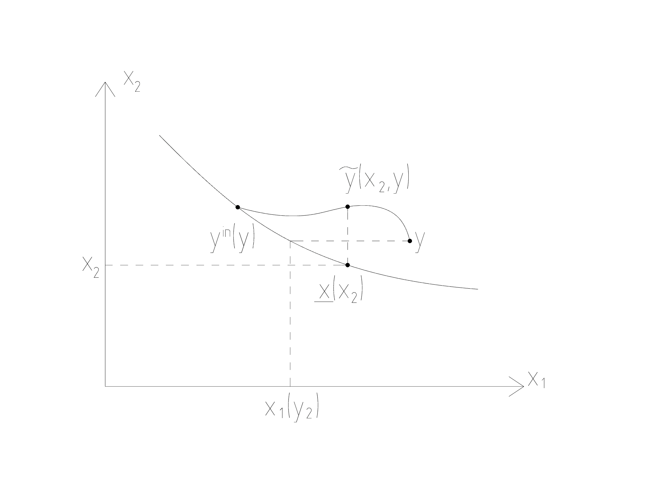
Figure 4: Illustration of notation. Case (b): intersection point $\tilde{y}$ well defined.

$$\textrm{{\bf(a)}}\quad\underline{x}_{1}\leq y^{in}_{1}(y)\;\textrm{(see Figure 4)};$$

$$\textrm{{\bf(b)}}\quad y^{in}_{1}(y)<\underline{x}_{1}<y_{1}\;\textrm{(see Figure 3)};$$ (71)

$$\textrm{{\bf(c)}}\quad\underline{x}_{1}\geq y_{1};$$

In the case (a) (69) is obvious with $C=2$ as $|\underline{x}-y^{in}(y)|\leq|\underline{x}-y|$ and $|y^{in}(y)-y|\leq|\underline{x}-y|$. The case (c) is treated similarly to (b), therefore we don’t show it on a separate figure and focus on the proof for (b). In that case it is convenient to define by $\tilde{y}(x_{2},y)$ the intersection of a line $\{(\underline{x_{1}}(x_{2}),t):t\in\mathbb{R}\}$ with a characteristic $\gamma_{y}$ connecting $\Gamma_{in}$ with $y$. Such intersection is well defined in the case b), see Figure 3. We have for some $\vartheta\in[\underline{x}_{2},y_{2}]$

$$|\underline{x}-y^{in}(y)|\leq C(|\underline{x}_{1}-y^{in}_{1}(y)|+|\underline{x}_{2}-y^{in}_{2}(y)|)=(C\underline{x_{1}}^{\prime}(\vartheta)+1)|\underline{x}_{2}-y^{in}_{2}(y)|$$

$$\leq C|\underline{x}_{2}-\tilde{y}_{2}(x_{2},y)|\leq C|\underline{x}-\tilde{y}(x_{2},y)|\leq C|\underline{x}-y|,$$ (72)

where we have used (67). Therefore also

$$|y^{in}(y)-y|\leq|y^{in}(y)-\underline{x}|+|\underline{x}-y|\leq C|\underline{x}-y|,$$

which completes the proof of the first assertion. To show the second one we can assume w.l.o.g. that $y^{in}_{2}(y)\geq y_{2}$. We have

$$|y^{in}_{2}(y)-y_{2}|=\int_{y^{in}_{1}(y)}^{y_{1}}U_{2}(t,\gamma(t))dt\leq\|U\|_{\infty}|y^{in}_{1}(y)-y_{1}|,$$

therefore using again (67) we get

$$|y_{1}-y^{in}_{1}(y)|\leq|y_{1}-\underline{x_{1}}(y_{2})|+|\underline{x_{1}}(y_{2})-y^{in}_{1}(y)|+|y^{in}_{2}(y)-y_{2}|\leq|y_{1}-\underline{x_{1}}(y_{2})|+(|\underline{x_{1}}^{\prime}(\theta)|+1)|y^{in}_{2}(y)-y_{2}|$$

$$\leq|y_{1}-\underline{x_{1}}(y_{2})|+(|\underline{x_{1}}^{\prime}(\theta)|+1)\|U_{2}\|_{\infty}|y_{1}-y^{in}_{1}(y)|,$$

so for sufficiently small $\|U\|_{\infty}$ we obtain

$$|y_{1}-y^{in}_{1}(y)|\leq(1+E)|y_{1}-\underline{x_{1}}(y_{2})|,$$

and to complete the proof it is enough to note that

$$|\gamma_{y}|=\int_{y^{in}_{1}(y)}^{y_{1}}\sqrt{[1+U_{1}(\gamma_{y}(s))]^{2}+(U_{2}(\gamma_{y}(s)))^{2}}ds\leq(1+E)|y_{1}-y^{in}_{1}(y)|.$$

$\square$

We shall emphasize that (69) holds except a neighborhood of singularity points. The point is that $|\underline{x_{1}}^{\prime}(x_{2})|$ is unbounded as we approach the singularity. Therefore, as

$$|\underline{x}(x_{2})-y^{in}(y_{2})|\geq|\underline{x_{1}}(x_{2})-y^{in}_{1}(y_{2})|=|\underline{x_{1}}^{\prime}(\vartheta)||x_{2}-y_{2}|$$ (73)

for some $\vartheta\in[x_{2},y_{2}]$, we no longer have (69). In order to control $|\underline{x}-y^{in}(y)|$ we need appropriate estimate on a length of a characteristic connecting $y$ with the boundary and here the assumptions (16) and (A1) come into play. The required result is

Lemma 6.

Let $b(t)=(t,\underline{x_{2}}(-t))$ and let $p(t)$ satisfy

$$\dot{p}(t)=(1+U^{1}(p(t)),U^{2}(p(t))),\quad p(t_{0})=x_{2}^{0}.$$ (74)

where $x_{2}^{0}$ is a given, small positive number, $t_{0}$ is sufficiently small that

$$p(s)>b(s)\quad{\rm for}\quad s\leq t_{0}.$$

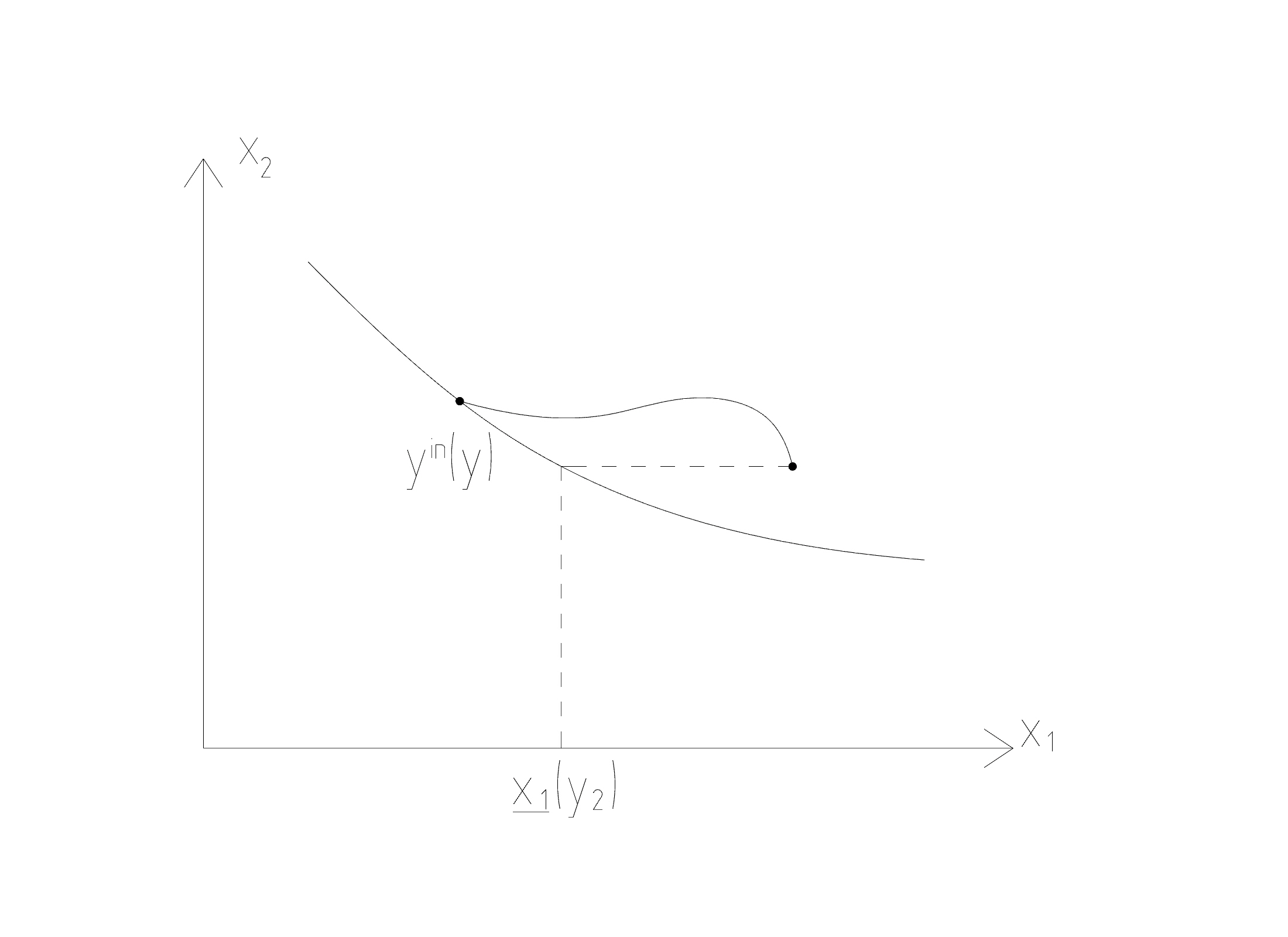
Figure 5: Case (a): no intersection point $\tilde{y}$.

and $U$ satisfies the assumptions of Proposition 1. Let $t_{*}$ denote the first coordinate of the first intersection of $p(t)$ and $b(t)$ (see Fig. 5). Then

$$t_{*}-t_{0}\leq C(x_{2}^{0}-b(t_{0}))^{\delta},$$

where $\delta$ is from (17) and $C=C(U,\Omega)$.

Remark 6.

We will apply the above lemma with $t=-x_{1}$ in some neighbourhood of a singularity point $(0,0)$ in the proof of Lemma 7 which will follow, therefore we consider a ’backward’ characteristic of the equation (46).

Proof. Assume first that $t_{0}=0$. Let us denote

$$A(t)=\sqrt{1+|\underline{x_{2}}^{\prime}(t)|^{2}}.$$

Then the unit normal to $b(t)$ is $n_{b}(t)={A(t)}^{-1}(-\underline{x_{2}}^{\prime}(t),1).$ Let $z(t)$ denote the distance between $b(t)$ and $p(t)$ measured along $n_{b}(t)$ (see Fig. 5), that is

$$p(t)=b(t)+n_{b}(t)z(t).$$

Differentiating this identity in $t$ and multiplying the resulting equation by $n_{b}(t)$ we get

$$\dot{p}(t)\cdot n_{b}(t)=\dot{z}(t),$$ (75)

Which by (74) rewrites

$$\dot{z}(t)=U\cdot n_{b}(t,z)-\frac{\underline{x_{2}}^{\prime}(t)}{A(t)}.$$ (76)

We have

$$|U\cdot n_{b}(t,z)|\leq|U\cdot n_{b}(t,0)|+\|\nabla U\|_{L_{\infty}}z,$$

therefore by (76)

$$\dot{z}(t)\leq|U\cdot n_{b}(t,0)|-\frac{\underline{x_{2}}^{\prime}(t)}{A(t)}+\|\nabla U\|_{L_{\infty}}z(t).$$ (77)

Now, due to (64) and (65) we have

$$|U\cdot n_{b}(t,0)|\leq\frac{\tilde{\kappa}|\underline{x_{2}}^{\prime}(t)|}{\sqrt{1+\lambda^{2}}}<\tilde{\kappa}\frac{|\underline{x_{2}}^{\prime}(t)|}{A(t)}$$ (78)

therefore

$$\dot{z}(t)\leq-(1-\tilde{\kappa})\frac{\underline{x_{2}}^{\prime}(t)}{A(t)}+E_{U}z(t)\leq-\theta+E_{U}z(t)$$ (79)

with $\theta=\frac{1-\tilde{\kappa}}{\sqrt{1+\lambda^{2}}}$ and $E_{U}=\|\nabla U\|_{L_{\infty}}$. Now $t_{*}$ must satisfy

$$\int_{0}^{t^{*}}\dot{z}(t)dt=-x_{2}^{0},\mbox{ \ therefore \ }x_{2}^{0}=\theta\underline{x_{2}}(t_{*})-E_{U}\underbrace{\int_{0}^{t_{*}}z(t)dt}_{Z(t_{*})}.$$ (80)

In order to simplify the above condition observe that

$$z(t)\leq x_{2}^{0}e^{E_{U}t}\leq Cx_{2}^{0},\quad p(t)-b(t)\leq Cz(t)$$

, and therefore

$$Z(t_{*})\leq t\,\sup_{s\leq t}[p(t)-b(t)]\leq C_{2}t_{*}x_{2}^{0}.$$ (81)

Moreover, by (16) we have

$$\underline{x_{2}}(t_{*})\geq C_{1}t_{*}^{N}.$$ (82)

In view of (81) and (82), if we define $\tilde{t}_{*}$ by

$$P_{x_{2}^{0}}(\tilde{t}_{*}):=C_{1}\theta\tilde{t}_{*}^{N}-C_{2}E_{U}x_{2}^{0}\tilde{t}_{*}-x_{2}^{0}=0,$$

then, because of (80),(81) and (82),

$$t_{*}\leq\tilde{t}_{*}$$

We claim that there exists $1\leq C_{3}=C_{3}(C_{1},C_{2},\Omega)$ s.t. if $t_{1}=C_{3}(x_{2}^{0})^{1/N}$ then $P(t_{1})\geq 0.$ Indeed, we have

$$P(t_{1})=x_{2}^{0}[C_{1}\theta C_{3}-1-C_{2}E_{U}(C_{3}x_{2}^{0})^{1/N}]\geq C_{3}(C_{1}-C_{2}E_{U}(x_{2}^{0})^{1/N})-1>0$$

for sufficiently large $C_{3}=C_{3}(C_{1},C_{2},\Omega)$. Therefore,

$$\tilde{t}_{*}\leq t_{1}\leq C_{3}(x_{2}^{0})^{1/N},$$

which together with (2.2) completes the proof for $t_{0}=0$ as $\delta=\frac{1}{N}$. For $t_{0}>0$ the reasoning is the same modulo minor adjustments, replacing $x_{2}^{0}$ with $-z(t_{0})$ in (80).

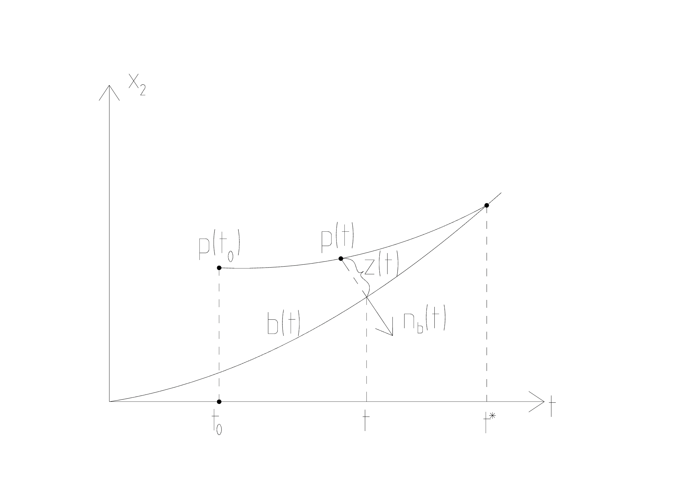
Figure 3: Explanation of notation used in Lemma 6

We are now in a position to prove the estimate on the boundary term on the lhs of (4).

Lemma 7.

Let the assuptions of Proposition 1 hold. Then

$$\int_{\Omega}dy\int_{\Gamma_{in}}\frac{|w(x)-w(y)|^{p}(n_{1}+U\cdot n)(x)}{\phi_{\epsilon}(x,y)}dS(x)\leq$$

$$\leq C[\|H\|_{L_{\infty}(\Omega)}+\|w\|_{L_{p}(\Omega)}+\|w\|_{L_{\infty}(\Omega)}+\|w_{in}\|_{W^{s}_{p}(\Gamma_{in})}+\|w_{in}\|_{W^{r}_{p}(\Gamma^{s}_{in})})]^{p}.$$ (83)

Proof. First of all, due to (52) and (A1) we have

$$|\frac{U\cdot n}{n_{1}}|\leq\kappa,$$

which gives

$$|n_{1}+U\cdot n|\leq(1+\kappa)n_{1}.$$ (84)

Therefore it is enough to show (7) for $U\cdot n=0$. As

$$dS(x_{2})|_{\Gamma_{out}}=\sqrt{1+[\overline{x_{1}}^{\prime}(x_{2})]^{2}}dx_{2}\quad\textrm{and}\quad dS(x_{2})|_{\Gamma_{in}}=\sqrt{1+[\underline{x_{1}}^{\prime}(x_{2})]^{2}}dx_{2},$$ (85)

(52) yields

$$dS(x_{2})|_{\Gamma_{in}}=-\frac{dx_{2}}{n_{1}},\qquad n_{2}dS(x_{2})|_{\Gamma_{in}}=\underline{x_{1}}^{\prime}(x_{2})dx_{2}.$$ (86)

By (86), assuming $U\cdot n=0$ the LHS of (7) can be rewritten as

$$\int_{\Omega}\int_{\Gamma_{in}}\frac{|w(x)-w(y)|^{p}n_{1}(x)}{\phi_{\epsilon}(x,y)}dS(x)dy=\int_{\Omega}dy\underbrace{\int_{0}^{b}-\frac{|w(\underline{x_{1}}(x_{2}),x_{2})-w(y)|^{p}}{\phi_{\epsilon}((\underline{x_{1}}(x_{2}),x_{2}),y)}\,dx_{2}}_{I_{\epsilon}(y)},$$ (87)

and it remains to show the estimate (7) for (87). When we pass with $\epsilon\to 0$, we can expect some problems only when $y$ is close to $\Gamma_{in}$. Therefore we write (87) as

$$\int_{\Omega}I_{\epsilon}(y)dy=\int_{\Omega^{r}_{in}}I_{\epsilon}(y)dy+\int_{\Omega^{s}_{in}}I_{\epsilon}(y)dy+\int_{\Omega\setminus\Omega_{in}}I_{\epsilon}(y)dy=:I_{1}^{r}+I_{1}^{s}+I_{2},$$

where the sets $\Omega^{r}_{in}$, $\Omega^{s}_{in}$ and $\Omega_{in}$ are defined in (2.2). The set $\Omega\setminus\Omega_{in}$ consist of points at the distance from $\Gamma_{in}$ bounded from below by $\eta$. Therefore the $I_{2}$ integral is straightforward as we have $|(\underline{x_{1}}(x_{2}),x_{2})-y|>\eta$ for $y\in\Omega\setminus\Omega_{in}$ and so

$$I_{2}\leq C(\eta)[\|w_{in}\|_{L_{p}(\Gamma_{in})}+\|w\|_{L_{p}}]^{p}.$$ (88)

The estimates for $I^{r}_{2}$ and $I^{s}_{1}$ are more involved, we show them in details.
Estimate of $I^{r}_{1}$. Let $\underline{x}(x_{2})=(\underline{x_{1}}(x_{2}),x_{2})\in\Gamma_{in}$. We have

$$\frac{|w(\underline{x}(x_{2}))-w(y)|^{p}}{|\underline{x}(x_{2})-y|^{2+sp}}\leq C(p)\left[\frac{|w(\underline{x}(x_{2}))-w(y^{in}(y))|^{p}}{|\underline{x}(x_{2})-y|^{2+sp}}+\frac{|w(y^{in}(y))-w(y)|^{p}}{|\underline{x}(x_{2})-y|^{2+sp}}\right].$$ (89)

For the first term on the rhs of (89) we have

$$\int_{\Omega^{r}_{in}}dy\int_{0}^{b}\frac{|w(\underline{x}(x_{2}))-w(y^{in}(y))|^{p}}{|\underline{x}(x_{2})-y|^{2+sp}}\,dx_{2}=$$

$$=\int_{2\eta}^{b-2\eta}dx_{2}\left[\int_{V_{\eta}(x_{2})}\frac{|w(\underline{x}(x_{2}))-w(y^{in}(y))|^{p}}{|\underline{x}(x_{2})-y|^{2+sp}}\,dy+\int_{\Omega^{r}_{in}\setminus V_{\eta}(x_{2})}\frac{|w(\underline{x}(x_{2}))-w(y^{in}(y))|^{p}}{|\underline{x}(x_{2})-y|^{2+sp}}\,dy\right],$$ (90)

where

$$V_{\eta}(x_{2})=\{y\in\Omega^{r}_{in}:\;x_{2}-\eta<y_{2}<x_{2}+\eta\},$$ (91)

which implies that in the second integral $|\underline{x}(x_{2})-y|$ is bounded from below by $\eta$, therefore

$$\int_{0}^{b}dx_{2}\int_{\Omega^{r}_{in}\setminus V_{\eta}(x_{2})}\frac{|w(\underline{x}(x_{2}))-w(y^{in}(y))|^{p}}{|\underline{x}(x_{2})-y|^{2+sp}}\,dy$$

$$\leq C\left[\int_{0}^{b}|w(\underline{x}(x_{2}))|^{p}dx_{2}+\int_{0}^{b}|w(y^{in}(y))|^{p}dy_{2}\right]\leq C\|w_{in}\|_{L_{p}(\Gamma_{in})},$$

where in the last passage we have used an obvious inequality

$$dy_{2}\leq dS(y_{2}).$$ (92)

In order to treat the first integral in (2.2) we apply (69)-(70). Due to (70) we can assume w.l.o.g. for this estimate that $\gamma_{y}$ is a straight line $y_{2}\equiv{\rm const}$, therefore $y^{in}(y)=\underline{y}(y)$. Then by the definitions of $V_{\eta}(x_{2})$ and $\Omega^{r}_{in}$ ((91) and (2.2), respectively)

$$\int_{V_{\eta}(x_{2})}\frac{|w(\underline{x}(x_{2}))-w(y^{in}(y))|^{p}}{|\underline{x}(x_{2})-y|^{2+sp}}\,dy=\int_{x_{2}-\eta}^{x_{2}+\eta}\int_{\underline{y_{1}}(y_{2})}^{\underline{y_{1}}(y_{2})+\eta}\frac{|w(\underline{x}(x_{2}))-w(y^{in}(y_{2}))|^{p}}{|\underline{x}(x_{2})-y|^{2+sp}}dy_{1}dy_{2}$$

$$\leq\int_{x_{2}-\eta}^{x_{2}+\eta}|w(\underline{x}(x_{2}))-w(y^{in}(y_{2}))|^{p}dy_{2}\int_{\underline{y_{1}}(y_{2})}^{\underline{y_{1}}(y_{2})+\eta}(y_{1}-\underline{y_{1}}(y)+|\underline{x}(x_{2})-y^{in}(y_{2})|)^{-2-sp}dy_{1}$$

$$\leq\int_{x_{2}-\eta}^{x_{2}+\eta}\frac{|w(\underline{x}(x_{2}))-w(y^{in}(y_{2}))|^{p}}{|\underline{x}(x_{2})-y^{in}(y_{2})|^{1+sp}}dy_{2},$$

where in the first inequality we have used (69). Therefore, as we have additionally (92),

$$\int_{2\eta}^{b-2\eta}dx_{2}\int_{V_{\eta}(x_{2})}\frac{|w(\underline{x}(x_{2}))-w(y^{in}(y))|^{p}}{|\underline{x}(x_{2})-y|^{2+sp}}\,dy\leq C\|w\|_{W^{s}_{p}(\Gamma_{in})}.$$ (93)

Notice that in this part of the estimate the norm of boundary data appears naturally.

In the second term on the r.h.s. of (89) we express $w(y)-w(y^{in}(y))$ by an integral along $\gamma_{y}$ using the equation (46). Applying Jensen inequality we get

$$\int_{\Omega^{r}_{in}}dy\int_{0}^{b}\frac{|w(y^{in}(y))-w(y)|^{p}}{|\underline{x}(x_{2})-y|^{2+sp}}\,dx_{2}\leq\int_{\Omega_{in}^{r}}dy\int_{0}^{b}\frac{|\int_{\gamma_{y}}(H-w)dl_{\gamma_{y}}|^{p}}{|\underline{x}(x_{2})-y|^{2+sp}}\,dx_{2}\leq$$

$$\leq(\|H\|_{L_{\infty}}+\|w\|_{L_{\infty}})^{p}\int_{\Omega_{in}^{r}}dy\int_{0}^{b}\frac{|\gamma_{y}|^{p}}{|\underline{x}(x_{2})-y|^{2+sp}}\,dx_{2}\leq$$

$$\leq C(\|H\|_{L_{\infty}}+\|w\|_{L_{\infty}})^{p}\int_{\Omega_{in}^{r}}dy\int_{0}^{b}\frac{|y^{in}(y)-y|^{p}}{|\underline{x}(x_{2})-y|^{2+sp}}\,dx_{2}\leq$$

$$\leq C(\|H\|_{L_{\infty}}+\|w\|_{L_{\infty}})^{p}\int_{0}^{b}dx_{2}\int_{\Omega_{in}^{r}}\frac{|\underline{x}(x_{2})-y|^{p}}{|\underline{x}(x_{2})-y|^{2+sp}}\,dy,$$ (94)

where we have used (69) and (70). The last integral is finite for $s<1$, we remember $\Omega^{r}_{in}$ is two dimensional. Combining (89), (93) and (2.2) we get

$$I_{1}^{r}\leq C(\|H\|_{L_{\infty}(\Omega)}+\|w\|_{L_{\infty}(\Omega)}+\|w_{in}\|_{W^{s}_{p}(\Gamma_{in})})^{p}.$$ (95)

Estimate of $I^{s}_{1}$. Around the singularity points we have to proceed more carefully. If we consider again separately the cases (2.2), then in the case (a) (69) still holds with $C=2$ so we can repeat directly the previous approach and it remains to consider the cases (b) and (c). The key difference is that, as we already explained, $|\underline{x_{1}}^{\prime}(x_{2})|$ is unbounded.

Therefore we cannot repeat directly (93) and (2.2). We have to control $|\underline{x}-y^{in}(y)|$ and here we use the assumption (17). Recall the notions of $\gamma_{y}$ and $\tilde{y}$ introduced in (43) and after (2.2), respectively, see Fig. 3. Let us denote by $\gamma_{\tilde{y}}$ the part of the $\gamma_{y}$ connecting $\Gamma_{in}$ with $\tilde{y}(x_{2},y)$. We modify (89) adding the point $\tilde{y}(x_{2},y)$:

$$\frac{|w(\underline{x}(x_{2}))-w(y)|^{p}}{|\underline{x}(x_{2})-y|^{2+sp}}\leq C(p)\left[\frac{|w(\underline{x}(x_{2}))-w(y^{in}(y))|^{p}}{|\underline{x}(x_{2})-y|^{2+sp}}+\frac{|w(y^{in}(y))-w(\tilde{y}(x_{2},y))|^{p}}{|\underline{x}(x_{2})-y|^{2+sp}}\right.$$

$$\left.+\frac{|w(\tilde{y}(x_{2},y))-w(y)|^{p}}{|\underline{x}(x_{2})-y|^{2+sp}}\right].$$ (96)

We start with the 2nd and 3rd term on the rhs of (2.2). Similarly as before, in both terms we replace the value of $w$ with an integral along $\gamma_{y}$. The last term is analogous to $I_{1}^{r}$ and we get

$$\int_{\Omega^{s}_{in}}\,dy\int_{0}^{b}\frac{|w(\tilde{y}(x_{2},y))-w(y)|^{p}}{|\underline{x}(x_{2})-y|^{2+sp}}\,dx_{2}\leq C(\|H\|_{L_{\infty}(\Omega)}+\|w\|_{L_{\infty}(\Omega)})^{p}\quad\textrm{for}\quad s<1.$$ (97)

In the second term we have

$$|w(\tilde{y}(x_{2},y))-w(y^{in}(y))| =|\int_{\gamma_{\tilde{y}}}(H-w)dl_{\gamma_{\tilde{y}}}|$$

$$\leq(\|H\|_{L_{\infty}}+\|w\|_{L_{\infty}})\int_{y^{in}_{1}(y)}^{\underline{x_{1}}(x_{2})}\sqrt{[1+U_{1}(\gamma_{y}(s))]^{2}+(U_{2}(\gamma_{y}(s)))^{2}}{\rm ds}$$

$$\leq C(\|H\|_{L_{\infty}}+\|w\|_{L_{\infty}})|y^{in}_{1}(y)-\underline{x_{1}}(x_{2})|.$$

Now we estimate the latter term. This is the most subtle part of the whole proof which has been carried out in Lemma 6. Applying this result with $t_{0}=-\underline{x_{1}}(x_{2})$ we have

$$|y^{in}_{1}(y)-\underline{x_{1}}(x_{2})|\leq C|x_{2}-\tilde{y}_{2}(x_{2},y)|^{\delta},$$ (98)

where $\delta$ is from (17). Next,

$$|x_{2}-\tilde{y}_{2}(x_{2},y)|\leq|x_{2}-y_{2}|+\|U_{2}\|_{L_{\infty}(\Omega)}|x_{1}-y_{1}|\leq C|\underline{x}-y|,$$

therefore

$$\int_{\Omega^{s}_{in}}dy\int_{0}^{b}\frac{|w(y^{in}(y))-w(\tilde{y}(x_{2},y))|^{p}}{|\underline{x}(x_{2})-y|^{2+sp}}\leq\int_{\Omega^{s}_{in}}dy\int_{0}^{b}\frac{|\int_{\gamma_{\tilde{y}}}(H-w)dl_{\gamma_{\tilde{y}}}|^{p}}{|\underline{x}(x_{2})-y|^{2+sp}}\,dx_{2}\leq$$

$$\leq C(\|H\|_{L_{\infty}}+\|w\|_{L_{\infty}})^{p}\int_{\Omega^{s}_{in}}dy\int_{0}^{b}\frac{|x_{2}-\tilde{y}_{2}(x_{2},y)|^{\delta p}}{|\underline{x}(x_{2})-y|^{2+sp}}\,dx_{2}\leq$$

$$\leq C(\|H\|_{L_{\infty}}+\|w\|_{L_{\infty}})^{p}\int_{\Omega^{s}_{in}}dy\int_{0}^{b}|\underline{x}(x_{2})-y|^{\delta p-2-sp}\,dx_{2},$$

where in the second passage we used (98). The last integral is finite for $s<\delta$ and we conclude

$$\int_{\Omega^{s}_{in}}\,dy\int_{0}^{b}\frac{|w(y^{in}(y))-w(\tilde{y}(x_{2},y))|^{p}}{|\underline{x}(x_{2})-y|^{2+sp}}\,dx_{2}\leq C(\|H\|_{L_{\infty}}+\|w\|_{L_{\infty}})^{p}\quad\textrm{for}\quad s<\delta.$$ (99)

It remains to estimate the first term on the rhs of (2.2). For this purpose we assume $\underline{x}\neq y^{in}(y)$ since otherwise this term vanishes. By Fubini’s theorem we have $dy=dS(y_{2})dy_{1}$, therefore we can write

$$\int_{\Omega^{s}_{in}}dy\int_{0}^{b}\frac{|w(\underline{x}(x_{2}))-w(y^{in}(y))|^{p}}{|\underline{x}(x_{2})-y|^{2+sp}}dx_{2}$$

$$\leq C\int_{\Gamma^{s}_{in}}dS(y_{2})\int_{0}^{b}dx_{2}\int_{\underline{y_{1}}(y_{2})}^{\overline{y_{1}}(y_{2})}\frac{|w(\underline{x}(x_{2}))-w(\underline{y}(y_{2})))|^{p}}{[|\underline{x_{1}}(x_{2})-y_{1}|+|x_{2}-y_{2}|]^{2+sp}}dy_{1}$$

$$\leq C\int_{\Gamma^{s}_{in}}dS(y_{2})\int_{0}^{b}dx_{2}\frac{|w(\underline{x}(x_{2}))-w(\underline{y}(y_{2}))|^{p}}{|x_{2}-y_{2}|^{1+sp}}.$$ (100)

Introducing $h=x_{2}-y_{2}$ and using the imbedding (8) we get

$$\int_{\Gamma^{s}_{in}}dS(y_{2})\int_{0}^{b}dx_{2}\frac{|w(\underline{x}(x_{2}))-w(\underline{y}(y_{2}))|^{p}}{|x_{2}-y_{2}|^{1+sp}}$$

$$\leq C\int_{0}^{h_{0}}\frac{dh}{|h|^{1+sp}}\int_{\Gamma^{s,h}_{in}|w(\underline{x}(y_{2}+h))-w(\underline{y}(y_{2}))|^{p}dS(y_{2})}$$ (101)

$$\leq C\|w\|_{B^{r}_{p,\infty}(\Gamma^{s}_{in})}\int_{0}^{h_{0}}h^{-1-sp}{\rm sup}_{y_{2}\in(0,\eta)}|\underline{x}(y_{2}+h)-\underline{y}(y_{2})|^{rp}dh$$

$$\leq C\|w\|_{W^{r}_{p}(\Gamma^{s}_{in})}\int_{0}^{h_{0}}h^{-1-sp}{\rm sup}_{y_{2}\in(0,\eta)}|\underline{x}(y_{2}+h)-\underline{y}(y_{2})|^{rp}dh,$$

where

$$h_{0}={\rm sup}\{x_{2}:\;(\underline{x_{1}}(x_{2}),x_{2})\in\Gamma^{s}_{in}\}\quad{\rm and}\quad{\Gamma^{s,h}_{in}}=\{\underline{x}(x_{2}):\;\underline{x}(x_{2}+h)\in\Gamma^{s}_{in}\}.$$

In the second passage in (2.2) we have used (7) and in the last one (8). Now we apply Lemma 6 with

$$t_{0}=-x_{1},\quad p(t_{0})=(y^{in}_{1}(y_{2}),y_{2}+h),\quad p(t)=\gamma_{p(t_{0})}(-t),$$

where $\gamma_{y}(\cdot)$ is a characteristic passing through $y$ defined in (43). Then Lemma 6 implies

$$|\underline{x}(y_{2}+h)-\underline{y}(y_{2})|\leq C|\underline{x}(y_{2}+h)-p(t_{0})|\leq C|h|^{\delta},$$ (102)

which together with (2.2) gives

$$\int_{\Gamma^{s}_{in}}dS(y_{2})\int_{0}^{b}dx_{2}\frac{|w(\underline{x}(x_{2}))-w(\underline{y}(y_{2}))|^{p}}{|x_{2}-y_{2}|^{1+sp}}\leq C\|w\|_{W^{r}_{p}(\Gamma^{s}_{in})}\int_{0}^{h_{0}}h^{\delta rp-1-sp}.$$ (103)

The last integral is finite provided

$$\delta r>s$$

, which implies the second relation in (24). Combining (97), (99) and (103) we conclude

$$I^{s}_{1}\leq C(\|H\|_{L_{\infty}}+\|w\|_{L_{\infty}}+\|w_{in}\|_{W^{r}_{p}(\Gamma_{s})})^{p}.$$ (104)

Putting together (88),(95) and (104) we get (7) with $U\cdot n=0$, which completes the proof due to (84).

$\square$

Proof of Proposition 1. Now we are ready to close the estimate (47). Combining (4) with (7) we obtain

$$\|w\|_{W^{s}_{p}}^{p}\leq C(s,p,\Omega)[\|H\|_{W^{s}_{p}}\|w\|_{W^{s}_{p}}^{p-1}+\|w\|_{L_{\infty}}^{p}+\|w\|_{L_{p}}^{p}$$

$$+\|w_{in}\|_{W^{s}_{p}(\Gamma_{in})}+\|w_{in}\|_{W^{r}_{p}(\Gamma_{s})}+\|\nabla U\|_{L_{\infty}}\|w\|_{W^{s}_{p}}^{p}]$$ (105)

and applying the interpolation inequality (6) we conclude (47).

$\square$

Remark 7.

Notice that from (2.2) it follows that the constant in (47) is of a form $C=\frac{C(s,p,\Omega)}{1-\|\nabla U\|_{L_{\infty}}}$, therefore under the assumption of smallness of $\|\nabla U\|_{L_{\infty}}$ we can assume that it does not depend on $\|\nabla U\|_{L_{\infty}}$.

Remark 8.

The proof of Proposition 1 is quite technical, therefore it may be unclear for the reader how it can be extended to more general domain. To clarify it, we shall emphasize that the most subtle part is the estimate of $\frac{|w(\underline{x})-w(y)|^{p}}{|\underline{x}-y|^{2+sp}}$ where $\underline{x}$ is on the boundary and $y$ is inside $\Omega$, both close to singularity. The most delicate point is to estimate the distance between the point where a characteristic crossing $y$ intersects the boundary and $\underline{x}$. This was carried out in Lemma 6. On the other hand, larger distance between $\underline{x}$ and $y$ does not entail additional problems. Therefore the proof presented here can be extended to the general case of multiple singularity points. We have to consider again separately the ’regular’ part of the boundary where $\underline{x_{2}}^{\prime}(x_{1})$ is bounded by a given constant and therefore we get the estimates (88), (95), and neighbourhoods of each singularity point where we repeat the estimate (104).

$\square$

2.3 Linear estimate in $W^{1+s}_{p}\times W^{s}_{p}$ and solution of the linear system

In this section we solve linear problem (36) with rhs of regularity determined in (37). First we show the a priori estimate.

Proposition 2.

Let $(u,w)$ solve the system (36) with the rhs of regularity determined in (37) with $s,p$ and the boundary data satisfying the assumptions of Theorem 1. Then we have

$$\|u\|_{W^{1+s}_{p}(\Omega)}+\|w\|_{W^{s}_{p}(\Omega)}\leq\\ C\,[\|F\|_{L_{p}(\Omega)}+\|G\|_{W^{s}_{p}(\Omega)}+\|w_{in}\|_{W^{s}_{p}(\Gamma_{in})\cap W^{r}_{p}(\Gamma_{s})}+\|B\|_{W^{1-1/p}_{p}(\Gamma)}].$$ (106)

Remark 9.

The main difficulty in the proof of (106) lies in the steady transport equation which has been dealt with in Proposition 1. The rest of the proof uses classical results from the theory of elliptic problems and can be divided in several steps.

Proof of Proposition 2. Step I. Let us take the rotation of $(\ref{system_lin})_{1}$. Then we get the following system

$$\begin{array}[]{lcr}-\mu\Delta{\rm rot\,}u={\rm rot\,}(F-\partial_{x_{1}}u)&\mbox{in}&\Omega,\\[3.0pt] {\rm rot\,}u=(2\chi-f/\nu)u\cdot\tau+\frac{B}{\mu}&\mbox{ at }\Gamma.\end{array}$$ (107)

In order to show the boundary relation for the vorticity we differentiate (36)₃ in the tangential direction and apply (36)₄. The details are shown in [21] in the case $u\cdot n=d,\;B=0$. A minor modification for our case $u\cdot n=0,B\neq 0$ yields (107). We find the following estimate for the solution to (107):

$$\|{\rm rot\,}u\|_{W^{1}_{p}(\Omega)}\leq C(\|F\|_{L_{p}(\Omega)}+\|u,B\|_{W^{1-1/p}_{p}(\Gamma)}+\|\partial_{x_{1}}u\|_{L_{p}(\Omega)}).$$ (108)

The solvability of (107) belongs to the classical theory of elliptic linear problems, hence we omit the details of this construction.

Step II. Consider the Helmholtz decomposition of $u$:

$$u=\nabla\phi+\nabla^{\bot}A.$$ (109)

We have $0=n\cdot\nabla^{\bot}A=\tau\cdot\nabla A$. Therefore $A$ satifies

$$\Delta A={\rm rot\,}u,\quad A|_{\Gamma}={\rm const}.$$ (110)

As $\partial\Omega\in C^{3}$, from (110) we obtain

$$\|A\|_{W^{3}_{p}(\Omega)}\leq C\|{\rm rot\,}u\|_{W^{1}_{p}(\Omega)}.$$ (111)

Substituting (109) to $(\ref{system_lin})_{1}$ we get

$$\nabla(-(2\mu+\nu){\rm div\,}u+Kw)=F-\partial_{x_{1}}u+\mu\Delta\nabla^{\bot}A+(\mu+\nu)\nabla{\rm div\,}\nabla^{\bot}A=:\bar{F}.$$

By (108) and (111) we have

$$\|\bar{F}\|_{L_{p}(\Omega)}\leq C[\|F\|_{L_{p}(\Omega)}+\|\partial_{x_{1}}u\|_{L_{p}(\Omega)}+\|u,B\|_{W^{1-1/p}_{p}(\Gamma)}],$$

therefore denoting

$$-(2\mu+\nu){\rm div\,}u+Kw=H$$ (112)

we have for any $\delta>0$

$$\|H\|_{W^{s}_{p}(\Omega)}\leq \delta\|\nabla H\|_{L_{p}(\Omega)}+C(\delta)\|H\|_{L_{2}(\Omega)}\leq\delta[\|F\|_{L_{p}(\Omega)}+\|\partial_{x_{1}}u\|_{L_{p}(\Omega)}+\|u,B\|_{W^{1-1/p}_{p}(\Gamma)}]$$

$$+C(\delta)\|\nabla u,w\|_{L_{2}(\Omega)}.$$ (113)

Step III. Adding $(\ref{system_lin})_{2}$ to (112) with suitable scaling we obtain

$$\partial_{x_{1}}w+U\cdot\nabla w+\bar{K}w=\bar{G}$$ (114)

with $\bar{K}=\frac{K}{2\mu+\nu}$ and

$$\|\bar{G}\|_{W^{s}_{p}(\Omega)}\leq\|G\|_{W^{s}_{p}(\Omega)}+[RHS\;of\;\eqref{AP5}].$$

Here we meet the main mathematical challange of our result, we have to solve this transport like problem in a domain which touches the characteristics at the ends of $\Gamma_{in}$. Its solvability is given by Proposition 1. In particular, the estimate (47) yields

$$\|w\|_{W^{s}_{p}(\Omega)}\leq C(\|G\|_{W^{s}_{p}(\Omega)}+\|w_{in}\|_{W^{s}_{p}(\Gamma_{in})\cap W^{r}_{p}(\Gamma_{s})}).$$ (115)

Remark 10.

Notice that Remark 7 implies that we can assume that the constant in (115) does not depend on $\|U\|_{W^{1}_{\infty}}$.

Step IV. We collect the elements of our estimation. In order to get the information about the velocity we use estimates for ${\rm rot\,}u$ given by (108) and about ${\rm div\,}u$ coming from (112),(2.3) and (115). We obtain

$$\|u\|_{W^{1+s}_{p}(\Omega)}\leq C(\|{\rm rot\,}u\|_{W^{s}_{p}(\Omega)}+\|{\rm div\,}u\|_{W^{s}_{p}(\Omega)})$$

$$\leq C(\|F\|_{L_{p}(\Omega)}+\|G\|_{W^{s}_{p}(\Omega)}+\|B\|_{W^{1-1/p}(\Gamma)}+\|\nabla u,w\|_{L_{2}(\Omega)} +\|\partial_{x_{1}}u\|_{L_{p}}+\|u\|_{W^{1-1/p}(\Gamma)})$$

$$+\delta(\|u\|_{W^{1+s}_{p}(\Omega)}+\|w\|_{W^{s}_{p}(\Omega)}).$$ (116)

The $L_{2}$ term on the rhs is treated with the energy estimate (38). To the boundary term $\|u\|_{W^{1-1/p}(\Gamma)}$ we apply first trace theorem and then interpolation inequality (6) to get

$$\|u\|_{W^{1-1/p}_{p}(\Gamma)}\leq C\|u\|_{W^{s}_{p}(\Omega)}\leq\delta\|u\|_{W^{1+s}_{p}(\Omega)}+C(\delta)\|\nabla u\|_{L_{2}(\Omega)}.$$ (117)

The term $\partial_{x_{1}}u$ is treated similarly with interpolation inequality. We conclude (106) and complete the proof.

$\square$

Now it is a matter of standard theory to show the existence for the linear system (36).

Proposition 3.

Let the rhs of (36) be of regularity specified in (37) with $s,p$ and the boundary data satisfying the assumptions of Theorem 1. Then there exists a unique solution to (36) satisfying the estimate (106).

Proof. As we have the a priori estimate, the proof of existence is standard. We start with showing the weak solutions using the Galerkin method and the energy estimate (38). Then, using our a priori estimate we show that our solution has the required regularity.

$\square$

2.4 Estimate for the nonlinear system

We are now ready to close the estimate in $W^{1+s}_{p}\times W^{s}_{p}$ for the nonlinear system. To this end we combine the linear estimate (106) with the bounds (1.5) on the rhs of the nonlinear problem obtaining

$$\|u\|_{W^{1+s}_{p}(\Omega)}+\|w\|_{W^{s}_{p}(\Omega)}\leq E(\|u\|_{W^{1+s}_{p}(\Omega)}+\|w\|_{W^{s}_{p}(\Omega)}+1)+C(\|u\|_{W^{1+s}_{p}(\Omega)}+\|w\|_{W^{s}_{p}(\Omega)})^{2},$$

where $E$ is a small constant dependent on the data and we can assume (see Remark 10) that $C$ does not depend on $\|u\|_{W^{1}_{\infty}(\Omega)}$. For sufficiently small data we conclude

$$\|u\|_{W^{1+s}_{p}(\Omega)}+\|w\|_{W^{s}_{p}(\Omega)}\leq C(\|u\|_{W^{1+s}_{p}(\Omega)}+\|w\|_{W^{s}_{p}(\Omega)}^{2}+E,$$ (118)

where $C$ does not depend on $(\|w\|_{W^{s}_{p}(\Omega)},\|u\|_{W^{1+s}_{p}(\Omega)})$. This estimate will be crucial in showing the existence and uniqueness of solutions in the next section.

Remark 11.

Notice that the estimate (118) holds without any assumptions on relation between $\mu$ and $K$. However, this relation will come into play in the following section.

3 Proof of Theorem 1

In order to prove our main result we apply an iterative scheme. The idea is to combine the estimate (118) with the Cauchy condition in some weaker space. In [27],[30] this space was $H^{1}\times L_{2}$. However, then we need some information on the gradient of the density which is not available in our framework. Here we overcome this obstacle showing the convergence in $L_{2}\times H^{-1}$. However, then we have to estimate $\|\pi(\rho^{n})-\pi(\rho^{n-1})\|_{H^{-1}}$ in terms of $\|\rho^{n}-\rho^{n-1}\|_{H^{-1}}$ and for this purpose we have to assume (25). A similar approach was applied in the context of uniqueness of weak solutions in the nonstationary case in [12] where the constraint (25) also appeared. Under this assumption, denoting

$$v^{n+1}=u^{n+1}+u_{0}+\bar{v}$$

we can define the sequence of approximations in the following way

$$\begin{array}[]{lcr}{\rm div\,}(w^{n+1}v^{n+1}\otimes v^{n+1})-\mu\Delta u^{n+1}-(\mu+\nu)\nabla{\rm div\,}u^{n+1}+K\nabla w^{n+1}=0&\mbox{in}&\Omega,\\[3.0pt] w^{n+1}_{x_{1}}+{\rm div\,}((u^{n}+u_{0})w^{n+1})=-{\rm div\,}(u^{n}+u_{0})&\mbox{in}&\Omega,\\[3.0pt] n\cdot 2\mu{\bf D}(u^{n+1})\cdot\tau+fu^{n+1}\cdot\tau=B&\mbox{on}&\Gamma,\\[3.0pt] n\cdot u^{n+1}=0&\mbox{on}&\Gamma,\\[3.0pt] w^{n+1}=w_{in}&\mbox{on}&\Gamma_{in}.\end{array}$$ (119)

We start with the following auxiliary result

Lemma 8.

Assume that $\phi$ solves

$$(\partial_{x_{1}}+U\cdot\nabla)\phi=f,\quad\phi|_{\Gamma_{out}}=0$$ (120)

with $f\in H^{1}_{0}(\Omega)$ and sufficiently small $U\in W^{1}_{\infty}(\Omega)$ such that

$$U\cdot n|_{\Gamma_{in}}<0,\quad U\cdot n|_{\Gamma_{out}}>0.$$ (121)

Then

$$\|\nabla\phi\|_{L_{2}(\Omega)}\leq C_{\Omega}\|f\|_{H^{1}_{0}(\Omega)}$$ (122)

where $C_{\Omega}\sim{\rm max}\{|\Omega|,|\Omega|^{2}\}$.

Proof. The boundary condition (120)₂ implies

$$0=\partial_{\tau}\phi|_{\Gamma_{out}}=\tau_{1}\phi_{x_{1}}+\tau_{2}\phi_{x_{2}}|_{\Gamma_{out}}.$$ (123)

On the other hand we have

$$(1+u^{1})\phi_{x_{1}}+u^{2}\phi_{x_{2}}|_{\Gamma_{out}}=0.$$ (124)

Subtracting (123) multiplied by $u^{2}$ from (124) multiplied by $\tau^{2}$ w get

$$0=[(1+u^{1})\tau^{2}-u^{2}\tau^{1})]\phi_{x_{1}}=-[(1+u^{1})n^{1}+u^{2}n^{2}]\phi_{x_{1}}=0,$$

therefore $\phi_{x_{1}}|_{\Gamma_{out}}=0$ due to (121). Combining this identity with (123) we conclude

$$\nabla\phi|_{\Gamma_{out}}=0.$$ (125)

Next we differentiate (120)₁ wrt $x_{2}$ and multiply by $\phi_{x_{2}}$. Denoting $V=[1+U^{1},U^{2}]$ we obtain

$$\frac{1}{2}V\cdot\nabla\phi_{x_{2}}^{2}=f_{x_{2}}\phi_{x_{2}}-V_{x_{2}}\phi_{x_{2}}\cdot\nabla\phi.$$ (126)

Now let us denote

$$\Omega_{a}=\Omega\cap\{x_{1}>a\},\quad I_{a}=\Omega\cap\{x_{1}=a\}.$$

Integrating (126) over $\Omega_{a}$ we get

$$\frac{1}{2}\int_{\partial\Omega_{x_{1}}}(V\cdot n)\phi_{x_{2}}^{2}\,d\sigma=\int_{\Omega_{x_{1}}}\Big{[}\frac{1}{2}\phi_{x_{2}}^{2}{\rm div\,}V+f_{x_{2}}\phi_{x_{2}}+V_{x_{2}}\phi_{x_{2}}\cdot\nabla\phi\Big{]}\,dx.$$ (127)

Notice that by (125) and the condition $V\cdot n|_{\Gamma_{in}}<0$ we have

$$\int_{\partial\Omega\,\cap\,\partial\Omega_{x_{1}}}(V\cdot n)\phi_{x_{2}}^{2}\,d\sigma\leq 0.$$

Therefore the smallness of $U^{1}$ implies

$$\int_{\partial\Omega_{x_{1}}}(V\cdot n)\phi_{x_{2}}^{2}\,d\sigma=-\int_{I_{x_{1}}}(1+U^{1})\phi_{x_{2}}^{2}\,dx_{2}+\int_{\partial\Omega\,\cap\,\partial\Omega_{x_{1}}}(V\cdot n)\phi_{x_{2}}^{2}\,d\sigma\leq-C_{U}\int_{I_{x_{1}}}\phi_{x_{2}}^{2}\,d\sigma$$

for some $C_{U}>0$. The latter inequality combined with (127) gives for any $\epsilon>0$

$${\rm sup}_{x_{1}}\int_{I_{x_{1}}}\phi_{x_{2}}^{2}\,dx_{2}\leq\|\nabla U\|_{L_{\infty}(\Omega)}\|\nabla\phi\|_{L_{\infty}(\Omega)}+\epsilon\|\phi_{x_{2}}\|_{L_{2}(\Omega)}^{2}+\frac{C}{\epsilon}\|\nabla f\|_{L_{2}(\Omega)}^{2}.$$

Using again smallness of $U$ we obtain

$$\|\phi_{x_{2}}\|_{L_{2}(\Omega)}^{2}\leq|\Omega|[(\epsilon+\|\nabla U\|_{L_{\infty}(\Omega)})\|\nabla\phi\|_{L_{2}(\Omega)}^{2}+C(\epsilon)\|\nabla f\|_{L_{2}(\Omega)}^{2}].$$ (128)

Finally from (120)₁ we have

$$\|\phi_{x_{1}}\|_{L_{2}(\Omega)}^{2}\leq\|\frac{f}{1+U^{1}}\|_{L_{2}(\Omega)}^{2}+\|\frac{U^{2}}{1+U^{1}}\|_{L_{\infty}(\Omega)}\|\phi_{x_{2}}\|_{L_{2}(\Omega)}^{2}.$$

Combining this inequality with (128) we get

$$\|\nabla\phi\|_{L_{2}(\Omega)}^{2}\leq[|\Omega|(\epsilon+\nabla U\|_{L_{\infty}(\Omega)})+C\|U\|_{L_{\infty}(\Omega)}]\|\nabla\phi\|_{L_{2}(\Omega)}^{2}+[\frac{C|\Omega|}{\epsilon}+C_{p}]\|\nabla f\|_{L_{2}(\Omega)}^{2}$$

where $C_{p}$ is the constant from the Poincaré inequality. Now, provided $\|U\|_{W^{1}_{\infty}}$ is sufficiently small, to close the estimate we need $\epsilon\sim\frac{1}{|\Omega|}$. Taking into account that $C_{p}\sim|\Omega|$ we conclude (122).

$\square$

The following proposition implies convergence of the sequence $(u^{n},w^{n})$ in $L_{2}\times H^{-1}$.

Proposition 4.

Assume that $\mu$ is sufficiently large compared to $|\Omega|$, $\|\bar{v}\|_{L_{\infty}}$ and $K$. Then the sequence $(u^{n},w^{n})$ defined by (119) satisfies

$$\|u^{n+1}-u^{n}\|_{L_{2}(\Omega)}+\|w^{n+1}-w^{n}\|_{H^{-1}(\Omega)}\leq M[\|u^{n}-u^{n-1}\|_{L_{2}(\Omega)}+\|w^{n}-w^{n-1}\|_{H^{-1}(\Omega)}].$$ (129)

with $M<1$.

Remark 12.

In order to track the dependence of $\mu$ on $\|\bar{v}\|_{L_{\infty}}$ we consider again (11) with a general constant $v^{*}$.

Proof. Subtracting the equations (119)₂ for two consecutive steps we get

$$(w^{n+1}-w^{n})_{x_{1}}+{\rm div\,}[(u^{n}+u_{0})(w^{n+1}-w^{n})]=-{\rm div\,}((w^{n}+1)(u^{n}-u^{n-1})).$$

We test this equation with $\phi$ given by (120) with $U=u^{n}+u_{0}$ and $f$ such that

$$\Delta f=w^{n+1}-w^{n}.$$ (130)

We obtain

$$\int_{\Omega}(u^{n}-u^{n-1})(w_{n}+1)\cdot\nabla\phi{\rm dx}=-\int_{\Omega}(w^{n+1}-w^{n})(\partial_{x_{1}}+(u^{n}+u_{0})\cdot\nabla)\phi{\rm dx}=-\int_{\Omega}f\Delta f{\rm dx}=\|w^{n+1}-w^{n}\|_{H^{-1}}^{2}.$$

Therefore by (122) we obtain

$$\|w^{n+1}-w^{n}\|_{H^{-1}}^{2}\leq\|w^{n}+1\|_{L_{\infty}}\|u^{n}-u^{n-1}\|_{L_{2}}\|\nabla\phi\|_{L_{2}}\leq C_{1}C_{\Omega}\|u^{n}-u^{n-1}\|_{L_{2}}\|\nabla f\|_{L_{2}}$$

where $C_{\Omega}$ is the constant from (122). Now, since $\|\nabla f\|_{L_{2}}\leq C\|w^{n+1}-w^{n}\|_{H^{-1}}$, we conclude

$$\|w^{n+1}-w^{n}\|_{H^{-1}(\Omega)}\leq C_{2}C_{\Omega}\|u^{n}-u^{n-1}\|_{L_{2}(\Omega)}.$$ (131)

Now we have to estimate $\|u^{n}-u^{n-1}\|_{L_{2}(\Omega)}$ in terms of $\|w^{n}-w^{n-1}\|_{H^{-1}(\Omega)}$. Subtracting the equations (119)₁ for two consecutive steps we obtain

$$-\mu\Delta(u^{n+1}-u^{n})-(\mu+\nu)\nabla{\rm div\,}(u^{n+1}-u^{n})=-K\nabla(w^{n+1}-w^{n})-{\rm div\,}[(w^{n+1}-w^{n})(v^{n+1}\otimes v^{n+1})]$$

$$-{\rm div\,}[w^{n}(v^{n+1}\otimes(v^{n+1}-v^{n})+(v^{n+1}-v^{n})\otimes v^{n})].$$ (132)

Notice that as $u^{n+1}-u^{n}$ satisfy homogeneous boundary conditions we have in the weak sense

$$\int_{\Omega}\psi\cdot[\mu\Delta u+(\mu+\nu)\nabla{\rm div\,}u]dx=\int_{\Omega}u\cdot[\mu\Delta\psi+(\mu+\nu)\nabla{\rm div\,}\psi]dx$$

for any $\psi\in H^{2}:\psi|_{\Gamma}=0$. Therefore testing (3) with $\psi$ being a solution to the problem

$$-\mu\Delta\psi-(\mu+\nu)\nabla{\rm div\,}\psi=\mu(u^{n+1}-u^{n}),\quad\psi|_{\Gamma}=0$$

we get

$$\mu\|u^{n+1}-u^{n}\|_{L_{2}(\Omega)}^{2}=\int_{\Omega}(w^{n+1}-w^{n})(K{\rm div\,}\psi+v^{n+1}\otimes v^{n+1}:\nabla\psi)dx$$

$$+\int_{\Omega}w^{n}[v^{n+1}\otimes(v^{n+1}-v^{n})+(v^{n+1}-v^{n})\otimes v^{n}]:\nabla\psi dx\leq$$

$$\leq C_{v}[\|w^{n+1}-w^{n}\|_{H^{-1}(\Omega)}\|\nabla\psi\|_{L_{2}(\Omega)}+\|u^{n+1}-u^{n}\|_{L_{2}(\Omega)}\|\nabla\psi\|_{L_{2}(\Omega)}\leq$$

$$\leq C_{v,K}[\|w^{n+1}-w^{n}\|_{H^{-1}(\Omega)}\|u^{n+1}-u^{n}\|_{L_{2}(\Omega)}+\|u^{n+1}-u^{n}\|_{L_{2}(\Omega)}^{2}],$$

where $C_{v,K}=C_{v,K}(\|v^{n+1}\|_{L_{\infty}(\Omega)},K)$. In the above passages we have used the facts that $v^{n+1}-v^{n}=u^{n+1}-u^{n}$ and $\|\nabla\psi\|_{L_{2}(\Omega)}\leq C\|u^{n+1}-u^{n}\|_{L_{2}(\Omega)}$. Therefore, assuming $\mu>C_{v}$ we obtain

$$\|u^{n+1}-u^{n}\|_{L_{2}(\Omega)}\leq\frac{C_{v,K}}{\mu-C_{v,K}}\|w^{n+1}-w^{n}\|_{H^{-1}(\Omega)}.$$

Combining this estimate with (131) we conclude (129) with $M=\frac{C_{2}C_{\Omega}C_{v,K}}{\mu-C_{v,K}}$. Therefore $M<1$ provided the viscosity is sufficiently large compared to $|\Omega|$,$\|\bar{v}\|_{L_{\infty}(\Omega)}$ and $K$.

$\square$

The solvability of the linear system established in Section 3 implies that the sequence (119) is well defined. Moreover, denoting

$$A_{n}=\|u^{n}\|_{W^{1+s}_{p}(\Omega)}+\|w^{n}\|_{W^{s}_{p}(\Omega)},$$

by (118) we have

$$A_{n+1}\leq CA_{n}^{2}+E$$

and we can assume $E\leq\frac{1}{2C}$. Then the sequence starting with $(u^{0},w^{0})=([0,0],0)$ satisfies

$$A_{n}\leq 2E$$ (133)

where $E$ is the constant from (118). Proposition 4 implies that

$$(u^{n},w^{n})\to(u,w)\quad{\rm in}\quad L_{2}(\Omega)\times H^{-1}(\Omega).$$

On the other hand, (133) yields up to a subsequence $(u^{n},w^{n})\rightharpoonup(\bar{u},\bar{w})$ in $W^{1+s}_{p}(\Omega)\times W^{s}_{p}(\Omega)$. By the definition of $(u^{n},w^{n})$, the limit $(u,w)$ is a solution to (30)-(1.5) in the sense of Definition 2. The uniqueness is shown in the same way as Proposition 4. Namely, taking two solutions $(u^{1},w^{1})$ and $(u^{2},w^{2})$ for the same data we show

$$\|u^{1}-u^{2}\|_{L^{2}(\Omega)}+\|w^{1}-w^{2}\|_{H^{-1}(\Omega)}=0.$$

$\square$

4 Concluding remarks

The solutions considered here are located somehow between weak and ”traditional” regular solutions satisfying the equations almost everywhere. The result for the steady transport equation given by Lemma 1 is obtained for a general class of boundary singularities showing that the choice of the fractional Sobolev-Slobodetskii spaces is in a sense natural for the problem under consideration. The price we pay is that we have to assume linearity of the pressure. Getting rid of this constraint seems an interesting open problem. It is likely that the existence itself could be shown for more general pressure laws using for example approximation with more regular solutions which give some information about the gradient of the density. However, such result would be highly technical and not really meaningful without uniqueness which is more challenging and seem to require some novel approach to treat more general pressure laws. Finally we shall mention that the assumed $C^{3}$ regularity of the domain required to solve an elliptic problem appearing in the estimate for the velocity is not optimal and could be relaxed at a price of additional technicalities. However, as we are rather interested in a careful investigation of the boundary singularity in the stationary transport equation which is independent of global regularity of the boundary (for example a $C^{\infty}$ boundary can fail to satisfy (16)), we keep this regularity assumption.

Acknowledgements. This work has been supported by Ideas Plus grant ID 2011 0006 61. The authors would like to thank the anonymous Referee for a careful lecture of the manuscript and numerous remarks which contributed to improving the clarity of the proofs.

References

- [1] R. Adams, J. Fournier, Sobolev spaces, 2nd ed., Elsevier, Amsterdam, 2003
- [2] H. Beirao da Veiga, An -Theory for the n-Dimensional, Stationary, Compressible Navier-Stokes Equations, and the Incompressible Limit for Compressible Fluids. The Equilibrium Solutions, Comm.Math.Phys. 109 (1987), 229-248
- [3] D. Bresch, P.E. Jabin, Global existence of weak solutions for compressible Navier–Stokes equations: Thermodynamically unstable pressure and anisotropic viscous stress tensor. Annals of Mathematics 188-2 (2018), 577-684
- [4] G. Crippa, C. De Lellis, Estimates and regularity results for the DiPerna-Lions flow. J. Reine Angew. Math. 616 (2008), 15–46
- [5] R. A. Devore, R.C. Sharpley Besov Spaces on domains in Transactions of the AMS Volume 335, Number 2, February 1993
- [6] A. Dalibard, L. Saint-Raymond, Mathematical study of degenerate boundary layers: a large scale ocean circulation problem. Mem. Amer. Math. Soc. 253 (2018), no. 1206
- [7] R. J. DiPerna, P.-L. Lions, Ordinary differential equations, transport theory and Sobolev spaces. Invent. Math. 98 (1989), no. 3, 511–547
- [8] E. Feireisl, A. Novotný, H. Petzeltová, On the existence of globally defined weak solutions to the Navier-Stokes equations. J. Math. Fluid Mech. 3 (2001), no. 4, 358–392
- [9] E. Feireisl, A. Novotný, Stationary solutions to the compressible Navier-Stokes system with general boundary conditions, preprint: more.karlin.mff.cuni.cz
- [10] V. Girinon, Navier-Stokes equations with nonhomogeneous boundary conditions in a bounded three-dimensional domain., J. Math. Fluid Mech. 13 (2011), no. 3, 309-339.
- [11] Y. Guo, S. Jiang, C. Zhou, Steady viscous compressible channel flows., SIAM J. Math. Anal. 47 (2015), no. 5, 3648-3670.
- [12] D. Hoff, Uniqueness of weak solutions of the Navier-Stokes equations of multidimensional, compressible flow. SIAM J. Math. Anal. 37 (2006), no. 6, 1742-1760
- [13] O. Kreml, S. Nečasová, M. Pokorný, On the steady equations for compressible radiative gas. Z. Angew. Math. Phys. 64 (2013), no. 3, 539–571
- [14] R.B. Kellogg, J.R. Kweon, Compressible Navier-Stokes equations in a bounded domain with inflow boundary condition, SIAM J.Math.Anal. 28,1(1997), 94-108
- [15] R.B. Kellogg, J.R. Kweon, Smooth Solution of the Compressible Navier-Stokes Equations in an Unbounded Domain with Inflow Boundary Condition, J.Math.Anal. and App. 220 (1998), 657-675
- [16] P.L. Lions, Mathematical topics in fluid mechanics. Vol. 2. Compressible models, Oxford Lecture Series in Mathematics and its Applications, 10. Oxford Science Publications. The Clarendon Press, Oxford University Press, New York, 1998
- [17] P.B. Mucha, Transport equation: extension of classical results for . J. Differential Equations 249 (2010), no. 8, 1871–1883
- [18] P.B. Mucha, T. Piasecki, Compressible Perturbation of Poiseuille-type flow, Journal de Mathematiques Pures et Appliquées (9) 102 (2014), no. 2, 338-363
- [19] P.B. Mucha, M. Pokorný, On a new approach to the issue of existence and regularity for the steady compressible Navier-Stokes equations, Nonlinearity 19(2006), 1747-1768
- [20] P.B. Mucha, M. Pokorný, On the steady compressible Navier–Stokes–Fourier system, Comm. Math. Phys. 288 , 349–377 (2009)
- [21] P.B. Mucha, R. Rautmann, Convergence of Rothe’s scheme for the Navier-Stokes equations with slip conditions in 2D domains, ZAMM Z. Angew. Math. Mech. 86,9 (2006), 691-701
- [22] J. Nečas, Direct Methods in The Theory of Elliptic Equations, Springer 2012
- [23] A. Novotný, M. Padula, -approach to steady flows of viscous compressible fluids in exterior domains,Arch.Ration.Mech.Anal. 126,3 (1994), 243-297
- [24] S. Novo, A. Novotný, On the existence of weak solutions to the steady compressible Navier-Stokes equations when the density is not square integrable. J. Math. Kyoto Univ. 42 (2002), no. 3, 531–550
- [25] A. Novotný, K. Pileckas, Steady compressible Navier-Stokes equations with large potential forces via a method of decomposition, Math. Methods Appl. Sci 21,8 (1998), 665-684
- [26] A. Novotný, I. Straskraba, An Introduction to the Mathematical Theory of Compressible Flows, Oxford Science Publications, Oxford 2004
- [27] T. Piasecki, On an inhomogeneous slip-inflow boundary value problem for a steady flow of a viscous compressible fluid in a cylindrical domain, Journal of Differential Equations 248 (2010), 2171-2198
- [28] T. Piasecki, Steady compressible Navier-Stokes flow in a square, J. Math. Anal. Appl. 357 (2009), no. 2, 447-467.
- [29] T. Piasecki, Steady transport equation in Sobolev-Slobodetskii spaces, Colloquium Mathematicum, in press, DOI 10.4064/cm6900-12-2017
- [30] T. Piasecki, M. Pokorný, Strong solutions to the stationary compressible Navier-Stokes-Fourier system with slip-inflow boundary conditions, ZAMM Zeitschrift fur Angewandte Mathematik und Mech. 94 (2014), no. 12, 1035–1057
- [31] P.I. Plotnikov, E.V. Ruban, J. Sokolowski, Inhomogeneous boundary value problems for compressible Navier-Stokes equations: well-posedness and sensitivity analysis., SIAM J. Math. Anal. 40 (2008), no. 3, 1152-1200.
- [32] P.I. Plotnikov, E.V. Ruban, J. Sokolowski, Inhomogeneous boundary value problems for compressible Navier-Stokes and transport equations., J. Math. Pures Appl. (9) 92 (2009), no. 2, 113-162.
- [33] P.I. Plotnikov, J. Sokolowski, Compressible Navier-Stokes Equations. Theory and Shape Optimization, Mathematical Monographs, vol. 73, Springer, Basel, 2012
- [34] M.Pokorný, P.B.Mucha, 3D Steady Compressible Navier-Stokes Equations, Discrete and Continuous Dynamical Systems S, 1(1) (2008), 151-163
- [35] H. Triebel, Interpolation Theory. Function Spaces. Differential Operators, VEB Deutscher Verlag der Wissenschaften, Berlin 1978
- [36] A. Valli, Periodic and stationary solutions for compressible Navier-Stokes equations via a stability method. Ann. Scuola Norm. Sup. Pisa Cl. Sci. (4) 10 (1983), no. 4, 607–647.
- [37] A. Valli, W.M. Zaja̧czkowski, Navier - Stokes equations for compressible fluids: global existence and qualitative properties of the solutions in the general case, Comm. Math. Phys. 103,2 (1986), 259-296