Socio-economic inequalities: a statistical physics perspective

Abstract

Socio-economic inequalities are manifested in different aspects of our social life. We discuss various aspects, beginning with the evolutionary and historical origins, and discussing the major issues from the social and economic point of view. The subject has attracted scholars from across various disciplines, including physicists, who bring in a unique perspective to the field. The major attempts to analyze the results, address the causes, and understand the origins using statistical tools and statistical physics concepts are discussed.

I Introduction

If you were in Dharmatola in Kolkata, Manhattan in New York, Ikebukuro in Tokyo, Chandni Chowk in Delhi, Normalm in Stockholm, Soho in London, Andheri in Mumbai, Kallio in Helsinki, Hutong in Beijing, Montparnasse in Paris or San Salvario in Turin, you can observe different degrees of inequality in socio-economic conditions, from standard of living, sanitation, traffic, pollution, buying power or consumer behavior. The study of socio-economic inequalities has been important in identifying the causes to help minimize them by intervention of the state through laws and regulations.

Humans are social beings. Our social interactions are simple at times, but often more complex. Social interactions in many forms produce spontaneous variations manifested as inequalities while at times these inequalities result out of continued complex interactions among the constituent human units. With the availability of a large body of empirical data for a variety of measures from human social interactions, it is becoming increasingly possible to uncover the patterns of socio-economic inequalities. Additionally, the data can give us a clear picture of the origin of these variations as well as the dynamics of relevant quantities that produce these conditions, leading to their theoretical understanding. This brief review aims at giving a unique perspective to the analysis of complex social dynamics using the statistical physics framework for computational social science lazer09 . With tools of statistical physics as a core, the knowledge and techniques from various disciplines like statistics, applied mathematics, information theory and computer science are incorporated for a better understanding of the nature and origin of socio-economic inequalities that shape the humankind.

Sociology and Economics are disciplines in their own right, with a huge body of modern literature developed independently of physical sciences. However, in their infancy, these disciplines were not much distinct from physical science. It is interesting to note that the development of statistical physics was also influenced by social statisticians recording the ‘state’ of a person by recording the various measures of his/her social conditions. Of course, one of the most well known facts in the history of modern economics is that many of its ideas have been largely influenced by physical sciences, with their logical basis and technicalities having close resemblance with statistical physics. A classic example is that of Jan Tinbergen, who with his colleague Ragner Frisch, was the first Nobel laureate in Economics (Nobel Memorial Prize in Economic Sciences in 1969) “for having developed and applied dynamic models for the analysis of economic processes”. Tinbergen studied mathematics and physics at the University of Leiden under Paul Ehrenfest, who was one of the key figures in the development of statistical physics. During his years at Leiden, Tinbergen had numerous discussions with Kamerlingh Onnes, Hendrik Lorentz, Pieter Zeeman, and Albert Einstein, all Nobel laureates who left profound contributions to statistical physics. Tinbergen and many other icons of modern economics shaped their ideas with heavy influences from physical science, most of which were already developed in the literature of statistical physics.

From the other side, physicists seemed to have been thinking about socio-economic systems through the eyes of physical principles, and had often been inspired from those problems to lay foundations to fields in mathematics and physics which became further relevant in broader contexts. Aristotle (384-322 BCE) is known to have laid the first foundations of physics in his Physica, where he even argued that barter is the form of exchange which is used in most societies. Huygens (1629-1695), known for his contribution to optics, had laid the foundations of probability theory while working on insurance and annuities. Astronomer Halley (1656-1742) was studying mortality and life expectancy besides studying celestial bodies. Quetelet (1796-1874) was the among the first to study the average man (l’homme moyen), and describe different facets of human social life through statistics, laying the foundations of what he termed as ‘social physics’, while his contemporary Comte (1798-1857) provided solid foundations to the subject ball04 , also calling it ‘sociology’. Poincaré’s student Bachelier bachelier1900theorie studied the dynamics of stock market, was the first to use Brownian motion to study stock price fluctuations, and predated Einstein’s work on Brownian motion. Other notable discussions include Majorana’s article on the value of statistical laws in physics and in social science di1942valore . Kadanoff’s work on urban dynamics kadanoff1971simulation was an interesting study on the labor and management aspects of cities. In subsequent years, physicists became more interested in social phenomena, asking interesting questions and proposing models to explain interesting aspects of social life (See e.g., Montroll & Badger montroll1974introduction as well as Ref. anderson1988economy ), which gave alternative views to the traditional approaches developed in mainstream social sciences.

Social scientists and economists have dealt with numerous interesting issues of the human society, uncovering behaviors which seem to be universal. However, it is often pointed out that certain patterns observed a couple of decades ago may have changed. This happens due to the essential nature of human interaction which has changed with the advent of technologies. This makes socio-economic systems distinct compared to physical systems – here we rarely find established ‘laws’ ball04 . This naturally calls for a change in the theoretical analysis and modeling, making the field an extremely challenging one. Specifically, there has been wide discussions about addressing socio-economic phenomena in the light of complexity science buchanancomplexity and embracing ideas from various disciplines buchanan07 to understand socio-economic phenomena and a few big initiatives are already taking shape INET .

Socio-economic inequality is the existence of unequal opportunities and rewards for various social positions or statuses within the society. It usually contains structured and recurrent patterns of unequal distributions of goods, wealth, opportunities, and even rewards and punishments. There are two main ways to measure social inequality: inequality of conditions, and inequality of opportunities. Inequality of conditions refers to the unequal distribution of income, wealth and material goods. Inequality of opportunities refers to the unequal distribution of ‘life chances’ across individuals. This is reflected in measures such as level of education, health status, and treatment by the criminal justice system. In this review, we will also discuss topics which are manifestations of unequal choices made by groups of individuals, e.g., consensus, religion, bibliometric data etc.

With rapid technological developments and the world getting more and more connected, our social conditions are experiencing changes, rapid in some parts of the world, and much slower elsewhere. The nature of complexity of human social interactions are also changing. The social classes formed out of societal evolution are changing, making it much difficult to predict or even comprehend the near future.

In this review, we concentrate on a handful of issues, which have been of concern to physicists in the same way as they have been drawing attention from social scientists. There have been even deeper and sensitive issues in society, such as gender inequality, racial or ethnic inequality, inequalities in health and education etc. neckerman2004social which we do not discuss here. This review is organized as follows. In Sec. II we try to discuss the evolutionary origins of socio-economic inequalities. We try to address the question whether statistical physics can be successfully used to address the problems and model situations that lead to such inequalities in Sec. III. In Sec. IV we will discuss a number of processes that are relevant in our understanding of the phenomena. The most prominent issue of income and wealth inequality will be discussed in Sec. V. Urban systems will be addressed in Sec. VI, consensus in Sec. VII, bibliometrics in Sec. VIII. We will briefly discuss how networks are important in many contexts in Sec. IX. In Sec. X we present the different ways to measure inequalities, and Sec. XI will discuss some possible ways to deal with socio-economic inequalities. Finally we conclude with discussions in Sec. XII.

II Evolutionary perspective to socio-economic inequality

The human species has lived as hunter gathers for more than 90% of its existence. It is widely known that hunter-gatherer societies were egalitarian, as is still evident from the lifestyle of various tribes likes the !Kung people of the Kalahari desert pennisi2014our . They traditionally had few possessions, and were semi nomadic in the sense they were moving periodically. They hardly mastered farming and lived as small groups. The mere instinct to survive was driving them to suppress individual interests. They shared what they had, so that all of their group members were healthy and strong, be it food, weapons, property, or territory buchanan2014more . When agricultural societies developed, it created elaborate hierarchies, which certainly had more or less stable leadership in course of time. These evolved into clans or groups led by family lines, which eventually blew up as kingdoms. In these relatively complex scenarios, chiefs or kings assumed new strategies for hoarding surplus produce of agriculture or goods, predominantly for survival in times of need, and thus concentrating wealth and power (see Sec. V.1 for models with savings, also Ref. Chatterjee-2007 ). There were mechanisms involved that helped in wealth multiplication, along with the advancement of technologies. The transition from egalitarianism to societies with competition and inequality paved way for the development of chiefdoms, states and industrial empires pringle2014ancient .

III Why statistical physics?

Given that many laws of nature are statistical in origin, a well established fact that applies across most areas of modern physics, gives statistical physics a status of a prominent and extremely useful discipline. The subject, being developed in a very general framework, makes it applicable to various areas outside the commonly perceived boundaries of physics, as in biology, computer science and information technology, geosciences etc. It comes as no big surprise that attempts to understand the nature of social phenomena using statistical physics has been going on since some time, with the research activity gaining much more prominence in the recent two decades. What is much more striking is that the usefulness of the statistical physics to understand social systems has gone far from being merely ‘prominent’ to being ‘important’ chakrabarti2013econophysics ; Castellano:2009 ; stauffer2006biology ; stauffer2013biased ; galam2012sociophysics ; Sen:2013 . Statistical physics treats its basic entities as particles, while in society the basic constituents are human individuals. In spite of this gross difference, human society shows remarkable features which are similar to those widely observed in physical systems. Transitions are observed from order to disorder and emergence of consensus on a specific issue from a situation with multiple options by converging to one or a very few of them. Many measurables in a society show scaling and universality buchanan07 . Dynamical socio-economic systems exhibit self-similarity sinha2010econophysics while going from one phase to another, similar to critical phenomena observed in physical systems. Statistical physics can be used as a tool to effectively understand the regularities at a larger scale, that emerge out of interaction among individual units, the social being.

Statistical physics tells us that systems of many interacting dynamical units collectively exhibit, a behavior which is determined by only a few basic dynamical features of the individual units and of the embedding dimension, but independent of all other details. This feature which is specific to critical phenomena, like in continuous phase transitions, is known as universality stanley1971introduction . There is enough empirical evidence that a number of social phenomena are characterized by simple emergent behavior out of the interactions of many individuals. In recent years, a growing community of researchers have been analyzing large-scale social dynamics to uncover universal patterns and also trying to propose simple microscopic models to describe them, similar to the minimalistic models used in statistical physics. These studies have revealed interesting patterns and behaviors in social systems, e.g., in elections fortunato2007scaling ; chatterjee2013universality ; mantovani2011scaling , growth in population rozenfeld2008laws and economy stanley1996scaling , income and wealth distributions chakrabarti2013econophysics , financial markets mantegna2000introduction , languages petersen2012statistical , etc. (see Refs. Castellano:2009 ; Sen:2013 for reviews).

IV Processes leading to inequality and broad distributions

Can we point out the key processes that make the probability distribution of a quantity broad? Actually, there are several processes known to do so, and can be grossly characterized into a few categories. In this review, we will discuss a few, that are most relevant to the issue of socio-economic inequalities.

Random walk

For a random walk of unitary steps, the probability of finding the walker at distance $x$ from origin after $N$ steps is given by

$$P(x)=\frac{2}{\sqrt{\pi}N}\exp\left(-\frac{x^{2}}{2N}\right).$$ (1)

In case the steps are variable, with $l$ being the average length of the path, Eq. (1) gets modified to

$$P(x)=\frac{2}{\sqrt{2\pi Nl^{2}}}\exp\left(-\frac{x^{2}}{2Nl^{2}}\right),$$ (2)

still a Gaussian distribution about the mean displacement.

Let us assume a random walk starting from origin. The time (number of steps) to return to origin $t$ is even and we denote by $2N$, and let the probability of this event be $u_{t}$, and $f_{t}$ be the probability that the first return time is $t$. One can easily write that the probability $u_{2N}$ that the walker is at position zero after $2N$ steps as

$$u_{2N}=2^{-2N}\binom{2N}{N}$$ (3)

from where it can be shown that the distribution of the first return times is

$$f_{2N}=\frac{\binom{2N}{N}}{(2N-1)2^{2N}}.$$ (4)

Now, $\ln f_{2N}=\ln(2N)!-2\ln N!-2N\ln 2-\ln(2N-1)$. Using Sterling’s approximation for $N\to\infty$ and simplifying, one can obtain

$$f_{2N}\simeq\sqrt{\frac{2}{N(2N-1)^{2}}}\sim N^{-3/2},$$ (5)

or equivalently, $f_{t}\sim t^{-3/2}$, i.e., the distribution of return times has a power law decay with exponent $\frac{3}{2}$.

Combination of exponentials

Let a certain quantity $y$ has an exponential distribution $P(y)\sim\exp(ay)$. If the constant $a>0$, $P(y)$ should have an upper cutoff given by the maximum value of $y$ so that the distribution is normalizable. Now let another quantity $x$ is related to $y$ as $x\propto\exp(by)$, where $b$ is another constant. Then, one can write

$$P(x)=P(y)\frac{dy}{dx}\sim\frac{\exp(ay)}{b\exp(by)}=\frac{x^{\frac{a}{b}}}{bx}=\frac{1}{b}x^{-(1-\frac{a}{b})}.$$ (6)

Self-organized criticality

In Self-Organized Criticality bak1997nature , the steady state of the evolution for a dissipative dynamical system is a fractal. The evolution of the piles of sand inspired this model, known as ‘sandpile’ models. The sites can support grains of sand until a certain threshold, beyond which the site becomes“critical” and expels the sand to the neighbors. It may happen that many sites can become critical and adding a single grain can create a large scale avalanche. At criticality, the size of the avalanches are power law distributed, and a feedback mechanism ensures that whenever the system is full of sand no more grain can be added until the activity stops, while at times of no activity sand grains need to be added. Thus the amount of sand fluctuates around a mean value, as a result of a dynamical equilibrium.

Multiplicative processes

Let us assume that a quantity $x$ evolves in time with a multiplier w.r.t. its state in the previous step. Formally, $x_{t+1}=\epsilon_{t}x_{t}$. Had it evolved from $t=0$, one can write

$$x_{t+1}=\left[\prod_{i=0,1,\ldots,t}\epsilon_{i}\right]x_{0},$$ (7)

where $\epsilon_{t}$ is a random multiplier changing with time $t$. Taking logarithms,

$$\log x_{t+1}=\log x_{0}+\sum_{i=0,1,\ldots,t}\log\epsilon_{i}.$$ (8)

The second term, which is the sum of random variables in a log scale will simply produce a normal distribution independent of the precise nature of the distribution of the $\epsilon$. Hence, the variable $x$ follows the ‘lognormal’ distribution

$$P(x)=\frac{1}{x\sqrt{2\pi\sigma^{2}}}\exp{\left\{-\frac{(\log x-\mu)^{2}}{2\sigma^{2}}\right\}}\,,$$ (9)

where $\mu=\langle\log(x)\rangle$ is the mean value of the logarithmic variable and $\sigma^{2}=\langle[\log(x)-\mu]^{2}\rangle$ the corresponding variance. However, there is often a confusion in the range where the variance is quite large $\sigma^{2}\gg(\log x-\mu)^{2}$, so that $P(x)\sim 1/x$ in the leading order term.

A small change in the generative mechanism can also produce a power law distribution, which was nicely demonstrated by Champernowne Champernowne:1953 in the context of the power law tail of income distribution (which will be discussed in the following section). Champernowne assumed that there is some minimum income $m$. For the first range, one considers incomes between $m$ and $\gamma m$, for some $\gamma>1$; for the second range, one considers incomes between $\gamma m$ and $\gamma^{2}m$. A person is assumed to be in class $j$ for $j\geq 1$ if their income is between $m\gamma^{j-1}$ and $m\gamma^{j}$. It is assumed that over each time step, the probability of an individual moving from class $i$ to class $j$, denoted by $p_{ij}$, depends only on the value of $|j-i|$. The equilibrium distribution of individuals among classes under this assumption gives Pareto law. It is important to note that in multiplicative models, income becomes arbitrarily close to zero due to successive multiplications, while in case of the Champernowne model, there is a minimum income corresponding to the lowest class which is a bounded minimum that acts as a reflective barrier to the multiplicative model. This produces a power law instead of a lognormal distribution mitzenmacher2004brief .

Preferential attachment

In one of the most prominent works to discuss preferential attachment, Simon simon1955class identified that the process can model the emergence of power law distributions, citing examples such as distributions of frequency or words in documents, distributions of numbers of papers published by scientists, distribution of cities by population, distribution of incomes, and distribution of biological genera by number of species. This work was important in the sense that he had discussed small variations which were put into context. Preferential attachment, sometimes referred to as Matthew effect Merton:1968 , is modeled in various ways, and we will discuss a few processes of historical importance, which have found prominence in explaining phenomena in nature and society.

The number of species in a genus, family or other taxonomic group appears to closely follow a power law distribution. Yule yule1925mathematical proposed a model to explain this in the biological context, but is since then, used to explain several phenomena, including socio-economic systems. In the following, we will discuss the model, following Ref. newman2005power .

Let us assume $N$ be the number of genera, which increases by unity with each time step, when a new species finds a new genus and $m$ other species are added to the already existing genera selected in proportion to the number of species they already have. Let $P(k,N)$ be the fraction of genera having $k$ species, which makes the number of genera $NP(k,N)$. The probability that the next species added to the system adds to a genus $i$ having exactly $k_{i}$ species is proportional to $k_{i}$, and is $\frac{k_{i}}{\sum_{i}k_{i}}=\frac{mk_{i}}{N(m+1)}$. Now, in the interval between $N$th and the $(N+1)$th genera, $m$ other new species are added. The probability that the genus $i$ gains a new species during this time is simply $\frac{mk_{i}}{N(m+1)}$, while the total number of genera of size $k$ that gain a new species during this same interval is $\frac{mk_{i}}{N(m+1)}NP(k,N)=\frac{mk_{i}}{m+1}P(k,N)$. As a result of this evolutionary process, (i) there is a decrease in number of genera with $k$ species at each time step by this number as they become genera with $k+1$ by gaining a new species; and (ii) along with an increasing term because of species which had $k-1$ species and now have one extra. One can now write a master equation

$$(N+1)P(k,N+1)-NP(k,N)=\frac{m}{m+1}\left[(k-1)P(k-1,N)-kP(k,N)\right],$$ (10)

while for the genera of size unity

$$(N+1)P(1,N+1)-NP(1,N)=1-\frac{m}{m+1}P(1,N).$$ (11)

One can easily see that $P(1)=\frac{m+1}{2m+1}$. The stationary solution for $P(k)$ is

$$P(k)=\left[kP(k-1)-(k+1)P(k)\right]\frac{m}{m+1}$$ (12)

which can be rearranged as

$$P(k) = \frac{k-1}{k+1+\frac{1}{m}}P(k-1)$$

$$= \frac{(k-1)(k-2)\ldots 1}{(k+1+\frac{1}{m})(k+\frac{1}{m})\ldots(3+\frac{1}{m})}=\left(1+\frac{1}{m}\right)B\left(k,2+\frac{1}{m}\right),$$

where $B(x,y)$ is the Beta function. For large $x$ and fixed $y$, $B(x,y)\sim x^{-y}$. Using this, one gets $P(k)\sim k^{-(2+1/m)}$.

In the following, we will discuss in brief two closely related models of preferential attachment, which address the growth of citations to articles. Although the following fit ideally to the Sections VIII and IX, it is best to discuss it at this juncture in context of their broad applicability.

The first, due to Price Price:1976 , was proposed in the context of citations is very similar to the Yule process. It is a model for a directed graph, and uses the fact that citation networks have a broad distribution of incoming citations (in-degree) Price:1965 . The main idea to exploit is that popular papers become popular due to cumulative advantage simon1955class . Let $m=\sum_{k}kP(k)$ be the mean degree, where $P(k)$ is the degree distribution. Price assumes that the probability that a newly appearing paper cites an older paper is proportional to the number of citations $k$ of that paper, and in fact taken proportional to $k+1$ to take care of the case of first citation. Thus, the probability that a new connection happens on any of the vertices with in-degree $k$ is

$$\frac{(k+1)P(k)}{\sum_{k}(k+1)P(k)}=\frac{(k+1)P(k)}{m+1},$$ (14)

and the average number of new edges (per vertex added) attached to vertices of in-degree $k$ will be $(k+1)P(k)m/(m+1)$. Given $N$ vertices, let $P(k,N)$ denote the probability distribution of in-degree $k$. Thus one can write the master equation as

$$(N+1)P(k,N+1)-NP(k,N)=\left[kP(k-1,N)-(k+1)P(k,N)\right]\frac{m}{m+1},{\rm for}\;k\geq 1,$$ (15)

with

$$(N+1)P(0,N+1)-NP(0,N)=1-P(0,N)\frac{m}{m+1},{\rm for}\;k=0.$$ (16)

The stationary solution for $P(k)$ is

$$P(k)=\left\{\begin{array}[]{lc}\left[kP(k-1)-(k+1)P(k)\right]\frac{m}{m+1}&\textrm{for}\ k\geq 1,\\ 1-P(0)\frac{m}{m+1}&\textrm{for}\ k=0.\end{array}\right.$$ (17)

Thus one gets $P(0)=\frac{m+1}{2m+1}$ and $P(k)=\frac{kP(k-1)}{k+2+1/m}$, which leads to

$$P(k)=\frac{k(k-1)\ldots 1}{(k+2+\frac{1}{m})\ldots(3+\frac{1}{m})}P(0)=\left(1+\frac{1}{m}\right)B\left(k+1,2+\frac{1}{m}\right),$$ (18)

Using the property of Beta function, $P(k)\sim k^{-(2+1/m)}$, which also comes as a result of the Yule process. The power law exponent in the Price model is always greater than $2$.

The second model, known as the Barabási-Albert (BA) model barabasi1999emergence , uses preferential attachment explicitly in its growth dynamics. The main difference from Price’s model is that the graph is treated as undirected, which eliminates the problem with the uncited papers. At each step a new vertex arrives with $m(\geq 1)$ edges. Thus, the probability that a new edge attaches to any of the vertices with in-degree $k$ is given by

$$\frac{kP(k)}{\sum_{k}kP(k)}=\frac{kP(k)}{2m}.$$ (19)

The average number of vertices of degree $k$ who gain an edge upon adding a single new vertex with $m$ edges is simply $mkP(k)/2m=kP(k)/2$. Thus, the master equation is

$$(N+1)P(k,N+1)-NP(k,N)=\frac{1}{2}(k-1)P(k-1,N)-\frac{1}{2}kP(k,N),{\rm for}\;k>m$$ (20)

and

$$(N+1)P(m,N+1)-NP(m,N)=1-\frac{1}{2}mP(m,N),{\rm for}\;k=m.$$ (21)

The stationary solution for $P(k)$ is

$$P(k)=\left\{\begin{array}[]{lc}\frac{1}{2}(k-1)P(k-1)-\frac{1}{2}kP(k)&\textrm{for}\ k>m,\\ 1-\frac{1}{2}mP(m)&\textrm{for}\ k=m.\end{array}\right.$$ (22)

Thus one gets $P(m)=\frac{2}{m+2}$ and $P(k)=\frac{(k-1)P(k-1)}{k+2}$, combining which one can get

$$P(k)=\frac{(k-1)(k-2)\ldots m}{(k+2)(k+1)\ldots(m+3)}P(m)=\frac{2m(m+1)}{(k+2)(k+1)k},$$ (23)

which for large $k$ gives $P(k)\sim k^{-3}$ Albert:2002 ; dorogovtsev2002evolution .

V Income, wealth & energy

The disposition to admire, and almost to worship, the rich and the powerful, and to despise, or, at least, to neglect persons of poor and mean condition is the great and most universal cause of the corruption of our moral sentiments.

– Adam Smith, Scottish political economist (1723-1790)

The issue of inequality in terms of income and wealth, is a widely debated subject in economics. Economists and philosophers have pondered over the normative aspects of this problem Sen-1999 ; Foucault-2003 ; Scruton-1985 ; Rawls-1971 . The direct and indirect effects of inequality on the society have also been studied extensively while relatively less emphasis had been put on the origin of the problem. The main non-trivial issues and open questions have been: related to the form of the income and wealth distributed, do they depend upon specific conditions of a country, or if they are universal, and why, if they are so.

More than a century ago, Pareto Pareto-book made extensive studies in Europe and found that wealth distribution follows a power law tail for the richer section of the society, known to be the Pareto law. Independently, Gibrat worked on the same problem and he proposed a “law of proportionate effect” Gibrat:1931 . Much later, Champernowne’s systematic approach provided a probabilistic theory to justify Pareto’s claim Champernowne-1998 . Subsequent studies revealed that the distributions of income and wealth possess some globally stable and robust features (see, e.g., chakrabarti2013econophysics ). In general, the bulk of the distribution of both income and wealth seems to reasonably fit both the log-normal and the Gamma distributions. Economists have a preference for the log-normal distribution Montroll:1982 ; gini1921measurement , while statisticians Hogg-2007 and rather recently, physicists Chatterjee:EWD ; Chatterjee-2007 ; Yakovenko:RMP prefer the Gamma distribution for the probability density or Gibbs/ exponential distribution for the corresponding cumulative distribution. The high end of the distribution, known to be the ‘tail’, is well described by a power law as was found by Pareto.

Figure 1: (A) Probability distribution $P(w)$ of income $w$ rescaled by average income $\langle w\rangle$ for USA for different years. The income is calculated from the IRS tax data IRS . The low and middle income range fits to an exponential $a\exp(-bx)$ while the high income range fits to a power law decay $cx^{-d}$. (B) The rank plot of the wealthiest individuals, for the whole world, USA, India, China, and also wealthiest families of USA Forbes ; (C) The probability distribution $P(W)$ of wealth $W$ (in BTC) of Bitcoin accounts BTC ; (D) Rank plot of GDP of countries of the world IMF .

These observed regularities in the income distribution may thus indicate a “natural” law of economics:

$$P(x)\sim\left\{\begin{array}[]{lc}x^{n}\exp(-x/T)&\textrm{for}\ x<x_{c},\\ \frac{\alpha x_{c}^{\nu}}{x^{1+\nu}}&\textrm{for}\ x\geq x_{c},\end{array}\right.$$ (24)

where $n$ and $\nu$ are two exponents, and $T$ denotes a scaling factor. The exponent $\nu$ is called the Pareto exponent and its value ranges between 1 and 3 chakrabarti2013econophysics (See Ref. Wileybook2 for a historical account of Pareto’s data and those from recent sources). The crossover point $x_{c}$ is extracted from the numerical fittings.

Gibrat Gibrat:1931 clarified that Pareto’s law is valid exclusively for the high income range, whereas for the middle income range is described by a log-normal probability density (Eq. 9). The factor $\beta=1/\sqrt{2\sigma^{2}}$ is known as Gibrat index, which measures the equality of the distribution. Empirically, $\beta$ is found to lie between $2$ and $3$ Souma-2002 .

Fig. 1 shows a few examples of income and wealth distributions – incomes as computed from income tax data sources IRS of USA for several years, wealth of top billionaires Forbes , wealth of individual Bitcoin accounts BTC in terms of Bitcoin units (BTC), and also GDP of countries IMF in US Dollars, both for purchasing power parity (PPP) per capita as well as per capita at current prices. All of these indicate a power law for the richest.

It has also been seen that the tail of the consumer expenditure also follows power law distribution mizuno2008pareto ; ghosh2011consumer along with a lognormal bulk, in the same way as income distribution does.

V.1 Modeling income and wealth distributions

Gibrat Gibrat:1931 proposed a law of proportionate effect which explained that a small change in a quantity is independent of the quantity itself. Thus the distribution of a quantity $dz=dx/x$ should be Gaussian, and thus $x$ is lognormal, explaining why small and middle range of income should be lognormal. Champernowne proposed a probabilistic theory to justify Pareto’s claim Champernowne:1953 ; Champernowne-1998 , but used a class structure in a multiplicative process setup (discussed in Sec. IV).

In case of wealth distribution, the most popular models are chemical kinetics inspired Lotka-Volterra models Levy:1997 ; Solomon:2002 ; Richmond:2001 , polymer physics inspired Bouchaud-Mézard model Bouchaud:2000 and models inspired by kinetic theory Dragulescu:2000 ; Chakraborti:2000 ; Chatterjee:2004 ; Chatterjee-2007 (see Ref. chakrabarti2013econophysics for detailed examples). What is quite well understood and established is that two-class structure Yakovenko:RMP of the income distribution is a result of very different dynamics of the two classes. The bulk is defined by a process which is at its core nothing but a random kinetic exchange Chakraborti:2000 ; Dragulescu:2000 producing a distribution dominated by an exponential function. The dynamics is nothing but as simple as what we know as the kinetic theory of gases saha1958treatise . The minimal modifications that one can attempt are to use additive or multiplicative terms.

Inequality creating processes involving uniform retention rates angle1986surplus ; angle2006inequality or savings Chakraborti:2000 can only produce Gamma-like distributions. In these models, the wealth exchanging entity or agent randomly exchanges wealth but retaining a certain fraction (saving propensity) of what they had before each trading process. These models consider each agent the same, assigning each with the same value of the ‘saving propensity’ (as in Ref. Chakraborti:2000 ), which could not produce a broad distribution of wealth. What is important to note here is that the richest follow a different dynamic where heterogeneity plays a crucial role. To get the power law distribution of wealth for the richest, one needed to simply assume that each agent is different in terms how much fraction of wealth they save in each trading Chatterjee:2004 , a very natural ingredient to assume, since it is very likely that agents in a market think very differently from one another. In fact, with this very little modification, on can explain the whole range of wealth distribution Chatterjee-2007 . However, these models can show interesting characteristics if the exchange processes and flows be made very asymmetric, e.g., on directed networks chatterjee2009kinetic . Numerous variants of these models, their results and analyses find possible applications in a variety of trading processes chakrabarti2013econophysics ; pareschi2013interacting .

Statistical physics tools have helped to formulate these microscopic models, which are simple enough yet rich with socio-economic ingredients. Toy models help in understanding the basic mechanism at play, and bring out the crucial elements that shape the emergent distributions of income and wealth. A variety of models, from zero-intelligence variants to the much complex agent based models incorporating game theory have been proposed and found to be successful in interpreting results chakrabarti2013econophysics . Simple modeling has been found to be effective in understanding how entropy maximization produce distributions dominated by exponentials, and also explain the reasons of aggregation at the high range of wealth, including the emergence of the power law Pareto tail.

A rapid technological development of human society since the industrial revolution has been dependent on consumption of fossil fuel (coal, oil, and natural gas), accumulated inside the Earth for billions of years. The standards of living in our modern society are primarily determined by the level of per capita energy consumption. It is now well understood that these fuel reserves will be exhausted in the not-too-distant future. Additionally, the consumption of fossil fuel releases CO₂ into the atmosphere, which is the major greenhouse gas, affecting climate globally – a problem posing great technological and social challenges. The per capita energy consumption around the globe has been found to have a huge variation. This is a challenge at the geo-socio-political level and complicates the situation for arriving at a global consensus on how to deal with the energy issues. This global inequality in energy consumption was characterized Banerjee:2010 ; lawrence2013global , and explained using the method of entropy maximization.

V.2 Is wealth and income inequality natural?

One is often left to wonder if inequalities in wealth and income are natural. It has been shown in terms of models and their dynamics that certain minimal dynamics chatterjee2007economic over a completely random exchange process picture and subsequent entropy maximization produces broad distributions. Piketty piketty2014capital recently argued that inequality in wealth distribution is indeed quite natural. He specifically pointed out that before the wars of the early 20th century, the stark skewness of wealth distribution was prevailing as a result of a certain ‘natural’ mechanism. The two great World Wars followed by the Great Depression helped in dispersion of wealth that, sort of brought the extreme inequality under check and gave rise to a sizable middle class. He argues, analyzing very accurate data, that the world is currently ‘recovering’ back to its natural state, due to capital ownership driven growth of finance piketty2014inequality which has been dominant over a labor economy, which is simply a result of which type of institution and policies are adopted by the society. This work raises issues, quite fundamental, concerning both economic theory and the future of capitalism, and points out large increases in the wealth/output ratio. In standard economic theory, such increases are associated with a decrease in the return to capital and an increase in the wages. However, today the return to capital has not been seen to have diminished, while wages have. There is also some prescription proposed – higher capital-gains and inheritance taxes, bigger spending for access to education, tight enforcement of anti-trust laws, reforms in corporate-governance that restrict pay for executives, and finally financial regulations which had been an instrument for banks to exploit the society – all of these might help reduce inequality and increase equality of opportunity. The speculation is that this might be able to restore the shared and quick economic growth that was the characteristic the middle-class societies in the middle of the twentieth century.

VI Urban and similar systems

With growing population all over the world, towns and cities have also grown in size (population) batty2008size . The definitions using precise delimiters can be an issue of debate, whether one is looking at a metropolitan area, a commune, or a central urban agglomeration, but irrespective of that it has been persistently observed that the number of agglomerations of a certain size (or size range) is inversely proportional to the size. Questions has been asked whether this is a result of just a random process, a hierarchical organization, or if they are guided by physical and social constraints like optimization or organization.

VI.1 City size

Auerbach auerbach1913 was the first to note that the sizes of the cities follow a broad distribution, which was later bettered by Lotka lotka1925elements as $k^{0.93}N_{k}=const.$, which was subsequently cast as singer1936courbe as $kN_{k}^{\gamma-1}=const.$, where $N_{k}$ is the population of the city of rank $k$. Rewriting, one gets $k\propto 1/N_{k}^{\gamma-1}$, where $k$ is the number of cities with population $N_{k}$ or more. Thus $\gamma$ is nothing but the size exponent (Pareto). It was examined again by Zipf Zipf:1949 by plotting rank-size distribution of quantities, and restated as $N_{k}\propto k^{-b}$, from where it follows that the two exponents are related as $1/b=\gamma-1$. $b=1$ is the value of the exponent, à la Zipf. Rigorous studies rosen1980size showed that the Zipf exponent has deviations from unity, as also found in recent studies of China Gangopadhyay2009 or former USSR countries Benguigui2007 . A general view of the broad distribution of city sizes across the world is shown in Fig. 2 (left panel), also showing the non-universal nature of the Zipf exponent.

Several studies have attempted to derive Zipf’s law theoretically for city-size distributions, specifically where the exponent of the CDF of size is equal to unity. Gabaix gabaix1999zipf1 indicated that if cities grow randomly with the same expected growth rate and the same variance (Gibrat’s law, see Sec. V), the limiting distribution will converge to Zipf’s law. Gabaix proposed that growth ‘shocks’ are random and impact utilities both positively and negatively. In a similar approach of shocks, citizens were assumed to experience them, resulting in diffusion and multiplicative processes, producing intermittent spatiotemporal structures zanette1997role . Another study used shocks as a result of migration marsili1998interacting . In Ref gabaix1999zipf1 however, differential population growth resulted from migration. Some simple economics arguments showed that expected urban growth rates were identical across city sizes and variations were random normal deviates, and the Zipf law with exponent unity follows. However, there seemed to be a missing assumption which may not produce the power law blank2000power , a random growth model was proposed based on more ‘physical’ principles, which can generate a power law instead.

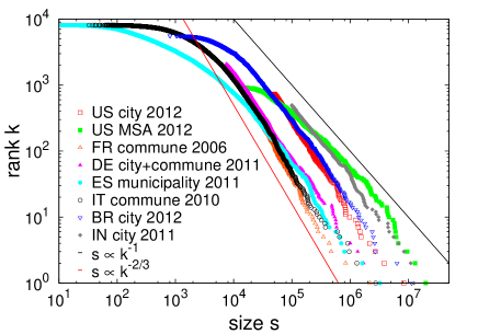
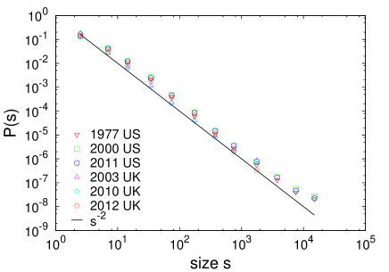
Figure 2: Left panel: Plot of size s with rank k of a city for different countries. The two straight lines are respectively $s\propto k^{-1}$ and $s\propto k^{-2/3}$, guides to the approximate extremes of the power law behavior of the data sets. Figure adapted from Ref. ghosh2014city . Right panel: Firm size distribution for USA US_firm_data and UK UK_firm_data .

VI.2 Scaling of urban measures

Analysis of available large urban data sets across decades for U.S.A. have concluded that (i) size is the major determinant, (ii) the space required per capita shrinks – the denser the settlement, the more intense is the use of infrastructure, (iii) all socio-economic activities accelerate, indicating higher productivity, and (iv) socio-economic activities diversify and become more interdependent. What comes as a surprise is that as city size increases, several quantities increase by small factor more than linear (superlinear scaling) bettencourt2007growth ; bettencourt2010unified . These relations were tested to be robust across a variety of urban measures, e.g., crime alves2013distance . A theoretical framework was developed bettencourt2013origins that derived the general properties of cities through the optimization of a set of local conditions, and was used to predict the average social, spatial and infrastructural properties of cities in a unified and quantitative way. A set of scaling relations were found that apply to all urban systems, supported by empirical data.

VI.3 Firms

Sizes of employment firms in terms of employees are known to follow the Zipf law axtell2001zipf , in a rather robust fashion compared to city sizes. Fig. 2 (right panel) shows the typical size distribution features in case of firms in USA and UK.

However, recent studies find that while the Zipf law holds good for the intermediate range, if one considers the firm assets, the power law which is usually attributed to a mechanism of proportional random growth, based on a regime of constant returns to scale. However the power law breaks down for the largest firms, which are mostly financial firms fiaschi2014interrupted . This deviation from the expected size, à la Zipf law, has been attributed to the shadow banking system, which can broadly be described as credit intermediation involving entities and activities outside the regular banking system. The identification of the correlation of the size of the shadow banking system with the performance of the financial markets through crashes and booms sheds some light on the reason for the financial crises that have struck the world in the recent times.

VII Consensus

Consensus is what many people say in chorus but do not believe as individuals.

– Abba Eban, Israeli politician (1915-2002)

Consensus in social systems is a very interesting subject in terms of it dynamics, as well as concerning conditions under which it can happen. Consensus is one of the most important aspects of social dynamics. Life presents many situations where it requires to assess shared decisions. Agreement leads to stronger position, giving it a chance to have an impact on society. The dynamics of agreement and disagreement among a collection of social being is complex. Statistical physicists working on opinion dynamics tend to define the opinion states of a population and the dynamics that determine the transitions between such states. In a typical scenario, one has several opinions (discrete or continuous) and one studies how global consensus (i.e., agreement of opinions) emerges out of individual opinions liggett1999stochastic ; deffuant2000mixing ; hegselmann2002opinion . Apart from the dynamics, the interest lies in the distinct steady state properties: a phase characterized by individuals widely varying in opinions and another phase where the majority of individuals have similar opinions.

VII.1 Voting

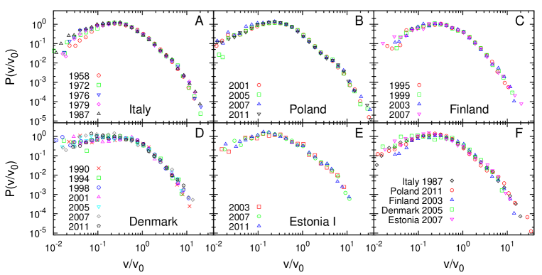
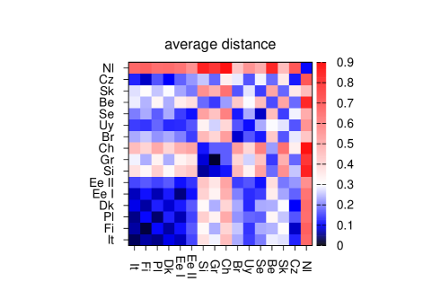
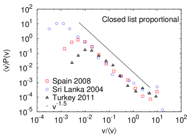
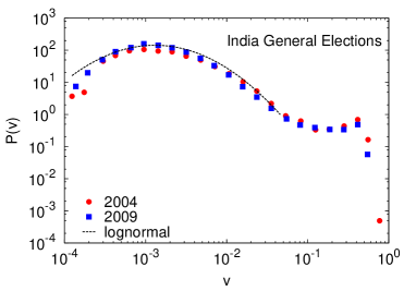
Figure 3: Top: Distribution of electoral performance of candidates in proportional elections with open lists. Middle: Quantitative assessment of the similarity between distributions between countries – The average K-S distance between distributions of electoral performance of candidates. Figures are adapted from Ref. chatterjee2013universality . Bottom Left: Probability distribution $P(v)$ of fraction of votes $v$ won by lists, rescaled by the average $\langle v\rangle$ for Closed List Proportional voting systems. The solid line indicates a power law decay of $v^{-1.5}$. Bottom Right: Probability distribution $P(v)$ of fraction of votes $v$ won by candidates in parliamentary elections of India, which follow majority rule voting.

The most common example of consensus formation in societies are in the process of voting. Elections are among the largest social phenomena, and has been well studied over years. There are many studies concerning turnout rates, detection of election anomalies, polarization and tactical voting, relation between party size and temporal correlations, relation between number of candidates and number of voters, emergence of third parties in bipartisan systems etc. Since the electoral system varies from country to country, there exists debates on the issue of which of the systems are more effective in capturing the view of the society. One of the many interesting questions one can ask is whether the distribution of votes is universal in a particular type of voting system. Recently it was shown that for open list proportional elections, the probability distribution of a performance of a candidate with respect to its own party list follows an universal lognormal distribution fortunato2007scaling , later confirmed by an extensive analysis of 53 data sets across 15 countries chatterjee2013universality . While the countries using open list proportional system do show universality, the rest follow different distributions showing little commonality within their patterns. In Fig. 3 (top panel) we show the data for countries which follow the lognormal pattern. The easiest way to see if distributions are similar, is to perform the Kolmogorov-Smirnov (K-S) test, where one can compute a distance measure to express how dissimilar a pair of probability distributions are. Fig. 3 (bottom panel) shows these distances. The countries at the left bottom corner, i.e., Italy, Finland, Poland, Denmark, Estonia I (elections held after 2002) are similar and their performance distributions known to be lognormal. Data from other countries are less similar to this set, and hence the computed K-S distances are much larger.

In closed list proportional system, votes are given to lists rather than candidates. Usually, the voting mechanism is complicated, with specific rules adopted by specific countries. What one can measure here is the fraction of votes $v$ given to a list. In Fig. 3 (Bottom Left), we show the rescaled (with average votes $\langle v\rangle$) plots for one election each of Spain, Sri Lanka and Turkey. What is interesting to observe is that the basic nature of the curves are similar, the range of the abscissa being dependent on the size of the constituencies. For a considerable range, the curves seem to follow a power law, approximately $v^{-1.5}$.

The majority rule or the first-past-the-post (FPTP) is a simple plurality voting system where the candidate with the maximum votes is declared the winner, and hence referred to as the winner takes all system. Usually, several political parties compete in a constituency, each nominating one candidate for the election. Hence, in practice, the list of candidates in a constituency consist of one each from all political parties contesting against one another. A voter casts a single vote in favor of the candidate of his/her choice. Under the FPTP system, the candidate with the maximum vote wins and is elected to the parliament. Fig. 3 (Bottom right) shows the distribution $P(v)$ of the fraction of votes $v$ received by a candidate in its constituency FPTPpaper . The curves are similar, with a log-normal peak in the bulk, indicative of an effective random multiplicative/branching process, and a second ‘leader-board’ peak around $v^{*}\approx 1/2$, indicative of the effective competition in a FPTP system. The gross feature of FPTP elections are similar except that the size and position of the leader-board peak indicated the effective competition in the political scenario.

Mathematical modeling would gain immensely from the information obtained from the empirical results. Having established the regularities for different election scenarios, one of the future challenges will be to develop statistical methodologies which can detect/indicate malpractices or even frauds in elections.

VII.2 Religion

A very debatable question is whether religion can be treated as a process of consensus formation? Viewing religious ideologies as opinion states, one can easily visualize the dynamics of religion – as in conversion, growth and decay in population due to change in the level of popularity, paradigm shift in beliefs, etc. Fig. 4 shows the rank plot of major religious affiliations. There has already been studies ausloos2007statistical relates to the size distribution of religious groups. The issue of inequality rises from the fact that religious representations are very much inhomogeneous across countries, the usual trend being the prevalence of one dominating religion or religious ideology. The cultural aspects, which are highly correlated with religious ideology shapes the social conditions and level of integration between various groups.

Figure 4: The rank plot of the number of religious adherents – numbers of different sub groups. Data taken from Ref. rel1 .

VII.3 Modeling opinion and its dynamics

Statistical physics has been used extensively in modeling opinion and its dynamics holyst2002social ; san7binary ; stauffer2009opinion ; sobkowicz2009modelling ; weisbuch2006 ; Castellano:2009 . The crucial step in modeling opinion is to assign the opinion ‘states’. In situations of binary choice, the Ising model paradigm seems to work, while situations with multiple choices can be modeled in various ways, e.g. Potts spin model for discrete case, or a continuous variable defined within a certain range of real numbers.

VII.3.1 Discrete opinion models

Among the earliest models proposed to describe opinion formation in a society is the voter model clifford1973model ; liggett1985interacting , where opinions can assume two values, $0$ and $1$ or $-1$ and $+1$. At each step of dynamics a randomly chosen individual is assigned the opinion of one of its randomly chosen nearest neighbors, independent of the original opinion state. The model represents a society where agents only imitate others. This model has similarities with the Ising model at zero temperature, where the states of the spins evolve depending to the states of the neighbors. But, since a random neighbor is chosen, the probability that any particular opinion is chosen is proportional to the number of neighbors having that opinion state, which is different from the Ising model, in which the probabilities depend exponentially on that number. For dimension $d>2$, no consensus can be reached for infinite systems, while in finite lattices consensus is asymptotically reached. However, for $d\leq 2$, it is possible to reach a consensus.

The Sznajd model sznajd2000opinion was motivated by the phenomenon of social validation, i.e., agents are influenced by groups rather than individuals. In a one-dimensional lattice, a pair of neighboring spins influence the opinion of their other neighbors in a particular way. In its original version, the rules of dynamic evolution were defined as:

• if $s_{i}s_{i+1}=1$, then $s_{i-1},s_{i+2}$ assumes the opinion of $s_{i}$

• if $s_{i}s_{i+1}=-1$, then $s_{i-1}$ assumes the opinion of $s_{i+1}$, $s_{i+2}$ the opinion of $s_{i}$.

In the majority-rule model galam2002minority a group of size $R$ is randomly chosen and the opinion state which is the majority in that group is assigned to all these $R$ individuals, $R$ being a random variable. One of the ‘favored’ opinions is adopted when there is a tie. Depending on the initial configuration, the final state is $+1$ or $-1$ for all opinions. Let the favored opinion be $+1$. It was shown that if one starts initially with $p$ fraction of opinions equal to $+1$, then a phase transition occurs at $p_{c}$ – for $p>p_{c}$, the final state is all $+1$. $p_{c}$ is dependent on the maximum size of a group. It was shown that $p_{c}$ could be less than $1/2$, which means that an initial minority can win in the end. The bias is possibly the reason for this, and was termed ‘minority spreading’. However, if only odd-sized groups are allowed, $p_{c}=1/2$. This model framework has been used with minor modifications to explain hierarchical voting, multi-species competition, etc. (see Ref. galam2008sociophysics for details). The problem with constant (odd) $R$ was solved in the mean-field limit krapivsky2003dynamics , where the group can be formed with randomly selected agents. The consensus time was found to be exactly $\ln N$ for $N$ agents. In $d=1$, where the opinions are not conserved, it was reported that the density of domains decay according to $t^{-1/2}$ so that the time to consensus is $\mathcal{O}(N^{2})$. In $d>1$ there is a broad distribution of the consensus times in higher dimensions and the most probable time to reach consensus shows a power-law dependence on $N$ with an exponent which depends on $d$. The upper critical dimension is claimed to be greater than $4$ and in dimensions greater than one there are always two characteristic timescales present in the system.

VII.3.2 Continuous opinion models

One of the important models using opinion as a continuous variable is the Deffuant model, uses the idea of ‘bounded-confidence’ deffuant2000mixing . In a model where a pair of individuals simultaneously change their opinions, it was assumed that two agents interact only if their opinions are close enough, as in people sharing closer points of view would interact more. Let $o_{i}(t)$ be the opinion of the individual $i$ at time $t$. An interaction of the agents $i$ and $j$ agents, who are selected randomly, would make the opinions update according to

$$o_{i}(t+1) = o_{i}(t)+\mu[o_{j}(t)-o_{i}(t)],$$ (25)

$$o_{j}(t+1) = o_{j}(t)+\mu[o_{i}(t)-o_{j}(t)],$$

where $\mu$ is a constant ($0\leq\mu\leq 0.5$), known as the ‘convergence parameter’. The total opinion remains constant and bounded, i.e., $o_{i}$ lies in the interval $[0,1]$. There is no randomness in the original model except the random choice of the agents who interact. Obviously, if $o_{j}>o_{i}$, $o_{i}$ becomes closer to $o_{j}$. If $\delta$ is the ‘confidence level’ (agents interact when their opinions differ by a quantity not more than $\delta$), the final distribution of opinions is dependent on on the values of $\delta$ and $\mu$. The possibilities are: (i) all agents may attain a unique opinion value, which is a case of consensus. It has been reported that the threshold value of $\delta$ above which all agents have the same opinion in the end is $1/2$, and is independent of the underlying topology fortunato2004universality . (ii) Convergence is reached with only two opinions surviving, a case of ‘polarization’. (iii) It can happen that the final state has several possible opinions: a state of ‘fragmentation’.

Hegselmann and Krause hegselmann2002opinion generalized the Deffuant model, where an agent simultaneously interacts with all other agents who have opinions within a prescribed bound. Instead of the convergence parameter, the simple average of the opinions of the appropriate neighbors is adopted. As a result, consensus is enhanced by making the bound larger. In case of a graph, the value of the consensus threshold is seen to depend on the average degree. In these models, starting from continuous values, the final opinions are discretized.

Another class of models employ a kinetic exchange like framework toscani2006kinetic . Including a diffusion term that takes care of the fact that agents can be randomly affected by external factors and subsequently change their opinion. The opinions $o_{i}$ and $o_{j}$ evolve following

$$o_{i}(t+1) = o_{i}(t)+\gamma\mathcal{P}(|o_{i}|)[(o_{j}(t)-o_{i}(t))+\eta_{i}\mathcal{D}(|o_{i}|)],$$ (26)

$$o_{j}(t+1) = o_{j}(t)+\gamma\mathcal{P}(|o_{j}|)[(o_{j}(t)-o_{i}(t))+\eta_{j}\mathcal{D}(|o_{j}|)],$$

where $\gamma\in[0,1/2]$ represents compromise propensity and $\eta$ is drawn from a random distribution with zero mean. As in the bounded-confidence models, the opinion of an agent will tend to decrease or increase so as to be closer to the opinion of the other. it is important to note that even if the diffusion term is absent, the total opinion is not conserved unless $P(o)$ is a constant. The functions $\mathcal{P}(.)$ and $\mathcal{D}(.)$ take care of the local relevance of the compromise and diffusion terms respectively. The choice of the functional forms of $\mathcal{P}$ and $\mathcal{D}$ decides the final state.

Another simpler model lallouache2010opinion considers binary interactions, where the opinions evolve as:

$$o_{i}(t+1)=\lambda[o_{i}(t)+\epsilon o_{j}(t)],$$ (27)

$$o_{j}(t+1)=\lambda[o_{j}(t)+\epsilon^{\prime}o_{i}(t)],$$

where $\epsilon,\epsilon^{\prime}$ are drawn randomly from uniform distributions in $[0,1]$. $o_{i}(t)$ is the opinion of individual $i$ at time $t$, and $o_{i}\in[-1,+1]$, and are also bounded, i.e.,. if $o_{i}$ exceeds $1$ or becomes less than $-1$, it is set to $1$ and $-1$, respectively. The parameter $\lambda$ is interpreted as ‘conviction’, and this models a society in where everyone has the same value of conviction. The model lacks conservation laws. The order parameter is defined as $O=|\sum_{i}o_{i}|/N$, the magnitude of the average opinion in a system with N agents. One also measures the fraction of the agents having $o_{i}=\pm 1$, called the condensation fraction $p$ Numerical simulations indicate that the system goes into either of the two possible phases: for any $\lambda\leq\lambda_{c}$, $o_{i}=0$ $\forall i$, while for $\lambda>\lambda_{c}$, $O>0$ and $O\to 1$ as $\lambda\to 1$ with $\lambda_{c}\simeq 2/3$, $\lambda_{c}$ is the ‘critical point’ of this phase transition. The critical point is easily confirmed by mean field calculation biswas2011phase . Using a fixed point equation $o^{*}[1-\lambda(1+\langle\epsilon\rangle)]=0$, the fixed point turns out to be $\lambda_{c}=1/(1+\langle\epsilon\rangle)$. For a random uniform distributed $\epsilon$ with $\langle\epsilon\rangle=1/2$, one can easily see, $\lambda_{c}=2/3$.

Several variants including the discrete version biswas2011mean , and the generalized version with a second parameter ‘influence’ sen2011phase gave further insights to the class of models. In another model biswas2012disorder , where negative influence was also considered, one could consider both discrete and continuous versions, which gave interesting insight into competing views and phase transitions.

All of the above models, which show a phase transition, can be viewed to correspond to broad distributions of opinions/consensus variables near their critical point. It is much easier to visualize a percolation stauffer1991introduction picture, where the sizes of percolation clusters have a power-law distribution close to the percolation phase transition. The alternative picture is that of self-organized criticality bak1997nature , where the activity size is also power law distributed.

VIII Bibliometrics

Academic publications (papers, books etc.) form an unique social system consisting of individual publications as entities, containing bibliographic reference to other older publications, and this is commonly termed as citation. The number of citations is a measure of the importance of a publication, and serve as a proxy for the popularity and quality of a publication. There has already been a plethora of empirical studies on citation data Sen:2013 , specifically on citation distributions Shockley:1957 ; Laherrere:1998 ; Redner:1998 ; Radicchi:2008 of articles, time evolution of probability distribution of citation Rousseau:1994 ; Egghe:2000 ; Burrell:2002 , citations for individuals Petersen:2011 and even their dynamics Eom:2011 , and the modeling efforts on the growth and structure of citation networks have produced a huge body literature in network science concerning scale-free networks Price:1965 ; barabasi1999emergence ; caldarelli2007scale .

The bibliometric tool of citation analysis is becoming increasingly popular for evaluating the performance of individuals, research groups, institutions as well as countries, the outcomes of which are becoming important in case of offering grants and awards, academic promotions and ranking, as well as jobs in academia, industry and otherwise. Since citations serve as a crucial measure for the importance and impact of a research publication, its precise analysis is extremely important. It is quite usual to find that some publications do better than others due to the inherent heterogeneity in the quality of their content, the gross attention on the field of research, the relevance to future work and so on. Thus different publications gather citations in time at different rates and result in a broad distribution of citations. For individual publications, the present consensus is that while most part of the distribution fit to a lognormal Shockley:1957 ; Redner:2005 , the extreme tail fits to a power law close to $3$ Redner:1998 ; peterson2010nonuniversal . This inequality in citations and other associated bibliometric indicators has been a field of interest to scientists in the last few decades.

There has also been studies that address the most popular papers, most cited scientists, and even Nobel prizes, which are awarded for groundbreaking discoveries, which change the face of science for ever. The laureates belong to the elite, and the papers which are identified to be the ones declaring the ‘discovery’ are timeless classics by their own right. Speaking in terms of inequality, these discoveries are indeed rare, and belong to the extreme end of the spectrum of all the associated work done in a field, some leading to the discoveries themselves, others complementing them, naturally true for the Nobel prize winning papers. However, there are limitations to the prize itself, defined by the number of discoveries that can be recognized and number of recipients in a single year in a given discipline. It has been observed that the delay between the discovery and the recognition as a Nobel prize is growing exponentially fortunato2014growing ; becattini2014nobel , the most rapidly in Physics, followed by Chemistry and Physiology or Medicine. As a result the age of a laureate at the time of the award is also increasing, seen to be exponential. Comparison with the average life expectancy of individuals concluded that by the end of this century, potential Nobel laureates in physics and chemistry are most likely to expire before being awarded and recognized.

In recent times, big team projects have dominated some of the frontline areas of science, in astrophysics, biology, genetics, quantum information etc. One can easily see that there has been a gorss inequality in the number of researchers who coauthor a paper milojevic2014principles .

In what follows, we will limit our discussion to some interesting aspects related to analysis of citations.

VIII.1 Annual citation indices

One of the quantities of major interest is the nature of the tail of the distribution of annual citations (AC) and impact factor (IF). IF are calculated annually for journals which are indexed in the Journal Citation Reports JCR . The precise definition is the following: if papers published in a journal in years $T-2$ and $T-1$ are cited ${\mathcal{N}}(T-2)+{\mathcal{N}}(T-1)$ times by the indexed journals in the year $T$, and $N(T-2)+N(T-1)$ are the number of ‘citable’ articles published in these years, the impact factor in year $T$ is defined as

$$I(T)=\frac{{\mathcal{N}}(T-2)+{\mathcal{N}}(T-1)}{N(T-2)+N(T-1)}.$$ (28)

The number of annual citations (AC) $n(T)$ to a journal in a given year is

$$n(T)=\sum_{t\leq T}{\sum_{i}{\mathcal{A}}_{i}(t,T)},$$ (29)

where ${\mathcal{A}}_{i}(t,T)$ is the number of citations received in the year $T$ by the $i$th paper published in the year $t\leq T$.

Another measure, $r(T)$, the annual citation rate (CR) at a particular year $T$ that is defined khaleque2014evolution as annual citations divided by the number of articles published in the same year, i.e.,

$$r(T)=n(T)/N(T).$$ (30)

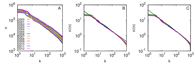
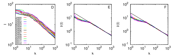
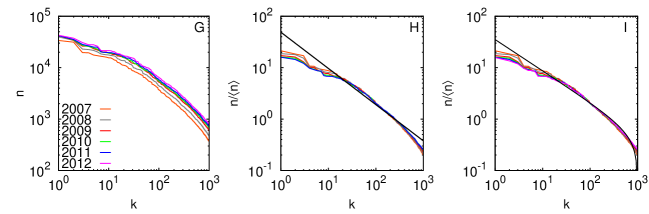
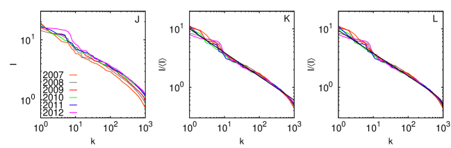
Figure 5: Plots of annual citation $n$ and impact factor $I$ with rank $k$: (A) Rank plot of the top $1000$ journals, ranked according to citations, scaling collapse of the same (B) showing a Zipf law fit: $f(x)=Ax^{-b_{n}}$, with $b_{n}=0.70(2)$ and (C) showing a two-exponent Zipf law fit: $f(x)=k(N+1-x)^{a_{n}}/x^{b_{n}}$, with $a_{n}=0.27(2)$ and $b_{n}=0.69(2)$. (D) rank plot of the top $1000$ journals, ranked according to impact factors, and scaling collapse of the same (E) showing a Zipf law fit: $g(x)=Ax^{-b_{I}}$, with $b_{I}=0.54(1)$ and (F) showing a two-exponent Zipf law fit: $f(x)=k(N+1-x)^{a_{I}}/x^{b_{I}}$, with $a_{I}=0.03(2)$ and $b_{I}=0.56(2)$. The data is from SCI sets. SOCSCI data: (G) Rank plot of the top $1000$ journals, ranked according to citations, scaling collapse of the same (H) showing a Zipf law fit: $f(x)=Ax^{-b_{n}}$, with $b_{n}=0.7043\pm 0.001$ and (I) showing a two-exponent Zipf law fit: $f(x)=k(N+1-x)^{a_{n}}/x^{b_{n}}$, with $a_{n}=0.47(2)$ and $b_{n}=0.61(2)$. (J) rank plot of the top $1000$ journals, ranked according to their impact factors, scaling collapse of the same (K) showing a Zipf law fit: $f(x)=Ax^{-b_{I}}$, with $b_{I}=0.40(1)$ and (L) showing a two-exponent Zipf law fit: $f(x)=k(N+1-x)^{a_{I}}/x^{b_{I}}$, with $a_{I}=0.06(2)$ and $b_{I}=0.39(2)$. The figure is adapted from Ref. khaleque2014evolution .

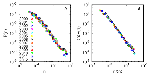
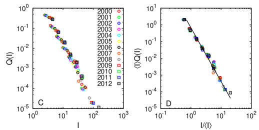
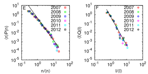
Figure 6: (A) Probability distribution of annual citations $P(n)$ (B) its scaling collapse, for the top $1000$ journals ranked according to citations. It fits fairly well to a power law $Bx^{-\gamma_{n}}$; the straight line corresponds to $\gamma_{n}=2.52$ in the log-log plot; (C) probability distribution of impact factor $Q(I)$ (D) its scaling collapse, for the top $1000$ journals ranked according to impact factor. The straight line corresponds to $\gamma_{I}=3.16$. The data are for SCI sets. (E) Scaling collapse of probability distribution of annual citations $P(n)$ for the top $1000$ journals ranked according to citations; power law fit with $\gamma_{n}=2.42$; (F) Scaling collapse of probability distribution of annual citations $P(n)$ for the top $1000$ journals ranked according to impact factor; power law fit with $\gamma_{I}=3.50$. The data are from SOCSCI sets. The figure is adapted from Ref. khaleque2014evolution .

Extensive studies on the historical behavior of the IF ranked distribution Popescu:2003 ; Mansilla:2007 have established the behavior of the low ranked (large $k$) journals and the precise nature of the distribution function. Study of a limited sample of the top $1000$ ranked ($k\leq 1000$) Science journals (SCI) reveal that the distributions remain invariant with time, seen by rescaling the plots by their averages. For small ranks, the citations are almost independent of the ranks implying a cluster of journals with comparable citations that occupy the top positions (Fig. 5A, B). Fitting the curves for $k>10$ by $f(x)\sim x^{-b_{n}}$ it was found that $b_{n}=0.70(2)$. Similarly, for the IF, the scaled data seemed to fit to the same form with an exponent $b_{I}=0.54(1)$ (Fig. 5D, E). These Zipf exponents as they are obtained from the rank plots. For Social Science (SOCSCI), approximate power law fits are possible for the rank plots with Zipf exponents $b_{n}=0.70(2)$ and $b_{I}=0.40(1)$ respectively (Fig. 5F, H).

The single exponent fitting on the tail does not justify the observed bending of the real data (Fig. 5B, E, H, K), but the curves can be as well be fitted nicely to a function with two exponents $f(x)=k(N+1-x)^{a}/x^{b}$, where $N$ represents the rank-order data; $a$ and $b$ are two exponents to fit Mansilla:2007 . For the citation data, $b_{n}=0.69(2)$ and $a_{n}=0.27(2)$ (Fig. 5C). Similarly, for IF data the exponents are $b_{I}=0.56(2)$ and $a_{I}=0.03(2)$ (Fig. 5F). For SOCSCI data the exponents are $b_{n}=0.61(2)$, $a_{n}=0.47(1)$, $b_{I}=0.39(2)$, and $a_{I}=0.06(1)$ (Fig. 5I, L). $a_{I}$ is close to zero for (Fig. 5F, L) implying that the power law fit is rather accurate, while for (Fig. 5C, I), the two exponents fit appears to be more appropriate.

The probability distribution of both annual citations and impact factors showed monotonic decays and their tails can be fitted to power law forms. The plots showed excellent scaling collapse for different years when the probability distributions are rescaled by their averages. For annual citations, the lower values hint towards a lognormal but the ‘tail’ of the distribution seems to fit to a power law Golosovsky:2012 . The power law exponents are $\gamma_{n}$ and $\gamma_{I}$ are $2.52(1)$ and $3.16(1)$ respectively. The Zipf exponent $b$ as obtained from a rank plot relates to the exponent of the probability distribution $\gamma$ as $\gamma=1+1/b$ Clauset:2009 . Using the values of $b$ obtained, the values of $\gamma$ are found to be $2.42$ and $2.85$ respectively for AC and IF, quite consistent with the values obtained directly from the distributions (Fig. 6). The same holds true for the SOCSCI data (expected Pareto exponents are $2.42$ and $3.50$ from the rank plots compared to the best fit values $2.32(2)$ and $3.13(2)$). However, it is apparent that there could be some corrections to the power law scaling. The distribution of the annual citation rate (CR) $r$ is also broad, but non-monotonic, with a peak around half the average value. The distributions fit well to log-Gumbel distributions khaleque2014evolution .

VIII.2 Universality in citation distributions

Back in 1957, Shockley Shockley:1957 first claimed that the scientific publication rate is dictated by lognormal distribution. Later evidences based on analysis of records for highly cited scientists indicate that the citation distribution of individual authors follow a stretched exponential Laherrere:1998 . Another analysis of the data from ISI claims that the tail of the citation distribution has a power law decay with an exponent close to $3$ Redner:1998 , What followed was a meticulous analysis of 110 years of data from Physical Review, concluding that most of the citation distribution fits remarkably well to a lognormal Redner:2005 . However, it is now well agreed that most of the distribution fits to a lognormal but the tail fits to a power law peterson2010nonuniversal .

The distribution of citations of individual publications within a single discipline is seen to be quite broad – some papers get very little citations, a few collect huge citations, but there are many who collect an average number of citations. The average number of citations gathered in a discipline is strongly dependent on the discipline itself. It has been observed Radicchi:2008 that if one can rescale the absolute number of citations $c$ by the average in that discipline $\langle c\rangle$, the relative indicator $c_{f}=c/\langle c\rangle$ has a functional form independent of the discipline. The rescaled probability distribution fits well to a lognormal for most of its range.

One can also ask the question that what happens for academic institutions, where the quality of scientific output measured in terms of the total number of publications, total citations etc. can vary widely across the world. In the popular notion, there are institutions which are known to ‘better’ than others, and in fact, rankings go exist among them. One can ask if the nature of the world’s best institutions’ output is different from the more average ones. It is found that all institutions have a wide distribution of citations to their publications, with a functional form that is independent of their rankings chatterjee2014universality . To see this, one has to use a relative indicator $c_{f}=c/\langle c\rangle$ again. The scaling function fits to a lognormal for most of its range, while the highest cited papers deviate to fit to a power law tail.

Now, how does the same look at the level of journals? It is quite well known in popular perception that journals present a wide variety in terms of impact factor and annual citations, as also reported in critical studies khaleque2014evolution ; Popescu:2003 ; Mansilla:2007 . The natural question to ask is whether the universality that exists across disciplines or academic institutions prevail also for journals. It seems that this is not the case in reality. In fact, it is seen that there are at least two classes of journals, a General class, which comprises the most popular standard journals, and an Elite class consisting a very small group of highly reputed journals characterized by high impact factor and average citations chatterjee2014universality . The former class is characterized by a lognormal distribution in the bulk, which the latter is characterized by a strong tendency of divergence as $1/c$ at small values of citations, with no clear indication of lognormal bulk. However, for both these classes, the distribution of the highest cited papers decay a power law tail with an exponent close to $3$.

IX Networks

Networks have been a subject of intense study in the last 2 decades, and drawn researchers from a variety of disciplines to study the structural, functional, dynamical and various aspects of them, uncovering new patterns and understanding interesting phenomena from physics, biology, computer science and social sciences newman2006structure . The studies of the internet and the web has led to engineering faster routing strategies and developing efficient search engines, biological networks have given insight into the functional elements in bio-chemical processes inside organisms, provided tools for complex experiments, that in social networks has bettered our understanding about spreading of innovations, rumors and even epidemics, leading to devising strategies to make them either more efficient or less efficient according to the case it may be.

Studies of the World Wide Web albert1999internet ; broder2000graph , the internet faloutsos1999power , citation networks Price:1965 ; Redner:1998 , email network ebel2002scale , network of human sexual contacts liljeros2001web all show power law tail in the degree distributions for a large range of values, similar to metabolic networks jeong2000large and protein-protein interaction network uetz2000comprehensive .

Studies on massive and popular social networks like Facebook ugander2011anatomy has shown broad distributions with tails resembling power laws. Experiments done by setting up social networks of communication have shown that the network slowly evolves and the shape of the degree distribution stabilizes with time kossinets2006empirical , with characteristics similar to other massive networks, such as clustering and broad degree distribution with power law tail. Since then, almost all possible online social networks have been analyzed, and most of them have been found to have a power law degree distribution (see e.g., Ref. li2014sparse ).

X Measuring inequality

Socio-economic inequalities can be quantified in several ways. The most common measures are absolute, in terms of indices, e.g., Gini gini1921measurement , Theil theil1967economics indices. Alternatively one can use a relative measure, by considering the probability distributions of various quantities, whereas the indices can be computed easily from the distributions themselves. The quantity in question in the socio-economic context usually displays a broad distribution, like lognormals, power-laws or their combinations. For instance, the distribution of income is usually an exponential followed by a power law druagulescu2001exponential (see Ref.chakrabarti2013econophysics for other examples).

The Lorenz curve Lorenz is a function representing the cumulative proportion $X$ of (ordered from lowest to highest) individuals in terms of the cumulative proportion of their sizes $Y$. $X$ can be anything like income or wealth, citation, votes, city population etc. The Gini index ($g$) is commonly defined as the ratio of (i) the area enclosed between the equality line and the Lorenz curve, and (ii) the area below the equality line. If the area between (i) the Lorenz curve and the equality line is given by $A$, and that (ii) under the Lorenz curve is given by $B$ (See Fig. 7), the Gini index is simply defined as $g=A/(A+B)$. It is a very common measure to quantify socio-economic inequalities. Ghosh et al. ghosh2014inequality recently introduced a new measure, called ‘$k$ index’ (where ‘$k$’ stands for the extreme socio-economic inequalities in Kolkata), defined as the fraction $k$ such that $(1-k)$ fraction of people or papers possess $k$ fraction of income/wealth or citations respectively.

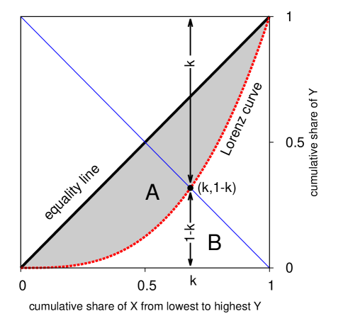
Figure 7: Schematic representation of Lorenz curve, Gini index $g$ and $k$ index. The dashed red line stands for the Lorenz curve and the black solid line represents perfect equality. The area enclosed by the equality line and the Lorenz curve is $A$ and that below the Lorenz curve is $B$. The Gini index is given by $g=A/(A+B)$. The $k$ index is given by the abscissa of the intersection point of the Lorenz curve and $Y=1-X$.

When the probability distribution is described by an appropriate parametric function, one can derive, using mathematical techniques, these inequality measures as a function of those parameters analytically. Several empirical evidence show that the distributions can be put into a few types, most of which turn out to be a mixture of two distinct parametric functions with a single crossover point inoue2014measuring

$$P(m)=F_{1}(m)\theta(m,m_{\times})+F_{2}(m)\Theta(m-m_{\times}),$$ (31)

where $\theta(m,m_{\times})\equiv\Theta(m)-\Theta(m-m_{\times})$, $m_{\times}$ is the crossover point and $F_{1}$, $F_{2}$ being the two functions. For these, it is possible to compute the general form of the Lorenz curve, Gini index $g$ and $k$ index. It is also easy to check the values obtained from empirical calculations with those from analytical expressions for consistency. By minimizing the gap between the empirical and analytical values of the inequality measures, one can numerically enumerate of the crossover point which is usually determined by eye estimates.

XI How to deal with inequality?

So distribution should undo excess, and each man have enough.

[King Lear, Act 4, Scene 1] – William Shakespeare, English playright and writer (1564-1616)

In this section, we will not discuss socio-political theories such as socialism in it different forms, and rather give an objective view of generalized processes that can be adopted to decrease inequalities.

One of the long studied problems that deals with the issue of socio-economic inequality is that of efficient allocation of resources. An inefficient allocation process may lead to unequal distribution of resources which in course of time goes through a reshuffling and multiplicative process, and finally result in a very skew distribution. We will discuss in the following, how statistical physics can help in modeling processes that produce fairly equal distributions.

Most resources are limited in supply, and hence, efficiently allocating them is therefore of great practical importance in many fields. Resources may be either physical (oil, CPUs, chocolates) or immaterial (time, energy, bandwidth), and allocation may happen instantaneously or over a long period. Thus, there is no universal method that solves all allocation problems. In addition, the variety of situations that people or machines (generically called “agents”) face, require specific modeling in a first step. However, two features connect all these situations: when resources are scarce, the agents compete for them; when competing repeatedly, the agents learn and become adaptive. Competition in turn has two notable consequences. The agents have a strong incentive to think and act as differently as possible Arthur , that is, to become heterogeneous. Additionally, competition implies interaction, because the share of resources that an agent obtains depends on the actions of other agents.

While multi-agent modeling in the context of Game theory helps, even simpler modeling using the framework of statistical physics chakraborti2013statistical helps in a deeper understanding of the problem using a framework which is very different from those traditionally used by mainstream social scientists. While some models have already been proposed and efficiently utilized in certain fields, there is further need of developing novel and efficient models for a variety of problems.

The optimal allocation of resources is an issue of utmost concern in economic systems. Formalized as the simultaneous maximization of the utility of each member of the economy over the set of achievable allocations, the main issue is that individuals have typically conflicting goals, as the profit of one goes against that of the others. This makes the nature of the problem conceptually different from optimization problems where usually a single objective function has to be maximized. Markets, under some conditions, can solve this problem efficiently – prices adjust in a self-organized manner to reflect the true value of the good.

There have been recent attempts to model and describe resource allocation problems in a collection of individuals within a statistical mechanics approach. The focus is on competitive resource allocation models where the decision process is fully decentralized, that is, communication between the agents is not explicit. Interaction plays a crucial role and give rise to collective phenomena like broad distribution of fluctuations, long memory and even phase transitions. Additionally, the agents usually act very differently from one another, and sometimes have the ability to change actions according to the need their goals. This implies strong heterogeneity and non-equilibrium dynamics, ingredients which are extremely appealing to physicists, who possess the tools and concepts that are able to analyze and possibly solve the dynamics of such systems. The essential difference lies in the behavior of the constituent units, while particles, electrons cannot think and act, social units sometime do, which adds to the complexity.

Let us consider a population of $N$ agents and $R$ resources, which they try to exploit. Generically, $R$ denotes the number of possible choices of the agents, which naturally means $R\geq 2$. For the simplest case $R=2$, agents must choose which resource to exploit. The El Farol Bar Problem (EFBP) Arthur : $N$ customers compete for $L<N$ seats at the bar. At every time step, they must choose whether to go to the bar or to stay at home. The Minority Game (MG) CZ97 simplifies the EFBP in many respects by taking $L=N/2$. The Kolkata Paise Restaurant problem (KPR) assumes that the number of resources scales with $N$, in which $R$ restaurants have a capacity to serve only one customer each, so that the agents try to remain alone as often as possible Chakrabarti2009 .

The KPR Chakrabarti2009 ; Ghosh2010 problem is similar to various adaptive games (see Challet2004 ) but uses one of the simplest scenario to model resource utilization in a toy model paradigm. The simplest version has $N$ agents (customers) simultaneously choosing equal number $R$ ($=N$) of restaurants, each of which serve only one meal every evening, and hence, showing up in a place with more people gives less chance of getting food. Utilization is measured by the fraction of agents $f$ getting a meal or equivalently, by measuring the complimentary quantity: the fraction ($1-f$) of meals wasted, because some of the restaurants do not get any customer at all. An entirely random occupancy algorithm sets a benchmark of $f=1-1/e\approx 0.63$. However, a crowd-avoiding algorithm Ghosh2010 can improve the utilization to around $0.8$. If ones varies the ratio of agents to restaurants $(N/R)$ below unity, one can observe a phase transition – from an ‘active phase’ characterized by a finite fraction of restaurants $\rho_{a}$ with more than one agent, and an ‘absorbed phase’, where this quantity $\rho_{a}$ vanishes Ghosh2012 . Adapting the same crowd avoiding strategy in a version of the Minority Game where the extra information about the crowd was provided, one could convergence to the steady state achieve in a very small time, $O(\log\log N)$ Dhar2011 . In another modification to this problem Biswas2012 , one could observe a phase transition depending on the amount of information that is shared. The main idea for the above studies was to use iterative learning to find simple algorithms that could achieve a state of maximum utilization in a very small time scale. Although this review touches upon topics seemingly discrete from one another, some of the processes are interlinked, e.g., resource utilization can be seen as a key ingredient to city growth and the broad distribution of city sizes ghosh2014zipf .

XII Discussions

Socio-economic inequalities have been around, manifested in several forms, since history. With time, the nature and extent of these have changed, sometimes for good, but mostly for worse. This is traditionally a subject of study of social sciences, and scholars have been looking upon the causes and effects from a sociological perspective, and trying to understand the consequences on the economics. In reality this is not so simple, at times the latter is what is responsible for the effect on the former, making the cause-effect interpretation much more complex.

At the opposite end, had the world been very equal, it would have been difficult to compare the extremes, separate the good from the bad, hardly any leaders people would look up to, lack stable governments if there were almost equal number of political rivals, etc.

Recently, there has been a lot of concern about the increase of inequality in income and wealth, as seen from different measurements piketty2014capital , and has in such, renewed the interest on this subject among the leading social scientists across the globe. However, energy use has been observed to become much more equal with time lawrence2013global . In the economics front, how inequalities affect financial markets, firms and their dynamics, and vice versa is an important area to look into. Objects which are directly affected by economy, industrialization and rapidly growing technologies, in terms of social organization of individual entities, as in urban systems, are becoming important areas of study. In climbing up and down the social ladder mervis2014tracking ; bardoscia2013social is something difficult to track, until recent surveys which provide some insight into the dynamics. Many deeper and important issues in society neckerman2004social still needs attention in terms of inequality research, available data and its further analysis can bring out hidden patterns which may be used to encounter those situations. The main handicap is the lack of data of good quality, and the abstractness of the issues, which may not always be easily amenable to statistical modeling.

Physicists’ interests are mostly concentrated on subjects which are amenable to macroscopic or microscopic modeling, where tools of statistical physics prove useful in explaining the emergence of broad distributions. A huge body of literature has been already developed, containing serious attempts to understand socio-economic phenomena, branded under Econophysics and Sociophysics chakrabarti2007econophysics . The physics perspective brings new ideas and an alternative outlook to the traditional approach taken by social scientists, and is seen in the increasing collaborations across disciplines lazer09 .

- [1] D. Lazer, A. Pentland, L. Adamic, S. Aral, A.-L. Barabási, D. Brewer, N. Christakis, N. Contractor, J. Fowler, M. Gutmann, T. Jebara, G. King, M. Macy, D. Roy, and M. Van Alstyne. Computational social science. Science, 323(5915):721–723, 2009.
- [2] P. Ball. Critical mass. Farrar, Straus and Giroux, New York, USA, 2004.
- [3] L. Bachelier. Théorie de la spéculation. Gauthier-Villars, 1900.
- [4] E. Majorana. Il valore delle leggi statistiche nella fisica e nelle scienze sociali. Scientia, 36:58–66, 1942.
- [5] L. P. Kadanoff. From simulation model to public policy an examination of forrester’s urban dynamics. Simulation, 16(6):261–268, 1971.
- [6] E. W. Montroll and W. W. Badger. Introduction to quantitative aspects of social phenomena. Gordon & Breach, New York, 1974.
- [7] P. W. Anderson, K. Arrow, and D. Pines. The economy as an evolving complex system. Addison-Wesley, Redwood City, 1988.
- [8] M. Buchanan. To understand finance, embrace complexity. http://www.bloomberg.com/news/2013-03-10/to-understand-finance-embrace-complexity.html, March 11, 2013.
- [9] M. Buchanan. The social atom. Marshall Cavendish Business, London, UK, 2007.
- [10] Institute for New Economic Thinking. http://ineteconomics.org/.
- [11] K. Neckerman, editor. Social inequality. Russell Sage Foundation, 2004.
- [12] E. Pennisi. Our egalitarian eden. Science, 344(6186):824–825, 2014.
- [13] M. Buchanan. More equal than others. Nature Phys., 10(7):471–471, 2014.
- [14] A. Chatterjee and B. K. Chakrabarti. Kinetic exchange models for income and wealth distributions. Eur. Phys. J. B, 60:135–149, 2007.
- [15] H. Pringle. The ancient roots of the 1%. Science, 344(6186):822–825, 2014.
- [16] B. K. Chakrabarti, A. Chakraborti, S. R. Chakravarty, and A. Chatterjee. Econophysics of income and wealth distributions. Cambridge Univ. Press, Cambridge, 2013.
- [17] C. Castellano, S. Fortunato, and V. Loreto. Statistical physics of social dynamics. Rev. Mod. Phys., 81:591–646, 2009.
- [18] D. Stauffer, S. Moss De Oliveira, P. M. C. de Oliveira, and J. S. Sá Martins. Biology, sociology, geology by computational physicists. Elsevier, Amsterdam, 2006.
- [19] D. Stauffer. A biased review of sociophysics. J. Stat. Phys., 151(1-2):9–20, 2013.
- [20] S. Galam. Sociophysics: a physicist’s modeling of psycho-political phenomena. Springer, 2012.
- [21] P. Sen and B. K. Chakrabarti. Sociophysics: An Introduction. Oxford Univ. Press, Oxford, 2014.
- [22] S. Sinha, A. Chatterjee, A. Chakraborti, and B. K. Chakrabarti. Econophysics: An Introduction. Wiley-VCH, Weinhein, 2010.
- [23] H. E. Stanley. Introduction to Phase Transitions and Critical Phenomena. Oxford Univ. Press, Oxford and New York, 1971.
- [24] S. Fortunato and C. Castellano. Scaling and universality in proportional elections. Phys. Rev. Lett., 99(13):138701, 2007.
- [25] A. Chatterjee, M. Mitrović, and S. Fortunato. Universality in voting behavior: an empirical analysis. Sci. Rep., 3:1049, 2013.
- [26] M. C. Mantovani, H. V. Ribeiro, M. V. Moro, S. Picoli Jr, and R. S. Mendes. Scaling laws and universality in the choice of election candidates. Europhys. Lett., 96(4):48001, 2011.
- [27] H. D. Rozenfeld, D. Rybski, J. S. Andrade, M. Batty, H. E. Stanley, and H. A. Makse. Laws of population growth. Proc. Natl. Acad. Sci., 105(48):18702–18707, 2008.
- [28] M. H. R. Stanley, L. A. N. Amaral, S. V. Buldyrev, S. Havlin, H. Leschhorn, P. Maass, M. A. Salinger, and H. E. Stanley. Scaling behaviour in the growth of companies. Nature, 379(6568):804–806, 1996.
- [29] R. N. Mantegna and H. E. Stanley. Introduction to Econophysics: Correlations and Complexity in Finance. Cambridge Univ. Press, Cambridge, 2000.
- [30] A. M. Petersen, J. Tenenbaum, S. Havlin, and H. E. Stanley. Statistical laws governing fluctuations in word use from word birth to word death. Sci. Rep., 2:313, 2012.
- [31] P. Bak. How Nature Works. Oxford Univ. Press, Oxford, 1997.
- [32] D.G. Champernowne. A model of income distribution. Econ. J., 63:318–351, 1953.
- [33] M. Mitzenmacher. A brief history of generative models for power law and lognormal distributions. Internet Maths., 1(2):226–251, 2004.
- [34] H. A. Simon. On a class of skew distribution functions. Biometrika, pages 425–440, 1955.
- [35] R. K. Merton. The matthew effect in science. Science, 159(3810):56–63, 1968.
- [36] G. U. Yule. A mathematical theory of evolution, based on the conclusions of dr. jc willis, frs. Phil. Trans. Roy. Soc. London B, 213:21–87, 1925.
- [37] M. E. J. Newman. Power laws, pareto distributions and zipf’s law. Contemporary Phys., 46(5):323–351, 2005.
- [38] D. de Solla Price. A general theory of bibliometric and other cumulative advantage processes. J. Am. Soc. Information Sc., 27(5):292–306, 1976.
- [39] D. de Solla Price. Networks of scientific papers. Science, 149(3683):510–515, 1965.
- [40] A. L. Barabási and R. Albert. Emergence of scaling in random networks. Science, 286(5439):509–512, 1999.
- [41] R. Albert and A. L. Barabási. Statistical mechanics of complex networks. Rev. Mod. Phys., 74(1):47–97, 2002.
- [42] S. N. Dorogovtsev and J. F. F. Mendes. Evolution of networks. Adv. Phys., 51(4):1079–1187, 2002.
- [43] A. Sen. Poverty and famines. Oxford Univ. Press, New Delhi, 1999.
- [44] M. Foucault. Le Pouvoir psychiatrique:Cours au College de France 1973- 74. Gallimard, Paris, 2003.
- [45] R. Scruton. Thinkers of the new left. Longman, Sussex, 1985.
- [46] J. Rawls. A Theory of Justice. Harvard Univ. Press, Cambridge, 1971.
- [47] V. Pareto. Cours d’economie politique. Rouge, Lausanne, 1897.
- [48] R. Gibrat. Les inégalités économiques. Paris, Sirey, 1931.
- [49] D.G. Champernowne and F.A. Cowell. Economic Inequality and Income Distribution. Cambridge Univ. Press, Cambridge, 1998.
- [50] E. W. Montroll and M. F. Shlesinger. On 1/f noise and other distributions with long tails. Proc. Natl. Acad. Sci., 79:3380–3383, 1982.
- [51] C. Gini. Measurement of inequality of incomes. Econ. J., 31(121):124–126, 1921.
- [52] R.V. Hogg, J.W. Mckean, and A.T. Craig. Introduction to mathematical statistics. Pearson Education, Delhi, 2007.
- [53] A. Chatterjee, S. Yarlagadda, and B. K. Chakrabarti, editors. Econophysics of Wealth Distributions. New Economic Windows Series, Springer-Verlag, Milan, 2005.
- [54] V.M. Yakovenko and J. Barkley Rosser Jr. Colloquium: Statistical mechanics of money, wealth and income. Rev. Mod. Phys., 81:1703–1725, 2009.
- [55] Internal Revenue Service (IRS) – Individual Tax Tables, retreived June, 2014. http://www.irs.gov/uac/SOI-Tax-Stats—Individual-Statistical-Tables-by-Size-of-Adjusted-Gross-Income.
- [56] Forbes, World’s Billionaires list, retreived July, 2014. http://www.forbes.com/billionaires/list/.
- [57] BitcoinRichList, retreived March, 2014. http://bitcoinrichlist.com.
- [58] International Monetary Fund, retreived June, 2014. http://www.imf.org/.
- [59] P. Richmond, S. Hutzler, R. Coelho, and P. Repetowicz. A review of empirical studies and models of income distributions in society. In B. K. Chakrabarti, A. Chakraborti, and A. Chatterjee, editors, Econophysics and Sociophysics: Trends and Perspectives, pages 131–159. Wiley-VCH, Weinheim, 2007.
- [60] W. Souma. Physics of personal income. In H. Takayasu, editor, Empirical Science of Financial Fluctuations: the Advent of Econophysics, pages 343–352. Springer, Tokyo, 2002.
- [61] T. Mizuno, M. Toriyama, T. Terano, and M. Takayasu. Pareto law of the expenditure of a person in convenience stores. Physica A, 387(15):3931–3935, 2008.
- [62] A. Ghosh, K. Gangopadhyay, and B. Basu. Consumer expenditure distribution in india, 1983–2007: Evidence of a long pareto tail. Physica A, 390(1):83–97, 2011.
- [63] M. Levy and S. Solomon. New evidence for the power law distribution of wealth. Physica A, 242:90–94, 1997.
- [64] S. Solomon and P. Richmond. Stable power laws in variable economies; lotka-volterra implies pareto-zipf. Eur. Phys. J. B, 27:257–261, 2002.
- [65] P. Richmond and S. Solomon. Power laws are boltzmann laws in disguise. Int. J. Mod. Phys. C, 12:333–343, 2001.
- [66] J-P. Bouchaud and M. Mézard. Wealth condensation in a simple model of economy. Physica A, 282:536–545, 2000.
- [67] A.A. Drăgulescu and V.M. Yakovenko. Statistical mechanics of money. Eur. Phys. J. B, 17:723–729, 2000.
- [68] A. Chakraborti and B. K. Chakrabarti. Statistical mechanics of money: how saving propensity affects its distribution. Eur. Phys. J. B, 17:167–170, 2000.
- [69] A. Chatterjee, B. K. Chakrabarti, and S. S. Manna. Pareto law in a kinetic model of market with random saving propensity. Physica A, 335:155–163, 2004.
- [70] M. N. Saha and B. N. Srivastava. A treatise on heat. Indian Press, Allahabad, 1931.
- [71] J. Angle. The surplus theory of social stratification and the size distribution of personal wealth. Soc. Forces, 65(2):293–326, 1986.
- [72] J. Angle. The inequality process as a wealth maximizing process. Physica A, 367:388–414, 2006.
- [73] A. Chatterjee. Kinetic models for wealth exchange on directed networks. Eur. Phys. J. B, 67(4):593–598, 2009.
- [74] L. Pareschi and G. Toscani. Interacting Multiagent Systems: Kinetic Equations and Monte Carlo Methods. Oxford Univ. Press, Oxford, 2013.
- [75] A. Banerjee and V.M. Yakovenko. Universal patterns of inequality. New J. Phys., 12:075032, 2010.
- [76] S. Lawrence, Q. Liu, and V. M. Yakovenko. Global inequality in energy consumption from 1980 to 2010. Entropy, 15(12):5565–5579, 2013.
- [77] A. Chatterjee, S. Sinha, and B. K. Chakrabarti. Economic inequality: Is it natural? Current Science, 92(10):1383–1389, 2007.
- [78] T. Piketty. Capital in the Twenty-first Century. Harvard Univ. Press, 2014.
- [79] T. Piketty and E. Saez. Inequality in the long run. Science, 344(6186):838–843, 2014.
- [80] M. Batty. The size, scale, and shape of cities. Science, 319(5864):769–771, 2008.
- [81] F. Auerbach. Das gesetz der bevölkerungskonzentration. Petermanns Geographische Mitteilungen, 59:74–76, 2008.
- [82] A. J. Lotka. Elements of physical biology. Williams & Wilkins, Baltimore, 1925.
- [83] H. W. Singer. The “courbe des populations”. a parallel to pareto’s law. Econ. J., 46(182):254–263, 1936.
- [84] G. K. Zipf. Human Behaviour and the Principle of Least-Effort. Addison-Wesley, Cambridge, 1949.
- [85] K. T. Rosen and M. Resnick. The size distribution of cities: an examination of the pareto law and primacy. J. Urban Econ., 8(2):165–186, 1980.
- [86] K. Gangopadhyay and B. Basu. City size distributions for india and china. Physica A, 388(13):2682–2688, 2009.
- [87] L. Benguigui and E. Blumenfeld-Lieberthal. Beyond the power law–a new approach to analyze city size distributions. Computers Envir. Urb. Sys., 31(6):648–666, 2007.
- [88] X. Gabaix. Zipf’s law for cities: an explanation. Quart. J. Econ., 114:739–767, 1999.
- [89] D. H. Zanette and S. C. Manrubia. Role of intermittency in urban development: a model of large-scale city formation. Phys. Rev. Lett., 79(3):523, 1997.
- [90] M. Marsili and Y. C. Zhang. Interacting individuals leading to zipf’s law. Phys. Rev. Lett., 80(12):2741, 1998.
- [91] A. Blank and S. Solomon. Power laws in cities population, financial markets and internet sites (scaling in systems with a variable number of components). Physica A, 287(1):279–288, 2000.
- [92] A. Ghosh, A. Chatterjee, A. S. Chakrabarti, and B. K. Chakrabarti. Zipf’s law in city size from a resource utilization model. arXiv:1403.1822, 2014.
- [93] US Census: Business Dynamics Statistics. https://www.census.gov/ces/dataproducts/bds/data.html.
- [94] Office of National Statistics: Data. http://www.ons.gov.uk/ons/datasets-and-tables.
- [95] L. M. A. Bettencourt, J. Lobo, D. Helbing, C. Kühnert, and G. B. West. Growth, innovation, scaling, and the pace of life in cities. Proc. Natl. Acad. Sci., 104(17):7301–7306, 2007.
- [96] L. M. A. Bettencourt and G. B. West. A unified theory of urban living. Nature, 467(7318):912–913, 2010.
- [97] L. G. A. Alves, H. V. Ribeiro, E. K. Lenzi, and R. S. Mendes. Distance to the scaling law: a useful approach for unveiling relationships between crime and urban metrics. PloS one, 8(8):e69580, 2013.
- [98] L. M. A. Bettencourt. The origins of scaling in cities. Science, 340(6139):1438–1441, 2013.
- [99] R. L. Axtell. Zipf distribution of us firm sizes. Science, 293(5536):1818–1820, 2001.
- [100] D. Fiaschi, I. Kondor, M. Marsili, and V. Volpati. The interrupted power law and the size of shadow banking. PloS one, 9(4):e94237, 2014.
- [101] T. M. Liggett. Stochastic interacting systems: contact, voter and exclusion processes, volume 324. Springer, 1999.
- [102] G. Deffuant, D. Neau, F. Amblard, and G. Weisbuch. Mixing beliefs among interacting agents. Adv. Complex Sys., 3(01n04):87–98, 2000.
- [103] R. Hegselmann and U. Krause. Opinion dynamics and bounded confidence models, analysis, and simulation. J. Art. Soc. Soc. Simul., 5(3), 2002.
- [104] A. Chatterjee, S. Biswas, and P. Sen. in preparation.
- [105] M. Ausloos and F. Petroni. Statistical dynamics of religions and adherents. Europhys. Lett., 77(3):38002, 2007.
- [106] Global statistics for all religions, 2001 AD, retreived August, 2014. http://www.bible.ca/global-religion-statistics-world-christian-encyclopedia.htm.
- [107] J. Holyst, K. Kacperski, and F. Schweitzer. Social impact models of opinion dynamics. Ann. Rev. Comp. Phys., 9:253–273, 2002.
- [108] M. San Miguel, V. M. Eguíluz, R. Toral, and K. Klemm. Binary and multivariate stochastic models of consensus formation. Comput. Sci. Eng, 7(6):67, 2005.
- [109] D. Stauffer. Opinion dynamics and sociophysics. In Encyclopedia of Complexity and Systems Science, pages 6380–6388. Springer, 2009.
- [110] Pawel Sobkowicz. Modelling opinion formation with physics tools: Call for closer link with reality. J. Art. Soc. Soc. Simul., 12(1):11, 2009.
- [111] G. Weisbuch. Social opinion dynamics. In B. K. Chakrabarti, A. Chakraborti, and A. Chatterjee, editors, Econophysics and Sociophysics: Trends and Perspectives, pages 67–94. Wiley-VCH, Weinheim, 2007.
- [112] P. Clifford and A. Sudbury. A model for spatial conflict. Biometrika, 60(3):581–588, 1973.
- [113] T. M. Liggett. Interacting Particle Systems. Springer, Heidelberg, 1985.
- [114] K. Sznajd-Weron and J. Sznajd. Opinion evolution in closed community. Int. J. Mod. Phys. C, 11(06):1157–1165, 2000.
- [115] S. Galam. Minority opinion spreading in random geometry. Eur. Phys. J. B, 25(4):403–406, 2002.
- [116] S. Galam. Sociophysics: A review of galam models. Int. J. Mod. Phys. C, 19(03):409–440, 2008.
- [117] P. L. Krapivsky and S Redner. Dynamics of majority rule in two-state interacting spin systems. Phys. Rev. Lett., 90(23):238701, 2003.
- [118] S. Fortunato. Universality of the threshold for complete consensus for the opinion dynamics of deffuant et al. Int. J. Mod. Phys. C, 15(09):1301–1307, 2004.
- [119] G. Toscani. Kinetic models of opinion formation. Comm. Math. Sci., 4(3):481–496, 2006.
- [120] M. Lallouache, A. S. Chakrabarti, A. Chakraborti, and B. K. Chakrabarti. Opinion formation in kinetic exchange models: Spontaneous symmetry-breaking transition. Phys. Rev. E, 82(5):056112, 2010.
- [121] S. Biswas, A. K. Chandra, A. Chatterjee, and B. K. Chakrabarti. Phase transitions and non-equilibrium relaxation in kinetic models of opinion formation. J. Phys. Conf. Ser., 297(1):012004, 2011.
- [122] S. Biswas. Mean-field solutions of kinetic-exchange opinion models. Phys. Rev. E, 84(5):056106, 2011.
- [123] P. Sen. Phase transitions in a two-parameter model of opinion dynamics with random kinetic exchanges. Phys. Rev. E, 83(1):016108, 2011.
- [124] S. Biswas, A. Chatterjee, and P. Sen. Disorder induced phase transition in kinetic models of opinion dynamics. Physica A, 391(11):3257–3265, 2012.
- [125] D. Stauffer and A. Aharony. Introduction to percolation theory. Taylor and Francis, 1991.
- [126] W. Shockley. On the statistics of individual variations of productivity in research laboratories. Proc. IRE, 45:279–290, 1957.
- [127] J. Laherrere and D. Sornette. Stretched exponential distributions in nature and economy:“fat tails” with characteristic scales. Eur. Phys. J. B, 2(4):525–539, 1998.
- [128] S. Redner. How popular is your paper? an empirical study of the citation distribution. Eur. Phys. J. B, 4(2):131–134, 1998.
- [129] F. Radicchi, S. Fortunato, and C. Castellano. Universality of citation distributions: Toward an objective measure of scientific impact. Proc. Nat. Acad. Sci., 105(45):17268–17272, 2008.
- [130] R. Rousseau. Double exponential models for first-citation processes. Scientometrics, 30(1):213–227, 1994.
- [131] L. Egghe. A heuristic study of the first-citation distribution. Scientometrics, 48(3):345–359, 2000.
- [132] Q. L. Burrell. The nth-citation distribution and obsolescence. Scientometrics, 53(3):309–323, 2002.
- [133] A. M. Petersen, H. E. Stanley, and S. Succi. Statistical regularities in the rank-citation profile of scientists. Sci. Rep., 1:181, 2011.
- [134] Y.-H. Eom and S. Fortunato. Characterizing and modeling citation dynamics. PloS one, 6(9):e24926, 2011.
- [135] G. Caldarelli. Scale-free networks: complex webs in nature and technology. Oxford Univ. Press, UK., 2007.
- [136] S. Redner. Citation statistics from 110 years of physical review. Phys. Today, 58:49, 2005.
- [137] G. J. Peterson, S. Pressé, and K. A. Dill. Nonuniversal power law scaling in the probability distribution of scientific citations. Proc. Nat. Acad. Sci., 107(37):16023–16027, 2010.
- [138] S. Fortunato, A. Chatterjee, M. Mitrović, R. K. Pan, P. D. B. Parolo, and F. Beccattini. Growing time lag threatens nobels. Nature, 508:186, 2014.
- [139] F. Becattini, A. Chatterjee, S. Fortunato, M. Mitrović, R. K. Pan, and P. D. B. Parolo. The nobel prize delay. Physics Today; arXiv:1405.7136, 2014.
- [140] S. Milojević. Principles of scientific research team formation and evolution. Proc. Nat. Acad. Sci., 111(11):3984–3989, 2014.
- [141] Thompson Reuters, Journal Citation Reports, retreived March, 2013. http://admin-apps.webofknowledge.com/JCR/JCR?RQ=HOME.
- [142] A. Khaleque, A. Chatterjee, and P. Sen. On the evolution and utility of annual citation indices. arXiv:1403.1745, 2014.
- [143] I-I. Popescu. On a zipf’s law extension to impact factors. Glottometrics, 6:83–93, 2003.
- [144] R. Mansilla, E. Köppen, G. Cocho, and P. Miramontes. On the behavior of journal impact factor rank-order distribution. J. Informetrics, 1(2):155–160, 2007.
- [145] M. Golosovsky and S. Solomon. Runaway events dominate the heavy tail of citation distributions. Eur. Phys. J. Sp. Topics, 205(1):303–311, 2012.
- [146] A. Clauset, C. R. Shalizi, and M. E. J. Newman. Power-law distributions in empirical data. SIAM review, 51(4):661–703, 2009.
- [147] A. Chatterjee, A. Ghosh, and B. K. Chakrabarti. Universality of citation distributions for academic institutions and journals. submitted, 2014.
- [148] M. E. J. Newman, A. L. Barabási, and D. J. Watts. The structure and dynamics of networks. Princeton Univ. Press, 2006.
- [149] R. Albert, H. Jeong, and A. L. Barabási. Internet: Diameter of the world-wide web. Nature, 401(6749):130–131, 1999.
- [150] A. Broder, R. Kumar, F. Maghoul, P. Raghavan, S. Rajagopalan, R. Stata, A. Tomkins, and J. Wiener. Graph structure in the web. Computer Networks, 33(1):309–320, 2000.
- [151] M. Faloutsos, P. Faloutsos, and C. Faloutsos. On power-law relationships of the internet topology. In ACM SIGCOMM Computer Communication Review, volume 29, pages 251–262. ACM, 1999.
- [152] H. Ebel, L-I. Mielsch, and S. Bornholdt. Scale-free topology of e-mail networks. Phys. Rev. E, 66(3):035103, 2002.
- [153] F. Liljeros, C. R. Edling, L. A. N. Amaral, H. E. Stanley, and Y. Åberg. The web of human sexual contacts. Nature, 411(6840):907–908, 2001.
- [154] H. Jeong, B. Tombor, R. Albert, Z. N. Oltvai, and A. L. Barabási. The large-scale organization of metabolic networks. Nature, 407(6804):651–654, 2000.
- [155] P Uetz and et al. A comprehensive analysis of protein–protein interactions in saccharomyces cerevisiae. Nature, 403(6770):623–627, 2000.
- [156] J. Ugander, B. Karrer, L. Backstrom, and C. Marlow. The anatomy of the facebook social graph. arXiv:1111.4503, 2011.
- [157] G. Kossinets and D. J. Watts. Empirical analysis of an evolving social network. Science, 311(5757):88–90, 2006.
- [158] M. Li, S. Guan, C. Wu, X. Gong, K. Li, J. Wu, Z. Di, and C-H. Lai. From sparse to dense and from assortative to disassortative in online social networks. Sci. Rep., 4, 2014.
- [159] H. Theil. Economics and information theory, volume 7. North-Holland Amsterdam, 1967.
- [160] A. A. Drăgulescu and V. M. Yakovenko. Exponential and power-law probability distributions of wealth and income in the united kingdom and the united states. Physica A, 299(1):213–221, 2001.
- [161] M. O. Lorenz. Methods for measuring the concentration of wealth. Am. Stat. Assoc., 9:209–219, 1905.
- [162] A. Ghosh, N. Chattopadhyay, and B. K. Chakrabarti. Inequality in societies, academic institutions and science journals: Gini and k-indices. Physica A, 410:30–34, 2014.
- [163] J-I. Inoue, A. Ghosh, A. Chatterjee, and B. K. Chakrabarti. Measuring social inequality with quantitative methodology: analytical estimates and empirical data analysis by gini and indices. arXiv:1406.2874, 2014.
- [164] W. B. Arthur. Inductive reasoning and bounded rationality: the El Farol problem. Am. Econ. Rev., 84:406–411, 1994.
- [165] A. Chakraborti, D. Challet, A. Chatterjee, M. Marsili, Y.-C. Zhang, and B. K. Chakrabarti. Statistical mechanics of competitive resource allocation using agent-based models. Phys. Rep. (in press); arXiv:1305.2121, 2014.
- [166] D. Challet and Y.-C. Zhang. Emergence of cooperation and organization in an evolutionary game. Physica A, 246:407, 1997.
- [167] A. S. Chakrabarti, B. K. Chakrabarti, A. Chatterjee, and M. Mitra. The kolkata paise restaurant problem and resource utilization. Physica A, 388:2420 – 2426, 2009.
- [168] A. Ghosh, A. Chatterjee, M. Mitra, and B. K. Chakrabarti. Statistics of the Kolkata Paise Restaurant problem. New J. Phys., 12(7):075033, 2010.
- [169] D. Challet, M. Marsili, and Y-C. Zhang. Minority games: interacting agents in financial markets. Oxford Univ. Press, Oxford, 2004.
- [170] A. Ghosh, D. De Martino, A. Chatterjee, M. Marsili, and B. K. Chakrabarti. Phase transitions in crowd dynamics of resource allocation. Phys. Rev. E, 85(2):021116, 2012.
- [171] D. Dhar, V. Sasidevan, and B. K. Chakrabarti. Emergent cooperation amongst competing agents in minority games. Physica A, 390(20):3477–3485, 2011.
- [172] S. Biswas, A. Ghosh, A. Chatterjee, T. Naskar, and B. K. Chakrabarti. Continuous transition of social efficiencies in the stochastic-strategy minority game. Phys. Rev. E, 85(3):031104, 2012.
- [173] A. Ghosh, A. Chatterjee, A. S. Chakrabarti, and B. K. Chakrabarti. Zipf’s law in city size from a resource utilization model. Phys. Rev. E (in press); arXiv:1403.1822, 2014.
- [174] J. Mervis. Tracking who climbs up—and who falls down—the ladder. Science, 344(6186):836–837, 2014.
- [175] M. Bardoscia, G. De Luca, G. Livan, M. Marsili, and C. J. Tessone. The social climbing game. J. Stat. Phys., 151(3-4):440–457, 2013.
- [176] B. K. Chakrabarti, A. Chakraborti, and A. Chatterjee, editors. Econophysics and Sociophysics: Trends and Perspectives. Wiley-VCH, Weinheim, 2007.