A procedure to detect general association based on concentration of ranks

Abstract

In modern high-throughput applications, it is important to identify pairwise associations between variables, and desirable to use methods that are powerful and sensitive to a variety of association relationships. We describe RankCover, a new non-parametric association test for association between two variables that measures the concentration of paired ranked points. Here ‘concentration’ is quantified using a disk-covering statistic that is similar to those employed in spatial data analysis. Analysis of simulated datasets demonstrates that the method is robust and often powerful in comparison to competing general association tests. We illustrate RankCover in the analysis of several real datasets.

1 Introduction

The need for statistical methods to identify general pairwise association is increasingly recognized, as evidenced by recent attention to methods such as distance correlation (dCor) (Székely, Rizzo, and Bakirov, 2007; Székely and Rizzo, 2009), Maximal Information Coefficient (MIC) (Reshef, Reshef, Finucane, Grossman, McVean, Turnbaugh, Lander, Mitzenmacher, and Sabeti, 2011), and the Heller-Heller-Gorfine (HHG) method (Heller, Heller, and Gorfine, 2013). The term general association refers to any departure from independence among random variables, and methods differ in the types of departures to which they are sensitive. The need for general association tests is perhaps greatest for analysis of large datasets, for which discovery-based approaches are needed, without prior hypotheses regarding the form or structure of dependence. In addition to the need to test dependence among pairs of variables as a primary analysis, dependencies can invalidate inference for downstream methods that require independence among input variables (Albert, Ratnasinghe, Tangrea, and Wacholder, 2001).

Standard parametric and non-parametric tests of association, such as linear trend testing (Mann, 1945; Kendall, 1975; Cuzick, 1985; Hamed and Ramachandra Rao, 1998), are sensitive to only specific alternatives, while classical tests of association ((Wilks, 1935) (Puri and Sen, 1971) are not distribution free. Recent work has tried to capture the measure of association through a generalized correlation coefficient, which is able to capture numerous forms of relationships. MIC (Reshef, Reshef, Finucane, Grossman, McVean, Turnbaugh, Lander, Mitzenmacher, and Sabeti, 2011) and dCor (Székely, Rizzo, and Bakirov, 2007; Székely and Rizzo, 2009) are two recently introduced measures of general association. HHG (Heller, Heller, and Gorfine, 2013) has been shown to be powerful against many alternatives, and also shown to be consistent, in the sense of having increasing power with sample size $n$, against all dependent alternatives. However its performance in small to moderate samples against varying alternatives has not been studied.

In providing motivation for MIC, Reshef, Reshef, Finucane, Grossman, McVean, Turnbaugh, Lander, Mitzenmacher, and Sabeti (2011) showed that it is equitable in the sense that the value of the coefficient is similar for various forms of association that are equally “noisy" in their departure from a functional relationship. However, Simon and Tibshirani (2014) argued that such equitability makes the procedure less powerful in a number of situations, and that the distance correlation (dCor) is in fact more powerful in almost all of a variety of simulated associations that they studied. A potential weakness of dCor is that it is not powerful to detect nonmonotone relationships, such as a circle (de Siqueira Santos, Takahashi, Nakata, and Fujita, 2013), and the detection of such relationships is a primary motivation to develop methods for general association. To gain insight into why dCor loses power in case of nonmonotone alternatives, it is helpful to consider dCor from a geometric point of view. dCor is motivated by consideration of distances of the empirical characteristic function under the null vs. under the alternative. For observed data, the dCor statistic is the Pearson correlation of distances (after some adjustments) between all pairs of samples. For an observed random sample $(x,y)={(x_{k},y_{k}):k=1,2,...,n}$, the distances between pairs of samples are defined as $a_{kl}=|x_{k}-x_{l}|$ and $b_{kl}=|y_{k}-y_{l}|$; $k,l=1,2,...,n.$ The approach is intuitively sensible when the relationship is monotone, as sample pairs that are close on the $x$-axis should also be close on the $y$-axis. However, for non-monotone relationships, pairs of points that are close on the $x$-axis can be quite distant on the $y$-axis (Figure 1).

Figure 1: Illustration of paired adjusted distances underlying dCor. (top row) Illustration of dCor for a quadratic relationship between x and y.(bottom row) A circular relationship between x and y. The adjusted paired distances show little correlation.

Another way to approach the general association problem is to consider spatial randomness of points $(x_{k},y_{k})$, and the proposed tests of general association attempt to be sensitive to alternatives in which the points are clustered or otherwise closer to each other than expected under no association. A class of testing procedures sensitive to local clustering has been devised in the field of spatial statistics (Clark and Evans, 1954; Holgate, 1965b, a; Ripley, 1979; Smith, 2004). The $F$ function by Diggle (Diggle, 1983) uses nearest neighbor distances to devise a test against the hypothesis of complete spatial randomness. Adapting these ideas from spatial analysis, we propose RankCover, a method that quantifies the concentration of $(x,y)$ values by measuring the area covered by laying disks of a fixed radius over each point in the scatter plot of the ranks of the two variables. We demonstrate that RankCover is robust in the sense that it has power against a variety of alternatives, and regardless of the marginal distributions of the two variables. Moreover, RankCover has favorable power in comparison to dCor, MIC and HHG, and is especially useful for detecting oscillating relationships. Simulations demonstrate that RankCover and dCor are in some sense complementary, and a hybrid of the two methods is a robust procedure that is powerful for most association types of interest.

2 Methods

2.1 Motivation

RankCover starts by computing ranks of the original $x$ and $y$ values, and we assume there are no tied values. The use of ranks considerably simplifies the problem, by placing the intervals between successive ranked values on a common scale. In addition, for ranked values, the null distribution depends only on the sample size $n$. Thus the only computation lies in computing the observed statistic, while the null distribution can be pre-computed and is applicable to any dataset of size $n$.

Diggle’s $F(\delta)$ function as introduced in (Diggle, 1983) is the distribution function of the distance between a randomly chosen point in a region to the nearest observed point $(x_{k},y_{k})$. To obtain an empirical estimate of the $F(\delta)$, the investigator conceptually lays disks of radius $\delta$ on each point $(x_{k},y_{k})$ and calculates the proportion of the surrounding region covered by the union of the disks (Figure 2). If $x$ and $y$ are highly associated, the areas covered by the disks should be small, and therefore RankCover rejects only in the left tail of the statistic described below.

Different distance metrics can be used for this purpose and the shape of the disks depend on the choice of the distance metric. For instance, Euclidean distance leads to circular equidistance contours, resulting in circular disks, while the disks are diamond-shaped for Manhattan distance (Figure 2).

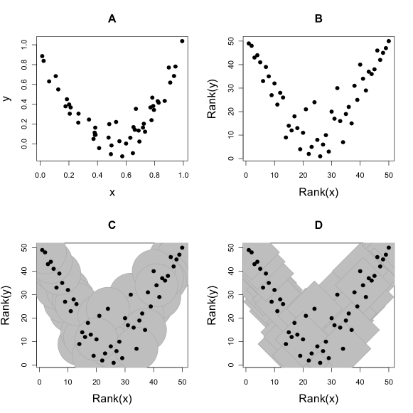
Figure 2: Illustration of RankCover for sample size $n=50$: A. Scatter plot of the two variables. B. Scatter plot on the rank scale C. Disks laid on the scatter plot on rank scale using Euclidian distance D. Disks laid on the scatter plot on rank scale using Manhattan distance.

2.2 The test statistic

The empirical estimate of $F$ can be obtained using the proportion of area covered by the disks. Acknowledging the discrete nature of the ranks, we consider only the $n\times n$ grid of possible rank pairs, $\{1,2,...,n\}\times\{1,2,...,n\}$, and whether each of these values on the grid is covered by at least one disk. Let $(x_{k},y_{k})$ denote the ranks of the $k$th sample pair, $k=1,2,...,n$.

Definition 2.1

Define $d(i,j,x_{k},y_{k})$ = distance between the point $(i,j)$ on the grid and $(x_{k},y_{k})$; $d_{ij}=\min_{k}d(i,j,x_{k},y_{k})$

Using this definition, a reasonable statistic for fixed $\delta$ is

$$\hat{F}(\delta)=\frac{1}{n^{2}}\sum_{i=1}^{n}\sum_{j=1}^{n}{I(d_{ij}\leq\delta)},$$

where $I(.)$ is the indicator function.

The choice of disk size $\delta$ is an important consideration which has not been fully addressed in the spatial statistics literature. Diggle (1983) suggested computing the entire empirical curve $\hat{F}(\delta)$ to develop a new summary statistic to compare against the null curve. However, this approach makes the procedure prohibitively computationally expensive, and we propose (See Supplementary Article for details) using a fixed $\delta=\sqrt{n}$ for Euclidean distance (Section 2.3), with slight modification under Manhattan distance. In addition, we modify the statistic to account for edge effects of the grid, using an $(n+\lceil\delta\rceil)\times(n+\lceil\delta\rceil)$ grid extending beyond the range of the scatterplot. Here $\lceil\delta\rceil$ is the smallest integer greater than or equal to $\delta$. Finally, our modified test statistic is

$$T(\delta)=\frac{1}{n^{2}}\sum_{i=1-\lceil\delta\rceil}^{n+\lceil\delta\rceil}\sum_{j=1-\lceil\delta\rceil}^{n+\lceil\delta\rceil}{I(d_{ij}\leq\delta)},$$ (2.1)

where the range of $\{i,j\}$ reflects the outer boundaries of a larger region to account for edge effects. The null distribution of $T$ depends entirely on $n$, so tables based on simulated null distibutions can be precomputed for various sample sizes (See Supplementary Article).

2.3 Choice of parameters and distance metric

For the distance metric $d$, we consider here both Euclidian and Manhattan distances, for which later simulations show similar performance (See Supplementary Article). However, the Manhattan distance has advantages in approximating tail areas (See Supplementary Article). Therefore we recommend its use and here present results using Manhattan distance.

3 Results

We applied the RankCover method using the Manhattan metric to simulated and real datasets, following setups similar to Simon and Tibshirani (2014), investigating dCor, HHG, and MIC as competing approaches. The simulation results indicate that RankCover and dCor have some complementary characteristics, and so we additionally propose a hybrid statistic using results from RankCover and dCor. The hybrid method uses the minimum $p$-value from RankCover and rank-based dCor as a new statistic. In addition to simulated data, we illustrate all the approaches on several real datasets.

Figure 3: Showing the scatter plots for different relationships between the pair of variables (low noise level)

3.1 Simulation results

Following the simulation procedure used in Simon and Tibshirani (2014), we have simulated pairs of variables with several canonical dependency relationships (Figure 3) and with varying noise levels. In each scenario, the $X$ values were simulated iid from a uniform distribution, while the noise distribution was Gaussian. However, the overall results were similar for other distributional forms (See Supplementary Article).

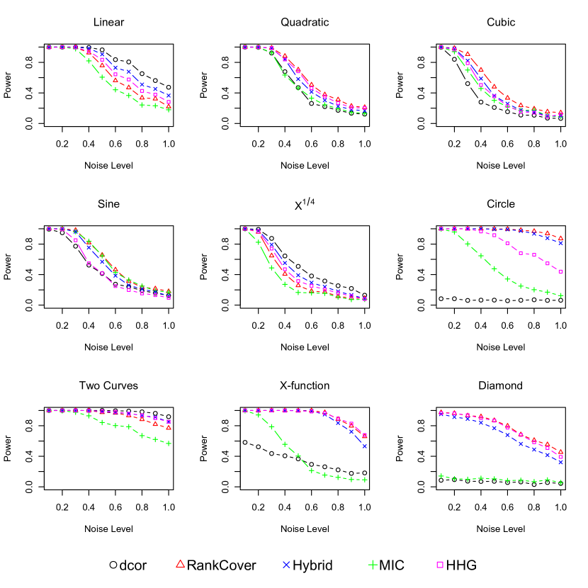
Figure 4: Showing the power of different methods (type-I $\alpha=0.05$ )against different relationships at varying noise levels.

Figure 4 shows the power for the methods for various relationships, with varying noise levels, for sample size $n=50$. Here the “noise level" is a scale quantity appropriate to each relationship form, following Simon and Tibshirani (2014) (See Supplementary Article). It is evident that RankCover performs better than MIC in all the situations we have considered. It is found to be more powerful than dCor and HHG in several cases while these methods are found to be more powerful in other cases. Even when dCor or HHG is more powerful, RankCover still has reasonable power to identify the association. Numerous illustrations provided in the supplementary article indicate that these observations hold true for varying sample sizes, levels of noise, and functional forms for the originating $X$ and noise distributions.

A careful look into the results indicate that dCor is more powerful than RankCover when the type of association is monotone. When the relationship is non-monotone, dCor is typically not as powerful. We attribute this behavior to the fact that dCor is less sensitive to non-monotone relationships for the reasons described earlier. We have also shown that with monotone relationships the Spearman’s rank correlation is as powerful as dCor (See Supplementary Article). Therefore, one might simply use Spearman’s rank correlation if there is prior knowledge that the relationship is monotone. On the other hand, RankCover is more sensitive to local clustering of points rather than trends. Thus, it is powerful against even non-monotone relationships like cubic, circular or the “X” relationship.

These observations motivate the use of a hybrid method utilizing both RankCover and dCor, as the two methods appear powerful in different situations. Formally, a new statistic is defined $s_{hybrid}={\rm min}(p_{dCor},p_{RankCover})$, where $p_{RankCover}$ is the $p$-value obtained by using RankCover, and $p_{dCor}$ is that using dCor on $(rank(x),rank(y))$. The $p$-value for the hybrid method is $p_{hybrid}=P(S_{hybrid}\leq s_{hybrid})$. As with RankCover, the $p$-value can be obtained by using pre-computed simulations. The hybrid method, as expected, is always less powerful than the most powerful statistic for each scenario, but seems to be robust against all forms of association investigated.

The HHG method also appears to be relatively robust. However, the ability of RankCover and the hybrid method to detect periodic relationships and non-functional relationships makes it very useful against such alternatives. The fact that RankCover is especially powerful against periodic relationships will be reinforced by the results in Section 3.2.3 and Section 3.2.4.

We summarize by emphasizing that RankCover and the hybrid method are powerful and robust in comparison to competing methods, and that these simulations cover a large range of relationships and noise levels. The broad conclusions are also not very sensitive to the marginal distributions of $X$ and the error distributions (See Supplementary Article).

3.2 Real data

3.2.1 Example 1: Eckerle4 data

We show data from a study of circular interference transmittance (Eckerle, 1979) from the NIST Statistical Reference Datasets for non-linear regression. The data were analyzed by Székely and Rizzo (2009) to illustrate dCor, and contain 35 observations on the predictor variable wavelength and the response variable transmittance.

Figure 5 shows the scatter plot of the predictor and the response along with the fitted curve (NIST StRD for non-linear regression) based on the model

$y=\frac{\beta_{1}}{\beta_{2}}exp\{\frac{(x-\beta_{3})^{2}}{2\beta_{2}^{2}}\}+\epsilon$,

where $\beta_{1},\beta_{2}>0,\beta_{3}\in\mathbb{R}$ and $\epsilon$ is random Gaussian noise.

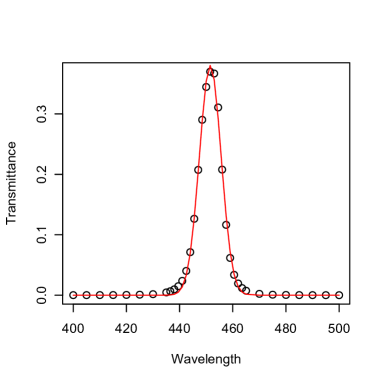
Figure 5: Showing the scatter plot and the fitted curve for the Eckerle4 dataset

From the plot, it is evident that there is a very strong non-linear relationship between the two variables. For dCor, $p=0.02072$, while MIC and HHG have $p$-values $<10^{-5}$. The RankCover method and the hybrid method are also highly significant, with $p<10^{-5}$.

3.2.2 Example 2: Aircraft data

We have explored the Saviotti aircraft data (Saviotti, 1996) which was also analyzed by Székely and Rizzo (2009). We consider the wing span (m) vs. speed (km/h) ($n=230$, Bowman and Azzalini (1997)). Figure 6 shows the scatter plot of the two variables, alongside non-parametric density estimate contours (log scale). It is clear from the plot that there is a non-linear relationship ( Pearson’s product moment correlation is a modest $0.0168$, $p$-value$=0.8001$), although the relationship is complicated and apparently not monotone.

Figure 6: Showing the scatter plot and the density estimate contours for the aircraft speed and wing span

All of the methods described here were significant at $\alpha=0.05$. The $p$-values for dCor, MIC, and HHG were 0.00013, 0.00004, and $<10^{-5}$, respectively. For RankCover the test was also significant with a $p=0.0008$, and for the hybrid method $p=0.0002$.

3.2.3 Example 3: ENSO data

The ENSO data ( also taken from the NIST Statistical Reference Datasets for non-linear regression) consists of monthly average atmospheric pressure differences between Easter Island and Darwin, Australia (Kahaner, Moler, Nash, and Forsythe, 1989), with 168 observations. There are 168 observations.The data form a time series, and has different cyclical components which were modeled (NIST StRD for non-linear regression) by the proposed model

$y=\beta_{1}+\beta_{2}cos(\frac{2\pi x}{12})+\beta_{3}sin(\frac{2\pi x}{12})+\beta_{5}cos(\frac{2\pi x}{\beta_{4}})+\beta_{6}sin(\frac{2\pi x}{\beta_{4}})+\beta_{8}cos(\frac{2\pi x}{\beta_{7}})+\beta_{9}sin(\frac{2\pi x}{\beta_{7}})+\epsilon$,

where $\beta_{1},\beta_{2},...,\beta_{9}\in\mathbb{R}$ and $\epsilon$ is random Gaussian noise.

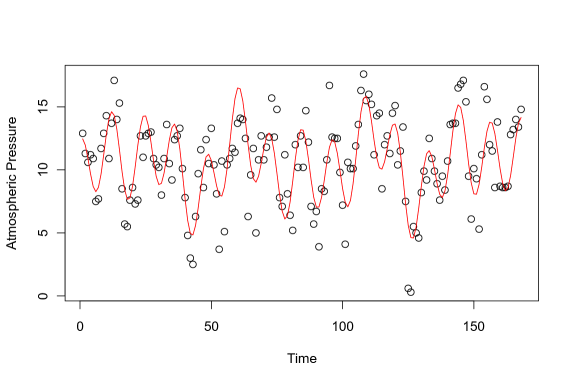
Figure 7: Showing the scatter plot and the fitted curve for the ENSO dataset

Figure 7 shows the scatter plot of the data along with the fitted curve. The cyclical fluctuations are evident, but no linear trend is observed. Thus, the Pearsonian correlation (0.0843) fails to capture the pattern. However a simple serial correlation with lag 1 (0.6102) reveals the association. With 100,000 simulations, the RankCover test is significant with $p$-value 0.00032. The hybrid test and MIC test are also significant with $p$-values 0.00064 and 0.00027 respectively. However dCor and HHG fail to detect significant association ($p$-values 0.13521 and 0.07617, respectively).

3.2.4 Example 4: Yeast data

In this example, we analyze a yeast cell cycle gene expression dataset with 6223 genes Spellman et al. (1998). The experiment was designed to identify genes with activity varying throughout the cell cycle (Spellman, Sherlock, Zhang, Iyer, Anders, Eisen, Brown, Botstein, and Futcher, 1998), and thus transcript levels would be expected to oscillate. This data has been analyzed by many researchers, including Reshef, Reshef, Finucane, Grossman, McVean, Turnbaugh, Lander, Mitzenmacher, and Sabeti (2011), who used it to verifying the ability of MIC to detect oscillating patterns. We have run dCor, MIC, HHG, RankCover and the hybrid methods of test on the data and used the Benjamini-Hochberg method to control the false discovery rate.

We have listed the genes identified by different methods after controlling the false discovery rate (FDR) at the 5% level and compared them with the list of genes identified by Spellman, Sherlock, Zhang, Iyer, Anders, Eisen, Brown, Botstein, and Futcher (1998). Of all the genes identified by Spellman et al. (1998), RankCover found 16% to be significant, while dCor, MIC and HHG found only 6%, 2% and 8% respectively. The hybrid method could identify 12% of those genes. Instead controlling the FDR at 25%, the figures for HHG, dCor, MIC, RankCover and the hybrid method become 39%, 23%, 18%, 57% and 47% respectively. These figures differ slightly from those reported in Reshef et al. (2011), due to the difference in the procedure of handling the missing data (See Supplementary Article for details).

For these data, RankCover is clearly successful at identifying oscillating patterns expected for the experiment. This is also clear from Figure 8 (panel A, B and C) which compares the FDR adjusted $q$-values of our RankCover test with those of dCor, MIC and HHG on a logarithmic scale. Most of the genes in Spellman’s list which are identified by dCor, MIC or HHG are also identified by RankCover, but RankCover identified more genes than the other methods. Figure 8 (panels D-I) shows some of the genes that are found significant by RankCover at 5% level, but not found significant by at least one of the other three methods. PDR5 was found significant by MIC, HHG and RankCover, but not by dCor. On the other hand MIC could not identify FET3, which was identified by dCor, HHG and RankCover. The other four genes shown in Figure 8 are found significant by RankCover but not by dCor, MIC or HHG. Note that all the six genes are found to be significant by the hybrid method.

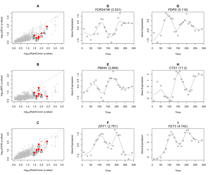
Figure 8: A. The plot comparing the FDR adjusted $q$-values of the test using RankCover and that using dCor for the genes in Spellman’s list in a log scale. It is evident that most of the genes in Spellman’s list have a smaller $q$-value when RankCover test is used. B. A similar plot comparing the $q$-values of RankCover and MIC. C. A similar plot comparing the $q$-values of RankCover and HHG. D-I. Examples of genes in the Spellman’s list that were identified by RankCover, but not by at least one of dCor, MIC or HHG. The values in parentheses are the Spellman scores for the genes.

4 Summary

Our RankCover testing procedure serves as a simple and powerful method to test for general association between a pair of variables. The method is applicable to the problem of testing general association irrespective of the marginal distributions of the (continuous) variables. Use of the rank scale also allows a pre-computed null distribution for the statistic, avoiding the need for actual permutation. This, along with the introduction of the idea of using a single disk size makes the procedure computationally feasible. The testing procedure has been shown to be powerful in simulated datasets even with a small sample size. A variety of real datasets, ranging from studies of cell cycle effects in gene expression to studies involving circular interference transmittance show that the approach provides useful and interpretable results.

Although dCor is theoretically motivated by consideration of characteristic functions, in practice it suffers for non-monotone relationships. Our RankCover procedure is generally powerful and robust, and is more powerful than MIC, dCor and HHG for a number of scenarios. RankCover may be especially useful to detect oscillating relationships, keeping in mind that such relationships need not be periodic and the amplitudes may vary. A hybrid of RankCover and dCor is proposed, which is shown to be highly robust against many forms of associations.

With the rapid rise of large datasets in today’s scientific community, RankCover provides a useful tool to detect general association. The approach is both sensitive and relatively powerful, even with small samples, against various and general forms of association.

References

- Albert et al. (2001) Albert, P. S., D. Ratnasinghe, J. Tangrea, and S. Wacholder (2001). Limitations of the case-only design for identifying gene-environment interactions. American Journal of Epidemiology 154(8), 687–693.
- Bowman and Azzalini (1997) Bowman, A. W. and A. Azzalini (1997). Applied Smoothing Techniques for Data Analysis: The Kernel Approach with S-Plus Illustrations: The Kernel Approach with S-Plus Illustrations. Oxford University Press.
- Clark and Evans (1954) Clark, P. J. and F. C. Evans (1954). Distance to nearest neighbor as a measure of spatial relationships in populations. Ecology, 445–453.
- Cuzick (1985) Cuzick, J. (1985). A wilcoxon-type test for trend. Statistics in medicine 4(4), 543–547.
- de Siqueira Santos et al. (2013) de Siqueira Santos, S., D. Y. Takahashi, A. Nakata, and A. Fujita (2013). A comparative study of statistical methods used to identify dependencies between gene expression signals. Briefings in bioinformatics, bbt051.
- Diggle (1983) Diggle, P. J. (1983). Statistical analysis of spatial point patterns. Academic Press London.
- Eckerle (1979) Eckerle, K. (1979). Circular interference transmittance study. National Institute of Standards and Technology (NIST), US Department of Commerce, USA.
- Hamed and Ramachandra Rao (1998) Hamed, K. H. and A. Ramachandra Rao (1998). A modified mann-kendall trend test for autocorrelated data. Journal of Hydrology 204(1), 182–196.
- Heller et al. (2013) Heller, R., Y. Heller, and M. Gorfine (2013). A consistent multivariate test of association based on ranks of distances. Biometrika 100(2), 503–510.
- Holgate (1965a) Holgate, P. (1965a). Some new tests of randomness. The Journal of Ecology, 261–266.
- Holgate (1965b) Holgate, P. (1965b). Tests of randomness based on distance methods. Biometrika 52(3-4), 345–353.
- Kahaner et al. (1989) Kahaner, D., C. B. Moler, S. Nash, and G. E. Forsythe (1989). Numerical methods and software. Prentice-Hall Englewood Cliffs, NJ.
- Kendall (1975) Kendall, M. (1975). Rank correlation methods. Griffin, London.
- Mann (1945) Mann, H. B. (1945). Non-parametric test against trend. Econometrika 13, 245–259.
- Puri and Sen (1971) Puri, M. L. and P. K. Sen (1971). Nonparametric methods in multivariate analysis.
- Reshef et al. (2011) Reshef, D. N., Y. A. Reshef, H. K. Finucane, S. R. Grossman, G. McVean, P. J. Turnbaugh, E. S. Lander, M. Mitzenmacher, and P. C. Sabeti (2011). Detecting novel associations in large data sets. Science 334(6062), 1518–1524.
- Ripley (1979) Ripley, B. (1979). Tests of ‘randomness’ for spatial point patterns. Journal of the Royal Statistical Society. Series B (Methodological), 368–374.
- Saviotti (1996) Saviotti, P. (1996). Technological evolution, variety, and the economy. E. Elgar.
- Simon and Tibshirani (2014) Simon, N. and R. Tibshirani (2014). Comment on “detecting novel associations in large data sets" by reshef et al, science dec 16, 2011. arXiv preprint arXiv:1401.7645.
- Smith (2004) Smith, T. E. (2004). A scale-sensitive test of attraction and repulsion between spatial point patterns. Geographical analysis 36(4), 315–331.
- Spellman et al. (1998) Spellman, P. T., G. Sherlock, M. Q. Zhang, V. R. Iyer, K. Anders, M. B. Eisen, P. O. Brown, D. Botstein, and B. Futcher (1998). Comprehensive identification of cell cycle–regulated genes of the yeast saccharomyces cerevisiae by microarray hybridization. Molecular biology of the cell 9(12), 3273–3297.
- Székely and Rizzo (2009) Székely, G. J. and M. L. Rizzo (2009). Brownian distance covariance. The annals of applied statistics 3(4), 1236–1265.
- Székely et al. (2007) Székely, G. J., M. L. Rizzo, and N. K. Bakirov (2007). Measuring and testing dependence by correlation of distances. The Annals of Statistics 35(6), 2769–2794.
- Wilks (1935) Wilks, S. (1935). On the independence of k sets of normally distributed statistical variables. Econometrica, Journal of the Econometric Society, 309–326.