John Ellis^a, Marcos A. G. García^b, Dimitri V. Nanopoulos^c
and
Keith A. Olive^b

^aTheoretical Particle Physics and Cosmology Group, Department of Physics, King’s College London, London WC2R 2LS, United Kingdom;
Theory Division, CERN, CH-1211 Geneva 23, Switzerland
^bWilliam I. Fine Theoretical Physics Institute, School of Physics and Astronomy,
University of Minnesota, Minneapolis, MN 55455, USA
^cGeorge P. and Cynthia W. Mitchell Institute for Fundamental Physics and Astronomy, Texas A&M University, College Station, TX 77843, USA;
Astroparticle Physics Group, Houston Advanced Research Center (HARC),
Mitchell Campus, Woodlands, TX 77381, USA;
Academy of Athens, Division of Natural Sciences, Athens 10679, Greece

ABSTRACT

Since the building-blocks of supersymmetric models include chiral superfields containing pairs of effective scalar fields, a two-field approach is particularly appropriate for models of inflation based on supergravity. In this paper, we generalize the two-field analysis of the inflationary power spectrum to supergravity models with arbitrary Kähler potential. We show how two-field effects in the context of no-scale supergravity can alter the model predictions for the scalar spectral index $n_{s}$ and the tensor-to-scalar ratio $r$, yielding results that interpolate between the Planck-friendly Starobinsky model and BICEP2-friendly predictions. In particular, we show that two-field effects in a chaotic no-scale inflation model with a quadratic potential are capable of reducing $r$ to very small values $\ll 0.1$. We also calculate the non-Gaussianity measure $f_{\rm NL}$, finding that is well below the current experimental sensitivity.

September 2014

1 Introduction

The recent results from the Planck satellite [1] and the BICEP2 experiment [2] have inaugurated a new era in the confrontation of inflationary models with observation. Planck has provided whole-sky measurements of the cosmic microwave background (CMB) with unparalleled precision down to small angular scales, confirming the previous indications from WMAP [3] that the scalar index $n_{s}<1$ and refining previous upper limits on the tensor-to-scalar ratio $r$. Moreover, Planck has provided stringent upper limits on many possible non-Gaussian features in the CMB [1]. More recently, BICEP2 has detected B-mode polarization in the CMB [2], and triggered a raging debate on its interpretation [4, 5]. In particular, how much of it is due to foreground galactic dust, and how much may be primordial? A recent Planck analysis [6] indicates that the BICEP2 signal may well be dominated by foreground dust, in which case values of $r\lower 3.01385pt\hbox{$\;\stackrel{{\scriptstyle\textstyle<}}{{\sim}}\;$}0.1$ would be favoured [7].

The Planck results [1] dampened interest in multi-field models that could give large values of $f_{\rm NL}$ and stimulated interest in models that predicted small values of $r$, such as the Starobinsky model based on a $R+R^{2}$ modification of Einstein gravity [8, 9, 10]. There has also been renewed interest in the construction of models that reduce, at least approximately, to the Starobinsky model, such as Higgs inflation [11]. In this connection, attention was drawn to a class of supergravity models that reduce to the $R+R^{2}$ model and reproduce its predictions for $r$ and $n_{s}$, and there has subsequently been much interest in exploring this class of models [12, 13, 14, 15, 16, 17, 18, 19, 20, 21, 22, 23].

An important aspect of these models is that, since generic supersymmetric models use chiral supermultiplets as building-blocks, and since each chiral supermultiplet contains two real fields, generic supersymmetric models of inflation, including supergravity models, contain an even number of scalar fields . For this reason, it is appropriate to use a multi-field approach to analyze the predictions of supersymmetric models of inflation. This has been done, for example, in the context of a Wess-Zumino model of inflation [24], and its importance for supergravity models of inflation has been stressed in [25], as was taken into account in the published version of [26].

In supergravity models, and in two-field models in general, the evolution of the inflaton may take a non-trivial path in field space depending on how the two fields are coupled both in the potential and in their kinetic terms. The simplest example of such a non-trivial path occurs when the two fields have different masses. The cosmological evolution starts down the path of steepest decent (in the direction of the heavier field), and then turns down the lighter direction towards the global minimum. This case has been well studied [27, 28, 29], and it has been shown that isocurvature fluctuations perpendicular to the direction of the motion of the scalar field eventually source adiabatic perturbations as the field evolves towards the global minimum. The extra source of adiabatic scalar perturbations then tends to suppress the tensor-to-scalar ratio, $r$.

We consider the natural framework for formulating models of inflation to be supersymmetry [30, 31, 32, 33], specifically local supersymmetry, i.e., supergravity [34]. Whereas the Planck limits on $r$ favour inflationary models resembling the Starobinsky model [8, 9, 10], the BICEP2 results point back to simple models of quadratic chaotic inflation [35]. The first attempt at a chaotic inflation model in the context of supergravity was made in [33]. In view of the eta problem in supergravity [36], many of the simplest models employ a shift symmetry in the Kähler potential [37, 38]. This may be realized in the context where the sneutrino plays the role of the inflaton [39], or in relation to moduli stabilization [40]. However, no-scale supergravity [41] offers an alternative solution to address the eta problem, and has many other attractive features, including its appearance in generic string compactifications [42]. Here we are interested in inflationary models [43, 44, 45, 46, 12, 13, 17, 47, 26] based on no-scale supergravity .

In view of the current uncertainty in the value or $r$, which may take any value between 0 and 0.1 or more, inflationary model-builders are enjoying a field-day until the uncertainty is reduced. One possibility is to commit strongly to some particular model of inflation and its predictions. Another approach is to formulate more general frameworks that can accommodate a wider range of predictions compatible with the present observational range of $r$. The latter was the point of view taken in [26], where it was shown how a class of simple no-scale supergravity models could interpolate between the prediction $r\sim 0.15$ of chaotic inflation in a quadratic potential and the prediction $r\sim 0.003$ of the Starobinsky model .

The value of $r$ in the model in [26] was varied by adjusting the angle in the complex plane of a valley in the effective potential for the complex modulus field $T$ of the simplest no-scale supergravity model that provides the inflaton. The complications of two-field inflation [25] were avoided in this model by requiring the walls of the potential valley to be very steep, effectively constraining the inflaton trajectory to the analogue of a narrow “bobsleigh track”.

In this paper we take a different approach. Working in the same no-scale supergravity framework, we vary the parameter controlling the width of the potential valley. In this way, we are able to dial up the importance of the two-field effects. As we show, they have relatively little effect on the value of $n_{s}$ in this model, which is almost always compatible with the experimental value $n_{s}\simeq 0.960\pm 0.008$. On the other hand, two-field effects may enhance the magnitude of the scalar perturbations above the value expected naively from a single-field analysis, thereby suppressing the tensor-to-scalar ratio $r$. This provides an independent way to interpolate between the limits of chaotic quadratic inflation and Starobinsky-like models that, as we verify, does not lead to large non-Gaussianities.

The layout of this paper is as follows. Section 2 first reviews the class of no-scale supergravity models we consider, and then presents the (modest extension of) the standard two-field formalism required to analyze this class of models. Section 3 then applies this formalism to the no-scale supergravity model of interest, focusing on initial conditions with ${\cal R}e~{}T=0$, which would seem in a single-field treatment to yield large values of $r$. We show explicitly that, as the width of the potential valley increases, the trajectory of the inflaton veers into the real direction: ${\cal R}e~{}T\gg{\cal I}m~{}T$ and $r$ assumes values closer to the Starobinsky value. Section 4 describes our calculation of the non-Gaussianity parameter $f_{\rm NL}$, which we find to be always small: $f_{\rm NL}\lower 3.01385pt\hbox{$\;\stackrel{{\scriptstyle\textstyle<}}{{\sim}}\;$}0.03$. Finally, Section 5 summarizes our conclusions and prospects.

2 Model and Formalism

2.1 Specification of the Model

As discussed in [26], the Kähler potential of the minimal no-scale supergravity model has the form [41]

$$K\;=\;-3\ln(T+\bar{T})+\dots\,,$$ (1)

where the dots represent corrections to the Kähler potential due to perturbative or non-perturbative effects, additional matter fields $\phi$, etc. . As already mentioned, one of the reasons for our interest in no-scale supergravity is that it is the natural framework for the low-energy effective field theory in a generic string compactification [42], where $T$ is identified as a complex modulus field. In a no-scale supergravity model with an underlying SU$(2,1)$/SU$(2)$ $\times$ U(1) symmetry, the Kälhler potential could be written as

$$K\;=\;-3\ln\left(T+\bar{T}-\frac{\phi\phi^{*}}{3}\right)\,,$$ (2)

If we identify $T$ as the chiral (two-component) inflaton superfield, and we assume the following superpotential [49] for our no-scale supergravity model of inflation:

$$W\;=\;\sqrt{\frac{3}{4}}\,\frac{m}{a}\phi(T-a)\,.$$ (3)

Starobinsky-type inflation would occur if initial conditions placed $T$ along the real axis [14, 13]. Although the potential is quadratic along the imaginary $T$ axis [50], the evolution of the field moves it to the real axis, leading again to Starobinsky-like inflation unless $T$ is stabilized along its imaginary direction using a higher order term such as $(T+T^{*})^{n}$ in the Kähler potential [51, 47, 50]. In addition this type of model is not easily generalized to allow inflation “off-axis”.

In typical orbifold string compactifications with three moduli that are fixed by some unspecified mechanism at a high scale to be proportional, the Kähler potential may be written in the following form [52]:

$$K\;=\;-3\ln(T+\bar{T})+\frac{|\phi|^{2}}{(T+\bar{T})^{3}}\,,$$ (4)

up to irrelevant constants, where we consider a single matter field $\phi$ with modular weight $3$. Here, as in [26], we use the superpotential given in Eq. (3). As discussed in [26], the matter field $\phi$ is constrained by the exponential factor $e^{K}$:

$$V\;\propto\;e^{|\phi|^{2}/(T+\bar{T})^{3}}\;\simeq\;e^{(2a)^{-3}|\phi|^{2}}\,.$$ (5)

We assume that $a=1/2$, in which case $\phi\to 0$ rapidly at the start of inflation, and the scalar potential takes the simple form

$$V=\frac{3m^{2}}{4a^{2}}|T-a|^{2}\,.$$ (6)

We write $T$ in terms of two real fields $\rho$ and $\alpha$ that parameterize its real and imaginary components, respectively:

$$T\;=\;a\left(e^{-\sqrt{\frac{2}{3}}\rho}+i\sqrt{\frac{2}{3}}\,\alpha\right)\,,$$ (7)

with the following effective Lagrangian:

$$\mathcal{L}\;=\;\frac{1}{2}\partial_{\mu}\rho\partial^{\mu}\rho+\frac{1}{2}e^{2\sqrt{\frac{2}{3}}\rho}\partial_{\mu}\alpha\partial^{\mu}\alpha-\frac{3}{4}m^{2}\left(1-e^{-\sqrt{\frac{2}{3}}\rho}\right)^{2}-\frac{1}{2}m^{2}\alpha^{2}\,.$$ (8)

Moreover, the coupling between $\rho$ and $\alpha$ through the kinetic term in (8) yields a coupling between the curvature and isocurvature perturbations, resulting in an enhancement of the curvature modes at super-horizon scales whose calculation requires a two-field analysis.

2.2 Two-Field Formalism

Multi-field inflation has been discussed extensively in the literature (see, for example, [53, 27] for multi-field inflation with canonical kinetic terms, [54, 55, 28] for examples with particular non-canonical kinetic terms, and [56] for a discussion of more general kinetic terms). Here we present an additional review where we emphasize aspects of the generic multi-field formalism relevant to inflationary models arising in $\mathcal{N}=1$ supergravity, presenting the equations in a form that allows their immediate application.

Disregarding gauge interactions, the scalar $\mathcal{N}=1$ supergravity action for the scalar sector can be written as

$$S\;=\;\int d^{4}x\,\sqrt{-g}\left[K_{I\bar{J}}\partial_{\mu}\Phi^{I}\partial^{\mu}\bar{\Phi}^{\bar{J}}-V(\boldsymbol{\Phi})\right]\,,$$ (9)

with the scalar potential

$$V\;=\;e^{K}(K^{\bar{I}J}D_{J}W\bar{D}_{\bar{I}}\bar{W}-3|W|)\,.$$ (10)

Here $\{\Phi_{I}\}:I=1,\dots,n$ denote the $n$ complex components of the chiral superfields, $D_{I}W=\partial_{I}W+K_{I}W$ and $K_{I}$ is the derivative of the field labeled by $I$ . Equivalently, the action (9) can be rewritten in terms of the real and imaginary components of these complex fields:

$$\Phi^{I}\;=\;\frac{1}{\sqrt{2}}(\chi^{I}+i\zeta^{I})\,.$$ (11)

Substituting (11) into the scalar potential (10), the action (9) takes the form

$$S =\int d^{4}x\,\sqrt{-g}\Bigg{[}\frac{1}{2}\,\left(\partial_{\mu}\chi^{I},\partial_{\mu}\zeta^{I}\right)\left(\begin{matrix}K_{I\bar{J}}^{\mathcal{R}}&K_{I\bar{J}}^{\mathcal{I}}\\ -K_{I\bar{J}}^{\mathcal{I}}&K_{I\bar{J}}^{\mathcal{R}}\end{matrix}\right)\left(\begin{matrix}\partial^{\mu}\chi^{J}\\ \partial^{\mu}\zeta^{J}\end{matrix}\right)-V(\boldsymbol{\chi},\boldsymbol{\zeta})\Bigg{]}$$

$$\equiv\int d^{4}x\,\sqrt{-g}\left[\frac{1}{2}G_{ij}\partial_{\mu}\phi^{i}\partial^{\mu}\phi^{j}-V(\boldsymbol{\phi})\right]\,,$$ (12)

where $i=1,\dots,2n$, and $K_{I\bar{J}}^{\mathcal{R,I}}$ denote the real and imaginary parts of $K_{I\bar{J}}$. It can readily be verified that the real field metric $G_{ij}$ is symmetric. Equation (2.2) will be the starting point for our review of multi-field inflation.

Assuming a spatially flat Friedmann-Robertson-Walker geometry, with the metric

$$ds^{2}\;=\;dt^{2}-a(t)^{2}\,d\bf{x}^{2}\ ,$$ (13)

the classical (background) equations of motion for the spatially uniform real scalar fields and the scale factor correspond to

$$\ddot{\phi}^{i}+\Gamma^{i}_{jk}\dot{\phi}^{j}\dot{\phi}^{k}+3H\dot{\phi}^{i}+G^{ij}V_{,j}\;=\;0\,,$$ (14)

where

$$H^{2}\;=\;\frac{1}{3}\left[\frac{1}{2}G_{ij}\dot{\phi}^{i}\dot{\phi}^{j}+V\right]\,,$$ (15)

and

$$\dot{H}\;=\;-\frac{1}{2}G_{ij}\dot{\phi}^{i}\dot{\phi}^{j}\,.$$ (16)

Here $H\equiv\dot{a}/a$ denotes the Hubble parameter, $G^{ij}$ is the inverse field metric, and $\Gamma^{i}_{jk}$ is the connection in field space.

Next, we generalize the treatment of linear perturbations in [28] in a way applicable to the model defined by the action (2.2). The Newtonian (or longitudinal) gauge for the gravitational perturbations is a convenient gauge choice, since the anisotropic stress for the scalar fields vanishes in the linear approximation. The perturbed metric then takes the form

$$ds^{2}\;=\;(1+2\Psi)dt^{2}-a^{2}(1-2\Psi)d{\bf x}^{2}\,.$$ (17)

Decomposing the fields into the uniform background and the space-time-dependent perturbation

$$\phi^{i}(t,{\bf x})\;=\;\phi^{i}(t)+\delta\phi^{i}(t,{\bf x})\,,$$ (18)

the resulting perturbed equations of motion for the fields in Fourier space read

$$\ddot{\delta\phi^{i}}+2\Gamma^{i}_{jk}\dot{\phi}^{j}\dot{\delta\phi^{k}}+3H\dot{\delta\phi^{i}}+\frac{k^{2}}{a^{2}}\delta\phi^{i}+\left[(G^{ij}V_{,j})_{,k}+\Gamma^{i}_{jl,k}\dot{\phi}^{j}\dot{\phi}^{l}\right]\delta\phi^{k}\;=\;4\dot{\phi}^{i}\dot{\Psi}-2G^{ik}V_{,k}\Psi$$ (19)

while Einstein’s equations lead to

$$\ddot{\Psi}+4H\dot{\Psi}+(\dot{H}+3H^{2})\Psi\;=\;\frac{1}{2}\left[G_{ij}\dot{\phi}^{i}\dot{\delta\phi^{j}}+\frac{1}{2}G_{ij,k}\dot{\phi}^{i}\dot{\phi}^{j}\delta\phi^{k}-V_{,k}\delta\phi^{k}\right]\,,$$ (20)

$$3H(\dot{\Psi}+H\Psi)+\dot{H}\Psi+\frac{k^{2}}{a^{2}}\Psi\;=\;-\frac{1}{2}\left[G_{ij}\dot{\phi}^{i}\dot{\delta\phi^{j}}+\frac{1}{2}G_{ij,k}\dot{\phi}^{i}\dot{\phi}^{j}\delta\phi^{k}+V_{,k}\delta\phi^{k}\right]\,,$$ (21)

$$H\Psi+\dot{\Psi}\;=\;\frac{1}{2}G_{ij}\dot{\phi}\delta\phi^{j}\,.$$ (22)

In terms of the gauge-invariant Mukhanov-Sasaki variables,

$$Q^{i}\;\equiv\;\delta\phi^{i}+\frac{\dot{\phi}^{i}}{H}\Psi\,,$$ (23)

the multi-field perturbation equations (19)-(22) reduce to

$$\ddot{Q}^{i}+2\Gamma^{i}_{jk}\dot{\phi}^{j}\dot{Q}^{k}+3H\dot{Q}^{i}+\frac{k^{2}}{a^{2}}Q^{i}+C^{i}_{k}Q^{k}\;=\;0\,,$$ (24)

where the coefficients $C^{i}_{k}$ are defined as

$$C^{i}_{k}\;\equiv 3G_{jk}\dot{\phi}^{i}\dot{\phi}^{j}-\frac{1}{2H^{2}}G_{jk}G_{lm}\dot{\phi}^{i}\dot{\phi}^{j}\dot{\phi}^{l}\dot{\phi}^{m}+\Gamma^{i}_{jl,k}\dot{\phi}^{j}\dot{\phi}^{l}+G^{ij}G_{lk}\frac{\dot{\phi}^{l}}{H}V_{,j}+\frac{\dot{\phi}^{i}}{H}V_{,k}$$ (25)

$$\ +(G^{ij}V_{,j})_{,k}\ .$$

The equations (24) form a closed system for describing the gauge-invariant perturbations $Q^{i}$. These equations are in general coupled and do not allow an immediate interpretation of the perturbations in terms of observables. Instead, it is customary to introduce a kinematical basis in which the corresponding components of the perturbations can be related directly to the curvature and isocurvature perturbations, which in turn lead to the observable amplitudes and power spectra.

The transition to the kinematical basis in the general multi-field scenario is discussed in [58]. Here we specialize to the two-field scenario, $i=1,2$. In this case, the kinematical basis consists of the instantaneous directions parallel and orthogonal to the background trajectory in field space. The speed in field space is conventionally denoted by $\dot{\sigma}$, where

$$\dot{\sigma}^{2}\;=\;G_{ij}\dot{\phi}^{i}\dot{\phi}^{j}\,,$$ (26)

The parallel and orthogonal directions to the background trajectory can be parametrized by the unit vectors

$$e_{\sigma}^{i}\equiv e_{\parallel}^{i}\;=\;\frac{\dot{\phi}^{i}}{\dot{\sigma}}\ ,\qquad e_{s}^{i}\equiv e_{\perp}^{i}\;=\;\tilde{G}^{i}_{j}\frac{\dot{\phi}^{j}}{\dot{\sigma}}\,,$$ (27)

where we have defined

$$\tilde{G}^{i}_{j}\;\equiv\;\frac{\epsilon^{ik}G_{kj}}{\sqrt{G}}\,,$$ (28)

with $\epsilon^{12}=1$. In this new basis, we introduce the adiabatic and isocurvature perturbations

$$\delta\sigma\;=\;G_{ij}e^{i}_{\sigma}\delta\phi^{j}\ ,\qquad\delta s\;=\;G_{ij}e^{i}_{s}\delta\phi^{j}\$$ (29)

and the directional derivatives

$$V_{\sigma}\;=\;e_{\sigma}^{i}V_{,i}\ ,\ \ V_{s}\;=\;e_{s}^{i}V_{,i}\ ,\ \ V_{\sigma\sigma}\;=\;e_{\sigma}^{i}e_{\sigma}^{j}V_{,ij}\ ,\ \ V_{\sigma s}\;=\;e_{\sigma}^{i}e_{s}^{j}V_{,ij}\ ,\ \ V_{ss}\;=\;e_{s}^{i}e_{s}^{j}V_{,ij}\,.$$ (30)

The background equations can now be written in this basis. The background isocurvature is constant, $\dot{s}\equiv G_{ij}e^{i}_{s}\dot{\phi}^{j}=0$, while the adiabatic homogeneous equation of motion corresponds to

$$\ddot{\sigma}+3H\dot{\sigma}+V_{\sigma}\;=\;0\,.$$ (31)

In turn, the equations of motion for the gauge-invariant perturbations

$$Q_{\sigma}\;=\;G_{ij}e^{i}_{\sigma}Q^{j}\ ,\qquad Q_{s}\;=\;G_{ij}e^{i}_{s}Q^{j}\ ,$$ (32)

correspond to

$$\ddot{Q}_{\sigma}+3H\dot{Q}_{\sigma}+2\frac{V_{s}}{\dot{\sigma}}\dot{Q}_{s}+\left(\frac{k^{2}}{a^{2}}+C_{\sigma\sigma}\right)Q_{\sigma}+C_{\sigma s}Q_{s} =\;0,$$ (33)

$$\ddot{Q}_{s}+3H\dot{Q}_{s}-2\frac{V_{s}}{\dot{\sigma}}\dot{Q}_{\sigma}+\left(\frac{k^{2}}{a^{2}}+C_{ss}\right)Q_{s}+C_{s\sigma}Q_{\sigma} =\;0\,,$$ (34)

where the background-dependent coefficients are

$$C_{\sigma\sigma} =\;V_{\sigma\sigma}-\left(\frac{V_{s}}{\dot{\sigma}}\right)^{2}+\frac{2\dot{\sigma}}{H}V_{\sigma}+3\dot{\sigma}^{2}-\frac{\dot{\sigma}^{4}}{2H^{2}}+\Gamma^{l}_{ik}G_{lj}\dot{\phi}^{i}\dot{\phi}^{j}\dot{\phi}^{k}\frac{V_{\sigma}}{\dot{\sigma}^{3}}+\epsilon_{il}\Gamma^{l}_{jk}\dot{\phi}^{i}\dot{\phi}^{j}\dot{\phi}^{k}\frac{V_{s}}{\dot{\sigma}^{3}}\,,$$ (35)

$$C_{\sigma s} =\;6H\frac{V_{s}}{\dot{\sigma}}+2\frac{V_{s}V_{\sigma}}{\dot{\sigma}^{2}}+2V_{\sigma s}+\frac{\dot{\sigma}V_{s}}{H}-2\tilde{G}^{l}_{i}G_{mk}\Gamma^{m}_{lj}\dot{\phi}^{i}\dot{\phi}^{j}\dot{\phi}^{k}\frac{V_{\sigma}}{\dot{\sigma}^{3}}$$

$$\quad-2\tilde{G}^{m}_{i}\tilde{G}^{l}_{j}G_{nl}\Gamma^{n}_{km}\dot{\phi}^{i}\dot{\phi}^{j}\dot{\phi}^{k}\frac{V_{s}}{\dot{\sigma}^{3}}\,,$$ (36)

$$C_{s\sigma} =\;-6H\frac{V_{s}}{\dot{\sigma}}-2\frac{V_{s}V_{\sigma}}{\dot{\sigma}^{2}}+\frac{\dot{\sigma}V_{s}}{H}\,,$$ (37)

$$C_{ss} =\;V_{ss}-\left(\frac{V_{s}}{\dot{\sigma}}\right)^{2}-\tilde{G}^{l}_{j}\tilde{G}^{m}_{k}G_{in}\Gamma^{n}_{lm}\dot{\phi}^{i}\dot{\phi}^{j}\dot{\phi}^{k}\frac{V_{\sigma}}{\dot{\sigma}^{3}}+\tilde{G}^{l}_{k}G_{jm}\Gamma^{m}_{il}\dot{\phi}^{i}\dot{\phi}^{j}\dot{\phi}^{k}\frac{V_{s}}{\dot{\sigma}^{3}}$$

$$\quad-\frac{1}{2}\left(\tilde{G}^{k}_{i}\tilde{G}^{mj}G_{ml}\Gamma^{l}_{kj}+\tilde{G}^{k}_{i}\Gamma^{l}_{kl}\right)\dot{\phi}^{i}\frac{V_{s}}{\dot{\sigma}}+\frac{1}{2}R\dot{\sigma}^{2}\ .$$ (38)

Here $R$ denotes the curvature scalar, $\epsilon_{12}=\sqrt{G}\epsilon^{12}$, and $\tilde{G}^{ij}=G^{-1}\epsilon^{ik}\epsilon^{jl}G_{kl}$. The adiabatic perturbation $Q_{\sigma}$ is related to the comoving curvature perturbation as:

$$\mathcal{R}\;=\;\frac{H}{\dot{\sigma}}Q_{\sigma}\,.$$ (39)

The isocurvature perturbation in turn defines the entropy perturbation,

$$\mathcal{S}\;=\;\frac{H}{\dot{\sigma}}Q_{s}\,.$$ (40)

At the start of inflation, deep inside the Hubble radius, the adiabatic and entropy fluctuations are initially statistically independent, and can be approximated by the corresponding Minkowski vacuum state:

$$Q_{\sigma}(\tau_{i})\;=\;\frac{e^{-ik\tau_{i}}}{a(\tau_{i})\sqrt{2k}}\xi_{\sigma}(k)\ ,\qquad Q_{s}(\tau_{i})\;=\;\frac{e^{-ik\tau_{i}}}{a(\tau_{i})\sqrt{2k}}\xi_{s}(k)\,,$$ (41)

where $d\tau\equiv dt/a$ is the conformal time, and $\xi_{I}:I=\sigma,s$ are independent Gaussian random variables satisfying

$$\langle\xi_{I}(k)\rangle\;=\;0\ ,\quad\langle\xi_{I}(k),\bar{\xi}_{J}(k^{\prime})\rangle=\delta_{IJ}\delta(k-k^{\prime})\,.$$ (42)

Given the adiabatic and entropy perturbations, their power spectra are defined as

$$\langle\mathcal{R}(k)\bar{\mathcal{R}}(k^{\prime})\rangle =\frac{2\pi^{2}}{k^{3}}\mathcal{P}_{\mathcal{R}}\,\delta(k-k^{\prime}),$$ (43)

$$\langle\mathcal{S}(k)\bar{\mathcal{S}}(k^{\prime})\rangle =\frac{2\pi^{2}}{k^{3}}\mathcal{P}_{\mathcal{S}}\,\delta(k-k^{\prime}).$$ (44)

Equations (33),(34) couple the adiabatic and entropy perturbations. With the initial conditions given by (41), the curvature perturbation at the end of inflation will be a linear combination of the adiabatic and entropy Gaussian random variables, $\mathcal{R}=\mathcal{R}_{1}\xi_{\sigma}+\mathcal{R}_{2}\xi_{s}$. In terms of these components, the power spectrum takes the form

$$\mathcal{P}_{\mathcal{R}}\;=\;\frac{k^{3}}{2\pi^{2}}\left(|\mathcal{R}_{1}|^{2}+|\mathcal{R}_{2}|^{2}\right).$$ (45)

The same argument applies to the entropy power spectrum, $\mathcal{S}=\mathcal{S}_{1}\xi_{\sigma}+\mathcal{S}_{2}\xi_{s}$ and

$$\mathcal{P}_{\mathcal{S}}\;=\;\frac{k^{3}}{2\pi^{2}}\left(|\mathcal{S}_{1}|^{2}+|\mathcal{S}_{2}|^{2}\right).$$ (46)

Equations (33) and (34) can be integrated numerically.

To avoid the introduction of random variables, the statistical independence of the adiabatic and entropy perturbations is taken into account by integrating the equations twice: first with $Q_{\sigma}$ initially equal to the corresponding Minkowski value and $Q_{s}=0$, then with $Q_{s}$ equal to the Minkowski vacuum value and $Q_{\sigma}=0$. The end of inflation is chosen to correspond to the end of slow roll, $w\equiv P/\rho=-1/3$. The resulting power spectra for the curvature and entropy perturbations are then calculated as in (45) and (46), where in this case the indices $1,2$ denote the corresponding numerical run. If the numerical code were to be run only once with both $Q_{\sigma}$ and $Q_{s}$ in the vacuum state, the resulting curvature perturbation would be given by $\mathcal{R}=\mathcal{R}_{1}+\mathcal{R}_{2}$, with the power spectrum $\mathcal{P}_{\mathcal{R}}=\frac{k^{3}}{2\pi^{2}}|\mathcal{R}_{1}+\mathcal{R}_{2}|^{2}$, which is different from (45) [27]. Finally, the observables, the scalar tilt $n_{s}$ and the tensor to scalar ratio $r$, are derived from the power spectrum using their definitions:

$$n_{s}\;=\;1+\frac{d\log\mathcal{P}_{\mathcal{R}}}{d\log k}\ ,\qquad r\;=\;\frac{\mathcal{P}_{T}}{\mathcal{P}_{\mathcal{R}}}\,,$$ (47)

where $\mathcal{P}_{T}$ denotes the spectrum of the tensor perturbations. It has the same form as in the single-field limit, $\mathcal{P}_{T}=\left.\frac{2}{\pi^{2}}H^{2}\right|_{k=aH}$, since at linear order the scalar perturbations decouple from the vector and tensor perturbations [59].

In the particular case when the theory contains a single chiral superfield $\Phi=(\chi+i\zeta)/\sqrt{2}$, or when the dynamics of $n-1$ of the complex fields is constrained so that they can be replaced by their expectation values, the metric $G_{ij}$ reduces to

$$(G_{ij})\;=\;K_{\Phi\bar{\Phi}}^{\mathcal{R}}\left(\begin{matrix}1&0\\ 0&1\end{matrix}\right)\equiv f(\chi,\zeta)\left(\begin{matrix}1&0\\ 0&1\end{matrix}\right)\ .$$ (48)

In this case, the background equations (14)-(16) take the form

$$\ddot{\chi}+3H\dot{\chi}+\frac{1}{2}f^{-1}\left[(\dot{\chi}^{2}-\dot{\zeta}^{2})f_{\chi}+2\dot{\chi}\dot{\zeta}f_{\zeta}\right]+f^{-1}V_{,\chi}\;=\;0$$ (49)

$$\ddot{\zeta}+3H\dot{\zeta}+\frac{1}{2}f^{-1}\left[(\dot{\zeta}^{2}-\dot{\chi}^{2})f_{\zeta}+2\dot{\chi}\dot{\zeta}f_{\chi}\right]+f^{-1}V_{,\zeta}\;=\;0$$ (50)

$$H^{2}\;=\;\frac{1}{3}\left[\frac{1}{2}f(\dot{\chi}^{2}+\dot{\zeta}^{2})+V\right]$$ (51)

$$\dot{H}\;=\;-\frac{1}{2}f(\dot{\chi}^{2}+\dot{\zeta}^{2})$$ (52)

while the perturbation equations correspond to (33),(34), where

$$C_{\sigma\sigma} =\;V_{\sigma\sigma}-\left(\frac{V_{s}}{\dot{\sigma}}\right)^{2}+\frac{2\dot{\sigma}}{H}V_{\sigma}+3\dot{\sigma}^{2}-\frac{\dot{\sigma}^{4}}{2H^{2}}-\frac{f_{\chi}\dot{\chi}+f_{\zeta}\dot{\zeta}}{2f\dot{\sigma}}V_{\sigma}-\frac{f_{\zeta}\dot{\chi}-f_{\chi}\dot{\zeta}}{2f\dot{\sigma}}V_{s},$$ (53)

$$C_{\sigma s} =\;6H\frac{V_{s}}{\dot{\sigma}}+2\frac{V_{s}V_{\sigma}}{\dot{\sigma}^{2}}+2V_{\sigma s}+\frac{\dot{\sigma}V_{s}}{H}-\frac{f_{\chi}\dot{\chi}+f_{\zeta}\dot{\zeta}}{f\dot{\sigma}}V_{s}+\frac{f_{\zeta}\dot{\chi}-f_{\chi}\dot{\zeta}}{f\dot{\sigma}}V_{\sigma},$$ (54)

$$C_{s\sigma} =\;-6H\frac{V_{s}}{\dot{\sigma}}-2\frac{V_{\sigma}V_{s}}{\dot{\sigma}^{2}}+\frac{\dot{\sigma}V_{s}}{H},$$ (55)

$$C_{ss} =\;V_{ss}-\left(\frac{V_{s}}{\dot{\sigma}}\right)^{2}+\frac{f_{\chi}\dot{\chi}+f_{\zeta}\dot{\zeta}}{2f\dot{\sigma}}V_{\sigma}+\frac{f_{\zeta}\dot{\chi}-f_{\chi}\dot{\zeta}}{2f\dot{\sigma}}V_{s}+\frac{\dot{\sigma}^{2}}{2f^{2}}\left(\frac{f_{\chi}^{2}}{f}+\frac{f_{\zeta}^{2}}{f}-f_{\chi\chi}-f_{\zeta\zeta}\right)\,,$$ (56)

with ${\bf e}_{\sigma}=(\dot{\chi}/\dot{\sigma},\dot{\zeta}/\dot{\sigma})$ and ${\bf e}_{s}=(\dot{\zeta}/\dot{\sigma},-\dot{\chi}/\dot{\sigma})$. In this particular scenario, the perturbation equations can be brought into an integral form in the slow roll approximation [55]. Nevertheless, equations (33, 34) with coefficients (53)-(56) can readily be solved numerically in general, even for non-trivial forms of the effective sigma-model function $f(\chi,\zeta)$, which are commonly found in strongly-stabilized models in minimal and no-scale supergravity.

3 Two-Field Analysis of the No-Scale Model

In our previous paper [26], we constrained the motion of the inflaton field in $(\rho,\alpha)$ space (or, equivalently, in $({\cal R}e\,T,{\cal I}m\,T)$ space) by modifying the Kähler potential so that the $T$ field is stabilized. Such stabilization is a necessary feature of any string scenario, and might arise from corrections to the minimal no-scale form induced by either perturbative or non-perturbative effects, though the general forms of such corrections are unknown. Here we consider the following modified Kähler potential:

$$K\;=\;-\,3\log\left(T+\bar{T}-c\left[\cos\theta(T+\bar{T}-1)-\sin\theta(T-\bar{T})^{2}\right]^{2}\right)+\frac{|\phi|^{2}}{(T+\bar{T})^{3}}\,,$$ (57)

where $\theta$ and $c$ are free constant parameters. It is apparent that the corrections are quadratic for $\theta=0$ and quartic for $\theta=\pi/2$, with a combination at intermediate $\theta$. For values of $c$ that are sufficiently large, the inflaton is confined to a narrow “bobsleigh track”, and its dynamics reduces to that of a single real field.

In [26] we considered a purely quartic modification of the no-scale Kähler potential with $c=1000$ as a default option, and showed that for varying $\theta\in[0,\pi/2]$ the predictions of the model interpolated between those of chaotic quadratic inflation at $\theta=0$ and the Starobinsky model at $\theta=\pi/2$. Here we explore the new possibilities opened up by (57) for smaller values of $c$, finding that two-field effects open up new options for interpolating between BICEP2- and Planck-friendly predictions for $r$, even for $\theta=0$, while retaining the previous model’s successful predictions for $n_{s}$ and exhibiting small values of the non-Gaussianity parameter $f_{\rm NL}$.

3.1 ‘Imaginary’ Inflation

We consider initial conditions $\phi=0$ as enforced by (3) when $a=1/2$, and consider first the possibility that $\theta=0$. In this case, ${\cal R}e~{}T$ (or, equivalently, $\rho$) is constrained by a quadratic potential term, and the effective Lagrangian along the imaginary direction has the form

$$\mathcal{L}\;=\;\frac{1}{2}(1+2c)\partial_{\mu}\alpha\partial^{\mu}\alpha-\frac{1}{2}m^{2}\alpha^{2}\,,$$ (58)

which corresponds to the usual quadratic chaotic Lagrangian in terms of the canonically-normalized field

$$A\;\equiv\;\alpha(1+2c)^{1/2}$$ (59)

with the physical mass

$$M\;=\;\frac{m}{(1+2c)^{1/2}}\,.$$ (60)

Naively, one might expect that this model would necessarily yield a large value of $r$, as in minimal quadratic chaotic inflation. However, even with $\rho=0$ initially, the full two-field analysis shows that the inflaton trajectory evolves through non-zero values of $\rho$ when $c$ is not very large. Moreover, we find that when $c$ is not large feed-through from isocurvature perturbations to curvature perturbations is capable of enhancing considerably the scalar perturbation spectrum, and hence suppressing $r$.

The inflaton evolution in $(\rho,A)$ field space for selected colour-coded values of $c$ is displayed in Fig. 1. The initial condition is taken along the imaginary axis in the inflaton field space, i.e., $\rho=0$ initially, and the initial value of $A$ is chosen to yield $N=70$ e-folds of inflation. We see that the trajectory remains very close to the ${\cal I}m~{}T$ axis when $c=100$, apart from small deviations in the final ‘circling the drain’ phase of the evolution. The deviations in $\rho$ are very visible for the choices $c=2$ and 0.5 also shown in Fig. 1, but the deviations in these cases are also not significant during the inflationary phase. It is only for $c\lower 3.01385pt\hbox{$\;\stackrel{{\scriptstyle\textstyle<}}{{\sim}}\;$}0.1$ that the inflaton trajectory is modified significantly during the inflationary phase. We see that there is a large deviation to $\rho\neq 0$ throughout the inflationary phase when $c=0.01$, which is qualitatively similar to the case $c=0$ when the modification to the Kähler structure in (57) is removed.

Figure 1: Inflationary trajectories for the Kähler potential (57) at $\theta=0$ for selected colour-coded values of $c$. The initial conditions correspond to $\rho=0$ and $A$ tuned to yield 70 e-folds of inflation.

The enhancement of the curvature power spectrum as function of the number of e-folds before the end of inflation, $N$, is displayed in Fig. 2, for the same colour-coded choices of $c$ as in Fig. 1. Here $\mathcal{P}_{\mathcal{R}}$ is normalized to the single-field expression, and corresponds to the mode that leaves the horizon at the start of the last 60 e-folds of inflation. We see that there is no significant enhancement for $c\geq 0.5$, and that the enhancement is not large for $c=0.1$. However, the curvature power spectrum is enhanced by an order of magnitude for $c=0.01$, and by almost two orders of magnitude for $c=0$.

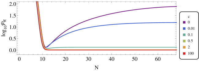
Figure 2: The curvature power spectrum $\mathcal{P}_{\mathcal{R}}$ for the trajectories shown in Fig. 1 corresponding to different colour-coded values of $c$. The curves are normalized relative to the single-field expression, and correspond to the mode that leaves the horizon at the start of the last 60 e-folds of inflation.

As a consequence of the enhancement in $\mathcal{P}_{\mathcal{R}}$, the scalar tilt $n_{s}$ and the tensor-to-scalar ratio $r$ are reduced relative to their values in the single-field chaotic scenario with a quadratic potential, as seen in Fig. 3. In particular, compatibility with the range of $n_{s}$ allowed by Planck is lost for $c\lesssim 0.05$, as seen in the upper panel of Fig. 3. The lower panel of Fig. 3 shows that $r$ has a plateau with a value similar to that in the chaotic quadratic single-field model when the stabilizing parameter $c\lower 3.01385pt\hbox{$\;\stackrel{{\scriptstyle\textstyle>}}{{\sim}}\;$}0.2$, falling to much smaller values as $c\to 0$. Therefore, two-field effects provide a mechanism for suppressing $r$ in this type of quadratic inflationary model, that is complementary to varying the angle of the “bobsleigh track” as discussed in [26].

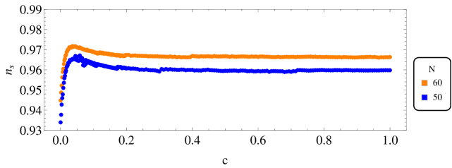
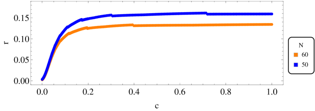
Figure 3: The dependences on the parameter $c$ of the scalar spectral index $n_{s}$ (upper panel) and the tensor-to-scalar ratio $r$ (lower panel), assuming either $N=50$ or $60$ e-folds (blue and orange lines, respectively) and ${\cal R}e~{}T=0$ initially, i.e., $\theta=0$.

The enhancement of the curvature power spectrum is completely negligible for $c\lower 3.01385pt\hbox{$\;\stackrel{{\scriptstyle\textstyle>}}{{\sim}}\;$}1$, where the single-field expressions can be trusted. Therefore, pure quadratic inflation is recovered in the limit of large $c$. Fig. 4 shows the parametric curve $(n_{s}(c),r(c))$ for $c$ decreasing from $1\to 0$ from top to bottom of the plot. This shows that, even with initial conditions along the imaginary direction in the $T$ plane, one can interpolate between BICEP2- and Planck-friendly values of $r\lower 3.01385pt\hbox{$\;\stackrel{{\scriptstyle\textstyle>}}{{\sim}}\;$}0.1,\lower 3.01385pt\hbox{$\;\stackrel{{\scriptstyle\textstyle<}}{{\sim}}\;$}0.1$, respectively, by varying the stabilization parameter $c$. We recall that the modification of the Kähler potential in (57) has no deep theoretical justification. A priori, one might have expected any such modifications of the simple no-scale form (1) to have coefficients that are ${\cal O}(1)$ in natural units, so it is interesting that the naive single-field results would be recovered in this case. This result could perhaps have been expected, since the energy scale during inflation is very small in natural units. We recall that in [26] our default choice was $c=1000$, for which the single-field approximation used there is amply justified. Finally, we note an important feature of Fig. 4 in the limit of small $c$: although $r$ may become as small as in the Starobinsky model, this is possible only for unacceptably small values of $n_{s}$ when an initial condition with ${\cal R}e~{}T=0$, i.e., $\theta=0$, is chosen.

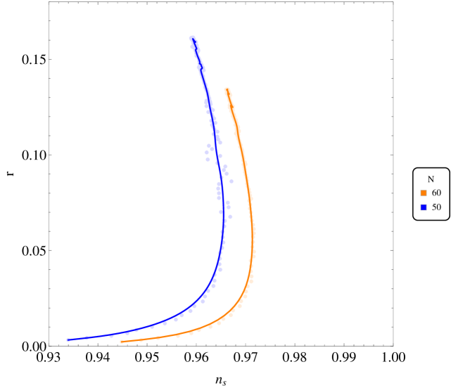
Figure 4: Parametric curve $(n_{s}(c),r(c))$, $c\in(0,1)$ assuming initial conditions with ${\cal R}e~{}T=0$, i.e., $\theta=0$, assuming either $N=50$ or $60$ e-folds (blue and orange lines, respectively).

3.2 ‘Real’ Inflation

We now consider inflation along the direction where ${\cal I}m~{}T=0$, i.e., $\alpha=0$ and $\theta=\pi/2$, with the inflaton identified as ${\cal R}e~{}T$, i.e., $\rho$. We recall that when $\theta=\pi/2$ the imaginary direction is quartically constrained. For this reason, there is no renormalization of any kinetic or mass term as occurred for ‘imaginary’ inflation. In the case of ‘real’ inflation, as we see in Fig. 5, the values of $n_{s}$ and $r$ are essentially identical for any $c\neq 0$. As could be expected, in this direction the no-scale supergravity model has the same predictions as the Starobinsky model, which are completely compatible with the Planck data.

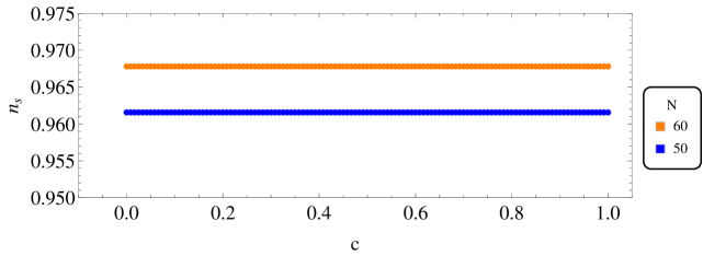
Figure 5: The dependences on the parameter $c$ of the scalar spectral index $n_{s}$ (upper panel) and the tensor-to-scalar ratio $r$ (lower panel), assuming either $N=50$ or $60$ e-folds (blue and orange lines, respectively) assuming ${\cal I}m~{}T=0$ initially, i.e., $\theta=\pi/2$.

3.3 ‘Complex’ Inflation

We showed previously [26] that single-field models interpolating between BICEP2- friendly chaotic quadratic inflation and the Planck-friendly Starobinsky model could be obtained by varying $\theta$ in (57), keeping the stabilization coefficient $c$ large, and we showed in Section 3.1 that two-field effects could also interpolate between the quadratic and Starobinsky predictions even when $\theta=0$. We now explore the possibilities for $0<\theta<\pi/2$ and varying $c$, finding that BICEP2- and/or Planck-compatible predictions for general $\theta>0$ even when the stabilization coefficient $c<1$.

Fig. 6 shows a selection of inflationary trajectories in the $(\rho,\alpha)$ plane for $c=100$ (left panel) and $c=0.1$ (right panel). All the trajectories start from the $N_{\rm tot}=70$ contour line, where $N$ denotes the number of e-folds. In the $c=100$ case, the trajectories are generally convex until they start ‘circling the drain’, with the exception of $\theta=\pi/2$, for which the evolution is strictly along the real axis. However, one sees deviations in the evolution even for angles very close to the real axis. For example, we show in Fig. 6 the trajectory for $\theta=\pi/2(1-\cos(\pi/600))$, which exhibits a substantial departure from the axis at $\rho\approx 1.4$. In the $c=0.1$ case, the trajectories all become concave for small $\rho$ and $\alpha$, and ‘circle the drain’ clockwise.

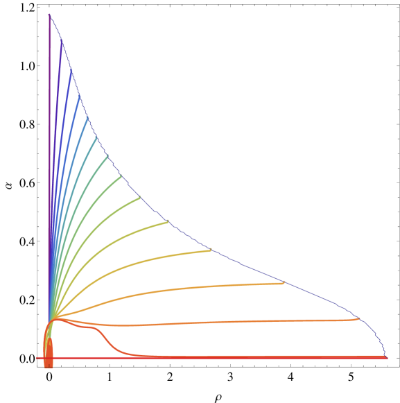
Figure 6: Inflationary trajectories for the Kähler potential (57) at $c=100$ (left panel) and $c=0.1$ (right panel). In both cases, the initial conditions are chosen so as to yield 70 e-folds of inflation. The pure Starobinsky limit is recovered along the real direction ${\cal I}m~{}T(\alpha)=0$.

The enhancement of the power spectrum, $\mathcal{P}_{\mathcal{R}}$, is shown as a function of $\theta$ in Fig. 7 for $c=100$ (upper panel) and $c=0.1$ (lower panel). In the $c=100$ case, the enhancement is generally $\lesssim 2$%, apart from a small enhancement to nearly 4% for $\theta\sim\pi/2$, which is associated with the irregular behaviour of the corresponding trajectory in the left panel of Fig. 6. As could be anticipated from the right panel in Fig. 6, the behaviour of $\mathcal{P}_{\mathcal{R}}$ for $c=0.1$ is more regular, first rising from $\sim 1.4$ to $\sim 1.8$ and then decreasing towards negligible values as $\theta\to 0$.

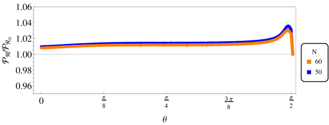
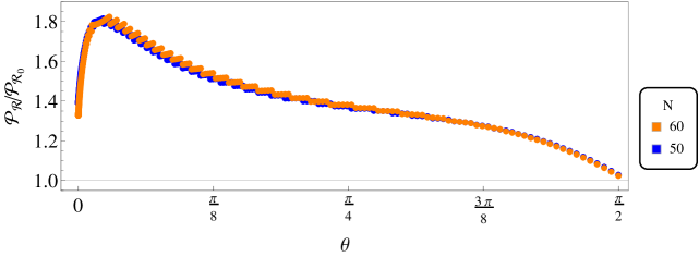
Figure 7: The curvature power spectrum normalized to the single-field expression, $\mathcal{P}_{\mathcal{R}}$, for the mode that leaves the horizon at the start of the last $N=50$ (blue) or $60$ (orange) e-folds of inflation is shown as a function of $\theta$ for $c=100$ (upper panel) and for $c=0.1$ (lower panel).

The bottom part of Fig. 7 corresponds to weak stabilization, $c=0.1$. In this case, the kinetic coupling between the real and imaginary parts of $T$ is still sufficiently strong to cause the inflationary trajectory to deviate from the expected path along the valley of the inflationary potential, for small $\theta$. This is visible in the violet and blue trajectories in Fig. 6, which bend towards the real direction. As a result, a peak in the power spectrum develops at $\theta\gtrsim 0$. At $\theta=0$ the stabilization is purely quadratic (see Eq. (57)) and the power spectrum shows a milder enhancement.

In contrast, the power spectrum at $c=100$ shows a peak at $\theta\simeq\pi/2$, which is a result of the weaker quartic stabilization that dominates near $\theta=\pi/2$. The scalar potential is very flat for $\rho\lesssim 3$, and the kinetic coupling drives the imaginary part $\alpha$ to values away from the minimum of the inflationary valley, As a result, two-field effects are important (see the red trajectory near $\theta=\pi/2$ in Fig. 6), and the power spectrum is enhanced. The large value of $c$ confines the motion of the fields to a narrow valley, and the enhancement is therefore not as dramatic as it is for small $c$. However, at $\theta=\pi/2$ the kinetic coupling vanishes, and inflation is purely single-field.

For intermediate $c$, the power spectrum generally exhibits some combination of both features, which become of comparable size for $c\simeq 0.3$. For $c<0.3$ the largest enhancement is due to the weakness of the stabilization parameter, whereas for $c>0.3$ the peak is due to the weaker quartic stabilization near the real axis. For $c=0.3$, the power spectrum is enhanced by a factor between 1.1 and 1.2 over a broad range in $\theta$ between $\pi/40$ and $7\pi/16$.

The corresponding values of $n_{s}$ at $N=50$ (blue) and 60 (orange) e-folds are shown in Fig. 8 for $c=100$ (upper panel) and $c=0.1$ (lower panel). When $c=100$, we find that $0.95\lesssim n_{s}\lesssim 0.97$ for both the displayed values of $N$ at all values of $\theta$. The only notable feature is a downward glitch at $\theta\sim\pi/2$, which is associated with the corresponding excursion in the inflaton trajectory seen in the left panel of Fig. 6. In contrast, when $c=0.1$ $n_{s}$ initially decreases for small $\theta$ and then increases monotonically as $\theta\to\pi/2$, with values in the acceptable range $0.95\lesssim n_{s}\lesssim 0.97$ for both $N=50$ and $N=60$.

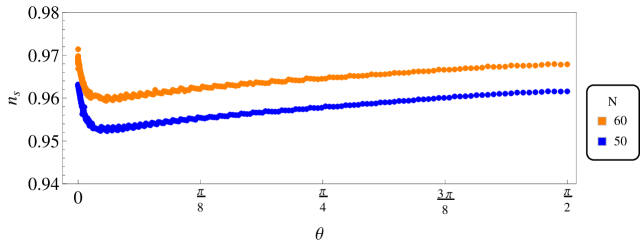
Figure 8: Dependences of the spectral index $n_{s}$ on the angle $\theta$ at $N=50$ (blue lines) and $60$ e-folds (orange lines) for $c=100$ (upper panel) and $c=0.1$ (lower panel).

The corresponding values of $r$ at $N=50$ (blue) and 60 (orange) e-folds are shown in Fig. 9 for $c=100$ (upper panel) and $c=0.1$ (lower panel). In the large-$c$ case, we see a smooth interpolation between BICEP2- and Planck-friendly values of $r$ as $\theta$ increases from $0\to\pi/2$. In the small-$c$ case, the value of $r$ is small except for very small $\theta$, and is in fact below 0.03 for most values of $\theta$.

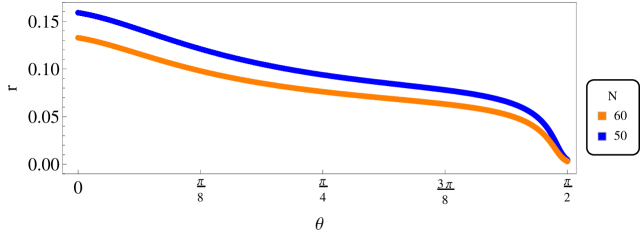
Figure 9: Dependences of the tensor-to-scalar ratio $r$ on the angle $\theta$ at $N=50$ (blue lines) and $60$ e-folds (orange lines) for $c=100$ (upper panel) and $c=0.1$ (lower panel).

The correlations in the behaviours of $n_{s}$ and $r$ are seen in Fig. 10, which displays the parametric curves $(n_{s}(\theta),r(\theta))$ for $N=50$ (blue lines) and $60$ e-folds (orange lines) for $c=100$ (left panel) and $c=0.1$ (right panel). It is clear from the left panel that an interpolation between BICEP2- and Planck-friendly values of $(n_{s},r)$ is possible with $c\gg 1$ as argued in [26], even when two-field effects are taken into account. On the other hand, as seen in the right panel, when $c=0.1$ only small, Planck-friendly values of $r$ are found.

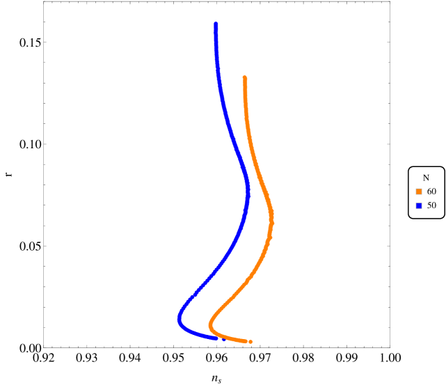
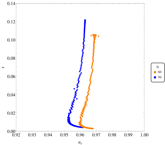
Figure 10: Parametric curve $(n_{s}(\theta),r(\theta))$ for $c=100$ (left panel) and $c=0.1$ (right panel), both for $N=50$ (blue) and $60$ (orange) e-folds.

All the above results are for a total number $N_{\rm tot}=70$ of e-folds, and we now explore the possible modifications of the above results for larger values of $N_{\rm tot}$. Fig. 11 shows the total number of e-folds $N_{\rm tot}$ as a function of the initial conditions in the $(\rho,\alpha)$ plane for $c=100$ (left panel) and $c=0.1$ (right panel), with solid lines corresponding to $N=50$ (lower) and $N=60$ (upper). Each point in the plane corresponds to the particular form of the Kähler potential (and therefore of the scalar potential) for which the stabilizing term vanishes initially,

$$\tan\theta=\frac{3}{2\alpha_{0}^{2}}\left(e^{-\sqrt{\frac{2}{3}}\rho_{0}}-1\right),$$ (61)

i.e., the initial condition is chosen at the bottom of the inflationary valley. We see that when $c=0.1$ the variation of $N_{\rm tot}$ in the displayed part of the $(\rho,\alpha)$ plane is much greater than for $c=100$, and much larger values of $N_{\rm tot}$ may be attained, though one should bear in mind that the canonical field along the imaginary axis is related to $\alpha$ in a $c$-dependent way as shown in Eq. (59).

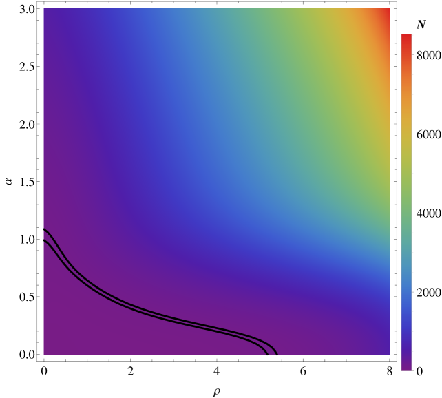
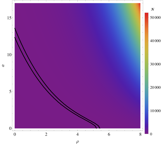
Figure 11: The total number of e-folds $N_{\rm tot}$ as a function of the fields in the $(\rho,\alpha)$ plane, for $c=100$ (left panel) and $c=0.1$ (right panel). The solid black lines correspond to $N=50$ (lower) and $N=60$ (upper).

Fig. 12 displays general results for $n_{s}$ in the $(\rho,\alpha)$ plane. The upper (lower) panels are for $c=100$ ($c=0.1$), and the left (right) panels are for $N=50(60)$ e-folds. In the case $N=50$ and $c=100$, we see that there is a large region of the $(\rho,\alpha)$ plane with $\alpha\gtrsim 1.5$ where $n_{s}\simeq 0.960$. Larger values or $n_{s}\lesssim 0.970$ are found in a band around $\alpha\sim 1.0$, and smaller values $n_{s}\gtrsim 0.950$ are found for $\alpha<0.5$. Acceptable values of $n_{s}$ are found throughout the $(\rho,\alpha)$ plane for $N=50,c=100$. The general behaviour in the $N=60,c=100$ case is very similar, but the values of $n_{s}$ are larger by $\sim 0.008$ corresponding approximately to one current standard deviation, and there is a band with $\alpha\sim 1.0$ where $n_{s}\gtrsim 0.970$. In the case $N=50,c=0.1$, there is relatively little variation in $n_{s}$, with values generally $\simeq 0.960$. There is also relatively little variation in $n_{s}$ across the $(\rho,\alpha)$ plane for $N=60,c=0.1$, but the values are again generally larger by $\sim 0.008$.

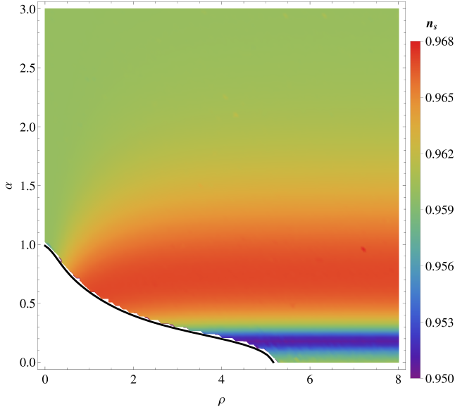
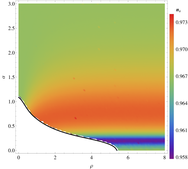
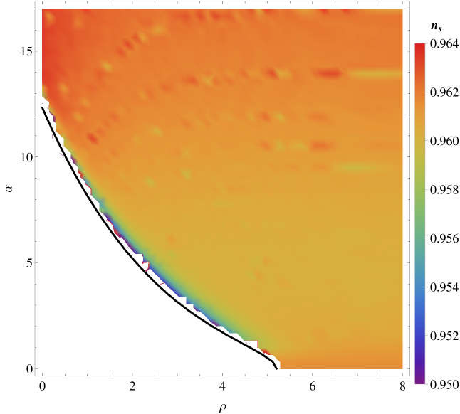
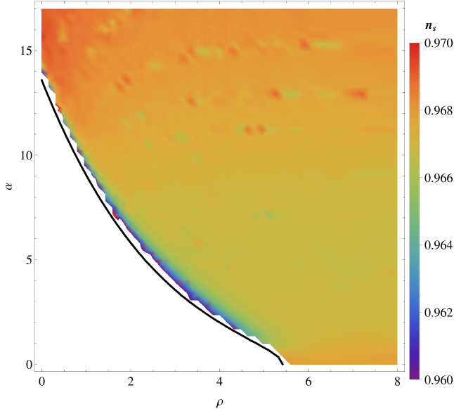
Figure 12: Scalar spectral index $n_{s}$ from the two-field analysis in the $(\rho,\alpha)$ plane, evaluated at $N=50$ (left panels) and $60$ (right panels) e-folds, with $c=100$ (upper panels) and $c=0.1$ (lower panels). The solid curves are the boundaries for the corresponding values of $N$.

Fig. 13 shows corresponding results for $r$ in the $(\rho,\alpha)$ plane. In the $c=100$ cases (upper panels), we see that BICEP2-friendly values of $r\gtrsim 0.10$ are found for $\alpha\gtrsim 1.7$ for all values of $\rho$, extending down to $\alpha\sim 1$ for $\rho\lesssim 1$. We also see that $r\lesssim 0.03$ for $\alpha<0.3$. In the case $N=50,c=0.1$, we see that values of $r$ interpolate smoothly between the BICEP2-friendly values found at small $\theta$ and the Planck-friendly values found when $\theta\sim\pi/2$. The values of $r$ for $N=60,c=0.1$ are slightly lower, but also interpolate smoothly between BICEP2- and Planck-friendly values.

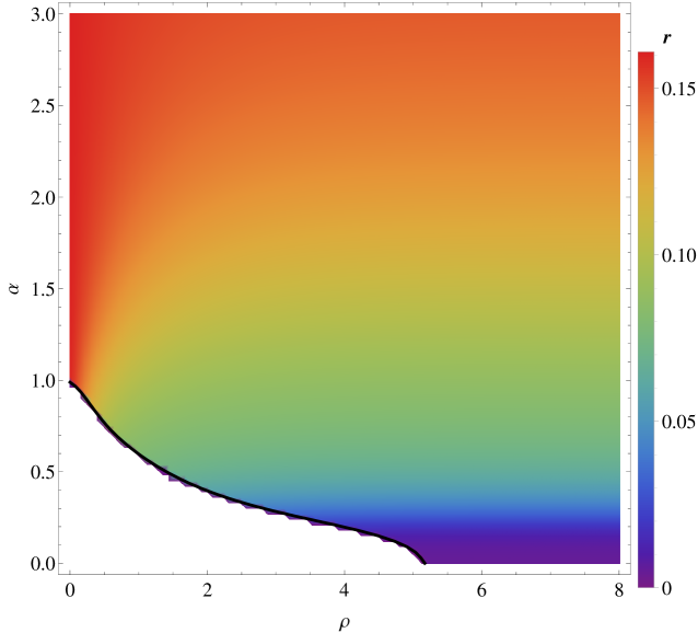
Figure 13: Tensor-to-scalar ratio $r$ from the two-field analysis in the $(\rho,\alpha)$ plane, evaluated at $N=50$ (left panels) and $60$ (right panels) e-folds, with $c=100$ (upper panels) and $c=0.1$ (lower panels). The solid curves are the boundaries for the corresponding values of $N$.

4 Non-Gaussianity

The two-field formalism used above relies on the assumption that the scalar field fluctuations are nearly Gaussian, an assumption that clearly needs to be verified. A quantitative measure of non-Gaussianity is provided by the dimensionless nonlinear parameter $f_{\rm NL}$, which is related to the bispectrum by [60]

$$\mathcal{B}_{\mathcal{R}}(k_{1},k_{2},k_{3})\;\equiv\;-\frac{6}{5}f_{\rm NL}(k_{1},k_{2},k_{3})[\mathcal{P}_{\mathcal{R}}(k_{1})\mathcal{P}_{\mathcal{R}}(k_{2})+{\rm cyclic}]\,.$$ (62)

For bispectrum configurations of the local type (e.g., $k_{1}\simeq k_{2}\gg k_{3}$), $f_{\rm NL}$ can be calculated using the $\delta N$ formalism [61, 62, 63]. Namely, for Lagrangian of the form

$$\mathcal{L}\;=\;\frac{1}{2}G_{ij}\partial_{\mu}\phi^{i}\partial^{\mu}\phi^{j}-V(\phi^{1},\phi^{2})$$ (63)

with the gradients with respect to the fields defined as

$$\nabla\;\equiv\;(\partial_{i})\ ,\ \ \nabla^{T}\equiv(G^{ij}\partial_{j})\,,$$ (64)

one finds that

$$f_{\rm NL}\;=\;-\frac{5}{6}\frac{\nabla N\nabla^{T}\nabla N\nabla^{T}N}{|\nabla N|^{4}}\,,$$ (65)

where $N$ is the number of e-foldings, and the gradients are evaluated at horizon exit. In our particular case, in the non-canonical basis

$$T=\frac{1}{\sqrt{2}}(x+iy)$$ (66)

the expression (65) conveniently reduces to

$$f_{\rm NL}=-\frac{5}{6}\frac{N_{ij}N_{i}N_{j}}{(N_{i}^{2})^{2}}\,.$$ (67)

Some results for $f_{\rm NL}$ in the $(\rho,\alpha)$ planes for $c=100$ and $c=0.1$ are displayed in Fig. 14 .

The upper panels in Fig. 14 show the values of $f_{\rm NL}$ in the $(\rho,\alpha)$ plane for $c=100$, and the lower panels show results for $c=0.1$. The left (right) panels assume a horizon exit 50 (60) e-folds before the end of inflation. Since, as we saw previously, two-field effects are generally small for $c=100$, with no significant enhancement of the scalar power spectrum and values of $n_{s}$ and $r$ that are generally close to those in the single-field limit, we do not expect large values of $f_{\rm NL}$ in the upper panels. Indeed, we do find values of $f_{\rm NL}$ that are very small, typically $\lesssim 0.015$ in most of the $(\rho,\alpha)$ plane, and attaining values only as large as 0.036 in the limit $\theta\to\pi/2$ corresponding to initial conditions with $\alpha\simeq 0$. This implies that two-field effects are stronger in this limit. This coincides with the behaviour of the power spectrum shown in Fig. (7) and the shape of the inflationary trajectory near $\theta=\pi/2$ shown in Fig. (6). Interestingly, as seen in the lower panel of Fig. 14, we also find small values of $f_{\rm NL}\lesssim 0.032$ even in the case $c=0.1$ where we might have expected two-field effects to be much more important. We conclude that, for all points in the $(\rho,\alpha)$ plane in the cases studied, the assumption of near-Gaussianity is acceptable.

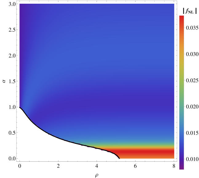
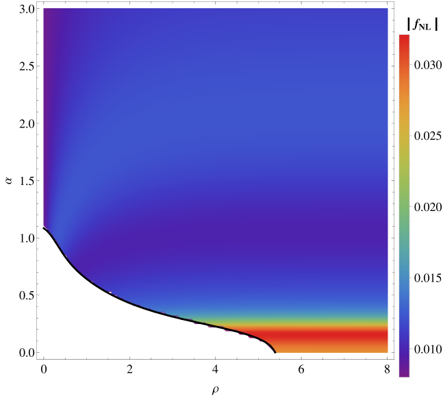
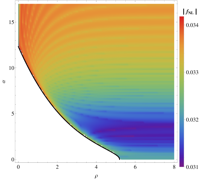
Figure 14: Values of the non-Gaussianity parameter $f_{\rm NL}$ in the $(\rho,\alpha)$ plane, evaluated for $N=50$ (left) and $60$ (right) e-folds, for $c=100$ (upper panel) and $c=0.1$ (lower panel).

5 Summary and Conclusions

We have presented in this paper a general formalism for the study of two-field effects in supergravity models. We have specialized to a particular example in the context of no-scale supergravity motivated by Planck and BICEP2 data. It is known that such models require terms in the Kähler potential that stabilize some field components, and we have studied how sensitive the predictions for the CMB observables $n_{s},r$ are to their magnitude. We have also studied the magnitude of the non-Gaussianity parameter $f_{\rm NL}$ in the presence of two-field effects. Our studies have been within the framework of one particular form for the stabilization terms, but we expect them to have broader validity.

We have found that varying the magnitude of the stabilization terms yields predictions for the tensor-to-scalar ratio $r$ that interpolate between large BICEP2-friendly values $\sim 0.15$ to much smaller Planck-friendly values. This is possible along a fixed direction in field space, whereas in the single-field approximation (which applies when the stabilization is strong) such a BICEP2-Planck interpolation is possible only by varying the inflationary direction in field space [26]. The new degree of flexibility in the two-field case is due to the enhancement $\mathcal{P}_{\mathcal{R}}$ of the scalar power spectrum in the two-field case. This mechanism may offer a way of resuscitating quadratic chaotic inflationary models, which would otherwise yield large values of $r$ that seem to be disfavoured [7] by the recent Planck data on dust in the BICEP2 field of view [6], if they are embedded in a broader framework.

In general, our two-field analysis yields values of the scalar spectral tilt $n_{s}$ that are highly compatible with the range currently favoured by experiment. It was known previously that the no-scale supergravity model yields acceptable values of $n_{s}$ when treated in the single-field approximation appropriate for large stabilization terms. It is reassuring that this concordance is not lost when their magnitude is reduced.

It is also reassuring that our two-field analysis yields value of $f_{\rm NL}$ that are within the experimental upper bounds. Indeed, our small results for $f_{\rm NL}$ give little encouragement that this type of non-Gaussianity could be measured within the foreseeable future.

Finally, we note that the analysis made here can easily be extended to other supergravity models of inflation. As mentioned earlier, a multi-field treatment is likely to be required for such models, since they are generally described by effective theories with more than one field. Our results suggest that, on the one hand, such models are likely capable of yielding results compatible with current CMB observations at least as long as any stabilization terms have characteristic energy scales larger than the inflation scale. On the other hand, our results show how models that appear to yield large values of $r$ in the single-field approximation can yield much smaller values of $r$ when two-field effects become important. This feature may become welcome if dust effects are as significant for the interpretation of the BICEP2 data as has been suggested in [4, 6]. We look forward to the promised upcoming joint publication by the BICEP2 and Planck collaborations, and to data from other experiments.

References

- [1] P. A. R. Ade et al. [Planck Collaboration], arXiv:1303.5082 [astro-ph.CO].
- [2] P. A. R. Ade et al. [BICEP2 Collaboration], Phys. Rev. Lett. 112, 241101 (2014) [arXiv:1403.3985 [astro-ph.CO]].
- [3] G. Hinshaw et al. [WMAP Collaboration], Astrophys. J. Suppl. 208 (2013) 19 [arXiv:1212.5226 [astro-ph.CO]]; for a recent review, see E. Komatsu et al. [on behalf of the WMAP Science Team Collaboration], arXiv:1404.5415 [astro-ph.CO].
- [4] H. Liu, P. Mertsch and S. Sarkar, Astrophys. J. 789, L29 (2014) [arXiv:1404.1899 [astro-ph.CO]]; M. J. Mortonson and U. Seljak, arXiv:1405.5857 [astro-ph.CO]; R. Flauger, J. C. Hill and D. N. Spergel, JCAP 1408, 039 (2014) [arXiv:1405.7351 [astro-ph.CO]]; M. Cort s, A. R. Liddle and D. Parkinson, arXiv:1409.6530 [astro-ph.CO].
- [5] C. R. Contaldi, M. Peloso and L. Sorbo, JCAP 1407, 014 (2014) [arXiv:1403.4596 [astro-ph.CO]]; V. Miranda, W. Hu and P. Adshead, arXiv:1403.5231 [astro-ph.CO]; K. M. Smith, C. Dvorkin, L. Boyle, N. Turok, M. Halpern, G. Hinshaw and B. Gold, Phys. Rev. Lett. 113, 031301 (2014) [arXiv:1404.0373 [astro-ph.CO]].
- [6] R. Adam et al. [ Planck Collaboration], arXiv:1409.5738 [astro-ph.CO].
- [7] C. Cheng, Q. G. Huang and S. Wang, arXiv:1409.7025 [astro-ph.CO].
- [8] A. A. Starobinsky, Phys. Lett. B 91, 99 (1980).
- [9] V. F. Mukhanov and G. V. Chibisov, JETP Lett. 33, 532 (1981) [Pisma Zh. Eksp. Teor. Fiz. 33, 549 (1981)].
- [10] A. A. Starobinsky, Sov. Astron. Lett. 9, 302 (1983).
- [11] F. Bezrukov and M. Shaposhnikov, JHEP 0907, 089 (2009) [arXiv:0904.1537 [hep-ph]].
- [12] J. Ellis, D. V. Nanopoulos and K. A. Olive, Phys. Rev. Lett. 111 (2013) 111301 [arXiv:1305.1247 [hep-th]];
- [13] J. Ellis, D. V. Nanopoulos and K. A. Olive, JCAP 1310 (2013) 009 [arXiv:1307.3537 [hep-th]];
- [14] R. Kallosh and A. Linde, JCAP 1306, 028 (2013) [arXiv:1306.3214 [hep-th]].
- [15] W. Buchmuller, V. Domcke and K. Kamada, Phys. Lett. B 726, 467 (2013) [arXiv:1306.3471 [hep-th]].
- [16] F. Farakos, A. Kehagias and A. Riotto, Nucl. Phys. B 876, 187 (2013) [arXiv:1307.1137].
- [17] J. Ellis, D. V. Nanopoulos and K. A. Olive, Phys. Rev. D 89, 043502 (2014) [arXiv:1310.4770 [hep-ph]].
- [18] S. Ferrara, R. Kallosh, A. Linde and M. Porrati, Phys. Rev. D 88, no. 8, 085038 (2013) [arXiv:1307.7696 [hep-th]]; S. Ferrara, R. Kallosh, A. Linde and M. Porrati, JCAP 1311, 046 (2013) [arXiv:1309.1085 [hep-th], arXiv:1309.1085]; S. Ferrara, R. Kallosh and A. Van Proeyen, JHEP 1311, 134 (2013) [arXiv:1309.4052 [hep-th]]; S. Cecotti and R. Kallosh, JHEP 1405, 114 (2014) [arXiv:1403.2932 [hep-th]].
- [19] J. Alexandre, N. Houston and N. E. Mavromatos, Phys. Rev. D 89 (2014) 027703 [arXiv:1312.5197 [gr-qc]]; J. Ellis, N. E. Mavromatos and D. V. Nanopoulos, Phys. Lett. B 732, 380 (2014) [arXiv:1402.5075 [hep-th]].
- [20] C. Pallis, JCAP 1404, 024 (2014) [arXiv:1312.3623 [hep-ph]].
- [21] I. Antoniadis, E. Dudas, S. Ferrara and A. Sagnotti, Phys. Lett. B 733, 32 (2014) [arXiv:1403.3269 [hep-th]].
- [22] K. Kamada and J. Yokoyama, arXiv:1405.6732 [hep-th].
- [23] C. Kounnas, D. L st and N. Toumbas, arXiv:1409.7076 [hep-th].
- [24] J. Ellis, N. E. Mavromatos and D. J. Mulryne, JCAP 1405, 012 (2014) [arXiv:1401.6078 [astro-ph.CO]].
- [25] K. Turzyńsky, [arXiv:1405.6195 [astro-ph.CO]];
- [26] J. Ellis, M. A. G. Garcia, D. V. Nanopoulos and K. A. Olive, JCAP 1408, 044 (2014) [arXiv:1405.0271 [hep-ph]].
- [27] S. Tsujikawa, D. Parkinson and B. A. Bassett, Phys. Rev. D 67, 083516 (2003) [astro-ph/0210322].
- [28] Z. Lalak, D. Langlois, S. Pokorski and K. Turzynski, JCAP 0707, 014 (2007) [arXiv:0704.0212 [hep-th]].
- [29] C. van de Bruck and M. Robinson, arXiv:1404.7806 [astro-ph.CO].
- [30] J. R. Ellis, D. V. Nanopoulos, K. A. Olive and K. Tamvakis, Phys. Lett. B 118 (1982) 335; Phys. Lett. B 120 (1983) 331; Nucl. Phys. B 221 (1983) 52.
- [31] D. V. Nanopoulos, K. A. Olive, M. Srednicki and K. Tamvakis, Phys. Lett. B 123, 41 (1983).
- [32] R. Holman, P. Ramond and G. G. Ross, Phys. Lett. B 137, 343 (1984).
- [33] A. B. Goncharov and A. D. Linde, Phys. Lett. B 139, 27 (1984).
- [34] D. Z. Freedman, P. van Nieuwenhuizen and S. Ferrara, Phys. Rev. D 13 (1976) 3214; S. Deser and B. Zumino, Phys. Lett. B 62 (1976) 335.
- [35] A. D. Linde, Nucl. Phys. B 252, 153 (1985); M. S. Madsen and P. Coles, Nucl. Phys. B 298, 701 (1988).
- [36] E. J. Copeland, A. R. Liddle, D. H. Lyth, E. D. Stewart and D. Wands, Phys. Rev. D 49, 6410 (1994) [astro-ph/9401011]; E. D. Stewart, Phys. Rev. D 51, 6847 (1995) [hep-ph/9405389].
- [37] M. Kawasaki, M. Yamaguchi and T. Yanagida, Phys. Rev. Lett. 85, 3572 (2000) [arXiv:hep-ph/0004243].
- [38] M. Yamaguchi and J. Yokoyama, Phys. Rev. D 63, 043506 (2001) [arXiv:hep-ph/0007021]; M. Yamaguchi, Phys. Rev. D 64, 063502 (2001) [arXiv:hep-ph/0103045]; M. Kawasaki and M. Yamaguchi, Phys. Rev. D 65, 103518 (2002) [arXiv:hep-ph/0112093]; M. Yamaguchi and J. Yokoyama, Phys. Rev. D 68 (2003) 123520 [arXiv:hep-ph/0307373]; P. Brax and J. Martin, Phys. Rev. D 72, 023518 (2005) [arXiv:hep-th/0504168]; K. Kadota and M. Yamaguchi, Phys. Rev. D 76, 103522 (2007) [arXiv:0706.2676 [hep-ph]]; F. Takahashi, Phys. Lett. B 693, 140 (2010) [arXiv:1006.2801 [hep-ph]]; K. Nakayama and F. Takahashi, JCAP 1011, 009 (2010) [arXiv:1008.2956 [hep-ph]]; K. Nakayama, F. Takahashi and T. T. Yanagida, Phys. Lett. B 725, 111 (2013) [arXiv:1303.7315 [hep-ph]]; K. Nakayama, F. Takahashi and T. T. Yanagida, JCAP 1308, 038 (2013) [arXiv:1305.5099, arXiv:1305.5099 [hep-ph]]; K. Harigaya, M. Ibe, K. Schmitz and T. T. Yanagida, Phys. Lett. B 733, 283 (2014) [arXiv:1403.4536 [hep-ph]]; K. Harigaya and T. T. Yanagida, arXiv:1403.4729 [hep-ph]; K. Harigaya, M. Ibe, K. Ichikawa, K. Kaneta and S. Matsumoto, arXiv:1403.5880 [hep-ph]. K. Harigaya and T. T. Yanagida, arXiv:1407.1580 [hep-ph]; K. Nakayama, F. Takahashi and T. T. Yanagida, Phys. Lett. B 737, 151 (2014) [arXiv:1407.7082 [hep-ph]].
- [39] H. Murayama, H. Suzuki, T. Yanagida and J.-i. Yokoyama, Phys. Rev. Lett. 70 (1993) 1912 and Phys. Rev. D 50 (1994) 2356 [hep-ph/9311326]; J. R. Ellis, M. Raidal and T. Yanagida, Phys. Lett. B 581 (2004) 9 [hep-ph/0303242]; K. Nakayama, F. Takahashi and T. T. Yanagida, Phys. Lett. B 730, 24 (2014) [arXiv:1311.4253 [hep-ph]].
- [40] S. C. Davis and M. Postma, JCAP 0803, 015 (2008) [arXiv:0801.4696 [hep-ph]]; R. Kallosh and A. Linde, JCAP 1011, 011 (2010) [arXiv:1008.3375 [hep-th]]; R. Kallosh, A. Linde and T. Rube, Phys. Rev. D 83, 043507 (2011) [arXiv:1011.5945 [hep-th]]; R. Kallosh, A. Linde, K. A. Olive and T. Rube, Phys. Rev. D 84, 083519 (2011) [arXiv:1106.6025 [hep-th]]; M. A. G. Garcia and K. A. Olive, JCAP 1309, 007 (2013) [arXiv:1306.6119 [hep-ph]]; T. Li, Z. Li and D. V. Nanopoulos, arXiv:1405.0197 [hep-th]; W. Buchmuller, C. Wieck and M. W. Winkler, arXiv:1404.2275 [hep-th]; W. Buchmuller, E. Dudas, L. Heurtier and C. Wieck, arXiv:1407.0253 [hep-th].
- [41] E. Cremmer, S. Ferrara, C. Kounnas and D. V. Nanopoulos, Phys. Lett. B 133 (1983) 61; J. R. Ellis, A. B. Lahanas, D. V. Nanopoulos and K. Tamvakis, Phys. Lett. B 134 (1984) 429; A. B. Lahanas and D. V. Nanopoulos, Phys. Rept. 145 (1987) 1.
- [42] E. Witten, Phys. Lett. B 155, 151 (1985).
- [43] A. S. Goncharov and A. D. Linde, Class. Quant. Grav. 1, L75 (1984); H. Murayama, H. Suzuki, T. Yanagida and J. Yokoyama, Phys. Rev. D 50, 2356 (1994) [arXiv:hep-ph/9311326].
- [44] J. R. Ellis, K. Enqvist, D. V. Nanopoulos, K. A. Olive and M. Srednicki, Phys. Lett. B 152 (1985) 175 [Erratum-ibid. 156B (1985) 452]; K. Enqvist, D. V. Nanopoulos and M. Quiros, Phys. Lett. B 159, 249 (1985); T. Li, Z. Li and D. V. Nanopoulos, arXiv:1310.3331 [hep-ph].
- [45] P. Binétruy and M. K. Gaillard, Phys. Rev. D 34, 3069 (1986).
- [46] S. Antusch, M. Bastero-Gil, K. Dutta, S. F. King and P. M. Kostka, JCAP 0901, 040 (2009) [arXiv:0808.2425 [hep-ph]]; S. Antusch, M. Bastero-Gil, K. Dutta, S. F. King and P. M. Kostka, Phys. Lett. B 679, 428 (2009) [arXiv:0905.0905 [hep-th]].
- [47] J. Ellis, M. A. G. Garc a, D. V. Nanopoulos and K. A. Olive, JCAP 1405, 037 (2014) [arXiv:1403.7518 [hep-ph]].
- [48] R. Kallosh and A. Linde, JCAP 1307, 002 (2013) [arXiv:1306.5220 [hep-th]]; R. Kallosh and A. Linde, JCAP 1310, 033 (2013) [arXiv:1307.7938]; R. Kallosh and A. Linde, JCAP 1312, 006 (2013) [arXiv:1309.2015 [hep-th]]; R. Kallosh, A. Linde and D. Roest, Phys. Rev. Lett. 112, no. 1, 011303 (2014) [arXiv:1310.3950 [hep-th]]; R. Kallosh, A. Linde and D. Roest, JHEP 1311, 198 (2013) [arXiv:1311.0472 [hep-th]]; R. Kallosh, A. Linde and D. Roest, JHEP 1408, 052 (2014) [arXiv:1405.3646 [hep-th]]; R. Kallosh, A. Linde and D. Roest, arXiv:1407.4471 [hep-th].
- [49] S. Cecotti, Phys. Lett. B 190 (1987) 86.
- [50] S. Ferrara, A. Kehagias and A. Riotto, Fortsch. Phys. 62, 573 (2014) [arXiv:1403.5531 [hep-th]]; S. Ferrara, A. Kehagias and A. Riotto, arXiv:1405.2353 [hep-th].
- [51] R. Kallosh, A. Linde, B. Vercnocke and W. Chemissany, JCAP 1407, 053 (2014) [arXiv:1403.7189 [hep-th]]; K. Hamaguchi, T. Moroi and T. Terada, Phys. Lett. B 733, 305 (2014) [arXiv:1403.7521 [hep-ph]].
- [52] J. A. Casas, in Proceedings, International Europhysics Conference on High-Energy Physics, Jerusalem, Israel, August 19-25, 1997, eds. D. Lellouch, G. Mikenberg and E. Rabinovici, pp 914-917 [hep-ph/9802210].
- [53] C. Gordon, D. Wands, B. A. Bassett and R. Maartens, Phys. Rev. D 63, 023506 (2001) [astro-ph/0009131]; C. T. Byrnes and D. Wands, Phys. Rev. D 74, 043529 (2006) [astro-ph/0605679]; R. Easther, J. Frazer, H. V. Peiris and L. C. Price, Phys. Rev. Lett. 112 (2014) 161302 [arXiv:1312.4035 [astro-ph.CO]];
- [54] J. Garcia-Bellido and D. Wands, Phys. Rev. D 52, 6739 (1995) [gr-qc/9506050]; A. A. Starobinsky, S. Tsujikawa and J. Yokoyama, Nucl. Phys. B 610, 383 (2001) [astro-ph/0107555]; F. Di Marco, F. Finelli and R. Brandenberger, Phys. Rev. D 67, 063512 (2003) [astro-ph/0211276]; F. Di Marco and F. Finelli, Phys. Rev. D 71, 123502 (2005) [astro-ph/0505198]; K. Y. Choi, L. M. H. Hall and C. van de Bruck, JCAP 0702, 029 (2007) [astro-ph/0701247];
- [55] V. F. Mukhanov and P. J. Steinhardt, Phys. Lett. B 422, 52 (1998) [astro-ph/9710038].
- [56] D. Langlois and S. Renaux-Petel, JCAP 0804, 017 (2008) [arXiv:0801.1085 [hep-th]]; C. M. Peterson and M. Tegmark, Phys. Rev. D 83, 023522 (2011) [arXiv:1005.4056 [astro-ph.CO]].
- [57] I. Antoniadis, E. Dudas, S. Ferrara and A. Sagnotti, Phys. Lett. B 733, 32 (2014) [arXiv:1403.3269 [hep-th]]; S. Ferrara, R. Kallosh and A. Linde, arXiv:1408.4096 [hep-th]; R. Kallosh and A. Linde, arXiv:1408.5950 [hep-th].
- [58] C. M. Peterson and M. Tegmark, Phys. Rev. D 87, no. 10, 103507 (2013) [arXiv:1111.0927 [astro-ph.CO]].
- [59] J. M. Bardeen, Phys. Rev. D 22, 1882 (1980).; J. M. Stewart, Class. Quant. Grav. 7, 1169 (1990).
- [60] E. Komatsu and D. N. Spergel, Phys. Rev. D 63, 063002 (2001) [astro-ph/0005036].
- [61] D. H. Lyth and Y. Rodriguez, Phys. Rev. Lett. 95, 121302 (2005) [astro-ph/0504045].
- [62] C. M. Peterson and M. Tegmark, Phys. Rev. D 83, 023522 (2011) [arXiv:1005.4056 [astro-ph.CO]].
- [63] C. M. Peterson and M. Tegmark, Phys. Rev. D 84, 023520 (2011) [arXiv:1011.6675 [astro-ph.CO]].