Hydromagnetic Waves in a Compressed Dipole Field via Field-Aligned Klein-Gordon Equations

Abstract

Hydromagnetic waves, especially those of frequencies in the range of a few milli-Hz to a few Hz observed in the Earth’s magnetosphere, are categorized as Ultra Low Frequency (ULF) waves or pulsations. They have been extensively studied due to their importance in the interaction with radiation belt particles and in probing the structures of the magnetosphere. We developed an approach in examining the toroidal standing Aflvén waves in a background magnetic field by recasting the wave equation into a Klein-Gordon (KG) form along individual field lines. The eigenvalue solutions to the system are characteristic of a propagation type when the corresponding eigen-frequency is greater than a cut-off frequency and an evanescent type otherwise. We apply the approach to a compressed dipole magnetic field model of the inner magnetosphere, and obtain the spatial profiles of relevant parameters and the spatial wave forms of harmonic oscillations. We further extend the approach to poloidal mode standing Alfvén waves along field lines. In particular, we present a quantitative comparison with a recent spacecraft observation of a poloidal standing Alfvén wave in the Earth’s magnetosphere. Our analysis based on KG equation yields consistent results which agree with the spacecraft measurements of the wave period and the amplitude ratio between the magnetic field and electric field perturbations. We also present computational results of eigenvalue solutions to the compressional poloidal mode waves in the compressed dipole magnetic field geometry.

1 Introduction

Hydromagnetic waves are common phenomena in space plasmas. The associated magnetic and electric field perturbations are observed both on ground and from space in the Earth’s magnetosphere. Such waves or magnetic pulsations of frequencies less than $\sim 1$ Hz are typically categorized as Ultra Low Frequency (ULF) waves (Fraser, 2006; Kivelson, 2006). They can be further divided into sub-categories, such as Pc1-5, Pi1-3 and Pg, with frequencies ranging from a few Hz down to a few milli-Hz (mHz) (Fraser, 2006; Volwerk, 2006). Generally they exhibit regular and monochromatic magnetic and electric field wave forms. Such waves can be identified as Alfvén waves propagating in the Earth’s magnetosphere, e.g., the recent spacecraft observation by the Van Allen Probe (Radiation Belt Storm Probes) of Dai et al. (2013). Based on the direction or the polarization of the magnetic (or electric) field perturbation in the linearized assumption, they can be further characterized as toroidal and/or poloidal mode waves. In the toroidal mode, the magnetic field perturbation is in the azimuthal direction, i.e., along the east-west longitudinal direction (the accompanying electric field perturbation has a radial component) in Earth’s dipole magnetic field. On the other hand in the poloidal mode, the magnetic field perturbation has a radial component, lying in the meridional plane, while the electric field perturbation is azimuthal.

The basic theory for ULF waves traces back to Tamao (1965) and has been well developed. These waves are interpreted as standing Alfvén (transverse) or fast-mode hydromagnetic waves in cold plasmas immersed in the Earth’s magnetic field (Cummings et al., 1969; Singer et al., 1981; Southwood and Hughes, 1983). Their characteristics are closely governed by the geometry of the background magnetic field and the associated plasma density distribution. More general and sophisticated numerical simulations were also developed in recent years to take into account more realistic background field topology, multiple physical effects, and non-idealized boundary conditions (Kabin et al., 2007; Lee and Takahashi, 2006; Claudepierre et al., 2010). The study of ULF waves has important implications for wave-particle interaction and diagnostics of magnetospheric structures. In particular, it has been established the critical role that ULF waves play in the energization and transport of radiation belt particles based on both theoretical and observational studies (Elkington, 2006; Elkington et al., 2003, 1999; Takahashi et al., 2002; Ukhorskiy et al., 2005).

An alternative approach to describing the toroidal (transverse) Alfvén standing waves in an axi-symmetric background magnetic field has been given by McKenzie and Hu (2010) where the wave equations were cast along an individual field line and transformed into a Klein-Gordon (KG) form. This approach was further formalized and applied to the Earth’s dipole magnetic field. We later showed in great detail the formulation and procedures of the approach for a given background field topology and density distribution in Webb et al. (2012). The eigen-frequencies obtained from the eigen-mode solutions to the KG equations correspond well to the ULF waves frequencies in the Pc3-5 range (Webb et al., 2012). The same approach was also successfully applied to coronal loop oscillations in low corona under different background field and plasma conditions (Hu et al., 2012). In the present work, we first apply the approach to a more realistic Earth’s background field as represented by a compressed dipole model of Kabin et al. (2007). We derive the eigen-frequencies and eigen-functions of the wave forms for this particular geometry corresponding to the toroidal mode and compare with the results from other similar studies.

Furthermore, motivated by a recent direct observation of poloidal standing Alfvén waves in Earth’s magnetosphere by Dai et al. (2013) (see also, Takahashi et al., 2013; Liu et al., 2013, 2011), we extend our investigation to examine the poloidal mode waves as well. In the case of a transverse poloidal mode, the wave equation can also be cast into a KG form along a field line. We numerically solve the wave equation for electric field perturbation. The corresponding magnetic field perturbation can be obained in a similar manner to the approach based on KG equations for the toroidal mode. In Dai et al. (2013), a case of a fundamental mode standing poloidal wave was identified from the newly launched Van Allen Probe (Radiation Belt Storm Probes) spacecraft measurements. They obtained wave period of the azimuthal electric field and the associated radial magnetic field oscillations, the relative ratio of wave amplitudes, and the relative phase shift at the spacecraft location in the inner magnetosphere. Their analysis provided clear evidence for the existence of poloidal mode waves and their interaction with particles.

The article is organized as follows. Section 2 provides a brief summary of the toroidal-mode wave equations and their transformation into the KG form. The general approach of solving the resulting eigenvalue problem is described and applied to a compressed dipole magnetic field model of Earth’s magnetosphere. The eigen-frequencies and the corresponding wave-form solutions are presented. Section 3 extends the analysis to the decoupled eigenvalue solutions of the poloidal mode waves for a given geometry, and presents a comparison with the solution from other approaches and with observations, especially for the transverse Alfvén waves. We finally summarize our results in the last section.

2 Klein-Gordon Equations for the Toroidal Mode

We first consider toroidal wave perturbations ($b_{\phi},u_{\phi}$) in the magnetic field and fluid velocity in a background axi-symmetric (that is azimuthal wave number $m=0$) magnetic field $\vec{B}_{0}=(B_{r},B_{\theta},0)$, in spherical coordinates $(r,\theta,\phi)$. The perturbation electric field $\vec{E}$ is given by

$$\vec{E}=-\vec{u}\times\vec{B}=-u_{\phi}B_{r}\hat{\theta}+u_{\phi}B_{\theta}\hat{r}=E_{n}\hat{n},$$ (1)

normal to the background magnetic field line. The $\phi$ (toroidal) components of Faraday’s law and the momentum equation yield the following wave equations for the perturbations, when evaluated along individual field lines that can be specified by a functional form $r(\theta)$ between the radial distance $r$ and the co-latitude $\theta$ (McKenzie and Hu, 2010; Webb et al., 2012):

$$\frac{\partial^{2}b_{\phi}}{\partial t^{2}} = \frac{V^{2}}{r^{2}}\left\{\frac{d^{2}b_{\phi}}{d\theta^{2}}-\frac{1}{L_{b}}\frac{db_{\phi}}{d\theta}+\frac{b_{\phi}}{M_{b}}\right\}$$ (2)

$$\frac{\partial^{2}u_{\phi}}{\partial t^{2}} = \frac{V^{2}}{r^{2}}\left\{\frac{d^{2}u_{\phi}}{d\theta^{2}}-\frac{1}{L_{u}}\frac{du_{\phi}}{d\theta}+\frac{u_{\phi}}{M_{u}}\right\},$$ (3)

where $V=B_{\theta}/\sqrt{\mu_{0}\rho}$ with a given background plasma density $\rho$ and all coefficients are functions of $\theta$ only. The total derivative is given

$$\frac{d}{d\theta}=\frac{\partial}{\partial\theta}+\frac{rB_{r}}{B_{\theta}}\frac{\partial}{\partial r}.$$ (4)

These waves equations are to be solved along individual field lines by being transformed into (linear) Klein-Gordon equations of ordinary differential equation type. The solutions are obtained for a given background magnetic field topology and the associated density distribution, and harmonic time dependence, subject to specific boundary conditions. The detailed derivation, formulations and procedures are given in Webb et al. (2012), including a case study of a standard dipole field. We restrict our presentation mostly to a brief description of the general case (see below).

2.1 General Case

The perturbations of physical quantities as given by equations (2) and (3) have the general form

$$\frac{\partial^{2}\Psi}{\partial t^{2}}=\frac{V^{2}}{r^{2}}\left[\frac{d^{2}\Psi}{d\theta^{2}}-\frac{1}{\mathcal{L}}\frac{d\Psi}{d\theta}+\frac{1}{\mathcal{M}}\Psi\right]$$ (5)

which can be transformed into the Klein-Gordon form through the substitution

$$\Psi=\psi\exp\int\frac{d\theta}{2\mathcal{L}},\quad\mathrm{where}\quad\frac{1}{\mathcal{L}}=-\frac{d}{d\theta}\ln(F(\theta)).$$ (6)

This yields

$$\frac{\partial^{2}\psi}{\partial t^{2}}+\omega_{c}^{2}\psi=\frac{V^{2}}{r^{2}}\frac{d^{2}\psi}{d\theta^{2}}$$ (7)

in which a cut-off frequency $\omega_{c}$ is manifest and given by

$$\omega_{c}^{2}=\frac{V^{2}}{r^{2}}\left[\frac{1}{2\mathcal{L}^{2}}(1+\mathcal{L}^{\prime})-\frac{1}{\mathcal{M}}\right].$$ (8)

The amplitude factor in Eq. (6) becomes

$$\exp\int\frac{d\theta}{2\mathcal{L}}=\frac{1}{F^{1/2}(\theta)}=f(\theta).$$ (9)

This factor arises from the adiabatic-geometric growth or decay corresponding to conservation of wave energy flux through a flux tube as given by Poynting’s theorem (McKenzie and Hu, 2010). For the velocity perturbation, in particular, the relevant factor is simply $F(\theta)=B_{\theta}/r$ (Webb et al., 2012). That the quantity $\omega_{c}$, given by (8), in Eq. (7) is indeed a cut-off frequency is readily seen by taking a harmonic time variation $\propto\exp(i\omega t)$ for then Eq. (7) becomes

$$\frac{d^{2}\psi}{r^{2}d\theta^{2}}=-\frac{(\omega^{2}-\omega_{c}^{2})}{V^{2}}\psi\equiv-k^{2}\psi$$ (10)

An equation of this form possesses propagating-type solutions, provided $\omega>\omega_{c}$ (or $\omega^{2}>\omega_{c}^{2}$) and evanescent solutions for $\omega<\omega_{c}$. If a slowly varying background is assumed, JWKB solutions yield good approximations to the propagating and evanescent behavior. The imposition of boundary conditions (e.g., at the end points of one field line) yield an eigenvalue problem for $k$ (and hence $\omega$).

The procedures for solving the toroidal wave equations were given by Webb et al. (2012) and Hu et al. (2012). We adopt the usual boundary condition $E_{n}\equiv 0$ (i.e., $u_{\phi}=0$), when solving the eigenvalue problem for $u_{\phi}$ satisfying the KG Eq. (10). Physically this corresponds to the situation of the field-line footpoints rooted in the Earth’s ionosphere of infinite conductivity. The toroidal velocity perturbations are then obtained by solving the KG equation subject to the boundary condition and the transformation of the growth/decay factor. A set of the solutions of different wave forms is obtained for a discrete set of eigenvalues $\omega$ which usually correspond to a set of harmonic oscillations with increasing frequency and number of nodes (Webb et al., 2012). Then the accompanying toroidal magnetic field perturbation is calculated by

$$\frac{\partial b_{\phi}}{\partial t}=\frac{B_{\theta}}{r}\frac{du_{\phi}}{d\theta}+\frac{u_{\phi}B_{\theta}}{r}\frac{1}{l_{b}},$$ (11)

where the function $\frac{1}{l_{b}}=-\frac{d}{d\theta}\ln(r\sin\theta)$ is known once the background magnetic field topology is given. Depending on the specific eigen-mode solution being sought, a constant eigen-frequency $\omega$ and the corresponding eigen-function solutions are obtained for both $u_{\phi}$ and $b_{\phi}$.

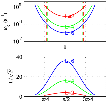
Figure 1: The parameter $\omega_{c}$ (with $B_{0}=0.31$ Gauss, $a=6.4\times 10^{8}$ cm, and $\rho_{e}=7$ amu $\mathrm{cm}^{-3}$), and the adiabatic growth/decay factor as a function of $\theta$ for various $L$ values of a dipole field. The vertical lines mark the location (colatitude) where $\omega_{c}=\omega_{0}$, the eigen-frequency of the corresponding fundamental mode.

As examples, the cases of a standard dipole field with a typical power-law density distribution have been examined for ULF waves in Earth’s magnetosphere (Webb et al., 2012) and coronal loop oscillations in Sun’s corona (Hu et al., 2012) by the above approach. Fig. 1 shows the variation of the cut-off frequency $\omega_{c}$ and the amplitude factor $f(\theta)$ for an axi-symmetric Earth’s dipole field, particularly for $L=2,4,6$ (here the value $L$ as in “$L$-shell” represents the radial distance of one particular field line crossing the equator). We use a density model by Kabin et al. (2007) throughout the present study: $\rho=\rho_{e}\left(\frac{r}{5}\right)^{4}$ with $\rho_{e}=7$ amu cm^-3 and the radial distance $r$ is measured in Earth radius. The general profiles of $\omega_{c}$ and $f$ are similar to those presented in Webb et al. (2012), but their magnitudes are sensitive to the different background density distributions assumed, as are the eigen-frequencies obtained. Table 1 lists the eigen-frequency of the fundamental mode $\omega_{0}$, the corresponding period $T_{0}$, and locations $\theta_{0}$ along each individual field line where $\omega_{0}=\omega_{c}(\theta_{0})$ for the dipole field. Given the profiles of $\omega_{c}(\theta)$ in Fig. 1, we find that for $\theta_{0}<\theta<\pi-\theta_{0}$ where $\omega>\omega_{c}$, the solution of the propagation type exists, while beyond that interval where $\omega<\omega_{c}$, decaying type solution exists, as reflected in the resulting wave forms from the corresponding eigen-function solutions (see Webb et al., 2012). The same set of results will be obtained for the case of a compressed dipole field in the following subsection.

2.2 A Compressed Dipole Field

A compressed dipole field is given in the spherical coordinate (which is intrinsically a 3D field, but remains planar at each $\phi$) (Kabin et al., 2007):

$$B_{r} = \left(\frac{2B_{0}}{r^{3}}-b_{1}(1+b_{2}\cos\phi)\right)\cos\theta,$$ (12)

$$B_{\theta} = \left(\frac{B_{0}}{r^{3}}+b_{1}(1+b_{2}\cos\phi)\right)\sin\theta,$$ (13)

$$B_{\phi} = 0.$$ (14)

So our approach can only be approximately applied to the noon-midnight meridional planes corresponding to $\phi=0$ and $\phi=\pi$ respectively, on which $\partial/\partial\phi=0$.

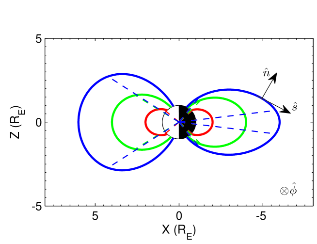
Figure 2: The magnetic field lines of $L=2,4,6$ on the noon-midnight meridional plane for the compressed dipole with $B_{0}=0.31$ Gauss, $b_{1}=10$ nT, and $b_{2}=8$. The dashed lines mark the locations where the eigen-frequencies of the fundamental mode intersect the cut-off frequencies, i.e., $\omega_{0}=\omega_{c}$ as shown in Fig. 3 and given in Tables 2 and 3. The field-line aligned orthogonal coordinate $(n,s,\phi)$ is also shown.

Fig. 2 shows the selected field lines for $L=2,4$, and 6, respectively, in both the noon ($\phi=0$) and midnight ($\phi=\pi$) meridional planes of the Earth as illustrated. The asymmetry between the two sides is clearly seen due to the compression of the solar wind on the noon side ($\mathrm{X}>0$). We carry out the analysis of toroidal mode waves for each individual field line via the approach of KG equations outlined in Section 2.1. The corresponding formulations of various coefficients, cut-off frequency and growth/decay amplitude factor for the compressed dipole geometry are given in the Appendix.

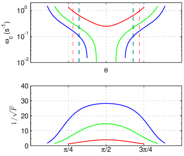
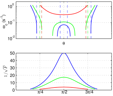
(a)                                                        (b)

Figure 3: The parameter $\omega_{c}$ (with $B_{0}=0.31$ Gauss, $a=6.4\times 10^{8}$ cm, and $\rho_{e}=7$ amu cm^-3), and the adiabatic growth/decay factor as a function of $\theta$ for various $L$ values for the compressed dipole field with (a) $\phi=0$ and (b) $\phi=\pi$, respectively. Format is the same as Fig. 1. The broken part of some curves corresponds to $\omega_{c}^{2}<0$.

First of all, the profiles of cut-off frequency $\omega_{c}$ and the amplitude factors are calculated and illustrated in Fig. 3, together with the locations where the eigen-frequencies of the fundamental mode intersect the cut-off frequencies. The corresponding parameters of the eigen-frequency $\omega_{0}$, the period $T_{0}$, the co-latitude $\theta_{0}$, and the radial distance $r_{0}$ where $\omega_{c}=\omega_{0}$ are given in Tables 2 and 3 for the noon and midnight side, respectively. The profiles of $\omega_{c}$ and $f$ show significant differences among the cases of noon, midnight meridional plane of the compressed dipole, and that of a standard dipole, especially for greater $L$ values. For example, for the case $L=6$ at midnight side, the amplitude factor peaks at a greater value $\sim 50$ at the equator, while the eigen-frequency $\omega_{0}$ intersects the cut-off frequency at two locations in $\theta<\pi/2$, one near the north pole and the other near the equator. Therefore there are two separate regions of propagating solution to the KG equation where $\omega^{2}>\omega_{c}^{2}$ and one additional region of evanescent solution surrounding the equator as marked by the pairs of dashed blue lines along congruent points in co-latitude. However for higher-order harmonics, the eigen-frequency increases with the increasing number of nodes such that it becomes greater than the cut-off frequency throughout the whole range of low latitudes enclosing the equator.

Overall, the values of parameters for the fundamental mode are comparable among the cases presented in Tables 1-3, although significant deviations also exist especially for the case of $L=6$. The periods range between a few to tens of seconds and a little over one-hundred seconds, with increasing $L$ values, which correspond well to the frequency range of Pc1-5 ULF waves in Earth’s magnetosphere. For the compressed dipole cases, the periods also agree well with those reported by Kabin et al. (2007), where the periods rose from a few seconds at $L=2$, to tens of seconds at $L=4$, and to $\sim 100$ seconds at $L=6$. The heights (radial distances) of the locations where $\omega_{c}=\omega_{0}$ increases with $L$ values, reaching much greater values in the compressed dipole case than that in the standard dipole. The corresponding co-latitudes, on the other hand, remain close to each other, except for the one near equator for $L=6$ in the midnight side of the compressed dipole case.

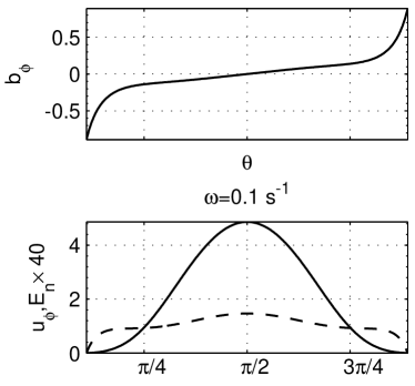
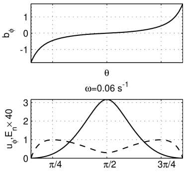
(a)                                                        (b)

Figure 4: Wave forms of the fundamental mode ($L=6$) on the (a) noon and (b) midnight meridional plane ($\phi=0$ and $\pi$), respectively. Dashed line denotes the electric field profile which is multiplied by 40. All units are arbitrary. The corresponding eigen-frequency is denoted in the middle of each subplot.

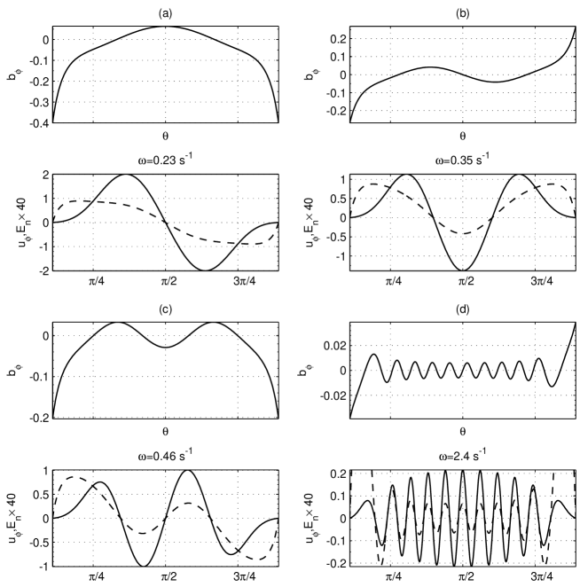
Figure 5: Harmonic wave forms (arbitrary unit) as derived from the solutions of the KG equation on the noon meridional plane ($\phi=0$) of the compressed dipole field for (a) n=1, (b) n=2, (c) n=3, and (d) n$>$4. Format is the same as Fig. 4.

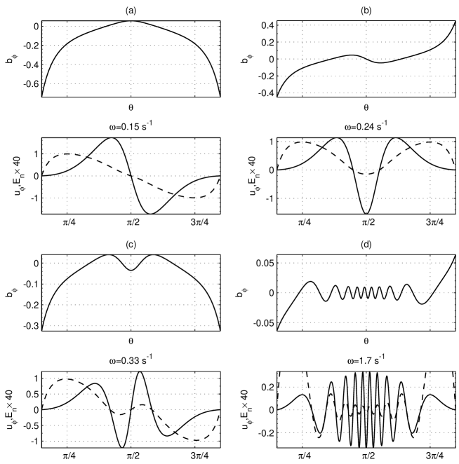
Figure 6: Harmonic wave forms on the midnight meridional plane ($\phi=\pi$) of the compressed dipole field. Format is the same as Fig. 5.

The choice of $L=6$, which shows the greatest asymmetry between the noon side and midnight side of the compressed dipole, is a representative case to illustrate the spatial wave forms as harmonic solutions to the KG equation. The number of nodes, n, contained in the solution of $u_{\phi}$ is increasing from 0 in the fundamental mode to consecutive positive integral numbers for higher-order harmonics. Fig. 4a, b show the fundamental modes for the noon and midnight side meridional planes of the compressed dipole. Similar to a standard dipole case (Webb et al., 2012), the $b_{\phi}$ profile contains one node at the equator, and the oscillating velocity $u_{\phi}$ and electric field $E_{n}$, normal to the background field (see Fig. 2) are in phase, given the boundary condition $E_{n}=0$ at both footpoints. The fundamental mode frequency at the midnight side is a little smaller than the noon side and the corresponding $E_{n}$ profile has a significant dip (much reduced amplitude) near the equator. These differences are caused by the different field-line geometry, the cut-off frequency and the amplitude factor for the two sides as discussed earlier. Such differences persist for higher-order harmonics. Figs. 5 and 6 show the wave forms of higher-order harmonics of increasing number of nodes on the noon and midnight side, respectively. The eigen-frequency increases with increasing number of nodes. The $u_{\phi}$ and $E_{n}$ perturbations remain in phase while the $b_{\phi}$ oscillation is generally out of phase by $\pi/2$. For the same harmonic mode, the midnight-side solution always has a smaller eigen-frequency and a smaller amplitude in $E_{n}$ around the equator.

3 Eigenvalue Solutions of the Poloidal Mode

In the poloidal mode, both the magnetic field and velocity perturbations of the waves are in the meridional plane. The normal components perpendicular to the field line (see Fig. 2) are denoted $b_{n}$ and $u_{n}$, respectively. Therefore, the only oscillating electric field is along the $\hat{\phi}$ direction, $E_{\phi}$, and after multiplied by a scaling factor, $\epsilon_{\phi}=r\sin\theta E_{\phi}$, is governed by (Cummings et al., 1969; Oliver et al., 1993; Lee and Takahashi, 2006)

$$\nabla^{2}\epsilon_{\phi}+2r\sin\theta\nabla\epsilon_{\phi}\cdot\nabla\left(\frac{1}{r\sin\theta}\right)+\frac{\omega^{2}}{V_{A}^{2}}\epsilon_{\phi}=0,$$ (15)

again assuming a harmonic time variation with angular eigen-frequency, $\omega$. The scaling factor $r\sin\theta$ arises from the curvilinear coordinate system other than a Cartesian geometry. In an equivalent cylindrical coordinate $(R,\phi,Z)$ ($\partial/\partial\phi=0$), it is written

$$\frac{\partial^{2}\epsilon_{\phi}}{\partial R^{2}}-\frac{1}{R}\frac{\partial\epsilon_{\phi}}{\partial R}+\frac{\partial^{2}\epsilon_{\phi}}{\partial Z^{2}}+\frac{\omega^{2}}{V_{A}^{2}}\epsilon_{\phi}=0.$$ (16)

In a Cartesian geometry, the differential operator in the above equation becomes a single Laplacian and $\epsilon_{\phi}\equiv E_{\phi}$ (e.g., Cummings et al., 1969). Here the Alfvén speed $V_{A}=B/\sqrt{\mu_{0}\rho}$ is again determined by a given background magnetic field and density model, and the equation is solved in a 2D domain such as a meridional plane of the compressed dipole field for $\phi=0$ and $\pi$ only. We are seeking eigen-mode solutions subject to boundary condition $\epsilon_{\phi}\equiv 0$ in the present study. Once the electric field perturbation is obtained, the magnetic field perturbations, $b_{r}$ and $b_{\theta}$, lying in the meridional plane, can be derived via Faraday’s law using the linear approximations.

Interestingly, the magnetic field perturbation normal to the field line, $b_{n}$, can be derived along each individual field line following the previous approach by the equation below which follows from the linearized Faraday’s law:

$$\frac{\partial{b_{n}}}{\partial t}=-\frac{B_{\theta}}{r^{2}B\sin\theta}\frac{d\epsilon_{\phi}}{d\theta}.$$ (17)

Note that the total derivative $d/d\theta$ here is evaluated along each individual field line and takes the form of Eq. (4). For harmonic oscillations, if we assign a phase lag of $\pi/2$ to $b_{n}$ relative to $E_{\phi}$ at initial time, the left-hand side of Eq. (17) becomes $\omega\tilde{b}_{n}$, which allows the derivation of a real-valued amplitude profile of $b_{n}$ based on solutions to Eq. (15). Similarly, the tangential component of the magnetic field perturbation is obtained by

$$\frac{\partial b_{s}}{\partial t}=\frac{1}{r\sin\theta}(\nabla\epsilon_{\phi}\cdot{\hat{n}})=\frac{1}{r\sin\theta}\left(-\frac{B_{r}}{rB}\frac{\partial\epsilon_{\phi}}{\partial\theta}+\frac{B_{\theta}}{B}\frac{\partial\epsilon_{\phi}}{\partial r}\right).$$ (18)

In general, the right-hand side of the above equation does not vanish, indicating a compressional fast mode solution. On the other hand, if it does vanish, i.e., $\partial\epsilon_{\phi}/\partial n=0$, a standing Alfvén wave mode should result. We separately analyze these two wave modes in the following subsections.

3.1 Poloidal Standing Transverse (Alfvén) Mode

This is a special case corresponding to $b_{s}\equiv 0$, i.e., $\partial\epsilon_{\phi}/\partial n=0$ from Eq. (18) above. This corresponds to a transverse, Alfvén mode of poloidal polarization of the magnetic field perturbation that is propagating along individual field lines. Therefore we can apply exactly the same approach of Section 2. The electric field perturbation $\epsilon_{\phi}$ still satisfies Eq. (15). However when applying the condition $b_{s}=0$ and projecting the PDE along an individual field line defined by a relation between $r$ and $\theta$, a wave equation of the form similar to Eq. (5) is obtained

$$\frac{\partial^{2}\epsilon_{\phi}}{\partial t^{2}}=\frac{V^{2}}{r^{2}}\left[\frac{d^{2}\epsilon_{\phi}}{d\theta^{2}}-\frac{d}{d\theta}\ln\left(\frac{B^{2}}{B_{\theta}^{2}}g(\theta)\sin\theta\right)\frac{d\epsilon_{\phi}}{d\theta}\right].$$ (19)

Here the wave speed parameter $V^{2}\equiv B^{2}_{\theta}/(\mu_{0}\rho)$ remains the same as before, and the function $g(\theta)$ is determined from a given background magnetic field model along an individual field line $r(\theta)$ by

$$\frac{d}{d\theta}\ln g(\theta)=\frac{B_{r}^{2}}{B_{\theta}^{2}}\frac{\partial}{\partial r}\left(\frac{rB_{\theta}}{B_{r}}\right).$$ (20)

For example, for a standard dipole field, the function $g(\theta)=\sin^{2}\theta$ is obtained.

Therefore the wave equation (19) can also be cast into a KG form and solved for eigenvalue solutions subject to the boundary condition $\epsilon_{\phi}=0$ at the footpoints of an individual field line. In turn the magnetic field perturbation can be derived from Eq. (17). Below we list the essential parameters for this mode conforming to the general descriptions in Section 2.1:

$$\frac{1}{L_{\epsilon}} = \frac{d}{d\theta}\ln\left(\frac{B^{2}}{B_{\theta}^{2}}g(\theta)\sin\theta\right)$$ (21)

$$\frac{1}{M_{\epsilon}} = 0,$$ (22)

and the amplitude factor

$$f(\theta)=\frac{B}{B_{\theta}}\sqrt{g(\theta)\sin\theta}.$$ (23)

For the dipole field, the following explicit formulas are obtained

$$f(\theta)=\sqrt{\sin\theta(1+3\cos^{2}\theta)}$$ (24)

$$\frac{1}{L_{\epsilon}}=\cot\theta-\frac{3\sin 2\theta}{1+3\cos^{2}\theta}.$$ (25)

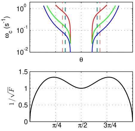
Figure 7: The parameters $\omega_{c}$ and $f(\theta)$ for the poloidal standing Alfvén waves of the dipole field. Format is the same as Fig. 1.

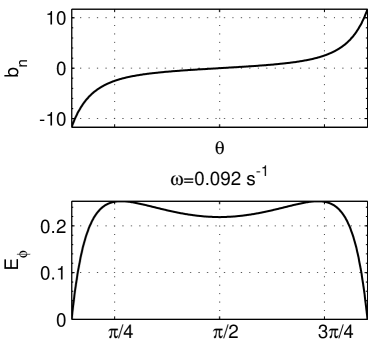
Figure 8: Wave forms (arbitrary unit) of the fundamental mode ($L=5$) for the poloidal standing Alfvén mode of the dipole field. Format is the same as Fig. 4.

Thus the cut-off frequency $\omega_{c}$ can be written based on Eq. (8). Fig. 7 shows, in the same format as before, the profiles of $\omega_{c}$ and $f$ for selected $L$ shells of the dipole field. Similarly the cut-off frequency exhibits minimum near the equator where $\omega_{c}^{2}$ becomes negative and increases toward the poles. The eigen-frequency of the fundamental mode generally intersects the cut-off frequency at low to mid latitudes. The solution of the KG equation would also be a combination of a propagation type near the equator and a decaying type near the two ends. The amplitude factor $f(\theta)$, on the other hand, shows much less variation in magnitude and does not depend on $L$. Fig. 8 shows the fundamental mode solutions for $L=5$, typical of a standing wave with zero number of node in electric field perturbation. The amplitude of $E_{\phi}$ dips slightly around the equator. The eigen-frequency is 0.092 s^-1, which corresponds to a period of 68s. It compares well with observations to be discussed below. Table 4 lists the corresponding parameters for the selected $L$ shells in the same format as Tables 1-3. The periods are in the same range as those of the toroidal mode.

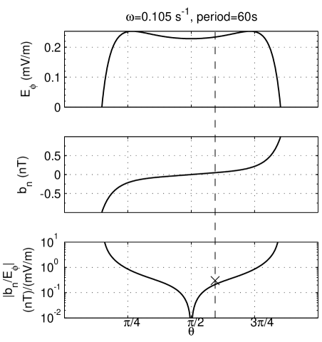
Figure 9: The solutions of $E_{\phi}$ (in mV/m), $b_{n}$ (in nT), and the ratio in-between (from top to bottom panels), to be compared with the spacecraft observations of Dai et al. (2013). The vertical dashed line denotes the spacecraft location and the cross sign marks the measured ratio ($\sim 0.3$ nT/(mV/m)) during the time period of measurements.

For a compressed dipole field, because the relation below $r$ and $\theta$ along a field line is implicit (see the Appendix), the relevant quantities have to be evaluated numerically. We leave detailed analysis of this particular case for future study. In what follows, we demonstrate the validity of our approach by comparing it with a most recent direct spacecraft observation of poloidal standing Alfvén waves by Dai et al. (2013). Fig. 9 shows our results of suitable physical units for $L=5$ of the dipole field with the same set of parameters as Dai et al. (2013), $\rho_{e}=6.4$ amu cm^-3 and the power index 1.0 of the density variation, to facilitate a direct comparison with their results (Fig. 3 therein). Dai et al. (2013) used a theoretical model of Cummings et al. (1969) and realistic ionosphere boundary conditions of finite conductivity at the footpoints of the field line. Therefore their solutions of $E_{\phi}$ and $b_{n}$ profiles are of finite values at the ends and are asymmetric about the equator whereas ours are symmetric and $E_{\phi}$ vanishes at the two ends. Nonetheless the spatial profiles over the low-mid latitudes still compare very well. The magnitudes of both perturbations show a slight decrease toward the equator in $E_{\phi}$ and rapid increase toward the ends in $b_{n}$. In particular, the ratio of $|b_{n}/E_{\phi}|$ at the spacecraft location ($\sim 17^{\circ}$ south in latitude), $\sim$ 0.21 nT/(mV/m), agrees well with their result, 0.25 nT/(mV/m), and the observed value, 0.3 nT/(mV/m). Similarly the period of the wave, 60s, compares well with 62s by Dai et al. (2013) and the observed value, 84s. Our result is also consistent with the observation in that $E_{\phi}$ leads the phase of $b_{n}$ by $\pi/2$ as discussed earlier.

3.2 Poloidal Compressional Mode

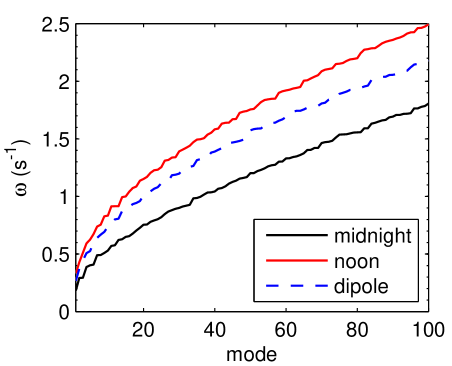
Figure 10: The first 100 eigen-frequencies for the noon side and midnight side of the compressed dipole, and a standard dipole field.

In the case that $b_{s}\neq 0$, Eq. (16) has to be solved in a two-dimensional domain as an eigenvalue problem subject to the boundary condition $E_{\phi}=0$ on all sides. As illustrative examples, we solve the equation and obtain the corresponding eigen-mode solutions of a discrete set of increasing eigen-frequencies by utilizing the software package PDE2D. The solutions are also cross-checked with the Matlab PDE toolbox and identical results are obtained. The computational domain is chosen as $r\in[1,L_{p}]R_{E}$, and $\theta\in[\theta_{p},\pi-\theta_{p}]$, where $\theta_{p}=\arcsin\sqrt{1/L_{p}}$. We choose $L_{p}=7$ in order to avoid the singular point in the compressed dipole field model as well as the singularity along the poles (X=0). We apply the dipole field and the compressed dipole field models and the same density distribution as before for the background field and plasma conditions. Three sets of eigen-frequencies of ascending order of magnitude (mode) are obtained for both the noon and midnight side meridional planes of the compressed dipole field and the standard dipole field. The first 100 eigen-frequencies are shown in Fig. 10. They generally exhibit a rapid rise at the lowest numbers of mode, then the trend of increase seems to become more gradual and eventually linear. At one specific mode, the eigen-frequency of the noon side is always greater than that of the midnight side, while the value of the dipole case is always in-between, albeit slightly closer to the value of the noon side.

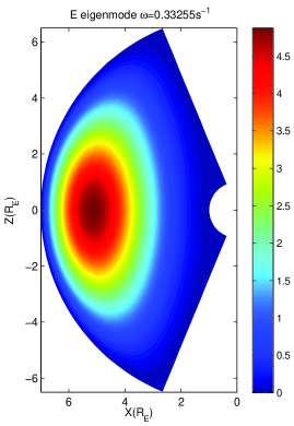
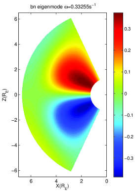
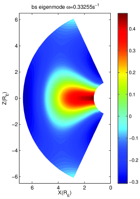
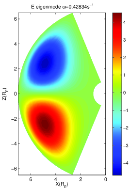
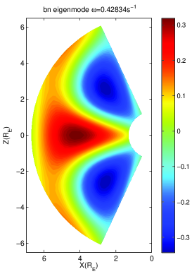
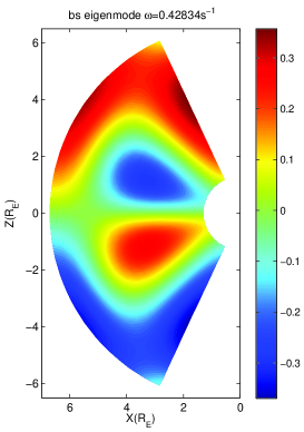
Figure 11: The fundamental (top row) and 1st-order harmonic (bottom row) eigen-mode solutions of $E_{\phi}$, $b_{n}$, and $b_{s}$ (from left to right columns) for $\phi=0$ (noon side) of the compressed dipole field. The corresponding eigen-frequencies are indicated on top of each panel. The scales (all of arbitrary units) are given by the colorbars.

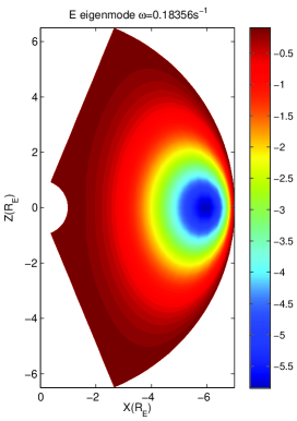
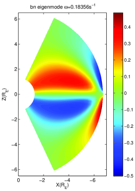
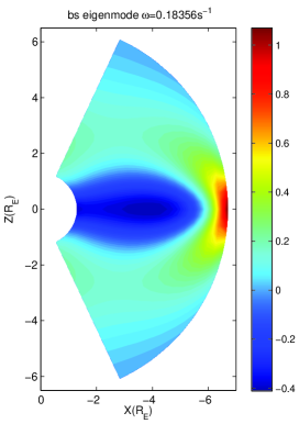
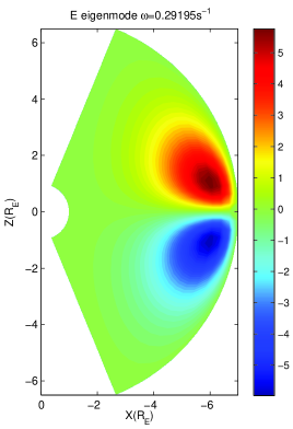
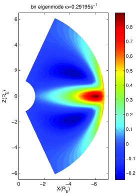
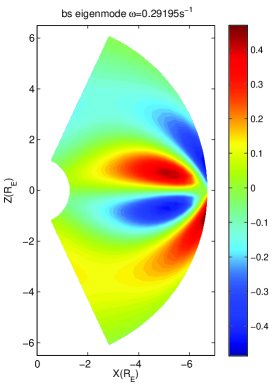
Figure 12: The eigen-mode solutions for $\phi=\pi$ (midnight side) of the compressed dipole field. Format is the same as Fig. 11.

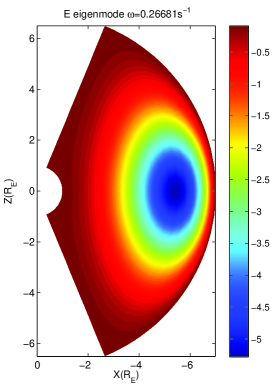
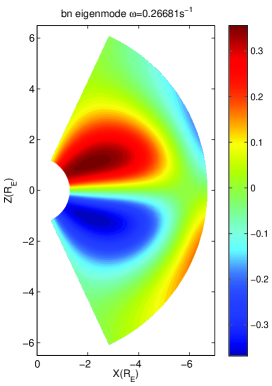
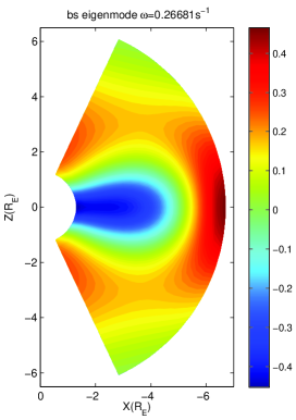
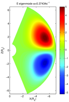
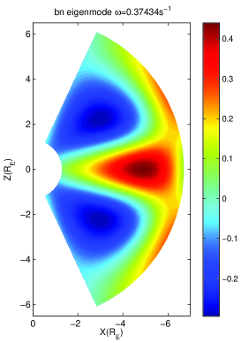
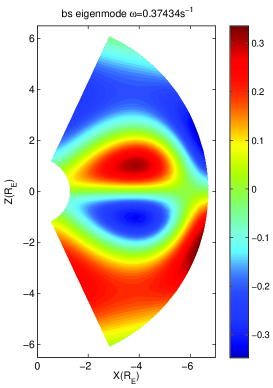
Figure 13: The eigen-mode solutions of the dipole field. Format is the same as Fig. 11.

In Figs. 11-13, we show the corresponding eigen-mode solutions of the two lowest-value eigen-frequencies for the noon, midnight side of the compressed dipole field, and the standard dipole field, respectively. The solutions generally display a regular pattern of nodal structures, especially in higher-order mode solutions of progressively larger eigen-frequencies (not shown). Starting from the lowest-order mode, the number of nodes between adjacent extreme values increases by 1, especially in the $\theta$ direction and sometimes in the $r$ direction as well. The “peaks” and “valleys” are alternating in appearances as deep red and deep blue patches. The number of nodes in the normal magnetic field perturbation $b_{n}$ is usually increased by one compared with the corresponding electric field perturbation $E_{\phi}$. However the number of nodes in the tangential magnetic field perturbation $b_{s}$ remains the same as that of $E_{\phi}$, albeit the overall shape of the distribution is much different. Therefore in the fundamental mode solutions, the normal magnetic field perturbation (representative of the radial component) exhibits a two-lobe structure in amplitude symmetric about the equator, especially in the mid-range radial distances, excluding the boundary effect. The tangential component (parallel to the background magnetic field), on the other hand, shows a single-lobe structure peaking at the equator. These results are qualitatively similar to those shown by Lee and Takahashi (2006), where much more sophisticated numerical approaches, and more realistic background density distribution and boundary conditions were utilized. Our preliminary numerical experiments also indicate that the background magnetic field greatly affects the eigenvalue solutions. For example, the overall behavior of the solutions of the noon-side compressed dipole is very similar to that of the standard dipole since their magnetic field topologies are close to each other. However for the midnight-side compressed dipole, the locations of the extreme values are generally further stretched to larger radial distances anti-sunward and the shapes are narrower.

4 Conclusions and Discussion

In conclusion, we have examined, in a fairly comprehensive manner, the decoupled toroidal and poloidal mode hydromagnetic waves in cold plasmas (ULF waves) with applications to the Earth’s inner magnetosphere, represented by a compressed dipole field model in addition to the standard dipole field. Under certain assumptions, the decoupled wave equations are recast into the Klein-Gordon (KG) form along individual magnetic field lines, especially for both the toroidal and poloidal transverse Alfvén waves. We obtain the spatial profiles of the characteristic parameters in the KG formulations including the cut-off frequency $\omega_{c}$ and the amplitude factor $f$. The former determines the property of the solution, i.e., whether it is a propagation type where the eigen-frequency $\omega>\omega_{c}$ usually occurring near the equator or an evanescent type where $\omega<\omega_{c}$ toward the footpoints. The latter modulates the amplitude of the wave forms spatially. We obtain the sets of eigenvalue solutions of increasing eigen-frequencies and number of nodes in the wave forms for different background magnetic field geometries. The corresponding wave periods are in the order of $\sim 1$ second to $\sim 100$ seconds and compare well quantitatively with prior studies and observations. In particular, we present a case study of a fundamental poloidal Alfvén wave via our approach and compare our results with a direct spacecraft observation by Dai et al. (2013). The wave period ($\sim 60$s) and the amplitude ratio ($\sim$ 0.21 nT/(mV/m)) obtained from our approach agree well with the spacecraft measurements (84s and 0.3 nT/(mV/m), respectively) and the results from the other approach. For completeness, we also carry out preliminary numerical computations of the eigen-mode solutions to the compressional poloidal waves where the tangential magnetic field perturbation does not vanish. Qualitatively consistent results with prior studies are obtained.

We acknowledge that the present investigations reported here have largely been studied in many prior works. The main intellectual merits thus lie in the aspect of the unique approach via the KG equations for both the toroidal and poloidal transverse Alfvén waves for a given background magnetic field geometry. The implications of our results, for example, that of the cut-off frequency, need to be further explored. In particular, the case study of a direct comparison with spacecraft measurements yields promising results, despite the relatively simple and idealized assumptions about the axi-symmetric geometry and boundary conditions. It is worth persuing beyond the limitations of the present approach, especially in conjunction with the state-of-the-art spacecraft observations, such as those returned from the Van Allen Probe. Furthermore, it is also desirable to extend the applications to the solar coronal loop oscillations as we did in Hu et al. (2012).

Table 1: List of parameters for $L=2,4,6$ of a standard dipole field.

$L$	$\omega_{0}$, s-1	$T_{0}$, s	$\theta_{0}$, ∘	$r_{0}$, $R_{E}$
2	0.95	6.6	49	1.15
4	0.20	32	52	2.48
6	0.085	74	53	3.81

Table 2: List of parameters for $L=2,4,6$ of a compressed dipole field for $\phi=0$ (noon).

$L$	$\omega_{0}$, s-1	$T_{0}$, s	$\theta_{0}$, ∘	$r_{0}$, $R_{E}$
2	0.96	6.6	50	1.20
4	0.22	29	58	3.06
6	0.10	60	57	5.05

Table 3: List of parameters for $L=2,4,6$ of a compressed dipole field for $\phi=\pi$ (midnight).

$L$	$\omega_{0}$, s-1	$T_{0}$, s	$\theta_{0}$, ∘	$r_{0}$, $R_{E}$
2	0.94	6.7	48	1.11
4	0.18	34	45	1.86
6	0.060	105	83 (39)	5.81 (1.90)

Table 4: List of parameters for $L=2,4,6$ of a dipole field for poloidal standing Alfvén waves.

$L$	$\omega_{0}$, s-1	$T_{0}$, s	$\theta_{0}$, ∘	$r_{0}$, $R_{E}$
2	0.76	8.2	57	1.41
4	0.15	42	62	3.09
6	0.062	101	62	4.71

Appendix A KG Formulations for a Compressed Dipole Field

In this section, we provide the necessary formulations of the KG equations for a compressed dipole field in a spherical coordinates with the magnetic field components given by Eqs. (12) to (14).

Since the field remains planar (i.e., $B_{\phi}=0$), it is possible to derive the field line equation in each meridional plane ($r$, $\theta$, $\phi\equiv Const$) with $r$ normalized by Earth radius:

$$\frac{dr}{d\theta}=\frac{rB_{r}}{B_{\theta}}=\frac{r(2/r^{3}-D)}{1/r^{3}+D}\cot\theta,$$ (26)

where $D\equiv\frac{b_{1}}{B_{0}}(1+b_{2}\cos\phi)$. This leads to

$$H\sin^{2}\theta=\frac{r}{D\cdot r^{3}-2},$$ (27)

where $H$ is an integration constant. As usual, if we define $r=L$ when $\theta=\pi/2$ ($L$-shell), we obtain $H=L/(D\cdot L^{3}-2)$. Then the co-latitude $\theta_{F}$ of one of the footpoints of one particular $L$-shell is obtained by $\sin^{2}\theta_{F}=1/(H\cdot D-2H)$.

Subsequently, the necessary coefficients and factor in the KG equation for the velocity perturbation in the toroidal mode are obtained as follows

$$\frac{1}{l_{u}} = -\frac{1}{l_{b}}=\frac{3}{1+D\cdot r^{3}}\cot\theta$$ (28)

$$\frac{1}{L_{u}} = \frac{7-4D\cdot r^{3}-2D^{2}r^{6}}{(1+D\cdot r^{3})^{2}}\cot\theta.$$ (29)

Additional coefficients such as $1/M_{u}$ can be derived according to Webb et al. (2012) which enables the derivation of an analytic form of the cut-off frequency $\omega_{c}$ appearing in the KG equation and the amplitude factor $f(\theta)$, relating the solution of KG equation to the original physical perturbation quantity.

For the poloidal mode, the analytic formulae for the relevant factors in the corresponding KG equation have to be evaluated numerically since an explicit form of the function $g(\theta)$ from Eq. (20) along an individual field line is difficult to obtain.

References

- Claudepierre et al. (2010) Claudepierre, S. G., Hudson, M. K., Lotko, W., Lyon, J. G., Denton, R. E., Nov. 2010. Solar wind driving of magnetospheric ULF waves: Field line resonances driven by dynamic pressure fluctuations. Journal of Geophysical Research (Space Physics) 115, 11202.
- Cummings et al. (1969) Cummings, W. D., O’Sullivan, R. J., Coleman, Jr., P. J., 1969. Standing Alfvén waves in the magnetosphere. J. Geophys. Res.74, 778.
- Dai et al. (2013) Dai, L., Takahashi, K., Wygant, J. R., Chen, L., Bonnell, J., Cattell, C. A., Thaller, S., Kletzing, C., Smith, C. W., MacDowall, R. J., Baker, D. N., Blake, J. B., Fennell, J., Claudepierre, S., Funsten, H. O., Reeves, G. D., Spence, H. E., Aug. 2013. Excitation of poloidal standing Alfvén waves through drift resonance wave-particle interaction. Geophys. Res. Lett.40, 4127–4132.
- Elkington (2006) Elkington, S. R., 2006. A Review of ULF Interactions With Radiation Belt Electrons. In: Takahashi, K., Chi, P. J., Denton, R. E., Lysak, R. L. (Eds.), Magnetospheric ULF Waves: Synthesis and New Directions. Vol. 169 of Washington DC American Geophysical Union Geophysical Monograph Series. p. 177.
- Elkington et al. (1999) Elkington, S. R., Hudson, M. K., Chan, A. A., 1999. Acceleration of relativistic electrons via drift-resonant interaction with toroidal-mode Pc-5 ULF oscillations. Geophys. Res. Lett.26, 3273–3276.
- Elkington et al. (2003) Elkington, S. R., Hudson, M. K., Chan, A. A., Mar. 2003. Resonant acceleration and diffusion of outer zone electrons in an asymmetric geomagnetic field. Journal of Geophysical Research (Space Physics) 108, 1116.
- Fraser (2006) Fraser, B. J., 2006. ULF Waves-A Historical Note. In: Takahashi, K., Chi, P. J., Denton, R. E., Lysak, R. L. (Eds.), Magnetospheric ULF Waves: Synthesis and New Directions. Vol. 169 of Washington DC American Geophysical Union Geophysical Monograph Series. p. 5.
- Hu et al. (2012) Hu, Q., McKenzie, J. F., Webb, G. M., May 2012. Klein-Gordon equations for horizontal transverse oscillations in two-dimensional coronal loops. Astron. Astrophys.541, A53.
- Kabin et al. (2007) Kabin, K., Rankin, R., Mann, I. R., Degeling, A. W., Marchand, R., Mar. 2007. Polarization properties of standing shear Alfvén waves in non-axisymmetric background magnetic fields. Annales Geophysicae 25, 815–822.
- Kivelson (2006) Kivelson, M. G., 2006. ULF waves from the ionosphere to the outer planets. In: Takahashi, K., Chi, P. J., Denton, R. E., Lysak, R. L. (Eds.), Magnetospheric ULF Waves: Synthesis and New Directions. Vol. 169 of Washington DC American Geophysical Union Geophysical Monograph Series. pp. 11–30.
- Lee and Takahashi (2006) Lee, D.-H., Takahashi, K., 2006. MHD Eigenmodes in the Inner Magnetosphere. In: Takahashi, K., Chi, P. J., Denton, R. E., Lysak, R. L. (Eds.), Magnetospheric ULF Waves: Synthesis and New Directions. Vol. 169 of Washington DC American Geophysical Union Geophysical Monograph Series. p. 73.
- Liu et al. (2013) Liu, W., Cao, J. B., Li, X., Sarris, T. E., Zong, Q.-G., Hartinger, M., Takahashi, K., Zhang, H., Shi, Q. Q., Angelopoulos, V., Jul. 2013. Poloidal ULF wave observed in the plasmasphere boundary layer. Journal of Geophysical Research (Space Physics) 118, 4298–4307.
- Liu et al. (2011) Liu, W., Sarris, T. E., Li, X., Zong, Q.-G., Ergun, R., Angelopoulos, V., Glassmeier, K. H., Oct. 2011. Spatial structure and temporal evolution of a dayside poloidal ULF wave event. Geophys. Res. Lett.38, 19104.
- McKenzie and Hu (2010) McKenzie, J. F., Hu, Q., Mar. 2010. Klein-Gordon equations for toroidal hydromagnetic waves in an axi-symmetric field. Annales Geophysicae 28, 737–742.
- Oliver et al. (1993) Oliver, R., Ballester, J. L., Hood, A. W., Priest, E. R., Jun. 1993. Magnetohydrodynamic waves in a potential coronal arcade. Astronomy and Astrophysics 273, 647.
- Singer et al. (1981) Singer, H. J., Southwood, D. J., Walker, R. J., Kivelson, M. G., Jun. 1981. Alfven wave resonances in a realistic magnetospheric magnetic field geometry. J. Geophys. Res.86, 4589–4596.
- Southwood and Hughes (1983) Southwood, D. J., Hughes, W. J., 1983. Theory of hydromagnetic waves in the magnetosphere. Space Sci. Rev.35, 301–366.
- Takahashi et al. (2002) Takahashi, K., Denton, R. E., Gallagher, D., Feb. 2002. Toroidal wave frequency at L = 6-10: Active Magnetospheric Particle Tracer Explorers/CCE observations and comparison with theoretical model. Journal of Geophysical Research (Space Physics) 107, 1020.
- Takahashi et al. (2013) Takahashi, K., Hartinger, M. D., Angelopoulos, V., Glassmeier, K.-H., Singer, H. J., Jul. 2013. Multispacecraft observations of fundamental poloidal waves without ground magnetic signatures. Journal of Geophysical Research (Space Physics) 118, 4319–4334.
- Tamao (1965) Tamao, T., Jun. 1965. Transmission and coupling resonance of hydromagnetic disturbances in the non-uniform Earth’s magnetosphere. Sci. Rep. Tohoku Univ., Ser. 5, Geophys. 17, 43–72.
- Ukhorskiy et al. (2005) Ukhorskiy, A. Y., Takahashi, K., Anderson, B. J., Korth, H., Oct. 2005. Impact of toroidal ULF waves on the outer radiation belt electrons. Journal of Geophysical Research (Space Physics) 110, 10202.
- Volwerk (2006) Volwerk, M., 2006. Multi-Satellite Observations of ULF Waves. In: Takahashi, K., Chi, P. J., Denton, R. E., Lysak, R. L. (Eds.), Magnetospheric ULF Waves: Synthesis and New Directions. Vol. 169 of Washington DC American Geophysical Union Geophysical Monograph Series. p. 109.
- Webb et al. (2012) Webb, G. M., McKenzie, J. F., Hu, Q., Zank, G. P., May 2012. Toroidal hydromagnetic waves in an axi-symmetric magnetic field. Journal of Geophysical Research (Space Physics) 117, 5229.
(a) (b)
(a) (b)