Many-body theory of the neutralization of strontium ions on gold surfaces

Abstract

Motivated by experimental evidence for mixed-valence correlations affecting the neutralization of strontium ions on gold surfaces we set up an Anderson-Newns model for the Sr:Au system and calculate the neutralization probability $\alpha$ as a function of temperature. We employ quantum-kinetic equations for the projectile Green functions in the finite$-U$ non-crossing approximation. Our results for $\alpha$ agree reasonably well with the experimental data as far as the overall order of magnitude is concerned showing in particular the correlation-induced enhancement of $\alpha$. The experimentally found non-monotonous temperature dependence, however, could not be reproduced. Instead of an initially increasing and then decreasing $\alpha$ we find over the whole temperature range only a weak negative temperature dependence. It arises however clearly from a mixed-valence resonance in the projectile’s spectral density and thus supports qualitatively the interpretation of the experimental data in terms of a mixed-valence scenario.

I Introduction

Charge-transferring atom-surface collisions Monreal (2014); Winter and Burgdörfer (2007); Winter (2002); Rabalais (1994); Los and Geerlings (1990); Brako and Newns (1989); Modinos (1987); Yoshimori and Makoshi (1986); Newns et al. (1983) are of great technological interest in surface science. The complex process of neutral gas heating in fusion plasmas, Kraus et al. (2007) for instance, starts with the surface-based conversion of neutral hydrogen atoms to negatively charged ions. The operation modii of low-temperature plasmas used, for instance, in flat panel displays or in surface modification devices depend strongly on secondary electrons originating from the substrate due to impact of ions and radicals and thus also on surface-based charge-transfer processes. Lieberman and Lichtenberg (2005) Many surface diagnostics, finally, for instance, ion neutralization spectroscopy Rabalais (2003) and meta-stable atom de-excitation spectroscopy Harada et al. (1997) utilize charge-transfer processes to gain information about the constituents of the surface. At the same time, however, charge-transferring atom-surface collisions are of fundamental interest as well because they are particular realizations of a quantum-impurity system out of equilibrium.

The archetypical quantum-impurity is a local spin (more generally, a local moment) in a metal coupled to the itinerant electrons of the conduction band. Its well-documented properties, Hewson (1993); Fulde (1995) arising from an emerging resonance at the Fermi energy of the metal, are however also present in other quantum systems with a finite number of correlated internal states interacting via tunneling with a reservoir of external states. In particular, semiconductor quantum-dots coupled to metallic leads are ideal platforms for studying local-moment physics in a well-controlled setting. Chang and Chen (2009); Pustilnik and Glazman (2004); Aguado and Langreth (2003); Goldhaber-Gordon et al. (1998a); Cronenwett et al. (1998); Goldhaber-Gordon et al. (1998b); Wingreen and Meir (1994); Grabert and Devoret (1992) By a suitable time-dependent gating the dot can be driven out of equilibrium. Of particular recent theoretical interest are the temporal build-up and/or decay of local-moment-type correlations and how they affect the electron transport through these devices. Nghiem and Costi (2014); Lechtenberg and Anders (2014); Mühlbacher et al. (2011); Cohen and Rabani (2011) As pointed out a long time ago by Shao and coworkers Shao et al. (1996) as well as Merino and Marston Merino and Marston (1998), similar transient correlations should also occur in charge-transferring atom-surface collisions where the projectile with its finite number of electron states mimics the quantum dot while the target with its continuum of states replaces the lead.

A recent experiment by He and Yarmoff indeed provided strong evidence for local-moment-type correlations to affect the neutralization probability of strontium ions on gold surfaces. He and Yarmoff (2011, 2010) They found a non-monotonous temperature dependence of the neutralization probability which first increases and then decreases with temperature. The initial increase with temperature is most probably a thermal single-particle effect but the latter could be the long-sought fingerprint for a transient mixed-valence resonance formed during an electron-transfer from a surface to an atomic projectile. Shao et al. (1996); Merino and Marston (1998)

In the present work, following the lead of Nordlander and coworkers Shao et al. (1996, 1994a, 1994b); Langreth and Nordlander (1991) as well as Merino and Marston, Merino and Marston (1998) we analyze He and Yarmoff’s experiment He and Yarmoff (2011, 2010) from a many-body theoretical point of view. In particular we test the claim that the negative temperature dependence at high temperatures arises from the local moment of the unpaired electron in the $5s$ shell of the approaching ion. For that purpose we first set up, as usual for the description of charge-transferring atom-surface collisions, an Anderson-Newns Hamiltonian. Los and Geerlings (1990); Brako and Newns (1989); Modinos (1987); Yoshimori and Makoshi (1986); Kasai and Okiji (1987); Nakanishi et al. (1988); Newns et al. (1983); Romero et al. (2009); Bajales et al. (2007); Goldberg et al. (2005); Onufriev and Marston (1996); Marston et al. (1993) To obtain its single-particle matrix elements we employ Hartree-Fock wave functions for the strontium projectile, Clementi and Roetti (1974) a step-potential description for the gold target, and Gadzuk’s semi-empirical construction Gadzuk (1967a, b, 2009) for the projectile-target interaction. The model rewritten in terms of Coleman’s pseudo-particle operators Coleman (1984); Kotliar and Ruckenstein (1986) is then analyzed within the finite$-U$ non-crossing approximation employing contour-ordered Green functions Kadanoff and Baym (1962); Keldysh (1965) as originally suggested by Nordlander and coworkers. Shao et al. (1996, 1994a, 1994b); Langreth and Nordlander (1991) Besides the instantaneous occupancies and the neutralization probability we also calculate the instantaneous spectral densities. The latter are of particular interest because if the interpretation of the experimental findings in terms of a mixed-valence scenario is correct, the projectile’s spectral density should feature a transient resonance at the target’s Fermi energy.

For the material parameters best suited for the Sr:Au system we find neutralization probabilities slightly above the experimental data but still of the correct order of magnitude indicating that the single-particle matrix elements of the Anderson-Newns model are sufficiently close to reality. Moreover, for the model without correlations the neutralization probabilities turn out to be too small showing that agreement with experiment can be only achieved due to the correlation-induced enhancement of the neutralization probability. We also find a transient resonance in the instantaneous spectral densities hinting mixed-valence correlations to be present in certain parts of the collision trajectory. The non-monotonous temperature dependence of the neutralization probability, however, could not be reproduced. Instead we find the resonance to lead only to a weak negative temperature dependence over the whole temperature range.

Due to lack of data for comparison we cannot judge the validity of the single-particle parameterization we developed for the Sr:Au system. At the moment it is the most realistic one. We attribute therefore the failure of the present calculation to reproduce the temperature anomaly of the neutralization probability while having at the same time mixed-valence features in the instantaneous spectral densities primarily to the finite$-U$ non-crossing approximation which seems to be unable to capture the instantaneous energy scales with the required precision. A quantitative description of the experiment has thus to be based either on the dynamical $1/N$ expansion initially used by Merino and Marston, Merino and Marston (1998) equation of motions for the correlation functions of the physical degrees of freedom instead of the pseudo-particles, Goldberg et al. (2005) or on the one-crossing approximation as it has been developed for the equilibrium Kondo effect. Otsuki and Kuramoto (2006); Kroha and Wölfle (2005); Pruschke and Grewe (1989); Holm and Schönhammer (1989); Sakai et al. (1988) Numerically this will be rather demanding. But demonstrating that He and Yarmoff have–for the first time–indeed seen local-moment physics in a charge-transferring atom-surface collision may well be worth the effort.

The paper is organized as follows. In the next section we introduce the Anderson-Newns model, its parameterization for the Sr:Au system, and its representation in terms of pseudo-particle operators. In Sec. III we recapitulate briefly the quantum kinetics of the Anderson-Newns model as pioneered by Nordlander and coworkers. Basic definitions and the main steps of the derivation of the set of Dyson equations for the analytic pieces of the projectile Green functions within the finite-$U$ non-crossing approximation, which is the set of equations to be numerically solved, can be found in an appendix to make the paper self-contained. Numerical results are presented, discussed, and compared to the experimental data in Sec. IV and concluding remarks with an outlook are given in Sec. V.

II Model

The interaction of an atomic projectile with a surface is a complicated many-body process. Within the adiabatic approximation, which treats the center-of-mass motion of the projectile along the collision trajectory classically, Yoshimori and Makoshi (1986) it leads to a position- and hence time-dependent broadening and shifting of the projectile’s energy levels. The adiabatic modification of the atomic energy levels as a function of distance can be calculated from first principles. Nordlander and Tully (1988, 1990); Borisov and Wille (1995); More et al. (1998); Valdés et al. (2005) As in our previous work on secondary electron emission from metallic Marbach et al. (2012a) and dielectric Marbach et al. (2012b); Marbach et al. (2011) surfaces, we employ however Gadzuk’s semi-empirical approach Gadzuk (1967a, b)–based on classical image shifts and a golden rule calculation of the level widths–which not only provides a very appealing physical picture of the interaction process Gadzuk (2009) but produces for distances larger than a few Bohr radii also reasonable level widths and shifts. Borisov and Wille (1995); More et al. (1998); Valdés et al. (2005)

Indeed, first-principle investigations of Auger neutralization of helium ions on aluminum surfaces by Monreal and coworkers More et al. (1998); Valdés et al. (2005) showed that for distances larger than five Bohr radii the level shift follows the classical image shift. Only for shorter distances chemical interactions lead to a substantial deviation between the two. Borisov and Wille, Borisov and Wille (1995) on the other hand, found the level width of hydrogen ions approaching an aluminum surface to be for distances larger than five Bohr radii also not too far off the widths obtained from Gadzuk’s golden rule calculation, that is, the widths are perhaps off by a factor two. The reason most probably is Gadzuk’s ingenious choice of the tunneling matrix element (see below) which takes care of the non-orthogonality of the projectile and target states. Gadzuk (1967b) Since the turning point of the strontium ion is sufficiently far away from the first atomic layer, we estimate it to be around five Bohr radii, we expect Gadzuk’s semi-empirical approach to also provide a reasonable parameterization of the Sr:Au system investigated by He and Yarmoff. He and Yarmoff (2010, 2011) The corrections due to chemical interactions between the strontium projectile and the gold surface, occurring at shorter distances and included in first-principle approaches, Nordlander and Tully (1988, 1990); Borisov and Wille (1995); More et al. (1998); Valdés et al. (2005) should not yet play a role.

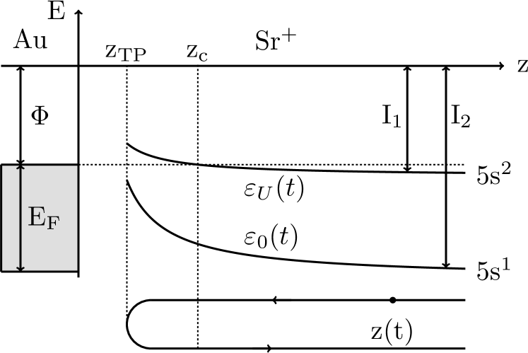
Figure 1: Illustration of the time-dependent charge-transferring scattering of a $\mathrm{Sr^{+}}$ ion on a gold surface. Far from the surface the two ionization energies $\varepsilon_{0}(t)$ and $\varepsilon_{U}(t)$ are equal to the first two ionization energies of a strontium atom and represent the projectile’s $\mathrm{5s^{1}}$ and $\mathrm{5s^{2}}$ configuration. They shift upward due to the image interaction of the projectile with the surface. For simplicity not shown is the hybridization between the projectile and surface states as the projectile closes its distance to the surface which is idealized by a step-potential whose depth is the sum of the work function $\Phi>0$ and the Fermi energy $E_{F}>0$. The energies are on scale and the points indicated along the trajectory $z(t)$ are $z_{\rm TP}$, the turning point, and $z_{c}$, the point where the first ionization level crosses the Fermi energy.

We now set up Gadzuk’s approach step by step. Gadzuk (1967a, b) For the charge-transfer process we are interested in, the first two ionization levels of the strontium projectile are most important. They are closest to the Fermi energy of the gold target and may hence accept or donate an electron. In terms of the Anderson-Newns model, the two levels constitute, respectively, the upper and lower charge-transfer level. The difference of the two can thus be identified with the time-dependent on-site Coulomb repulsion. Figure 1 schematically shows the essence of the Anderson-Newns model for the Sr:Au system. The energy levels are on scale. Mathematically, the on-site energies are given by

$$\varepsilon_{U}(t) =-I_{1}+\dfrac{e^{2}}{4\left|z(t)-z_{i}\right|}~{},$$ (1)

$$\varepsilon_{0}(t) =-I_{2}+\dfrac{3e^{2}}{4\left|z(t)-z_{i}\right|}~{},$$ (2)

where $I_{1}>0$ and $I_{2}>0$ are the first and second ionization energies far from the surface and $z_{i}$ is the distance of the metal’s image plane from its crystallographic ending at $z=0$. For simplicity the projectile is assumed to approach the surface perpendicularly along the trajectory,

$$z(t)=z_{\rm TP}+v\left|t\right|~{},$$ (3)

where $z_{\rm TP}$ is the turning point and $v$ is the velocity.

The shift of the on-site energies with time can be interpreted as the negative of the energy gain of a virtual process which moves the configuration under consideration from the actual position $z$ to $z=\infty$, reduces its electron occupancy by one, and then moves it back to its former position $z$, taking into account in both moves possible image interactions due to the initial and final charge-state of the projectile with the metal. Newns et al. (1983)

For the upper level, $\varepsilon_{U}(z)$, corresponding to the first ionization level, this means shifting the charge-neutral $5s^{2}$ configuration from $z$ to $z=\infty$, turning it into a single-charged $5s^{1}$ configuration, which is then moved back to $z$. In the first leg no image shift occurs while in the second one the image shift is $-e^{2}/4|z-z_{i}|$. The net energy gain of the whole process is therefore $-e^{2}/4|z-z_{i}|$ leading to a shift of the upper on-site level of $+e^{2}/4|z-z_{i}|$. Similarly, for the lower level, $\varepsilon_{0}(z)$, which is the second ionization level, one imagines moving a $5s^{1}$ configuration from $z$ to $z=\infty$ and then a $5s^{0}$ configuration from $z=\infty$ back to $z$. In both moves image shifts occur adding up to $-3e^{2}/4|z-z_{i}|$ because the energy pay in the first half of the trip is due to a single-charged projectile while the energy gain on the return trip arises from a double-charged one. The shift of the lower on-site level is thus $+3e^{2}/4|z-z_{i}|$.

	$I_{1}$[eV]	$Z_{1}$	$I_{2}$[eV]	$Z_{2}$	$\Phi$[eV]	$E_{F}$[eV]	$z_{\rm i}$[a.u.]	$m_{e}^{*}/m_{e}$
Sr	5.7	1.65	11.0	2	–	–	–	–
Au	–	–	–	–	5.1	5.53	1.0	1.1

Table 1: Material parameters for strontium and gold: $I_{1}$ and $I_{2}$ are the first and the second ionization energy, $Z_{1}$ and $Z_{2}$ are the effective charges to be used in the calculation of the hybridization matrix element (viz: Eq. (8)), $\Phi$ is the work function, $E_{F}$ the Fermi energy, $z_{i}$ the position of the image plane in front of the surface for which we take a typical value, and $m_{e}^{*}$ is the effective mass of an electron in the conduction band of gold.

Besides the on-site energies we also need the hybridization matrix elements which depend on projectile and metal wave functions. Ignoring the lateral variation of the surface potential, we take for the latter simply the wave functions of a step potential with depth $V_{0}=-\Phi-E_{F}$ where $\Phi>0$ and $E_{F}>0$ are the work function and the Fermi energy of the surface, respectively, measured as illustrated in Fig. 1. Hence, the energies and wave functions for the conduction band electrons are

$$\varepsilon_{\vec{k}} =\frac{\hbar^{2}}{2m^{*}_{e}}\left(k_{x}^{2}+k_{y}^{2}+k_{z}^{2}\right)-\left|V_{0}\right|~{},$$ (4)

$$\psi_{\vec{k}}(\vec{r}) =\dfrac{1}{L^{3/2}}e^{i(k_{x}x+k_{y}y)}\Bigl{\{}\Theta(z)T_{k_{z}}e^{-\kappa_{z}z}$$

$$+\Theta(-z)\left[e^{ik_{z}z}+R_{k_{z}}e^{-ik_{z}z}\right]\Bigr{\}}~{},$$ (5)

where $L$ is the spatial width of the step, which drops out in the final expressions, and

$$T_{k_{z}}=\frac{2ik_{z}}{ik_{z}-\kappa_{z}}~{},~{}~{}R_{k_{z}}=\frac{ik_{z}+\kappa_{z}}{ik_{z}-\kappa_{z}}~{},$$ (6)

with $\kappa_{z}=\sqrt{2m_{e}(\left|V_{0}\right|-k_{z}^{2})/\hbar^{2}}$ are, respectively, the transmission and reflection coefficients of the step potential. More sophisticated surface potentials are conceivable but from the work of Kürpick and Thumm Kürpick and Thumm (1996) we expect the final result for the neutralization probability to depend not too strongly on the choice of the surface potential.

For the calculation of the hybridization matrix element we also need $5s$ wave functions for the neutral and single-charged projectile. Both are radially symmetric and in the Hartree-Fock approximation can be written in the general form

$$\psi_{\rm{HF}}(\vec{r}\,)=\sum_{j=1}^{N}\frac{c_{j}N_{j}}{\sqrt{4\pi}}\left|\vec{r}\,\right|^{n_{j}-1}e^{-C_{j}\left|\vec{r}\,\right|}$$ (7)

with $N$, $c_{j}$, $N_{j}$, $n_{j}$ and $C_{j}$ tabulated parameters. Clementi and Roetti (1974)

The transfer of an electron between the target and the projectile is a re-arrangement collision. According to Gadzuk Gadzuk (1967a, b) the matrix element for this process which is also the hybridization matrix element of the Anderson-Newns model is given by

$$V_{\vec{k}}(t)=\int_{z>0}\!\!d^{3}r\,\psi_{\vec{k}}^{*}(\vec{r}\,)\frac{Ze^{2}}{|\vec{r}-\vec{r}_{p}(t)|}\psi_{\rm{HF}}({\vec{r}-\vec{r}_{p}(t)})~{},$$ (8)

where the potential between the two wave functions is the Coulomb interaction of the transferring electron with the core of the projectile located at $\vec{r}_{p}(t)=z(t)\vec{e}_{z}$. This choice of the matrix element takes into account the non-orthogonality of the projectile and target states. Gadzuk (1967b) The charge of the core, $Ze$, is screened by the residual valence electrons of the projectile, that is, for the lower level $Z=Z_{2}=2$ while for the upper level $Z=Z_{1}=2-s$ with $s=0.35$ the Slater shielding constant for a $5s$ electron. Slater (1930) Material parameters required for the modeling of the Sr:Au system are listed in Table 1.

The multidimensional integral (8) can be analytically reduced to a one-dimensional integral by a lateral Fourier transformation of the product of the residual Coulomb interaction with the Hartree-Fock projectile wave function. The resulting sum contains modified Bessel functions of the second kind $K_{\alpha}$. Abramowitz and Stegun (1973) Transforming formally back and reversing the order of integration yields after successively integrating first along the $x$, $y$ and then along the $p_{x}$, $p_{y}$ directions

$$V_{\vec{k}}(t) =\sqrt{2}\dfrac{Ze^{2}}{L^{3/2}}T_{k_{z}}^{*}(\theta,\phi)\sum_{j=1}^{N}\sum_{n=0}^{(n_{j}-1)/2}(-1)^{n}c_{j}N_{j}C_{j}^{n_{j}-1-2n}\Bigl{(}C_{j}^{2}+k_{x}^{2}+k_{y}^{2}\Bigr{)}^{-(n_{j}-1/2-n)/2}A_{n_{j}n}$$

$$\times\int_{0}^{\infty}\!\!dz\,e^{-\kappa_{z}z}\,\left|z-z_{p}(t)\right|^{n_{j}-1/2-n}K_{n_{j}-1/2-n}\Bigl{(}\left|z-z_{p}(t)\right|\sqrt{C_{j}^{2}+k_{x}^{2}+k_{y}^{2}}\Bigr{)}~{},$$ (9)

where

$$A_{n_{j}n}=\begin{pmatrix}1&0&0\\ 1&0&0\\ 1&1&0\\ 1&3&0\\ 1&6&3\end{pmatrix}~{}.$$ (10)

are numerical coefficients ($n_{j}\in\{1,...,5\}$ and $n=0,1,2$ for $5s$ functions Clementi and Roetti (1974)) and $T_{k_{z}}^{*}$ is the complex conjugate of $T_{k_{z}}$.

Inserting the matrix element (9) into the golden rule expression for the transition rate gives the level width

$$\Gamma_{\varepsilon(t)}(t)=\frac{2\pi}{\hbar}\sum_{\vec{k}}\left|V_{\vec{k}}(t)\right|^{2}\delta(\varepsilon(t)-\varepsilon_{\vec{k}})~{}.$$ (11)

It is an important quantity characterizing the strength of the charge-transfer. Turning the momentum summation into an integral eliminates the width $L$ of the step potential. The integrals have to be done numerically and lead due primarily to the modified Bessel functions to level widths exponentially decreasing with distance as it is generally expected.

In Fig. 2 we show the widths of the first two ionization levels of the strontium projectile hitting a gold surface as obtained from Eq. (11) by setting $\varepsilon(t)$ to $\varepsilon_{U}(t)$ and $\varepsilon_{0}(t)$, respectively, and using the material parameters given in Table 1. To demonstrate that the widths we get are of the correct order of magnitude, we also plot the width of a rubidium 5s level in front of an aluminum surface and compare it with the width obtained by Nordlander and Tully using a complex scaling technique. Nordlander and Tully (1990) In qualitative agreement with Borisov and Wille’s investigation Borisov and Wille (1995) of Gadzuk’s approach our rubidium width is a factor 2-3 too small for $z>7a_{B}$ and a factor 2 too large for $z=5a_{B}$. Between $7a_{B}$ and $9a_{B}$, however, the widths fortuitously agree with each other. The same trend we found for the other alkaline-metal combinations investigated by Nordlander and Tully. Nordlander and Tully (1990) From this comparison we expect the widths of the strontium levels to be of the correct order of magnitude for intermediate distances between $5a_{B}$ and $12a_{B}$. This is the range required for the description of the collision process we are interested in. For smaller and larger distances the semi-empirical approach breaks down and should be replaced by quantum-chemical methods. Nordlander and Tully (1988, 1990); Borisov and Wille (1995); More et al. (1998); Valdés et al. (2005)

Figure 2: Widths of the first ($\varepsilon_{U}$) and second ($\varepsilon_{0}$) ionization level of a strontium projectile approaching a gold surface as computed from Eq. (11) on the basis of Hartree-Fock wave functions for the projectile and simple step-potential wave functions for the target. Atomic units are used, that is, energy is measured in Hartrees and length in Bohr radii. Data are shown only for distances larger than 5 Bohr radii, which is the turning point of the collision trajectory. The width of a rubidium 5s level is also shown and contrasted with the width obtained for that level by Nordlander and Tully using the complex-scaling approach. Nordlander and Tully (1990) Notice, in contrast to Nordlander and Tully’s Eq. (4.1) Nordlander and Tully (1990) our widths (11) contain a factor $2\pi$ and not a factor $\pi$. For the comparison we corrected for this difference.

With the single-particle matrix elements at hand the Anderson-Newns Hamiltonian Los and Geerlings (1990); Brako and Newns (1989); Modinos (1987); Yoshimori and Makoshi (1986); Kasai and Okiji (1987); Nakanishi et al. (1988); Romero et al. (2009); Bajales et al. (2007); Goldberg et al. (2005); Onufriev and Marston (1996); Marston et al. (1993) describing the charge-transfer between the strontium ion and the gold surface is given by

$$H(t) =\sum_{\sigma}\varepsilon_{0}(t)c_{\sigma}^{\dagger}c_{\sigma}^{\phantom{{\dagger}}}+\sum_{\vec{k}\sigma}\varepsilon_{\vec{k}}c_{\vec{k}\sigma}^{\dagger}c_{\vec{k}\sigma}^{\phantom{{\dagger}}}$$

$$+\frac{1}{2}(\varepsilon_{U}(t)-\varepsilon_{0}(t))\sum_{\sigma}c_{\sigma}^{\dagger}c_{\sigma}^{\phantom{{\dagger}}}c_{-\sigma}^{\dagger}c_{-\sigma}^{\phantom{{\dagger}}}$$

$$+\sum_{\vec{k}\sigma}\big{[}V_{\vec{k}}(t)c_{\vec{k}\sigma}^{\dagger}c_{\sigma}^{\phantom{{\dagger}}}+h.c.\big{]}~{}$$ (12)

with $c_{\sigma}^{\dagger}$ creating an electron with spin polarization $\sigma$ in the $5s$ shell of strontium and $c_{\vec{k}\sigma}^{\dagger}$ creating an electron with spin polarization $\sigma$ and momentum $\vec{k}$ in the conduction band of the gold surface. Using Coleman’s pseudo-particle representation Coleman (1984); Kotliar and Ruckenstein (1986)

$$c_{\sigma}^{\phantom{{\dagger}}} =e^{\dagger}p_{\sigma}^{\phantom{{\dagger}}}+p_{-\sigma}^{\dagger}d^{\phantom{{\dagger}}}~{},$$ (13)

$$c_{\sigma}^{\dagger} =e^{\phantom{{\dagger}}}p_{\sigma}^{\dagger}+p_{-\sigma}^{\phantom{{\dagger}}}d^{\dagger}~{}$$ (14)

with $e^{\dagger}$, $p_{\sigma}^{\dagger}$ and $d^{\dagger}$ creating, respectively, an empty (${\rm Sr}^{2+}$), a single-occupied (${\rm Sr}^{+}$), and a double-occupied (${\rm Sr}^{0}$) strontium projectile (see Fig. 3), the Hamiltonian becomes Shao et al. (1994b)

$$H(t) =\sum_{\sigma}\varepsilon_{0}(t)p_{\sigma}^{\dagger}p_{\sigma}^{\phantom{{\dagger}}}+[\varepsilon_{0}(t)+\varepsilon_{U}(t)]d^{\dagger}d^{\phantom{{\dagger}}}$$

$$+\sum_{\vec{k}\sigma}\varepsilon_{\vec{k}}c_{\vec{k}\sigma}^{\dagger}c_{\vec{k}\sigma}^{\phantom{{\dagger}}}+\sum_{\vec{k}\sigma}\big{[}V_{\vec{k}}(t)c_{\vec{k}\sigma}^{\dagger}e^{\dagger}p_{\sigma}^{\phantom{{\dagger}}}+h.c.\big{]}$$

$$+\sum_{\vec{k}\sigma}\big{[}V_{\vec{k}}(t)c_{\vec{k}\sigma}^{\dagger}d^{\phantom{{\dagger}}}p_{-\sigma}^{\dagger}+h.c.\big{]}~{},$$ (15)

where the pseudo-particle operators obey the constraint

$$Q=\sum_{\sigma}p_{\sigma}^{\dagger}p_{\sigma}^{\phantom{{\dagger}}}+d^{\dagger}d^{\phantom{{\dagger}}}+e^{\dagger}e^{\phantom{{\dagger}}}=1$$ (16)

since only one of the four possible projectile configurations can be ever realized.

III Quantum kinetics

To calculate the probability for the neutralization of a strontium ion on a gold surface we employ the formalism developed by Nordlander and coworkers. The formalism, based on contour-ordered Green functions Kadanoff and Baym (1962); Keldysh (1965), has been developed in a series of papers. Shao et al. (1996, 1994a, 1994b); Langreth and Nordlander (1991) However, the finite$-U$ equations, which we have to adopt and solve for the Sr:Au system, can be found only in the book edited by Rabalais Shao et al. (1994b) which may no longer by easily accessible. It is thus helpful to briefly summarize the finite$-U$ quantum kinetics as it is applied to the problem at hand. Basic definitions and the main steps of the derivation of the most relevant equations can be found in the appendix.

The central objects of the formalism are the contour-ordered Green functions for the empty, single-, and double-occupied projectile. They are denoted, respectively, by $E(t,t^{\prime})$, $P_{\sigma}(t,t^{\prime})$, and $D(t,t^{\prime})$. The analytic pieces of these functions can be factorized ($\hbar=1$)

$$H^{\rm{R}}(t,t^{\prime}) =-i\Theta(t-t^{\prime})\exp\left(-i\int_{t^{\prime}}^{t}\!\!d\bar{t}\,\varepsilon(\bar{t}\,)\right)\bar{H}^{\rm{R}}(t,t^{\prime})~{},$$ (17)

$$H^{\gtrless}(t,t^{\prime}) =\exp\left(-i\int_{t^{\prime}}^{t}\!\!d\bar{t}\,\varepsilon(\bar{t}\,)\right)\bar{H}^{\gtrless}(t,t^{\prime})~{},$$ (18)

where $H(t,t^{\prime})$ can be any of the three Green functions and $\varepsilon(t)$ is either identical to zero, $\varepsilon_{0}(t)$ or $\varepsilon_{0}(t)+\varepsilon_{U}(t)$, depending on the function. The superscripts, $R$, $<$, and $>$ stand for, respectively, retarded, less-than, and greater-than Green functions.

Figure 3: Coleman’s pseudo-particle representation for the strontium projectile. Shown are the occupancies of the two ionization levels $\varepsilon_{0}$ and $\varepsilon_{U}$. The two single-occupied configurations $n_{p_{\sigma}}$ contain an electron only in the second ionization level. In the double-occupied state $n_{d}$ both ionization levels are occupied by electrons with opposite spin whereas in the empty configuration non of the ionization levels is occupied.

Using this notation and the non-crossing self-energies diagrammatically shown in Fig. 4 gives after a projection to the $Q=1$ subspace Langreth and Nordlander (1991); Wingreen and Meir (1994); Aguado and Langreth (2003) and an application of the Langreth-Wilkins rules Langreth and Wilkins (1972) the equations of motion for the analytic pieces of the Green functions:

$$\frac{\partial}{\partial t}\bar{E}^{\rm{R}}(t,t^{\prime})= -\sum_{\sigma}\int_{t^{\prime}}^{t}\!\!d\bar{t}\,\bar{K}_{\varepsilon_{0}}^{<}(\bar{t},t)\bar{P}_{\sigma}^{\rm{R}}(t,\bar{t}\,)\bar{E}^{\rm{R}}(\bar{t},t^{\prime})~{},$$ (19)

$$\frac{\partial}{\partial t}\bar{P}_{\sigma}^{\rm{R}}(t,t^{\prime})= -\int_{t^{\prime}}^{t}\!\!d\bar{t}\,\bar{K}_{\varepsilon_{0}}^{>}(t,\bar{t}\,)\bar{E}^{\rm{R}}(t,\bar{t}\,)\bar{P}_{\sigma}^{\rm{R}}(\bar{t},t^{\prime})$$

$$-\int_{t^{\prime}}^{t}\!\!d\bar{t}\,\bar{K}_{\varepsilon_{U}}^{<}(\bar{t},t)\bar{D}^{\rm{R}}(t,\bar{t}\,)\bar{P}_{\sigma}^{\rm{R}}(\bar{t},t^{\prime})~{},$$ (20)

$$\frac{\partial}{\partial t}\bar{D}^{\rm{R}}(t,t^{\prime})= -\sum_{\sigma}\int_{t^{\prime}}^{t}\!\!d\bar{t}\,\bar{K}_{\varepsilon_{U}}^{>}(t,\bar{t}\,)\bar{P}_{-\sigma}^{\rm{R}}(t,\bar{t}\,)\bar{D}^{\rm{R}}(\bar{t},t^{\prime})~{},$$ (21)

and

$$\frac{\partial}{\partial t}\bar{E}^{<}(t,t^{\prime}) =\sum_{\sigma}\int^{t^{\prime}}_{-\infty}\!\!d\bar{t}\,\bar{K}_{\varepsilon_{0}}^{>}(\bar{t},t)\bar{P}_{\sigma}^{<}(t,\bar{t}\,)\left[\bar{E}^{\rm{R}}(t^{\prime},\bar{t}\,)\right]^{*}-\sum_{\sigma}\int^{t}_{-\infty}d\bar{t}\bar{K}_{\varepsilon_{0}}^{<}(\bar{t},t)\bar{P}_{\sigma}^{\rm{R}}(t,\bar{t}\,)\bar{E}^{<}(\bar{t},t^{\prime})~{},$$ (22)

$$\frac{\partial}{\partial t}\bar{P}_{\sigma}^{<}(t,t^{\prime}) =\int^{t^{\prime}}_{-\infty}\!\!d\bar{t}\,\bar{K}_{\varepsilon_{0}}^{<}(t,\bar{t}\,)\bar{E}^{<}(t,\bar{t}\,)\left[\bar{P}_{\sigma}^{\rm{R}}(t^{\prime},\bar{t}\,)\right]^{*}+\int^{t^{\prime}}_{-\infty}\!\!d\bar{t}\,\bar{K}_{\varepsilon_{U}}^{>}(\bar{t},t)\bar{D}^{<}(t,\bar{t}\,)\left[\bar{P}_{\sigma}^{\rm{R}}(t^{\prime},\bar{t}\,)\right]^{*}$$

$$-\int^{t}_{-\infty}\!\!d\bar{t}\,\bar{K}_{\varepsilon_{0}}^{>}(t,\bar{t}\,)\bar{E}^{\rm{R}}(t,\bar{t}\,)\bar{P}_{\sigma}^{<}(\bar{t},t^{\prime})-\int^{t}_{-\infty}\!\!d\bar{t}\,\bar{K}_{\varepsilon_{U}}^{<}(\bar{t},t)\bar{D}^{\rm{R}}(t,\bar{t}\,)\bar{P}_{\sigma}^{<}(\bar{t},t^{\prime})~{},$$ (23)

$$\frac{\partial}{\partial t}\bar{D}^{<}(t,t^{\prime}) =\sum_{\sigma}\int^{t^{\prime}}_{-\infty}\!\!d\bar{t}\,\bar{K}_{\varepsilon_{U}}^{<}(t,\bar{t}\,)\bar{P}_{-\sigma}^{<}(t,\bar{t}\,)\left[\bar{D}^{\rm{R}}(t^{\prime},\bar{t}\,)\right]^{*}-\sum_{\sigma}\int^{t}_{-\infty}\!\!d\bar{t}\,\bar{K}_{\varepsilon_{U}}^{>}(t,\bar{t}\,)\bar{P}_{-\sigma}^{\rm{R}}(t,\bar{t}\,)\bar{D}^{<}(\bar{t},t^{\prime})~{}$$ (24)

with

$$\bar{K}_{\varepsilon}^{\gtrless}(t,t^{\prime})=\sqrt{\Gamma_{\varepsilon(t)}(t)\Gamma_{\varepsilon(t^{\prime})}(t^{\prime})}\bar{f}_{\varepsilon}^{\,\gtrless}(t,t^{\prime})$$ (25)

and

$$\bar{f}_{\varepsilon}^{\,\gtrless}(t,t^{\prime})=\exp\left[i\!\int_{t^{\prime}}^{t}\!\!d\bar{t}\,\varepsilon(\bar{t}\,)\right]f^{\,\gtrless}(t-t^{\prime})~{},$$ (26)

where $\varepsilon(t)$ is either $\varepsilon_{0}(t)$ or $\varepsilon_{U}(t)$ and $f^{<}(t)=1-f^{>}(t)$ is the Fourier transform of the Fermi function $f^{<}(\varepsilon)$ defined by

$$f^{<}(t)=\int\frac{d\varepsilon}{2\pi}f^{<}(\varepsilon)\exp\left[-i\varepsilon t\right]~{}$$ (27)

with the energy integration taken over the conduction band. The temperature dependence, which is of main interest, is contained in the integral kernels $\bar{K}_{\varepsilon}^{\gtrless}(t,t^{\prime})$ defined by Eq. (25). In the appendix, where the details of the derivation of Eqs. (19)–(24) can be found, we explain how these functions enter the formalism.

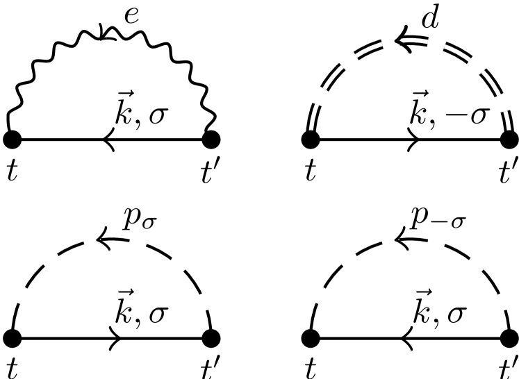
Figure 4: Self-energies in the non-crossing approximation. Wavy, dashed, and double-dashed lines denote, respectively, fully dressed propagators for the empty (e), the single-occupied (p), and the double-occupied (d) configuration. The solid line is the bare Green function for the electrons of the surface. Starting at the left upper corner and proceeding clockwise the diagrams denote, respectively, the self-energies $\Sigma_{0,\sigma}$ $\Sigma_{U,\sigma}$, $\Pi_{d}$, and $\Pi_{e}$ for the Green function $P_{\sigma}$, $D$, and $E$.

The initial conditions for Eqs. (19)–(24) depend on the particular scattering process and how it is modelled. In our case, the initial conditions are

$$\bar{E}^{\rm{R}}(t,t)=\bar{P}_{\sigma}^{\rm{R}}(t,t)=\bar{D}^{\rm{R}}(t,t)=1~{},$$ (28)

and

$$E^{<}(-\infty,-\infty) =n_{e}(-\infty)=0~{},$$ (29)

$$P_{\sigma}^{<}(-\infty,-\infty) =n_{p_{\sigma}}(-\infty)=\delta_{\sigma,1/2}~{},$$ (30)

$$D^{<}(-\infty,-\infty) =n_{d}(-\infty)=0~{}.$$ (31)

Once the equations of motions are solved on a two-dimensional time-grid the instantaneous (pseudo) occurrence probabilities for the ${\rm Sr}^{2+}$, $\rm{Sr}^{+}$, and $\rm{Sr}^{0}$ configuration are simply given by the equal-time Green functions,

$$n_{e}(t) =\bar{E}^{<}(t,t)~{},$$ (32)

$$n_{p_{\sigma}}(t) =\bar{P}^{<}_{\sigma}(t,t)~{},$$ (33)

$$n_{d}(t) =\bar{D}^{<}(t,t)~{}.$$ (34)

Hence, in the notation of pseudo-particles, the neutralization probability

$$\alpha=n_{d}(\infty)~{},$$ (35)

that is, it is the probability of double occupancy after completion of the trajectory.

Nordlander and coworkers Shao et al. (1996, 1994a, 1994b); Langreth and Nordlander (1991) also derived master equations for the occurrence probabilities by approximating the time integrals in the Dyson equations for the Green functions. Depending on the level of sophistication they obtained what they called simple master equations and generalized master equations. In the appendix we state the two sets of master equations arising from Eqs. (19)–(24) by adapting this strategy. The reduction of the set of Dyson equations to a set of master equations utilizes the fact that the functions $\bar{f}_{\varepsilon}^{\gtrless}(t,\bar{t}\,)$ localize the self-energies around the time-diagonal. Thus, provided the Green functions vary not too strongly, they can be put in front of the time integrals. Mathematically, this leads to the constraint, Langreth and Nordlander (1991)

$$R_{0,U}(z)=\Bigg{|}\frac{v\alpha_{0,U}(z)-2\Gamma_{\varepsilon_{0},\varepsilon_{U}}(z)}{\varepsilon_{0,U}(z)-\varepsilon_{F}}\Bigg{|}\ll 1~{},$$ (36)

where $v$ is the projectile velocity. The functions $\alpha_{0,U}(z)$ are defined by requiring $\Gamma_{0,U}(z)=\Delta_{0,U}\exp(-\alpha_{0,U}(z)z)$ which leads to nearly constant values for $\alpha_{0,U}$ verifying thereby the exponential dependence of our level widths. For the upper level the inequality obviously breaks down at the $z=z_{c}$ where it crosses the Fermi energy. As shown by Langreth and Nordlander Langreth and Nordlander (1991) the master equations can still be used at this point if essentially no charge is transferred during the time span the level crosses the Fermi energy. This leads to an additional criterion at $z=z_{c}$. In the next section we will see however that for the upper level of the Sr:Au system investigated by He and Yarmoff He and Yarmoff (2010, 2011) the constraint (36) is violated not only at $z=z_{c}$ but for almost the whole trajectory. Hence, in order to analyze the correlation-driven local-moment physics possibly at work in this experiment the solutions of the full quantum-kinetic equations are needed.

The physical Green functions $G_{\sigma}^{\lessgtr}$ needed for the calculation of the instantaneous spectral densities can be constructed from the standard definition of the less-than and greater-than Green function Kadanoff and Baym (1962) by replacing the original electron operators $c_{\sigma}$ and $c^{\dagger}_{\sigma}$ by pseudo-particle operators according to Eqs. (13)–(14), neglecting vertex corrections, and projecting onto the physical subspace $Q=1$. Thus, $G_{\sigma}^{<}(t,t^{\prime})=\bigl{<}c_{\sigma}^{\dagger}(t^{\prime})c_{\sigma}^{\phantom{{\dagger}}}(t)\bigr{>}$, for instance, becomes

$$G_{\sigma}^{<}(t,t^{\prime}) =\bigl{<}p_{\sigma}^{\dagger}(t^{\prime})e(t^{\prime})e^{\dagger}(t)p_{\sigma}^{\phantom{{\dagger}}}(t)\bigr{>}$$

$$+\bigl{<}d^{\dagger}(t^{\prime})p_{-\sigma}^{\phantom{{\dagger}}}(t^{\prime})p_{-\sigma}^{\dagger}(t)d(t)\bigr{>}~{},$$ (37)

which upon employing $E^{\rm{R}}(t,t^{\prime})=-i\theta(t-t^{\prime})e^{\rm{R}}(t,t^{\prime})$ and $P_{\sigma}^{\rm{R}}(t,t^{\prime})=-i\theta(t-t^{\prime})p_{\sigma}^{\rm{R}}(t,t^{\prime})$ reduces to

$$G_{\sigma}^{<}(t,t^{\prime}) =P_{\sigma}^{<}(t,t^{\prime})\bigl{(}e^{\rm{R}}(t^{\prime},t)+E^{<}(t^{\prime},t)\bigr{)}$$

$$+D^{<}(t,t^{\prime})\bigl{(}p_{-\sigma}^{\rm{R}}(t^{\prime},t)-P_{-\sigma}^{<}(t^{\prime},t)\bigr{)}~{},$$ (38)

where the products $P_{\sigma}^{<}(t,t^{\prime})E^{<}(t^{\prime},t)$ and $D^{<}(t,t^{\prime})P^{<}_{-\sigma}(t^{\prime},t)$ are of order $Q^{2}$ and must thus be projected out to yield

$$G_{\sigma}^{<}(t,t^{\prime})=P_{\sigma}^{<}(t,t^{\prime})e^{\rm{R}}(t^{\prime},t)+D^{<}(t,t^{\prime})p_{-\sigma}^{\rm{R}}(t^{\prime},t)~{}.$$ (39)

A similar calculation leads to

$$G_{\sigma}^{>}(t,t^{\prime})=p_{\sigma}^{\rm{R}}(t,t^{\prime})E^{<}(t^{\prime},t)+d^{\rm{R}}(t,t^{\prime})P_{-\sigma}^{<}(t^{\prime},t)~{},$$ (40)

where $D^{\rm{R}}(t,t^{\prime})=-i\theta(t-t^{\prime})d^{\rm{R}}(t,t^{\prime})$ has been used. Note, in the derivation of the formulae for the physical Green functions we introduced Green functions $e^{\rm R}$, $p^{\rm R}_{\sigma}$, and $d^{\rm R}$, which, in contrast to the Green functions defined in Eq. (17) are retarded Green functions with only the Heaviside function split-off but the phase factor arising from the on-side energies still included.

The spectral densities for removing or adding at time $T$ a physical electron with energy $\omega$ can be obtained from Eq. (39) and Eq. (40) by using difference variables $T=(t+t^{\prime})/2$ and $\tau=t-t^{\prime}$. A Fourier transformation with respect to $\tau=t-t^{\prime}$ yields

$$\rho_{\sigma}^{\lessgtr}(\omega,T)=\dfrac{1}{2\pi}\int_{-\infty}^{\infty}\!\!d\tau\,G_{\sigma}^{\lessgtr}(T+\tau/2,T-\tau/2)\,e^{i\omega\tau}~{}.$$ (41)

The normalization of the spectral densities,

$$\int_{-\infty}^{\infty}\!\!d\omega\,\rho_{\sigma}^{<}(\omega,T) =n_{p_{\sigma}}(T)+n_{d}(T)~{},$$ (42)

$$\int_{-\infty}^{\infty}\!\!d\omega\,\rho_{\sigma}^{>}(\omega,T) =n_{p_{-\sigma}}(T)+n_{e}(T)~{}$$ (43)

is given by the instantaneous occupation of the projectile with a physical electron or a physical hole, respectively, written in terms of the occurrence probabilities introduced above. This follows directly from the equal-time limit of Eqs. (39) and (40) by using $e^{\rm{R}}(t,t)=d^{\rm R}(t,t)=p_{\sigma}^{\rm{R}}(t,t)=1$.

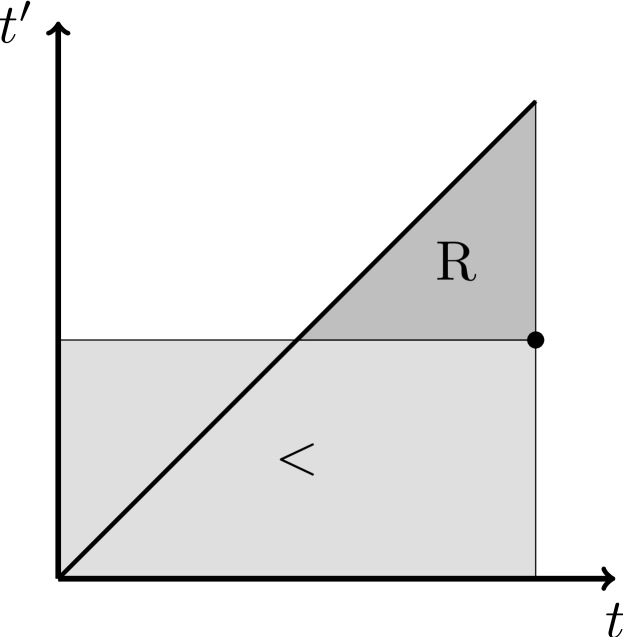
Figure 5: Sketch of the numerical scheme used to solve the double-time equations of motion (19)–(24). The triangle marks the region in the two-dimensional time-grid in which the entries of retarded Green functions have to be known in order to calculate retarded Green functions at the point indicated by the bullet. Likewise, the rectangle marks the region in which the entries of (retarded and less-than) Green functions are required in order to compute less-than Green functions at the point indicated by the bullet.

At the end of this section let us say a few words about the numerics required to solve the two-dimensional integro-differential equations (19)–(24). The discretization strategy proposed by Shao and coworkers Shao et al. (1994a) for $U=\infty$ can be also employed for finite $U$. The main difference is that two more Green functions have to be calculated on the time-grid: $\bar{D}^{\rm R}$ and $\bar{D}^{<}$. The particular structure of the time-integrals leads to the numerical strategy shown in Fig. 5. First, the retarded Green functions are calculated, starting from the time-diagonal where their values are simply set to unity because of the initial condition and then working through the grid points which are on lines parallel to the time-diagonal. To compute retarded Green functions at $(t,t^{\prime})$ only the points in the dark triangle depicted in Fig. 5 have to be sampled. The calculation of the less-than Green functions requires a slightly different scheme. Here the computation first proceeds in the $t$- and then in the $t^{\prime}$-direction, starting from $(-t_{\rm max},-t_{\rm max})$ where the initial condition can be employed and redoing this until one arrives at the desired grid point. Only grid points in the bright rectangular region of Fig. 5 contribute then to the calculation of less-than functions at the point $(t,t^{\prime})$.

The computations are time- and memory-consuming. We employ grid-sizes of up to $3000\times 3000$. Taking advantage of the symmetry of the Green functions, the Green functions in the upper-half of the grid can be obtained from the Green functions of the lower-half by complex conjugation which reduces memory space and number of calculations by one-half. Even then, however, the calculation of one trajectory requires on a $2000\times 2000$ time-grid including the computation of the level widths eight hours of processing time and $400$ Mb memory on a single core. To obtain the temperature dependence of the neutralization probability we let the projectile run through the trajectory for fifty different temperatures. Fortunately, the final charge-state is surprisingly robust against a reduction of the size of the time-grid. Empirically we found the neutralization probability (but not necessarily the occurrence probabilities at intermediate times) to be converged already for a $1000\times 1000$ time-grid. A run for a single temperature requires then only half an hour making an investigation of the temperature dependence of the neutralization process feasible.

IV Results

We now present numerical results. Besides the material parameters listed in Table 1 which should be quite realistic for the Sr:Au system investigated by He and Yarmoff we need the turning point $z_{\rm TP}$ and the velocity $v$ of the strontium projectile. The radius of a strontium atom is around $2.2$ Ångström. It is thus very unlikely for the strontium projectile to come closer to the surface than 4-5 Bohr radii. In atomic units, measuring length in Bohr radii and energy in Hartrees, which we use below if not indicated otherwise, we set therefore $z_{\rm TP}=5$. For the velocity we take the experimentally determined post-collision velocity for the whole trajectory, since it is known that due to loss of memory Onufriev and Marston (1996) the outgoing branch determines the final charge-state of the projectile. In atomic units, $v=0.134$. He and Yarmoff (2010)

Figure 6: The constraints $R_{0}$ and $R_{U}$ as a function of $z$ for the Sr:Au system investigated by He and Yarmoff. He and Yarmoff (2010, 2011) The approximations reducing the double-time quantum kinetics of the Dyson equations to either a set of simple or generalized master equations (see appendix) are valid only for $R_{0,U}\ll 1$. Hence, for $\varepsilon_{0}$ master equations could be used for $z>6$. But for $\varepsilon_{U}$ master equations break down for almost the whole trajectory except for the narrow interval around $z\approx 9$ where the vanishing of the numerator in Eq. (36) leads to small values for $R_{U}$. The peak in $R_{U}$ around $z\approx 12$ signals the point where $\varepsilon_{U}$ crosses the Fermi energy.

First, we investigate if the He-Yarmoff experiment He and Yarmoff (2010, 2011) can be described by the numerically less demanding master equations (either the simple or the generalized set, see appendix). As pointed out in the previous section the master equations should provide a reasonable description of the charge transfer if $R_{0,U}(z)\ll 1$. In Fig. 6 we plot $R_{0,U}(z)$ for $v=0.0134$ and the level widths and energies obtained in Sect. II. While for the second ionization level $\varepsilon_{0}$ master equations could be in fact used all the way down to $z\approx 6$. For the first ionization level $\varepsilon_{U}$ master equations break down not only at the point where the level crosses the Fermi energy but also close to the turning point, where the level width turns out to be too large, and far away from the surface, where the projectile velocity is too high for the master equations to be applicable. Only in a narrow interval around $z\approx 9$, where the high velocity is compensated by the level broadening leading to a small numerator in Eq. (36), $R_{U}$ is small enough to justify master equations also for $\varepsilon_{U}$. Since the two ionization levels are coupled and the charge transfer occurs not only in the narrow range where master equations are applicable to both levels this implies that neither the simple nor the generalized master equations can be used to analyze the Sr:Au system investigated by He and Yarmoff. Instead, the full double-time quantum-kinetics has to be implemented.

Let us now trace–based on the numerical solution of the double-time Dyson equations–for a fixed surface temperature $T_{s}=400$ K important physical quantities while the projectile is on its way through the trajectory. Figure 7 shows in the upper panel the shift and broadening of the ionization levels $\varepsilon_{U}$ and $\varepsilon_{0}$ while the middle panel depicts the instantaneous occurrence probabilities $n_{e}$, $n_{p_{\pm 1/2}}$, and $n_{d}$ for the $\rm{Sr}^{2+}$, $\rm{Sr}^{+}$ and $\rm{Sr}^{0}$ configurations, respectively. The projectile starts at $z=20$ on the left, moves along the incoming branch towards the turning point $z=5$ from which it returns on the outgoing branch again to the distance $z=20$. The strontium projectile starts in the $\rm{Sr}^{+}$ configuration. Thus only the $\varepsilon_{0}$ level is occupied while the $\varepsilon_{U}$ level is empty. During the collision both levels shift upward and broaden. The upper level crosses the Fermi energy at $z=z_{c}\approx 12$. In the course of the collision the occupation probabilities change and the projectile has a certain chance to be at the end in a different charge-state than initially. For the run plotted in Fig. 7 the probability for double occupancy at the end, that is, the probability for neutralization is $\alpha=n_{d}(20)=0.185$. For comparison, we show in the lower panel the instantaneous occupation of $\varepsilon_{U}$ as it is obtained when only this level is kept in the modeling, that is, for a single-level, uncorrelated $U=0$ model. In this case, the neutralization probability $\alpha=0.01$, that is, one order of magnitude smaller.

Figure 7: Instantaneous physical quantities along the trajectory. The strontium projectile starts on the left as an ion at a distance $z=20$ with a velocity $v=0.0134$, reaches the turning point at $z_{\rm TP}=5$ and approaches $z=20$ again thereafter on the right. (a) Energy level diagram. Both levels (solid lines) are broadened according to $\varepsilon\pm\Gamma$ (dashed lines) with the instantaneous $\Gamma$ shown in Fig. 2. (b) Occurrence probabilities at $T_{s}=400$ K for $\mathrm{Sr^{+}}$ (dashed and dot-dashed lines), $\mathrm{Sr^{0}}$ (solid line) and $\mathrm{Sr^{2+}}$ (dotted line) as obtained from the finite$-U$ model. The neutralization probability in this case is $\alpha=n_{d}(20)=0.185$. (c) Occurrence probability of $\mathrm{Sr^{0}}$ as obtained from the uncorrelated $U=0$ model which keeps only the first ionization level, that is, the upper on-site energy $\varepsilon_{U}$. In this case the $\alpha=0.01$. For other surface temperatures $T_{s}$ the results look similar.

The physics behind the results shown in Fig. 7 is as follows. Let us first focus on the first ionization level. Initially, $\varepsilon_{U}$, is below the Fermi energy. Hence, energetically, not the ionic $\rm{Sr}^{+}$ but the neutral $\rm{Sr}^{0}$ configuration is actually favored. However, as can be seen from the vanishing broadening of the level, far away from the surface charge-transfer is negligible. The approaching ion is thus initially stabilized due to lack of coupling. When the coupling becomes stronger for smaller distances $\varepsilon_{U}$ crosses however the Fermi energy. The ion is then energetically stabilized. Roughly speaking, the first ionization level has a chance to capture an electron from the metal only when $|E_{F}-\varepsilon_{U}(t)|<\Gamma_{U}(t)$; in the notation of Sosolik and coworkers the Sr:Au system is in the coupling-dominated regime. Sosolik et al. (2003) From the upper panel in Fig. 7 we see that this is the case only for a very small portion of the trajectory, close to the turning point. As a result, the neutralization probability $\alpha$ should be in any case much smaller than unity as indeed it is. Due to the thermal broadening of the target’s Fermi edge the efficiency of electron-capture into the first ionization level increases with temperature. Thus, if this was the only process involved in the charge-transfer, the neutralization probability should monotonously increase with temperature, contrary to the experimental data which initially increase and then decrease (see below). The charge-transfer must be thus more involved. Indeed, as can be seen in the upper panel in Fig. 7, the second ionization level $\varepsilon_{0}$ comes also close to the Fermi energy. In those parts of the trajectory where $|E_{F}-\varepsilon_{0}(t)|<\Gamma_{0}(t)$ it is thus conceivable that the electron initially occupying $\varepsilon_{0}$ may leave the projectile. That is, holes may transfer from the surface to the second ionization level thereby compensating the electron-transfer into the first. The hole-transfer, absent in the uncorrelated $U=0$ model, tendentiously favors the ion with increasing temperature and should by itself lead to a neutralization probability decreasing with temperature.

That during the collision the ionization levels of strontium come so close to the Fermi energy of the gold target, with the first one crossing it and the second one coming so close to it to enable hole-transfer, led He and Yarmoff to suggest that the neutralization process is driven by electron correlations. The experimentally found negative temperature dependence of $\alpha$ above $T_{s}=600$ K strengthened their conclusion. It agrees qualitatively with what Merino and Marston predicted theoretically on the basis of a correlated-electron model for the neutralization of calcium ions on copper surfaces. Merino and Marston (1998) The work of Shao and coworkers Shao et al. (1996) suggested moreover that the negative temperature dependence of $\alpha$ is caused by a mixed-valence resonance transiently formed in the course of the collision.

Figure 8: Temperature dependence of the neutralization probability $\alpha=n_{d}(20)$ for a $\mathrm{Sr^{+}}$ ion hitting with $v=0.0134$ a gold surface. The turning point $z_{\rm TP}=5$. Also shown are the data of He and Yarmoff. He and Yarmoff (2010) The solid and long-dashed lines are for the finite$-U$ and the uncorrelated $U=0$ model, respectively, showing that correlations enhance the neutralization probability to the experimental order of magnitude. By moving the turning point farther away from the surface we could make the results for $U\neq 0$ to overlap with the experimental data. However, we do not use $z_{\rm TP}$ as a fit parameter for reasons explained in the main text. The non-monotonous temperature dependence of the experimental data cannot be reproduced regardless of the value of the turning point. The dashed-dotted and the dotted line are the neutralization probabilities arising, respectively, from the numerical solution of the set of simple or the set of generalized master equations given in the appendix.

After these qualitative remarks we now discuss the temperature dependence of the neutralization probability quantitatively. In Fig. 8 we show the experimental data of He and Yarmoff He and Yarmoff (2010) and compare it with our theoretical results. For the parameters of Table 1 the theoretical neutralization probability (solid line) turns out a bit too large but it is still of the correct order of magnitude indicating that the material parameters as well as the procedures for calculating the level widths are reasonable. In contrast to the experimental data we find however over the whole temperature range only a weak negative temperature dependence. Also plotted in Fig. 8 is the temperature dependence of the neutralization probability arising from the uncorrelated $U=0$ model (long-dashed line) and–for completeness–the one obtained from the numerical solution of either the set of simple (dashed-dotted line) or the set of generalized master equations (dotted lines) listed at the end of the appendix.

Clearly, without correlations the neutralization probability is too small indicating that correlations play an important role in the charge-transfer from the gold target to the strontium projectile. The chosen turning point $z_{\rm TP}=5$ is in fact most favorable for the uncorrelated model. In reality the turning point may be farther away from the surface. A larger value of $z_{\rm TP}$ leads however to smaller neutralization probabilities. Hence, the results for the uncorrelated model would be pushed farther away from the experimental data while the results for the correlated model would come closer to it. We hesitate however to use $z_{\rm TP}$ as a fit parameter because of the shortcomings of the finite$-U$ non-crossing approximation discussed in the next section.

The neutralization probabilities arising from the master equations are also much smaller than the ones obtained from the full quantum kinetics. Decreasing the turning point would push them of course closer to the experimental data (without reproducing the non-monotonous temperature dependence). However, the numerical values for $R_{0,U}(z)$ shown in Fig. 6 indicate that the approximations leading to the master equations cannot be justified. Hence, the results for $\alpha$ obtained from the master equations should not be artificially pushed towards experimental data by manipulating the turning point. Instead one should–if at all–try to push the correlated $U\neq 0$ data closer to the experimental data by changing the parameters of the Sr:Au system within physically sensible bounds.

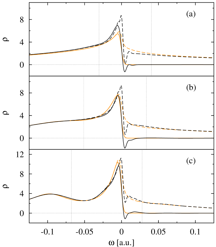
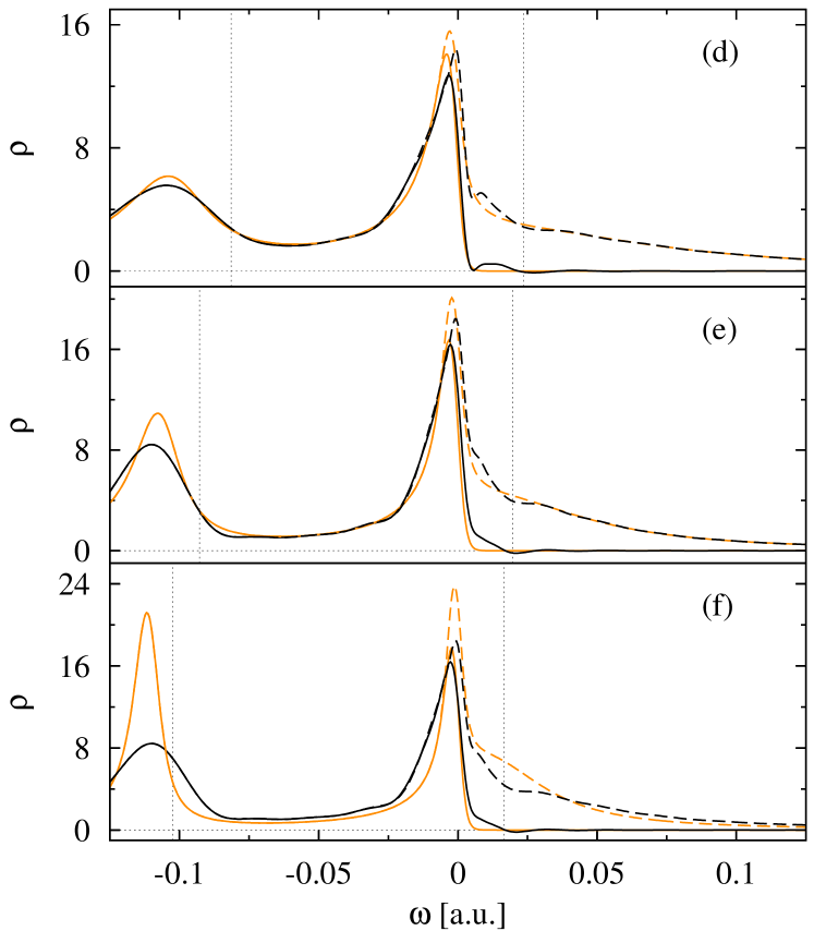
Figure 9: (Color online) Projectile spectral densities summed over the two spin orientations, respectively, at $z=5.0$, $5.5$, $6.0$, $6.5$, $7.0$, and $7.5$ on the outgoing branch of the trajectory [panel (a) to (f)] for a $\mathrm{Sr^{+}}$ ion hitting with $v=0.0134$ a gold surface at temperature $T_{s}=400$ K. For other surface temperatures in the range relevant for the experiment the spectral functions look qualitatively similar. The black lines correspond to the instantaneous spectral densities at the given positions with the solid lines denoting the occupied and the dashed lines the total spectral densities. The vertical dotted lines indicate the instantaneous positions of the on-site energies $\varepsilon_{0}$ and $\varepsilon_{U}$ while the orange lines give the equilibrated occupied (solid lines) and total (dashed lines) spectral densities at the corresponding positions. The target’s Fermi energy is located at $\omega=0$.

Any attempt however to improve the theoretical data by changing the material parameters and hence the single-particle matrix elements of the Anderson-Newns Hamiltonian was unsuccessful. A slight increase of the metal’s work function from $\phi=5.1$ eV to $\phi=5.15$ eV, for instance, decreased the neutralization rate but eliminated at the same time the weak negative temperature dependence. Decreasing the work function from $\phi=5.1$ eV to $\phi=5.05$ eV, on the other hand, increased the theoretical neutralization rate but did also not lead to a stronger negative temperature dependence let alone to a non-monotonous one. Changing the turning point $z_{\rm TP}$ affects the neutralization probability as indicated in the previous paragraph but again wipes out the weak negative temperature dependence. The effect of the Doppler broadening Plihal et al. (1999); Winter (2002); Sosolik et al. (2003) we did not investigate. We take all this as an indication that the correlation effects encoded in the finite-$U$ non-crossing approximation are too fragile. Going beyond this approximation is thus unavoidable.

Another observation should be mentioned. The starting point $z=20$ can be relatively freely chosen. If it is closer to the surface the slopes of the instantaneous occurrence probabilities in Fig. 7 are steeper so that there is hardly any difference in the probabilities at the turning point and no difference at the end of the trajectory. As a result, the final neutralization probability is independent of the precise starting conditions. The loss of memory in charge-transferring atom-surface collisions has been also found by Onufriev and Marston. Onufriev and Marston (1996) It justifies using the pre-collision velocity for the whole trajectory.

In the region where charge-transfer is strongest the two ionization levels overlap. The absence of energy separation together with the conditional temporal weighting due to the dynamics of the collision process makes it very hard to tell a priori whether electron- or hole-transfer dominates the outcome of the collision. Simply changing the matrix elements of the Anderson-Newns model in the hope to reproduce the experimentally found temperature anomaly is pointless as we have indeed seen. Even more so, since the hypothesized electron correlations of the local-moment type strongly distort the projectile’s density of states in the vicinity of the target’s Fermi energy. Any attempt to guess the projectile’s final charge-state on the basis of the single-particle quantities shown in the upper panel of Fig. 7 has thus to fail. In order to see whether the weak negative temperature dependence of $\alpha$ is already a qualitative hint for a mixed-valence scenario to be at work in the neutralization of strontium ions on gold surfaces we calculated therefore the instantaneous spectral densities for the projectile. If local-moment physics is present these functions should feature transient resonances at the target’s Fermi energy.

In Fig. 9 we present for a selected set of distances along the outgoing branch of the trajectory and for $T_{s}=400$ K the instantaneous spectral densities summed over the two spin orientations. The occupied part of the spectral densities (solid black lines), that is, the spectrally resolved probability for removing a physical electron, as well as the total spectral densities (dashed black lines), which in addition contain also the spectrally resolved probability for adding an electron, are shown. For orientation we also plot the equilibrated spectral densities (solid and dashed orange lines) which we obtained by fixing the widths and energetic positions of the levels to the values at that particular distance and then letting the system evolve in time up to the point where it reaches a quasi-stationary state. The negative values of the instantaneous spectral densities close to and at the turning point should not be interpreted too literally. First, we cannot rule out that in the numerical Fourier transformation the Gibbs phenomenon occurs although the results for the equilibrated spectral densities speak against it. Second, and most importantly, the instantaneous spectral densities $\rho_{\sigma}^{\lessgtr}(\omega,T)$ are Wigner distributions in energy $\omega$ and time $T$. These two quantities, however, cannot be measured simultaneously. Usually Wigner distributions deal with quantum-mechanical uncertainties by becoming negative in some regions of the space in which they are defined. Baker Jr. (1958) Integrated over energy, that is, the zeroth-order moments of the Wigner distributions $\rho_{\sigma}^{\lessgtr}(\omega,T)$ give however always the correct occupancies at the particular time as can be easily checked by a comparison with the data obtained from the integration of the equations of motion.

Let us start with panel (a) of Fig. 9 which shows the spectral densities at the closest encounter. The overlapping ionization levels are very broad at this point leading however to a spectral density which due to electronic correlations is enhanced at the Fermi energy $\omega=0$. The uncorrelated model would not give this enhancement. Moving outwards (panels (b)–(f)) the spectral densities change, because of the decreasing widths and the shifting of the ionization levels, developing in addition to the resonance at $\omega=0$ features in the vicinity of the two instantaneous ionization levels which are indicated by the two vertical dotted lines. Although the additional structure due to the upper ionization level is only a high-energy shoulder to the peak at $\omega=0$ the spectral densities develop the shape expected from a quantum impurity: Two charge-transfer peaks and a resonance at the Fermi energy. This can be most clearly seen in panel (f). Since close to the surface the upper charge-transfer peak merges more or less with the peak at the Fermi energy to form a mixed-valence resonance the Sr:Au system is in the mixed-valence regime.

The dominating spectral feature at all the distances shown in Fig. 9 is the enhancement at the target’s Fermi energy. Despite the quantitative discrepancies between the measured and the computed neutralization probabilities our theoretical results for the spectral densities suggest–for realistic single-particle parameters and without any fit parameter–that local-moment physics is present in the Sr:Au system and may thus control the neutralization of ${\rm Sr}^{+}$ on Au surfaces as anticipated by He and Yarmoff. He and Yarmoff (2010) More specifically, from Fig. 7 we read-off that most of the charge-transfer occurs between the turning point $z_{\rm TP}=5$ and the crossing point $z_{c}\approx 12$ whereas from Fig. 9 we see that for these distances the Sr:Au system develops at the Fermi energy of the Au target a mixed-valence resonance with a high-energy tail varying on the scale of the thermal energy. The weak negative temperature dependence we obtain for $\alpha$ is thus due to the mixed-valance resonance in the projectile’s spectral density in accordance with what Merino and Marston predicted for the correlated Ca:Cu system. Merino and Marston (1998) The comparison in Fig. 8 with the results obtained from the uncorrelated $U=0$ model suggests moreover that it is also the mixed-valence resonance which enhances the neutralization probabilities to the experimentally found order of magnitude.

Obviously, our results support He and Yarmoff’s mixed-valence scenario He and Yarmoff (2010, 2011) only qualitatively but not quantitatively. Either the transient local-moment correlations are too weak, occur at the wrong distance, or are simply too short-lived. It requires further theoretical work to tell which one of these possibilities applies.

V Conclusions

We presented a realistically parameterized Anderson-Newns model for charge-transferring collisions between a strontium projectile and a gold target and used the model to analyze from a many-body theoretical point of view the experiment of He and Yarmoff He and Yarmoff (2011, 2010) which indicated that in this type of surface collision a mixed-valence resonance affects the final charge-state of the projectile.

In contrast to the measured neutralization probability which initially increases and then decreases with temperature the computed data show only the correlation-induced enhancement, making the calculated neutralization probability of the correct order of magnitude, and a weak negative temperature dependence. The analysis of the projectile’s instantaneous spectral densities revealed however that both the enhancement and the negative temperature dependence arise from a mixed-valence resonance at the target’s Fermi energy in qualitative agreement with what Merino and Marston found for the Ca:Cu system, Merino and Marston (1998) which is another projectile-target combination which could display local-moment physics. Thus, qualitatively, our results support He and Yarmoff’s interpretation of their data in terms of a mixed-valence resonance.

We followed the theoretical approach of Nordlander and coworkers. Shao et al. (1996, 1994a, 1994b); Langreth and Nordlander (1991) It is based on the non-crossing approximation for Anderson-impurity-type models and contour-ordered Green functions. That we do not find the anomalous temperature dependence of the neutralization probability while having a transient mixed-valence resonance in the instantaneous spectral densities could have two reasons. First, the accuracy of the semi-empirical estimates we developed for the single-particle matrix elements of the Anderson-Newns Hamiltonian may be not enough. The shift of the two ionization levels was obtained from classical considerations based on image charges while the width of the levels was computed from Hartree-Fock and step-potential wave functions. Ab-initio calculations or measurements of these two quantities would be very helpful, in particular, for distances close to the turning point. Second, the finite$-U$ non-crossing approximation most probably does not yield the correct energy scale of the resonance transiently formed at the Fermi energy of the target. Indeed, for finite $U$ the non-crossing approximation does not self-consistently sum-up all leading terms in $1/N$ where $N=2$ is the degeneracy of the 5s level. In equilibrium it is known that the non-crossing approximation underestimates due to this inconsistency the width of the Kondo resonance considerable. Sakai et al. (1988) Systematically summing-up all diagrams to leading order by the one-crossing approximation Otsuki and Kuramoto (2006); Kroha and Wölfle (2005); Pruschke and Grewe (1989); Holm and Schönhammer (1989); Sakai et al. (1988) remedies this shortcoming as does the dynamical $1/N$ approximation used by Merino and Marston Merino and Marston (1998) and equation of motion approaches working directly with the physical Green functions defining the spectral densities. Goldberg et al. (2005) It should be also noted that the temperature anomaly occurs over an interval of only $600$ K corresponding to an energy interval $\Delta E\approx 0.002$ in atomic units. The spectral features in the vicinity of the Fermi energy which drive the anomaly have thus to be known with an energy resolution better than $10^{-3}$.

Specifically our results for the spectral densities make us adhere to the mixed-valence scenario. Besides the above mentioned improvements on the theoretical side further experimental analysis would be however also required to clarify the issue. The velocity dependence of the effect, for instance, would be of great interest because it is the projectile velocity which determines whether the instantaneous correlations get frozen-in and manifest themselves in the final charge-state of the projectile. We would thus expect the experimentally observed temperature anomaly to depend strongly on the projectile’s velocity. Changing the work function and the collision geometry would be also of interest. The former manipulates the point where the upper ionization level crosses the target’s Fermi energy whereas the latter changes the effective temperature via Doppler broadening. The temperature anomaly of the neutralization probability should hence also depend on the work function of the surface and the angle of incident.

It may be easier to realize local-moment physics in electrically biased semiconductor nanostructures but demonstrating it to be also present in charge-transferring atom-surface collisions may open up avenues for further research which are not yet anticipated. The Sr:Au system investigated by He and Yarmoff may well be a very promising candidate.

Appendix

In this appendix we lay out the basic definitions and notations we used in setting up the quantum kinetic equations (19)–(24) of Sec. III. The equations have been originally derived by Shao and coworkers Shao et al. (1994b). As in our previous work on the de-excitation of meta-stable molecules at surfaces, Marbach et al. (2012b) we stay as closely as possible to the notation of Nordlander and coworkers Shao et al. (1994a, b); Langreth and Nordlander (1991) and deviate from it only when it improves the readability of the equations.

Contour-ordered Green functions Kadanoff and Baym (1962); Keldysh (1965) describing the empty, the single occupied, and the double occupied projectile,

$$iE(t,t^{\prime}) =\bigl{\langle}T_{\mathcal{C}}\,e(t)\,e^{\dagger}(t^{\prime})\bigr{\rangle}\;,$$ (44)

$$iP_{\sigma}(t,t^{\prime}) =\bigl{\langle}T_{\mathcal{C}}\,p_{\sigma}^{\phantom{{\dagger}}}(t)\,p_{\sigma}^{\dagger}(t^{\prime})\bigr{\rangle}\;,$$ (45)

$$iD(t,t^{\prime}) =\bigl{\langle}T_{\mathcal{C}}\,d(t)\,d^{\dagger}(t^{\prime})\bigr{\rangle}~{},$$ (46)

as well as metal electrons,

$$iG_{\vec{k},\sigma}(t,t^{\prime})=\bigl{\langle}T_{\mathcal{C}}\,c_{\vec{k},\sigma}^{\phantom{{\dagger}}}(t)\,c_{\vec{k},\sigma}^{\dagger}(t^{\prime})\bigr{\rangle}~{},$$ (47)

where the brackets denote the statistical average with respect to the initial density matrix, constitute the basis of the formalism. The functions $D$ and $E$ are bosonic propagators while $P_{\sigma}$ and $G_{\vec{k},\sigma}$ are fermionic. For any of the four Green functions listed above the analytic pieces, that is, the less-than and the greater-than functions, are given by

$$iH(t,t^{\prime}) =\Theta_{\mathcal{C}}(t-t^{\prime})\,H^{>}(t,t^{\prime})\mp\Theta_{\mathcal{C}}(t^{\prime}-t)\,H^{<}(t,t^{\prime})\;,$$ (48)

where $H$ stands for $E$, $P_{\sigma}$, $D$, or $G_{\vec{k},\sigma}$ and $\Theta_{\mathcal{C}}$ is the Heaviside function defined on the complex time contour. The upper sign holds for fermionic and the lower sign for bosonic Green functions. As usual, the corresponding retarded functions read

$$iH^{R}(t,t^{\prime})=\theta(t-t^{\prime})\bigl{[}H^{>}(t,t^{\prime})\pm H^{<}(t,t^{\prime})\bigr{]}~{},$$ (49)

where again the upper (lower) sign holds for fermionic (bosonic) functions and $\theta$ is now the Heaviside function on the real time axis.

Similarly, the self-energies $\Sigma_{\sigma}$, $\Pi_{\rm e}$, and $\Pi_{\rm d}$ for the single occupied, the empty, and the double occupied projectile can be split into analytic pieces which in turn give rise to retarded self-energies,

$$i\Sigma_{\sigma}^{\rm R}(t,t^{\prime})=\theta(t-t^{\prime})\bigl{[}\Sigma_{\sigma}^{>}(t,t^{\prime})+\Sigma_{\sigma}^{<}(t,t^{\prime})\bigr{]}~{},$$ (50)

$$i\Pi_{\rm e,d}^{\rm R}(t,t^{\prime})=\theta(t-t^{\prime})\bigl{[}\Pi_{\rm e,d}^{>}(t,t^{\prime})-\Pi_{\rm e,d}^{<}(t,t^{\prime})\bigr{]}~{}.$$ (51)

Within the non-crossing approximation the metal electrons are undressed. Hence, below $G_{\vec{k},\sigma}$ is always the bare propagator and no self-energy has to be specified for the metal electrons. Shao et al. (1996, 1994a, 1994b); Langreth and Nordlander (1991)

On the real-time axis the analytic pieces of the Green function obey the set of Dyson equations ($\hbar=1$):

$$i\frac{\partial}{\partial t}E^{\rm{R}}(t,t^{\prime}) =\delta(t-t^{\prime})+\int_{-\infty}^{\infty}\!\!d\bar{t}\,\Pi^{\rm R}_{\rm e}(t,\bar{t}\,)E^{\rm{R}}(\bar{t},t^{\prime})~{}$$ (52)

$$\Bigl{[}i\frac{\partial}{\partial t}-\varepsilon_{0}(t)\Bigl{]}P^{\rm{R}}_{\sigma}(t,t^{\prime}) =\delta(t-t^{\prime})+\int_{-\infty}^{\infty}\!\!d\bar{t}\,\Sigma_{\sigma}^{\rm R}(t,\bar{t}\,)P_{\sigma}^{\rm{R}}(\bar{t},t^{\prime})~{}$$ (53)

$$\Bigl{[}i\frac{\partial}{\partial t}-\varepsilon_{0}(t)-\varepsilon_{U}(t)\Bigl{]}D^{\rm{R}}(t,t^{\prime}) =\delta(t-t^{\prime})+\int_{-\infty}^{\infty}\!\!d\bar{t}\,\Pi_{\rm d}^{\rm R}(\bar{t},t)D^{\rm{R}}(\bar{t},t^{\prime})$$ (54)

$$i\frac{\partial}{\partial t}E^{<}(t,t^{\prime}) =\int^{\infty}_{-\infty}\!\!d\bar{t}\,\Pi_{\rm e}^{\rm R}(t,\bar{t}\,)E^{<}(\bar{t},t^{\prime})+\int^{\infty}_{-\infty}d\bar{t}\,\Pi_{\rm e}^{<}(t,\bar{t}\,)E^{\rm A}(\bar{t},t^{\prime})$$ (55)

$$\Bigl{[}i\frac{\partial}{\partial t}-\varepsilon_{0}(t)\Bigl{]}P_{\sigma}^{<}(t,t^{\prime}) =\int^{\infty}_{-\infty}\!\!d\bar{t}\,\Sigma_{\sigma}^{\rm R}(t,\bar{t}\,)P_{\sigma}^{<}(\bar{t},t^{\prime})+\int^{\infty}_{-\infty}d\bar{t}\,\Sigma_{\sigma}^{<}(t,\bar{t}\,)P_{\sigma}^{\rm A}(\bar{t},t^{\prime})$$ (56)

$$\Bigl{[}i\frac{\partial}{\partial t}-\varepsilon_{0}(t)-\varepsilon_{U}(t)\Bigl{]}D^{<}(t,t^{\prime}) =\int^{\infty}_{-\infty}\!\!d\bar{t}\,\Pi_{\rm d}^{\rm R}(t,\bar{t}\,)D^{<}(\bar{t},t^{\prime})+\int^{\infty}_{-\infty}d\bar{t}\,\Pi_{\rm d}^{<}(t,\bar{t}\,)D^{\rm A}(\bar{t},t^{\prime})~{}.$$ (57)

The self-energies in the non-crossing approximation are shown in Fig. 4, where the self-energy $\Sigma_{\sigma}$ for the single occupied projectile is split into two pieces, $\Sigma_{\sigma,0}$ and $\Sigma_{\sigma,U}$, depending on whether the empty or the double occupied state appears as a virtual state. Applying standard diagrammatic rules Lifshitz and Pitaevskii (1981) together with the Langreth-Wilkins rules Langreth and Wilkins (1972) given in our notation in Ref. Marbach et al. (2012b) yields after projection to the $Q=1$ subspace Langreth and Nordlander (1991); Wingreen and Meir (1994); Aguado and Langreth (2003) the following mathematical expressions for the analytic pieces of the self-energies:

$$\Pi^{\gtrless}_{\rm d}(t,t^{\prime}) =\sum_{\sigma}\int\frac{d\varepsilon}{2\pi}K_{\varepsilon}^{\gtrless}(t,t^{\prime})P_{-\sigma}^{\gtrless}(t,t^{\prime})~{},$$ (58)

$$\Pi^{\rm R}_{\rm d}(t,t^{\prime}) =\sum_{\sigma}\int\frac{d\varepsilon}{2\pi}K_{\varepsilon}^{>}(t,t^{\prime})P_{-\sigma}^{\rm R}(t,t^{\prime})~{},$$ (59)

$$\Pi^{\gtrless}_{\rm e}(t,t^{\prime}) =\sum_{\sigma}\int\frac{d\varepsilon}{2\pi}K_{\varepsilon}^{\lessgtr}(t^{\prime},t)P_{\sigma}^{\gtrless}(t,t^{\prime})~{},$$ (60)

$$\Pi^{\rm R}_{\rm e}(t,t^{\prime}) =\sum_{\sigma}\int\frac{d\varepsilon}{2\pi}K_{\varepsilon}^{<}(t^{\prime},t)P_{\sigma}^{\rm R}(t,t^{\prime})~{},$$ (61)

$$\Sigma^{\gtrless}_{\sigma,0}(t,t^{\prime}) =\int\frac{d\varepsilon}{2\pi}K_{\varepsilon}^{\gtrless}(t,t^{\prime})E^{\gtrless}(t,t^{\prime})~{},$$ (62)

$$\Sigma^{\rm R}_{\sigma,0}(t,t^{\prime}) =\int\frac{d\varepsilon}{2\pi}K_{\varepsilon}^{>}(t,t^{\prime})E^{\rm R}(t,t^{\prime})~{},$$ (63)

$$\Sigma^{\gtrless}_{\sigma,U}(t,t^{\prime}) =\int\frac{d\varepsilon}{2\pi}K_{\varepsilon}^{\lessgtr}(t^{\prime},t)D^{\gtrless}(t,t^{\prime})~{}$$ (64)

$$\Sigma^{\rm R}_{\sigma,U}(t,t^{\prime}) =\int\frac{d\varepsilon}{2\pi}K_{\varepsilon}^{<}(t^{\prime},t)D^{\rm R}(t,t^{\prime})~{}$$ (65)

with

$$K_{\varepsilon}^{\gtrless}(t,t^{\prime})=\sqrt{\Gamma_{\varepsilon}(t)\Gamma_{\varepsilon}(t^{\prime})}f^{\gtrless}(\varepsilon)e^{-i\varepsilon(t-t^{\prime})}~{},$$ (66)

where $\varepsilon$ is an energy variable to be integrated over.

In obtaining the self-energies we took advantage of the fact that the propagator of the metal electrons is undressed and spin independent. As a result, $\Sigma_{\sigma,0}$ and $\Sigma_{\sigma,U}$ (and thus $\Sigma_{\sigma}$) are independent of the electron spin. Furthermore, we assumed the tunneling matrix element $V_{\vec{k}}(t)$ to factorize in the variables $t$ and $\vec{k}$. In our case this is approximately true since the strongest time dependence in Eq. (9) comes from the modified Bessel function $K_{\alpha}$ giving rise to a nearly exponential time dependence of $V_{\vec{k}}(t)$. The function

$$\Gamma_{\varepsilon}(t,t^{\prime}) =2\pi\sum_{\vec{k}}V_{\vec{k}}(t)V^{*}_{\vec{k}}(t^{\prime})\delta(\varepsilon-\varepsilon_{\vec{k}})$$ (67)

initially appearing in the self-energies can thus be approximately rewritten as Shao et al. (1994a); Langreth and Nordlander (1991)

$$\Gamma_{\varepsilon}(t,t^{\prime})\simeq\sqrt{\Gamma_{\varepsilon}(t)\Gamma_{\varepsilon}(t^{\prime})}$$ (68)

with $\Gamma_{\varepsilon}(t)$ defined by Eq. (11) leading eventually to the expressions for the self-energies given above.

Inserting the self-energies (58)–(65) into the Dyson equations (52)–(57) and rewriting the equations in terms of the reduced Green functions defined by Eqs. (17) and (18) yields after an approximate $\varepsilon$-integration Eqs. (19)–(24) of Sec. III.

Due to the approximate $\varepsilon$-integration the functions $\bar{K}_{\varepsilon}^{\gtrless}(t,t^{\prime})$ enter the formalism. In the definition (25) of these functions the subscript $\varepsilon$ denotes not an energy variable but the functional dependence on $\varepsilon(t)$. To see this consider the Dyson equation (52). In terms of reduced Green functions it reads

$$\partial_{t}\bar{E}^{\rm R}(t,t^{\prime}) =-\sum_{\sigma}\int_{t^{\prime}}^{t}d\bar{t}\int\frac{d\varepsilon}{2\pi}\sqrt{\Gamma_{\varepsilon}(t)\Gamma_{\varepsilon}(\bar{t}\,)}f^{<}(\varepsilon)\exp\left[-i\!\int_{\bar{t}}^{t}\!\!d\tau\,(\varepsilon_{0}(\tau)-\varepsilon)\right]\bar{P}_{\sigma}^{\rm R}(t,\bar{t}\,)\bar{E}^{\rm R}(\bar{t},t^{\prime})$$ (69)

$$\simeq-\sum_{\sigma}\int_{t^{\prime}}^{t}d\bar{t}\sqrt{\Gamma_{\varepsilon_{0}(t)}(t)\Gamma_{\varepsilon_{0}(\bar{t}\,)}(\bar{t}\,)}f^{<}(\bar{t}-t)\exp\left[-i\!\int_{\bar{t}}^{t}\!\!d\tau\,\varepsilon_{0}(\tau)\right]\bar{P}_{\sigma}^{\rm R}(t,\bar{t}\,)\bar{E}^{\rm R}(\bar{t},t^{\prime})$$ (70)

$$=-\sum_{\sigma}\int_{t^{\prime}}^{t}d\bar{t}\sqrt{\Gamma_{\varepsilon_{0}(t)}(t)\Gamma_{\varepsilon_{0}(\bar{t}\,)}(\bar{t}\,)}\bar{f}_{\varepsilon_{0}}^{<}(\bar{t},t)\bar{P}_{\sigma}^{\rm R}(t,\bar{t}\,)\bar{E}^{\rm R}(\bar{t},t^{\prime})$$ (71)

$$=-\sum_{\sigma}\int_{t^{\prime}}^{t}d\bar{t}\bar{K}_{\varepsilon_{0}}^{<}(\bar{t},t)\bar{P}_{\sigma}^{\rm R}(t,\bar{t}\,)\bar{E}^{\rm R}(\bar{t},t^{\prime})$$ (72)

with $\bar{K}_{\varepsilon_{0}}^{<}(\bar{t},t)$ as defined in Eq. (25). The step from the first to the second line involves the approximate $\varepsilon$-integration resulting in the Fourier transformation of the Fermi function and in fixing the energy variables of the level widths as indicated. We did not attempt to derive it mathematically by an asymptotic stationary-phase analysis. Bleistein and Handelsman (1986) Instead we followed Shao and coworkers Shao et al. (1994b) and adopted a qualitative, physics-based reasoning. It yields the very intuitive equation (70) and reduces moreover the numerical effort considerably because it is no longer necessary to perform at each time-grit point $(t,t^{\prime})$ an $\varepsilon$-integration. Alternatively $\Gamma_{\varepsilon}(t)$ could be replaced in (69) by an average over the energy range of the conduction band and then put in front of the $\varepsilon$-integral. Shao et al. (1994a) But this seems to be even more ad-hoc.

Similar manipulations can be performed for the other Dyson equations. At the end one obtains equations (19)–(24) of Sec. III. The equations are identical to the ones given by Shao and coworkers in the book edited by Rabalais Shao et al. (1994b) if–as we did–the pseudo-particle operator $p_{\sigma}$ is taken to be fermionic.

The kinetic equations (19)–(24) are a complicated set of two-dimensional integro-differential equations. Nordlander and coworkers Shao et al. (1994a, b); Langreth and Nordlander (1991) showed however that in situations where the functions $\bar{f}_{\varepsilon}^{\gtrless}(t,\bar{t}\,)$ and hence the self-energies are sufficiently peaked at $t=\bar{t}$ the Dyson equations for the less-than Green functions can be reduced to master equations for the occurrence probabilities which are numerically less expensive. Depending on whether retarded Green functions are taken at equal times and hence pushed in front of the time integrals or not two sets of master equations can be derived: the simple and the generalized master equations. Shao et al. (1994a, b); Langreth and Nordlander (1991) Applying this reasoning to Eqs. (19)–(24) yields at the level where retarded Green functions are taken at equal times a set of simple master equations,

$$\dfrac{d}{dt}n_{e}(t)= -2\Gamma_{0}(t)f^{<}\bigl{(}\varepsilon_{0}(t)\bigr{)}n_{e}(t)+\Gamma_{0}(t)f^{>}\bigl{(}\varepsilon_{0}(t)\bigr{)}\Bigl{(}n_{p_{1/2}}(t)+n_{p_{-1/2}}(t)\Bigr{)}~{},$$ (73)

$$\dfrac{d}{dt}n_{p_{\sigma}}(t)= -\Bigl{(}\Gamma_{0}(t)f^{>}\bigl{(}\varepsilon_{0}(t)\bigr{)}+\Gamma_{U}(t)f^{<}\bigl{(}\varepsilon_{U}(t)\bigr{)}\Bigr{)}n_{p_{\sigma}}(t)$$

$$+\Gamma_{0}(t)f^{<}\bigl{(}\varepsilon_{0}(t)\bigr{)}n_{e}(t)+\Gamma_{U}(t)f^{>}\bigl{(}\varepsilon_{U}(t)\bigr{)}n_{d}(t)~{},$$ (74)

$$\dfrac{d}{dt}n_{d}(t)= -2\Gamma_{U}(t)f^{>}\bigl{(}\varepsilon_{U}(t)\bigr{)}n_{d}(t)+\Gamma_{U}(t)f^{<}\bigl{(}\varepsilon_{U}(t)\bigr{)}\Bigl{(}n_{p_{1/2}}(t)+n_{p_{-1/2}}(t)\Bigr{)}~{},$$ (75)

and at the advanced level, where retarded Green functions are kept non-diagonal in time, a set of generalized master equations,

$$\dfrac{d}{dt}n_{e}(t)= -2n_{e}(t)\sum_{\sigma}\int_{-\infty}^{t}\!\!d\bar{t}\,\operatorname{Im}\Bigl{(}\bar{K}_{\varepsilon_{0}}^{<}(\bar{t},t)\bar{P}_{\sigma}^{\rm{R}}(t,\bar{t}\,)\Bigr{)}+2\sum_{\sigma}n_{p_{\sigma}}(t)\int_{-\infty}^{t}\!\!d\bar{t}\,\operatorname{Im}\Bigl{(}\bar{K}_{\varepsilon_{0}}^{>}(\bar{t},t)\left[\bar{E}^{\rm{R}}(t,\bar{t}\,)\right]^{*}\Bigr{)}~{},$$ (76)

$$\dfrac{d}{dt}n_{p_{\sigma}}(t)= -2n_{p_{\sigma}}(t)\int_{-\infty}^{t}\!\!d\bar{t}\,\operatorname{Im}\Bigl{(}\bar{K}_{\varepsilon_{0}}^{>}(t,\bar{t}\,)\bar{E}^{\rm{R}}(t,\bar{t}\,)+\bar{K}_{\varepsilon_{U}}^{<}(\bar{t},t)\bar{D}^{\rm{R}}(t,\bar{t}\,)\Bigr{)}$$

$$+2n_{e}(t)\int_{-\infty}^{t}\!\!d\bar{t}\,\operatorname{Im}\Bigl{(}\bar{K}_{\varepsilon_{0}}^{<}(t,\bar{t}\,)\left[\bar{P}_{\sigma}^{\rm{R}}(t,\bar{t}\,)\right]^{*}\Bigr{)}+2n_{d}(t)\int_{-\infty}^{t}\!\!d\bar{t}\,\operatorname{Im}\Bigl{(}\bar{K}_{\varepsilon_{U}}^{>}(\bar{t},t)\left[\bar{P}_{\sigma}^{\rm{R}}(t,\bar{t}\,)\right]^{*}\Bigr{)}~{},$$ (77)

$$\dfrac{d}{dt}n_{d}(t)= -2n_{d}(t)\sum_{\sigma}\int_{-\infty}^{t}\!\!d\bar{t}\,\operatorname{Im}\Bigl{(}\bar{K}_{\varepsilon_{U}}^{>}(t,\bar{t}\,)\bar{P}_{\sigma}^{\rm{R}}(t,\bar{t}\,)\Bigr{)}+2\sum_{\sigma}n_{p_{\sigma}}(t)\int_{-\infty}^{t}\!\!d\bar{t}\,\operatorname{Im}\Bigl{(}\bar{K}_{\varepsilon_{U}}^{<}(t,\bar{t}\,)\left[\bar{D}^{\rm{R}}(t,\bar{t}\,)\right]^{*}\Bigr{)}~{}$$ (78)

with occurrence probabilities $n_{e}(t)$, $n_{p_{\sigma}}(t)$, and $n_{d}(t)$ as defined in Eqs. (32)–(34). The retarded Green functions required in the generalized master equations can be obtained by utilizing the localization of $\bar{f}_{\varepsilon}^{\gtrless}(t,\bar{t}\,)$ around the time-diagonal also in the Dyson equations for the retarded Green functions. As a result one obtains,

$$\bar{E}^{\rm{R}}(t,t^{\prime}) =\exp\left[-\sum_{\sigma}\int_{t^{\prime}}^{t}\!\!d\tau\int_{t^{\prime}}^{\tau}\!\!d\bar{t}\,\bar{K}_{\varepsilon_{0}}^{<}(\bar{t},\tau)\bar{P}_{\sigma}^{\rm{R}}(\tau,\bar{t}\,)\right]~{},$$ (79)

$$\bar{P}^{\rm{R}}_{\sigma}(t,t^{\prime}) =\exp\left[-\int_{t^{\prime}}^{t}\!\!d\tau\int_{t^{\prime}}^{\tau}\!\!d\bar{t}\,\Bigl{(}\bar{K}_{\varepsilon_{0}}^{>}(\tau,\bar{t}\,)\bar{E}^{\rm{R}}(\tau,\bar{t}\,)+\bar{K}_{\varepsilon_{U}}^{<}(\bar{t},\tau)\bar{D}^{\rm{R}}(\tau,\bar{t}\,)\Bigr{)}\right]~{},$$ (80)

$$\bar{D}^{\rm{R}}(t,t^{\prime}) =\exp\left[-\sum_{\sigma}\int_{t^{\prime}}^{t}\!\!d\tau\int_{t^{\prime}}^{\tau}\!\!d\bar{t}\,\bar{K}_{\varepsilon_{U}}^{>}(\tau,\bar{t}\,)\bar{P}_{-\sigma}^{\rm{R}}(\tau,\bar{t}\,)\right]~{}.$$ (81)

A rigorous determination of the range of validity of these equations by asymptotic techniques Bleistein and Handelsman (1986) is complicated because the functions $\bar{f}_{\varepsilon}^{\gtrless}(t,\bar{t}\,)$ are not only localized around the time-diagonal but also strongly oscillating. Simple saddle-point arguments are thus not sufficient but have to be augmented by a stationary-phase analysis. Analyzing moreover the whole set of Dyson equations by these techniques seems to be impractical. Langreth and Nordlander Langreth and Nordlander (1991) investigated therefore the validity of the approximations empirically and developed qualitative criteria which have to be satisfied for master equations to provide a reasonable description of the charge-transfer between the projectile and the target surface. As shown in Sect. IV the basic constraint (36) they developed is not satisfied for the Sr:Au system investigated by He and Yarmoff. He and Yarmoff (2010, 2011) The full double-time quantum kinetic equations have thus to be solved to analyze this experiment.

References

- Monreal (2014) R. C. Monreal, Progr. Surf. Sci. 89, 80 (2014).
- Winter and Burgdörfer (2007) H.-P. Winter and J. Burgdörfer, eds., Slow heavy-particle induced electron emission from solid surface (Springer-Verlag, Berlin Heidelberg, 2007).
- Winter (2002) H. Winter, Phys. Rep. 367, 387 (2002).
- Rabalais (1994) J. W. Rabalais, ed., Low energy ion-surface interaction (Wiley and Sons, New York, 1994).
- Los and Geerlings (1990) J. Los and J. J. C. Geerlings, Phys. Rep. 190, 133 (1990).
- Brako and Newns (1989) R. Brako and D. M. Newns, Rep. Prog. Phys. 52, 655 (1989).
- Modinos (1987) A. Modinos, Progr. Surf. Sci. 26, 19 (1987).
- Yoshimori and Makoshi (1986) A. Yoshimori and K. Makoshi, Prog. Surf. Sci. 21, 251 (1986).
- Newns et al. (1983) D. M. Newns, K. Makoshi, R. Brako, and J. N. M. van Wunnik, Physica Scripta T6, 5 (1983).
- Kraus et al. (2007) W. Kraus, H.-D. Falter, U. Fantz, P. Franzen, B. Heinemann, P. McNeely, R. Riedl, and E. SPeth, Rev. Sci. Instrum. 79, 02C108 (2007).
- Lieberman and Lichtenberg (2005) M. A. Lieberman and A. J. Lichtenberg, Principles of plasma discharges and materials processing (Wiley-Interscience, New York, 2005).
- Rabalais (2003) J. W. Rabalais, Principles and applications of ion scattering spectrometry: Surface chemical and structural analysis (Wiley and Sons, New York, 2003).
- Harada et al. (1997) Y. Harada, S. Masuda, and H. Ozaki, Chem. Rev. 97, 1897 (1997).
- Hewson (1993) A. C. Hewson, The Kondo problem to heavy fermions (Cambridge University Press, Cambridge, 1993).
- Fulde (1995) P. Fulde, Electron correlations in molecules and solids (Springer Verlag, Berlin, 1995).
- Chang and Chen (2009) A. M. Chang and J. C. Chen, Rep. Prog. Phys. 72, 096501 (2009).
- Pustilnik and Glazman (2004) M. Pustilnik and L. Glazman, J. Phys. Condens. Matter 16, R513 (2004).
- Aguado and Langreth (2003) R. Aguado and D. C. Langreth, Phys. Rev. B 67, 245307 (2003).
- Goldhaber-Gordon et al. (1998a) D. Goldhaber-Gordon, H. Shtrikman, D. Mahalu, D. Abusch-Magder, U. Meirav, and M. A. Kastner, Nature 391, 156 (1998a).
- Cronenwett et al. (1998) S. M. Cronenwett, T. H. Oosterkamp, and L. P. Kouwenhoven, Science 281, 540 (1998).
- Goldhaber-Gordon et al. (1998b) D. Goldhaber-Gordon, J. Gores, M. A. Kastner, H. Shtrikman, D. Mahalu, and U. Meirav, Phys. Rev. Lett. 81, 5225 (1998b).
- Wingreen and Meir (1994) N. S. Wingreen and Y. Meir, Phys. Rev. B 49, 11040 (1994).
- Grabert and Devoret (1992) H. Grabert and M. H. Devoret, eds., Single charge tunneling: Coulomb blockade phenomena in nanostructures (Plenum Press, New York, 1992).
- Nghiem and Costi (2014) H. T. M. Nghiem and T. A. Costi, Phys. Rev. B 90, 035129 (2014).
- Lechtenberg and Anders (2014) B. Lechtenberg and F. B. Anders, Phys. Rev. B 90, 045117 (2014).
- Mühlbacher et al. (2011) L. Mühlbacher, D. F. Urban, and A. Komnik, Phys. Rev. B 83, 075107 (2011).
- Cohen and Rabani (2011) G. Cohen and E. Rabani, Phys. Rev. B 84, 075150 (2011).
- Shao et al. (1996) H. Shao, P. Nordlander, and D. C. Langreth, Phys. Rev. Lett. 77, 948 (1996).
- Merino and Marston (1998) J. Merino and J. B. Marston, Phys. Rev. B 58, 6982 (1998).
- He and Yarmoff (2011) X. He and J. A. Yarmoff, Nucl. Instrum. Meth. Phys. Res. B 269, 1195 (2011).
- He and Yarmoff (2010) X. He and J. A. Yarmoff, Phys. Rev. Lett. 105, 176806 (2010).
- Shao et al. (1994a) H. Shao, D. C. Langreth, and P. Nordlander, Phys. Rev. B 49, 13929 (1994a).
- Shao et al. (1994b) H. Shao, D. C. Langreth, and P. Nordlander, in Low energy ion-surface interaction, edited by J. W. Rabalais (Wiley and Sons, New York, 1994b), p. 117.
- Langreth and Nordlander (1991) D. C. Langreth and P. Nordlander, Phys. Rev. B 43, 2541 (1991).
- Kasai and Okiji (1987) H. Kasai and A. Okiji, Surface science 183, 147 (1987).
- Nakanishi et al. (1988) H. Nakanishi, H. Kasai, and A. Okiji, Surface science 197, 515 (1988).
- Romero et al. (2009) M. A. Romero, F. Flores, and E. C. Goldberg, Phys. Rev. B 80, 235427 (2009).
- Bajales et al. (2007) N. Bajales, J. Ferrón, and E. C. Goldberg, Phys. Rev. B 76, 245431 (2007).
- Goldberg et al. (2005) E. C. Goldberg, F. Flores, and R. C. Monreal, Phys. Rev. B 71, 035112 (2005).
- Onufriev and Marston (1996) A. V. Onufriev and J. B. Marston, Phys. Rev. B 53, 13340 (1996).
- Marston et al. (1993) J. B. Marston, D. R. Andersson, E. R. Behringer, B. H. Cooper, C. A. DiRubio, G. A. Kimmel, and C. Richardson, Phys. Rev. B 48, 7809 (1993).
- Clementi and Roetti (1974) E. Clementi and C. Roetti, Atomic. Data Nucl. Data Tables 14, 177 (1974).
- Gadzuk (1967a) J. W. Gadzuk, Surface Science 6, 133 (1967a).
- Gadzuk (1967b) J. W. Gadzuk, Surface Science 6, 159 (1967b).
- Gadzuk (2009) J. W. Gadzuk, Phys. Rev. B 79, 073411 (2009).
- Coleman (1984) P. Coleman, Phys. Rev. B 29, 3035 (1984).
- Kotliar and Ruckenstein (1986) G. Kotliar and A. E. Ruckenstein, Phys. Rev. Lett. 57, 1362 (1986).
- Kadanoff and Baym (1962) L. P. Kadanoff and G. Baym, Quantum Statistical Mechanics (Benjamin, New York, 1962).
- Keldysh (1965) L. V. Keldysh, Sov. Phys. JETP 20, 1018 (1965).
- Otsuki and Kuramoto (2006) J. Otsuki and Y. Kuramoto, J. Phys. Soc. Jpn. 75, 064707 (2006).
- Kroha and Wölfle (2005) J. Kroha and P. Wölfle, J. Phys. Soc. Jpn. 74, 16 (2005).
- Pruschke and Grewe (1989) T. Pruschke and N. Grewe, Z. Phys. B 74, 439 (1989).
- Holm and Schönhammer (1989) J. Holm and K. Schönhammer, Solid State Commun. 69, 969 (1989).
- Sakai et al. (1988) O. Sakai, M. Motizuki, and T. Kasuya, in Core level spectroscopy in condensed systems, edited by J. Kanamori and A. Kotani (Springer Verlag, Berlin, 1988), p. 45.
- Nordlander and Tully (1988) P. Nordlander and J. C. Tully, Phys. Rev. Lett. 61, 990 (1988).
- Nordlander and Tully (1990) P. Nordlander and J. C. Tully, Phys. Rev. B 42, 5564 (1990).
- Borisov and Wille (1995) A. G. Borisov and U. Wille, Surface science 338, L875 (1995).
- More et al. (1998) W. More, J. Merino, R. Monreal, P. Pou, and F. Flores, Phys. Rev. B 58, 7385 (1998).
- Valdés et al. (2005) D. Valdés, E. C. Goldberg, J. M. Blanco, and R. C. Monreal, Phys. Rev. B 71, 245417 (2005).
- Marbach et al. (2012a) J. Marbach, F. X. Bronold, and H. Fehske, Eur. Phys. J. D 66, 106 (2012a).
- Marbach et al. (2012b) J. Marbach, F. X. Bronold, and H. Fehske, Phys. Rev. B 86, 115417 (2012b).
- Marbach et al. (2011) J. Marbach, F. X. Bronold, and H. Fehske, Phys. Rev. B 84, 085443 (2011).
- Kürpick and Thumm (1996) P. Kürpick and U. Thumm, Phys. Rev. A 54, 1487 (1996).
- Slater (1930) J. C. Slater, Phys. Rev. 36, 57 (1930).
- Abramowitz and Stegun (1973) M. Abramowitz and I. A. Stegun, eds., Handbook of mathematical functions (Dover Publications, Inc., New York, 1973).
- Langreth and Wilkins (1972) D. C. Langreth and J. W. Wilkins, Phys. Rev. B 6, 3189 (1972).
- Sosolik et al. (2003) C. E. Sosolik, J. R. Hampton, A. C. Lavery, B. H. Cooper, and J. B. Marston, Phys. Rev. Lett. 90, 013201 (2003).
- Plihal et al. (1999) M. Plihal, D. C. Langreth, and P. Nordlander, Phys. Rev. B 59, 13322 (1999).
- Baker Jr. (1958) G. A. Baker Jr., Phys. Rev. 109, 2198 (1958).
- Lifshitz and Pitaevskii (1981) E. M. Lifshitz and L. P. Pitaevskii, Physical Kinetics (Pergamon Press, New York, 1981).
- Bleistein and Handelsman (1986) N. Bleistein and R. A. Handelsman, Asymptotic expansion of integrals (Dover publications, New York, 1986).