Pseudospin, velocity and Berry phase in a bilayer graphene

Abstract

Hamiltonian and eigenstate problem is formulated for a bilayer graphene in terms of Clifford’s geometric algebra Cl_3,1 and respective multivectors. It is shown that such approach allows to perform analytical calculations in a simple way if geometrical algebra rotors are used. The measured quantities are express through spectrum and rotation half-angle of the pseudospin that appears in geometric algebra rotors. Properties of free charge carriers – pseudospin, velocity and Berry phase – in a bilayer graphene are investigated in the presence of the external voltage applied between the two layers.

1 Introduction

Bilayer graphene (BLG) consists of two graphene monolayers A and B that are typically aligned in the Bernal stacking arrangement. The study of BLG has started in 2006 after the appearance of E. McCann’s and V. I. Fal’ko’s paper [1]. A unique feature of the BLG is its tunable energy band structure by external voltage applied between A and B layers. The opening of the gap in exfoliated bottom-gated BLG was demonstrated experimentally by A. B. Kuzmenko et al [2]. A comprehensive description of BLG properties and respective references can be found in review articles [3, 4] and monograph [5].

The geometric algebra (GA), or more precisely a family of algebras Cl_p,q, where $p$ and $q$ define the metric of space, can be used as an alternative mathematical instrument in classical, quantum and relativistic physics [6, 7, 8]. The main advantage of GA is that it is coordinate or representation free, and unifies all parts of applied mathematics (vector calculus, matrix algebra, dyadics, tensor algebra, differential forms etc) in a single coherent entity. Classical and quantum problems can be formulated in the same space without any need to resort to abstract Hilbert space. The GA has a very powerful tool called the “rotor” which is related with quantum mechanical spinors and, therefore, with the Schrödinger and Dirac equations in multidimensional spaces with variable metric [9]. Recently, the GA and rotors were applied to analyze quantum ring [10], monolayer graphene and quantum well [11, 12, 13, 14]. Since calculations in GA are performed in a coordinate free way, the GA is structurally compact and allows geometric interpretation of formulas. This is very appealing as compared to abstract Hilbert space approach. In this paper we apply relativistic Cl_3,1 algebra and its rotors to analyze bilayer graphene properties. In the next section we calculate the rotors and in subsequent sections the rotors are used to analyze the pseudospin (Sec. 3), velocity (Sec. 4) and Berry phase (Sec. 5). In the Appendix, a summary of GA operations and formulae used in this paper is presented.

2 BLG in geometric algebra formulation

The BLG consists of two stacked carbon monolayers that will be numbered $1$ and $2$. The elementary cell of each monolayer has two inequivalent sites $A$ and $B$, therefore, the wave function in the tight binding approximation at least has four components which will be arranged in the order $\{\psi_{A1},\psi_{A2},\psi_{B1},\psi_{B2}\}$. In this Hilbert space basis the considered BLG Hamiltonian is

$$\hat{H}=\eta\left[\begin{array}[]{cccc}U&0&\gamma_{0}k_{-}&0\\ 0&-U&\eta\gamma_{1}&\gamma_{0}k_{-}\\ \gamma_{0}k_{+}&\eta\gamma_{1}&U&0\\ 0&\gamma_{0}k_{+}&0&-U\end{array}\right]$$ (1)

where $k_{\pm}=k_{x}\pm\mathrm{i}k_{y}$ with $k_{x}$ and $k_{y}$ being the components of wave vector in the graphene plane. The constant $\gamma_{0}=-\langle\psi_{A1}|\hat{H}|\psi_{B1}\rangle=-\langle\psi_{A2}|\hat{H}|\psi_{B2}\rangle$ is the intralayer hopping energy and $\gamma_{1}=\langle\psi_{A2}|\hat{H}|\psi_{B1}\rangle$ is the interlayer nearest neighbor hopping energy. The energy $2U$ is the potential difference between the layers, also called the asymmetry term. $\eta=+1$ for $K$-valley and $\eta=-1$ for $K^{\prime}$-valley. The intrinsic electron spin in the Hamiltonian (1) is not included. In the following all energies will be normalized to intralayer hopping energy $\gamma_{0}$. The wave vector and its components will be normalized by $k_{c}=2\pi/a$, where $a$ is the graphene lattice constant. It is assumed that $\hbar=1$.

a) b)

Figure 1: The spectrum of bilayer graphene, Eq. (2), a) in absence, $U=0$ and b) in presence, $U=0.1$, of the interlayer voltage $2U$. $\gamma_{1}=0.1$.

The dependence of normalized to $\gamma_{0}$ dispersion energies of the Hamiltonian (1) on the wave vector magnitude $k=(k_{x}^{2}+k_{y}^{2})^{1/2}$ is

$$E^{(i)}=\pm\sqrt{k^{2}+U^{2}+\frac{\gamma_{1}^{2}}{2}\pm\frac{1}{2}\sqrt{\gamma_{1}^{4}+4k^{2}(4U^{2}+\gamma_{1}^{2})}}\,,$$ (2)

where $i$ is the band number as indicated in Fig. 1. The spectrum (2) is the same for both $K$ and $K^{\prime}$ valleys. When $U=0$ the energy gap is absent, Fig. 1a, and the spectrum reduces to $E_{0}^{(i)}=\pm(\gamma_{1}/2)\pm\sqrt{k^{2}+(\gamma_{1}/2)^{2}}$. If the potential difference $2U$ is created between the layers the energy gap opens and parabolic-like spectrum of two bands transforms to “Mexican-hat” spectrum as shown in Fig. 1b. This brings about altogether new physical properties in BLG. Here and in all subsequent figures the interlayer coupling energy is assumed to be $\gamma_{1}=0.1$ which is close to experimental values: $\gamma_{1}/\gamma_{0}=0.3\text{[eV]}/2.9\text{[eV]}\approx 0.1$ and $\gamma_{1}/\gamma_{0}=0.4\text{[eV]}/3.0\text{[eV]}\approx 0.13$ [3].

Using matrix representation of Cl_3,1 algebra the Hamiltonian (1) can be decomposed into sum of matrices

$$\hat{H}=\eta(k_{x}\hat{e}_{1}+k_{y}\hat{e}_{2})-\frac{\gamma_{1}}{2}\Big{(}\mathrm{i}\,\hat{e}_{3}\hat{e}_{1}+\hat{I}\hat{e}_{2}\Big{)}+\eta U\hat{I}\hat{e}_{3},$$ (3)

where for $4\times 4$ matrices denoted by hats are given in the Appendix 7.1. It should be stressed that the matrix representation of GA elements is not unique and, it is important, in principle is not needed in solving the problem at all. It is presented for a convenience to help the reader to connect the present geometric algebra approach [see Eq. (4) below] with the standard Hilbert space Hamiltonian (1).

Using the replacement rules from the Appendix 7.2, the matrix BLG Hamiltonian (3) can be mapped to GA Hamiltonian function of spinor $\psi$,

$$H(\psi)=\eta\mathbf{k}\psi I\!\mathbf{e}_{3}-\frac{\gamma_{1}}{2}\mathbf{e}_{2}\Big{(}\psi+\mathbf{e}_{4}\psi\mathbf{e}_{4}\Big{)}\mathbf{e}_{3}+\eta U\mathbf{e}_{3}\psi\mathbf{e}_{3},$$ (4)

where $\mathbf{k}=k_{x}\mathbf{e}_{1}+k_{y}\mathbf{e}_{2}$ is the in-plane wave vector in terms of basis vectors $\mathbf{e}_{i}$ of Cl_3,1 algebra. The spinor $\psi$ that appears in this Hamiltonian function consists of even grade blades only (see Eq. (46) in the Appendix 7.2). In the Clifford space Hamiltonian (4), the basis coordinate vector $\mathbf{e}_{3}$ is directed along pseudospin quantization axis, Fig. 2.

Now the eigenmultivector equation in GA

$$H(\psi^{(i)})=E^{(i)}\psi^{(i)}$$ (5)

is solved using the Hamiltonian (4), where $E^{(i)}$ is the eigenenergy ($i$-th energy band) and $\psi^{(i)}$ is the respective eigenmultivector, by the method proposed in [12, 13]. The method is based on the fact that the eigenvalue equation (5) can be transformed to rotor equation of the form $R\mathbf{e}_{3}R^{-1}=\mathbf{a}$, where the rotor $R$ brings the unit vector $\mathbf{e}_{3}$parallel to the quasispin quantization axis to a final position $\mathbf{a}$ determined by the Hamiltonian (4). The spectrum follows from the condition that the rotation preserves the length of a rotated vector. The respective eigenmultivectors then can be constructed from bivectors that represent rotation planes which are made up of the quantization axis and final direction determined by the eigenvalue, Fig. 2.

To transform the Eq. (5) to rotors, at first, the multivector is divided into two parts $\psi=\psi_{+}+\psi_{-}$, where $\psi_{+}$ is invariant to spatial inversion, $\overline{\psi}_{+}=\psi_{+}$, and $\psi_{-}$ changes its sign to opposite, $\overline{\psi}_{-}=-\psi_{-}$ (see the Appendix 7.3). Then the multivector eigenequation $H(\psi)=E\psi$, where the band index was temporally suppressed, can be decomposed into pair of coupled multivector equations,

$$\begin{split}E\psi_{+}&=\eta\mathbf{k}\psi_{-}I\!\mathbf{e}_{3}+\eta U\mathbf{e}_{3}\psi_{+}\mathbf{e}_{3},\\ E\psi_{-}&=\eta\mathbf{k}\psi_{+}I\!\mathbf{e}_{3}+\eta U\mathbf{e}_{3}\psi_{-}\mathbf{e}_{3}-\gamma_{1}\mathbf{e}_{2}\psi_{-}\mathbf{e}_{3}.\end{split}$$ (6)

The method of solution of (6) relies on the fact that $\psi_{+}$ and $I\psi_{-}$, where $I$ is the pseudoscalar of Cl_3,1 algebra, are the rotors in 3D Euclidean space. For this purpose one expresses $\psi_{-}$ from the first equation of (6), and inserts into the second equation. After some algebraic manipulations and remembering that GA is a noncommutative algebra one can construct the following linear equation for $\psi_{+}$,

$$R\psi_{+}\mathbf{e}_{3}=L\psi_{+},$$ (7)

where

$$\begin{split}R=&E[2\eta UI\!\mathbf{e}_{3}-k^{-2}\gamma_{1}\mathbf{e}_{1}(k_{x}+k_{y}\mathbf{e}_{12})^{2}\mathbf{e}_{34}],\\ L=&(E^{2}+U^{2}-k^{2})I+k^{-2}\eta U\gamma_{1}\mathbf{e}_{1}(k_{x}+k_{y}\mathbf{e}_{12})^{2}\mathbf{e}_{4}.\end{split}$$

The Eq. (7) can be rewritten in a form of rotor equation

$$\psi_{+}\mathbf{e}_{3}\tilde{\psi}_{+}=LR^{-1}\equiv\mathbf{a},$$ (8)

where $\psi_{+}$ represents the rotor in 3D space and the tilde denotes the reversion operation. The vector $\mathbf{a}$ simplifies to

$$\begin{split}\mathbf{a}&=\frac{\gamma_{1}\xi}{Ek^{2}}\,\mathbf{k}\mathbf{e}_{2}\mathbf{k}+\frac{\eta U(2\xi+1)}{E}\,\mathbf{e}_{3},\\ \xi&=\frac{E^{2}-k^{2}-U^{2}}{4U^{2}+\gamma_{1}^{2}}.\end{split}$$ (9)

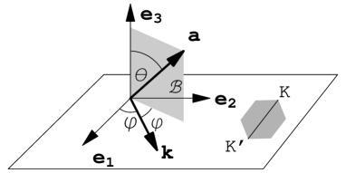
Figure 2: Basis vectors $\mathbf{e}_{1}$, $\mathbf{e}_{2}$ and $\mathbf{e}_{3}$, the wave vector $\mathbf{k}$, and the rotation plane $\hat{\mathcal{B}}=\mathbf{e}_{3}\!\wedge\!\hat{\mathbf{a}}$ that contains $\mathbf{e}_{3}$ and vector $\mathbf{a}$. The vector $\mathbf{e}_{3}$ is perpendicular to graphene plane (square). The line that connects $K$ and $K^{\prime}$ valleys in the Brillouin zone is parallel to $\mathbf{e}_{1}$.

The geometric product $\mathbf{k}\mathbf{e}_{2}\mathbf{k}$ in polar coordinates simplifies to $\mathbf{k}\mathbf{e}_{2}\mathbf{k}/k^{2}=\sin(2\varphi)\,\mathbf{e}_{1}-\cos(2\varphi)\,\mathbf{e}_{2}$, where $\varphi$ is the angle between $\mathbf{e}_{1}$ and $\mathbf{k}$. Figure 2 shows geometric interpretation of equation (8). The initial vector $\mathbf{e}_{3}$, which is perpendicular to graphene plane and coincides with quasispin quantization axis, is brought to the final vector $\mathbf{a}=\psi_{+}\mathbf{e}_{3}\tilde{\psi}_{+}$ with the half-angle rotor $\psi_{+}$, where $\psi_{+}^{-1}=\tilde{\psi}_{+}$ (see Appendix 7.3). One can distinguish two extreme cases. When the interlayer interaction is switched off, i. e. when $\gamma_{1}=0$, then $\mathbf{a}\|\mathbf{e}_{3}$ and the rotations can be performed only around $\mathbf{e}_{3}$ axis. In opposite case, when $U=0$, the final vector $\mathbf{a}$ lies in the graphene plane, so that the rotation angle in this case is $\theta=\pi/2$, Fig. 2. In general case, $\theta$ is determined by competition between the interlayer interaction strength $\gamma_{1}$ and external voltage $2U$ between the layers.

For $\psi_{+}$ to be a rotor it should be normalized, $\psi_{+}\tilde{\psi}_{+}=1$. This guarantees that $\psi_{+}$ brings $\mathbf{e}_{3}$ to a unit vector $\hat{\mathbf{a}}=\mathbf{a}/|\mathbf{a}|$. Mathematically the requirement that length remains constant is expressed by condition $\hat{\mathbf{a}}^{2}=1$, or in a full form

$$\hat{\mathbf{a}}^{2}=\frac{(E^{2}-k^{2}+U^{2})^{2}+U^{2}\gamma_{1}^{2}}{E^{2}(4U^{2}+\gamma_{1}^{2})}=1.$$ (10)

If this fourth order polynomial equation is solved with respect to energy $E$ we shall get the spectrum (2) of the bilayer graphene. From this we conclude that all possible vectors $\hat{\mathbf{a}}^{(i)}$ in the rotor equation

$$\psi_{+}^{(i)}\mathbf{e}_{3}\tilde{\psi}_{+}^{(i)}=\hat{\mathbf{a}}^{(i)}$$ (11)

are related with the dispersion $E^{(i)}$ of the $i$-th band and thus the vectors $\hat{\mathbf{a}}^{(i)}$ represent the points on a unit sphere.

The knowledge of $\hat{\mathbf{a}}^{(i)}=\mathbf{a}^{(i)}/|\mathbf{a}^{(i)}|$ and condition (10) allow to construct the rotor for the $i$-th energy band,

$$\psi^{(i)}_{+}=\mathrm{e}^{\mathcal{B}^{(i)}\theta^{(i)}/2}=\cos\frac{\theta^{(i)}}{2}+\mathcal{B}^{(i)}\sin\frac{\theta^{(i)}}{2}.$$ (12)

Here $\mathcal{B}^{(i)}=\mathbf{e}_{3}\wedge\hat{\mathbf{a}}^{(i)}$ is the bivector that determines the unit oriented plane where the rotation takes plane by angle $\theta^{(i)}$, Fig. 2. The cosine of the angle $\theta^{(i)}$ between $\mathbf{e}_{3}$ and $\hat{\mathbf{a}}^{(i)}$ can be found from the inner GA product $\cos\theta^{(i)}=\mathbf{e}_{3}\cdot\hat{\mathbf{a}}^{(i)}$,

$$\begin{split}&c^{(i)}\equiv\cos\theta^{(i)}=\\ &\eta\frac{U(2E^{(i)2}-2k^{2}+2U^{2}+\gamma_{1}^{2})}{\sqrt{4U^{2}+\gamma_{1}^{2}}\,\sqrt{(E^{(i)2}-k^{2}+U^{2})^{2}+U^{2}\gamma_{1}^{2}}}\,.\end{split}$$ (13)

Elementary algebraic calculations allow to rearrange the rotor-spinor (12) to the following form

$$\psi_{+}^{(i)}=\frac{1}{\sqrt{2}}\Big{(}\sqrt{1+c^{(i)}}+(1-c^{(i)})\frac{\mathbf{e}_{3}\mathbf{k}\mathbf{e}_{2}\mathbf{k}}{k^{2}}\Big{)},$$ (14)

which in the expanded form consists of scalar and two bivectors, $\mathbf{e}_{23}$ and $\mathbf{e}_{31}$, i. e. it consists of even blades only.

The knowledge of $\psi_{+}^{(i)}$ allows to find the second spinor-rotor $(I\psi_{-}^{(i)})$. It can be expressed through $\psi_{+}$ if the first equation of the system (6) is used,

$$(I\psi_{-}^{(i)})=\frac{\mathbf{k}}{k^{2}}\Big{(}\eta E^{(i)}\psi_{+}^{(i)}\mathbf{e}_{3}-U\mathbf{e}_{3}\psi_{+}^{(i)}\Big{)},$$ (15)

which can be rearranged to the following form

$$\begin{split}\psi_{-}^{(i)}=&\frac{\sqrt{1+c^{(i)}}}{\sqrt{2}\,k}\Big{(}U-E^{(i)}\eta\Big{)}\mathrm{e}^{-\mathbf{e}_{12}\,\varphi}\mathbf{e}_{24}+\\ &\frac{\sqrt{1-c^{(i)}}}{\sqrt{2}\,k}\Big{(}U+E^{(i)}\eta\Big{)}\mathrm{e}^{\mathbf{e}_{12}\,\varphi}\mathbf{e}_{34}.\end{split}$$ (16)

The total eigenmultivector $\psi^{(i)}$ is a sum (14) and (16),

$$\psi^{(i)}=\psi_{+}^{(i)}+\psi_{-}^{(i)}.$$ (17)

It satisfies the eigenequation (5). In calculating the physical averages the eigenmultivector $\psi^{(i)}$ must be normalized. The square of the normalization constant is

$$N^{(i)2}=(E^{(i)2}+k^{2}+U^{2}-2\eta Uc^{(i)}E^{(i)})/k^{2}.$$ (18)

In conclusion, the eigenmultivectors have been expressed through band energies $E^{(i)}$ and cosines $c^{(i)}=\cos\theta^{(i)}$ of the rotation angle $\theta$ shown in Fig. 2. The following sign rules should be applied to the eigenmultivectors of individual bands:

$$\psi^{(i)}=\begin{cases}&\psi^{(1)}\quad\text{and }E^{(i)}\rightarrow-E^{(1)},\\ &\psi^{(2)}\quad\text{and }E^{(i)}\rightarrow-E^{(2)},\text{ and }c^{(i)}\rightarrow-c^{(2)},\\ &\psi^{(3)}\quad\text{and }\ c^{(i)}\rightarrow-c^{(3)},\\ &\psi^{(4)}\quad\text{Eq.}~{}\eqref{psipm},\\ \end{cases}$$ (19)

where $c^{(i)}$ is given by Eq. (13). We shall remind that the superscripts $(2)$, $(4)$ label the conduction bands and $(1)$, $(3)$ label the valence bands. Below the eigenmultivectors (19) will be used to analyze pseudospin, velocity and Berry’s phase properties.

3 Pseudospin

In Hilbert basis $\{\psi_{A1},\psi_{A2},\psi_{B1},\psi_{B2}\}$ the pseudospin components are described by matrices

$$\hat{P}_{x}=\left[\begin{array}[]{cc}0&\hat{1}\\ \hat{1}&0\end{array}\right],\ \hat{P}_{y}=\mathrm{i}\left[\begin{array}[]{cc}0&-\hat{1}\\ \hat{1}&0\end{array}\right],\ \hat{P}_{z}=\left[\begin{array}[]{cc}\hat{1}&0\\ 0&-\hat{1}\end{array}\right].$$ (20)

In Cl_3,1 they should be replaced by following GA functions (see Appendix 7.2)

$$\begin{split}P_{1}(\psi)&=\mathbf{e}_{1}\psi I\!\mathbf{e}_{3},\\ P_{2}(\psi)&=\mathbf{e}_{2}\psi I\!\mathbf{e}_{3},\\ P_{3}(\psi)&=\mathbf{e}_{3}\overline{\psi}\mathbf{e}_{3}=\mathbf{e}_{34}\psi\mathbf{e}_{34}.\\ \end{split}$$ (21)

These function satisfy commutation relations of type $P_{1}\big{(}P_{2}(\psi)\big{)}-P_{2}\big{(}P_{1}(\psi)\big{)}=2IP_{3}(\psi)\mathbf{e}_{34}$ etc. From all of this follows that the average Cartesian components of the pseudospin are

$$\begin{split}\langle P_{1}\rangle&=\langle\psi^{\dagger}\mathbf{e}_{1}\psi I\!\mathbf{e}_{3}\rangle,\\ \langle P_{2}\rangle&=\langle\psi^{\dagger}\mathbf{e}_{2}\psi I\!\mathbf{e}_{3}\rangle,\\ \langle P_{3}\rangle&=\langle\psi^{\dagger}\mathbf{e}_{34}\psi\mathbf{e}_{34}\rangle,\end{split}$$ (22)

and the average pseudospin and its squared module are

$$\begin{split}\mathcal{P}&=\langle P_{1}\rangle\mathbf{e}_{23}+\langle P_{2}\rangle\mathbf{e}_{31}+\langle P_{3}\rangle\mathbf{e}_{12},\\ |\mathcal{P}|^{2}&=\mathcal{P}\tilde{\mathcal{P}}=\langle P_{1}\rangle^{2}+\langle P_{2}\rangle^{2}+\langle P_{3}\rangle^{2}.\end{split}$$ (23)

Note that in GA the pseudospin is the bivector (oriented plane) rather than vector (oriented line), because in GA the rotations in an oriented plane can be generalized to multidimensional spaces in contrast to rotations around axis [6]. Formula (23) decomposes the pseudospin into three components (mutually perpendicular planes). Calculations give that, in accordance with a symmetry of the problem, the pseudospin of the $i$-th band can be expressed as

$$\mathcal{P}^{(i)}=p_{\|}^{(i)}(\cos\varphi\,\mathbf{e}_{23}+\sin\varphi\,\mathbf{e}_{31})+p_{\bot}^{(i)}\mathbf{e}_{12},$$ (24)

where $\varphi$ is the angle between $\mathbf{e}_{1}$ and $\mathbf{k}$, Fig. 2. In terms of the standard vectorial calculus we would say that the first term in (24) with the amplitude $p_{\|}^{(i)}$ corresponds to dual vector $\mathbf{P}_{\|}$ that lies in the graphene plane and is parallel to the wave vector, $\mathbf{P}_{\|}\|\mathbf{k}$, while the second term with $p_{\bot}^{(i)}$component represents the dual vector $\mathbf{P}_{\bot}$ which is perpendicular to plane. In GA terms this is expressed as $\mathbf{P}=\mathbf{P}_{\|}+\mathbf{P}_{\bot}=\mathcal{P}I_{3}^{-1}$, where $I_{3}=\mathbf{e}_{1}\!\wedge\!\mathbf{e}_{2}\!\wedge\!\mathbf{e}_{3}$ is 3D subspace pseudoscalar.

After insertion of $\psi^{(i)}=\psi_{+}^{(i)}+\psi_{-}^{(i)}$ into (22) one finds that for the “Mexican-hat”-type conduction (4) and valence (1) bands the amplitudes are

$$\begin{split}p_{\|}^{(1,4)}&=\frac{2k\big{(}\mp\eta E^{(1,4)}-r^{(1,4)}U\big{)}}{E^{(1,4)2}+k^{2}+U^{2}\pm 2\eta r^{(1,4)}E^{(1,4)}U}\,,\\ p_{\bot}^{(1,4)}&=\frac{r^{(1,4)}(-E^{(1,4)2}+k^{2}-U^{2})\mp 2\eta E^{(1,4)}U}{E^{(1,4)2}+k^{2}+U^{2}\pm 2\eta r^{(1,4)}E^{(1,4)}U},\end{split}$$ (25)

where upper/lower sign is for band (1)/(4). The amplitudes for parabolic-like conduction (2) and valence (3) bands are

$$\begin{split}p_{\|}^{(2,3)}&=\frac{2k\big{(}\mp\eta E^{(2,3)}+r^{(2,3)}U\big{)}}{E^{(2,3)2}+k^{2}+U^{2}\mp 2\eta r^{(2,3)}E^{(2,3)}U}\,,\\ p_{\bot}^{(2,3)}&=\frac{r^{(2,3)}(E^{(2,3)2}-k^{2}+U^{2})\mp 2\eta E^{(2,3)}U}{E^{(2,3)2}+k^{2}+U^{2}\mp 2\eta r^{(2,3)}E^{(2,3)}U},\end{split}$$ (26)

where upper/lower sign is for band (2)/(3). Since $\eta=1$ for $K$-valley and $\eta=-1$ for $K^{\prime}$-valley, and the cosine functions $r^{(i)}$ is proportional to $\eta$ [see Eq. (13)] it follows that the pseudospins of $K$ and $K^{\prime}$ valleys are proportional to $\eta$, in other words the pseudospins in $K$ and $K^{\prime}$ valleys have opposite signs (directions).

a) b)

Figure 3: Pseudospin components parallel $p_{\|}$ and perpendicular $p_{\bot}$ to graphene surface as a function of the wave vector at three voltages: $1-U=0.001$, $2-U=0.1$, $3-U=0.2$. a) $p_{\|}^{(1,4)}$, and $p_{\bot}^{(1,4)}$ correspond to Mexican-hat shaped bands $(1)$ and $(4)$. b) $p_{\|}^{(2,3)}$ and $p_{\bot}^{(2,3)}$ correspond to parabolic-like bands $(2)$ and $(3)$. In all cases $\gamma_{1}=0.1$.

Figure 3 shows the amplitudes $p_{\|}^{(i)}$ and $p_{\bot}^{(i)}$ calculated with (25) and (26) as a function of wave vector $\mathbf{k}$ magnitude. It is seen that at large wave vectors, when electron kinetic energy predominates over interlayer coupling energy $\gamma_{1}$ and voltage $U$, the pseudospin vector $\mathbf{P}$ lies in the graphene plane in all cases, i. e. $\mathbf{P}_{\bot}\approx 0$. Then $\mathbf{P}\approx\mathbf{P}_{\|}$ and $\mathbf{P}$ is either parallel [bands (1) and (4)] or antiparallel [bands (2) and (3)] to $\mathbf{k}$. At small $\mathbf{k}$ values, or when either $\gamma_{1}$ or applied voltage $2U$ begins to predominate, the component $p_{\bot}^{(i)}$ perpendicular to graphene plane may be large. At $U=0$ the parallel component is

$$p_{\|}^{(i)}=\pm\frac{2\eta E_{0}^{(i)}k}{E_{0}^{(i)2}+k^{2}},$$ (27)

where plus sign is for bands (3,4) and minus sign is for bands (1,2), and $E_{0}^{(i)}\equiv E^{(i)}(U=0)$. If $k\rightarrow 0$ then $p_{\|}^{(i)}\rightarrow 0$.

Figure 3b shows that for parabolic-like bands when $U\rightarrow 0$ we have $p_{\bot}^{(2,3)}=0$ (note that curve 1 coincides with the horizontal axis), and the pseudospin vector totally lies in the graphene plane and is either parallel (in $K$-valley) or antiparallel (in $K^{\prime}$-valley) to $\mathbf{k}$ for all wave vectors (energies). Since $E_{0}^{(i)}=\pm(\gamma_{1}/2)\pm\sqrt{k^{2}+(\gamma_{1}/2)^{2}}$ when $U=0$, the point $\mathbf{k}=0$ appears to be singular for bands having “Mexican-hat” shape. Therefore, it is convenient to introduce a tilt angle $\vartheta$, which is defined as the angle between pseudospin vector $\mathbf{P}$ and graphene plane. The tangent of the tilt angle then is $\tan\vartheta=p_{\bot}/p_{\|}$.

a) b)

Figure 4: The tilt angle $\vartheta$ of the pseudospin vector as a function of the normalized wave vector $k$ for the conduction, CB(2) and CB(4), and valence, VB(1) and VB(3), bands at different interlayer voltages: $2U=0.05;\ 0.2;\ 0.4$. $\gamma_{1}=0.1$.

Figure 4 shows the dependence of $\vartheta$ on the wave vector magnitude when the external voltage between the layers is $2U=0.05;0.2;0.4$. At high wave vector values the angle $\vartheta$ goes to zero, i. e., as mentioned, the pseudospin vector lies in the graphene plane. The steps in the Fig. 4b are related with extremal points in the “Mexican-hat” energy dispersion, Fig. 1b. At $U=0$ and $k=0$ the step overlaps with the ordinate axis.

4 Charge carrier velocity

The velocity in quantum mechanics is determined by vectorial operator $\hat{\mathbf{v}}=\partial\hat{H}/\partial\mathbf{k}$. The velocity components for Hamiltonian (1) are

$$\hat{v}_{x}=\eta\left[\begin{array}[]{cc}0&\hat{1}\\ \hat{1}&0\end{array}\right],\quad\hat{v}_{y}=\mathrm{i}\eta\left[\begin{array}[]{cc}0&-\hat{1}\\ \hat{1}&0\end{array}\right].$$ (28)

After mapping to GA with the replacement rules from Appendix 7.2 we find the corresponding formulas

$$\hat{v}_{x}|\psi\rangle\,\longrightarrow\,\eta\mathbf{e}_{1}\psi I\!\mathbf{e}_{3},\quad\hat{v}_{y}|\psi\rangle\,\longrightarrow\,\eta\mathbf{e}_{2}\psi I\!\mathbf{e}_{3}.$$ (29)

These components consist of even grade GA elements. GA expressions (29) can also be obtained directly by taking partial derivatives of GA Hamiltonian (4) with respect to wave vector components:

$$\begin{split}v_{x}(\psi)&=\frac{\partial H(\psi)}{\partial k_{x}}=\eta\mathbf{e}_{1}\psi I\!\mathbf{e}_{3},\\ v_{y}(\psi)&=\frac{\partial H(\psi)}{\partial k_{y}}=\eta\mathbf{e}_{2}\psi I\!\mathbf{e}_{3}.\end{split}$$ (30)

The average electron velocity then is

$$\langle\mathbf{v}\rangle=\langle\psi^{\dagger}v_{x}(\psi)\rangle\mathbf{e}_{1}+\langle\psi^{\dagger}v_{y}(\psi)\rangle\mathbf{e}_{2}.$$ (31)

By convention, in GA the angular brackets on the right-hand side indicate that the scalar part should be taken. The velocity can also be defined in a coordinate free way if the following vector differential operator that acts in graphene plane is introduced

$$\nabla_{\mathbf{k}}=\mathbf{e}_{1}\frac{\partial}{\partial k_{x}}+\mathbf{e}_{2}\frac{\partial}{\partial k_{y}}.$$ (32)

Then the average electron velocity can be written in the following coordinate-free form

$$\langle\mathbf{v}\rangle=\dot{\nabla}_{\mathbf{k}}\langle\psi^{\dagger}\dot{H}(\psi)\rangle,$$ (33)

where the dagger operation is defined by formula (52) in the Appendix 7.3. Since $\mathbf{e}_{i}\psi\neq\psi\mathbf{e}_{i}$, the operator $\nabla_{\mathbf{k}}$ cannot be pushed through spinor $\psi^{\dagger}$. The pair of the overdots in (33) indicates that only the partial derivatives $\partial/\partial k_{x}$ and $\partial/\partial k_{y}$ act on the Hamiltonian directly.

Figure 5: Average electron velocity vs wave vector in conduction bands of BLG. $v_{F}$ is the asymptotic velocity when $k\rightarrow\infty$. $U=0.1$.

Calculations with (31) or (33) give the following general expression for the $i$-th band average velocity

$$\begin{split}&\langle\mathbf{v}^{(i)}\rangle=v^{(i)}\big{(}\mathbf{e}_{1}\cos\varphi+\mathbf{e}_{2}\sin\varphi\big{)},\\ &v^{(i)}=\pm\frac{2k(\pm E^{(i)}+\eta r^{(i)}U)}{E^{(i)2}+k^{2}+U^{2}\pm 2\eta E^{(i)}r^{(i)}U},\\ \end{split}$$ (34)

where the sign in the amplitude $v^{(i)}$ depends on band index. It is seen that $\langle\mathbf{v}^{(i)}\rangle\|\mathbf{k}$, in accordance with the isotropic character of energy bands. If the velocity (34) is expanded in a full form the dependence on valley index $\eta$ vanishes. This means that in both $K$ and $K^{\prime}$ valleys the electron velocity magnitude and direction are the same. Figure 5 illustrates the average velocity of electron in the conduction band calculated with (34), where the change of sign in $v^{(4)}$ is related with the “Mexican-hat” character of the conduction band dispersion. The same velocities are found for valence bands.

It can be shown that the average velocity can be obtained in a simpler way, directly from the respective band,

$$\langle\mathbf{v}^{(i)}\rangle=\nabla_{\mathbf{k}}E^{(i)}=\frac{\partial E^{(i)}}{\partial k_{x}}\mathbf{e}_{1}+\frac{\partial E^{(i)}}{\partial k_{y}}\mathbf{e}_{2},$$ (35)

where $\nabla_{\mathbf{k}}$ is the vectorial derivative (32).

5 Berry phase

At low free carrier energies the Berry phase of BLG is equal to $2\pi$ [1]. As we shall see, in the presence of the interlayer potential the Berry phase no longer remains a multiple of $\pi$.

The Berry phase $\Gamma$ can be defined through a sum of matrix elements between adjacent points [15]

$$\Gamma=-\mathrm{i}\lim_{N\rightarrow\infty}\sum_{j=0}^{N-1}\log\langle\psi_{j}|\psi_{j+1}\rangle,$$ (36)

where $j$ is the state index. The sum in (36) is closed so that the initial and final states coincide, $|\psi_{0}\rangle=|\psi_{N}\rangle$. If the replacement rule for the matrix element $\langle\varphi|\psi\rangle$ (see Appendix 7.2) is applied to Eq. (36) then in Cl_3,1 algebra the Berry phase will read

$$\begin{split}&\Gamma=-\mathbf{e}_{12}\lim_{N\rightarrow\infty}\sum_{j=0}^{N-1}\log\langle j,j+1\rangle,\\ &\langle j,j+1\rangle=\langle\psi_{j}^{\dagger}\psi_{j+1}\rangle-\langle\psi_{j}^{\dagger}\psi_{j+1}\,\mathbf{e}_{12}\rangle\mathbf{e}_{12}.\end{split}$$ (37)

The main contribution to the Berry phase comes from the last term with two bivectors $\mathbf{e}_{12}$. For simplicity we shall assume that the length of the wave vector $\mathbf{k}$ is constant so that the loop around the center of $K$-valley becomes the circle, and therefore only the angle $\varphi$ varies. The spinor state $\psi$ in $K$-valley is given by equations (17)-(19), where the angle $\varphi=\text{arctan}(k_{y}/k_{x})$ in (37) should be replaced by either $\varphi_{j}$ or $\varphi_{j}+\delta\varphi_{j}$. We shall assume that the increment $\delta\varphi_{j}$ is small enough so that trigonometric functions in spinors can be expanded in series. Then to the first order in $\delta\varphi_{j}$ we find that $\langle\psi_{j}^{\dagger}\psi_{j+1}\rangle\approx 1$ and $\langle\psi_{j}^{\dagger}\psi_{j+1}\,\mathbf{e}_{12}\rangle\approx-\beta^{(i)}\delta\varphi_{j}$, so that the matrix element between the state $j$ (angle $\varphi_{j}$) and neighboring state $j+1$ (angle $\varphi_{j}+\delta\varphi_{j}$) can be approximated by

$$\langle j,j+1\rangle^{(i)}\approx 1+\beta^{(i)}\delta\varphi_{j}\,\mathbf{e}_{12},$$ (38)

where the scalar coefficient is

$$\beta^{(i)}\approx 1-\frac{k^{2}c^{(i)}}{E^{(i)2}+k^{2}+U^{2}-2E^{(i)}Uc^{(i)}}.$$ (39)

It can be shown that $\beta^{(1)}=\beta^{(4)}$ and $\beta^{(2)}=\beta^{(3)}$, i. e., we have the same Berry phase for conduction as well as for valence band of similar shape. Since at small increments of angle we have approximately $\log\langle j,j+1\rangle^{(i)}\approx\beta^{(i)}\delta\varphi_{j}\,\mathbf{e}_{12}$, from the above expressions it follows that in the limit $N\rightarrow\infty$ the Berry phase becomes

$$\Gamma^{(i)}=\lim_{N\rightarrow\infty}\Big{(}-\mathbf{e}_{12}\beta^{(i)}\sum_{j=0}^{N-1}\delta\varphi_{j}\,\mathbf{e}_{12}\Big{)}=2\pi\beta^{(i)}.$$ (40)

Since $c^{(i)}$ is proportional to $U$ (see Eq. (13)), we find that $\beta^{(i)}\rightarrow 1$ when $U\rightarrow 0$, and as a result the expression (40) reduces to the value $\Gamma^{(i)}=2\pi$, which is independent of the band index $i$, in agreement with the experiment [16]. However, when $U\neq 0$ then $\beta^{(i)}\neq 1$ and a simple $n\pi$-type nature of the Berry phase vanishes.

a) b)

Figure 6: Berry phase for bilayer graphene in gap forming valence $i=1$ and conduction $i=4$ bands. a) $\eta=+1$ and b) $\eta=-1$. $U=0.002;\ 0.1;\ 0.2;\ 0.4$. $\gamma_{1}=0.1$.

Figures 6 show the dependence of the Berry phase in $K$ ($\eta=1$) and $K^{\prime}$ ($\eta=-1$) valleys. When $k=0$ the minimum/maximum of the energy is located in the center of the valley and the Berry phase in all cases is equal to either $2\pi$ or $0$, i. e. it is a multiple of $2\pi$, in agreement with the arguments of Ref. [15]. When $k\neq 0$ the variation of the Berry phase vs $k$ is different for different valleys and bands. In the gap-forming energy bands $(1,4)$ the shift of energy maxima/minima in the presence of $U$ is directly reflected in the Berry phase as a fast switching from $n\pi$ to $(n\pm 1)\pi$ value as featured by Fig. 6a. In case of remote, parabolic-like bands $(2,3)$ the interlayer potential $U$ does not change the location of critical points in the Brillouin zone. By this reason the phases $\Gamma^{(2)}$ and $\Gamma^{(3)}$ for bands $(2,3)$ were found to change slowly with $k$ magnitude.

6 Discussion

Analytical expressions for pseudospin, velocity and Berry phase were obtained for both $K$ and $K^{\prime}$ valleys of the bilayer graphene in the presence of external voltage applied between the two layers. The obtained formulas are expressed in terms of band eigenenergies. It is shown how the eigenequation for bilayer graphene can be reduced to rotor equation in 3D Euclidean space in terms of eigenenergies and the rotation angle that connects pseudospin quantization axis $\mathbf{e}_{3}$ with the final axis determined by the Hamiltonian of the problem. This property allows the solutions to be interpreted as points on a unit sphere in 3D space, where the North pole represents the quantization axis. The eigenmultivectors of bilayer Hamiltonian were found to be the rotors which connect the North pole with other points (solutions) on the sphere. In particular the paper shows how one can construct the needed rotors with Cl_3,1 algebra. Since GA rotors are connected with spinors they can be applied to calculate various physical properties of graphene. Since GA approach is coordinate-free the formulas found in this way appear to be rather compact and may be interpreted geometrically. In particular, it is shown that the external voltage destroys $n\pi$ character of the Berry phase, where $n$ is the integer.

Cl_3,1 algebra has the signature $(+,+,+,-)$ and is applied to relativity theory, including the Dirac equation [7]. Here, Cl_3,1 algebra was used to analyze a nonrelativistic stationary Schrödinger equation, where time is a parameter rather then the fourth coordinate $\mathbf{e}_{4}$ in 4D spacetime of relativity. In the considered problem the basis vector $\mathbf{e}_{4}$ plays an auxiliary role that allows to divide the spinor into even and odd parts with respect to spatial inversion. As shown in [12], to describe the monolayer graphene the smallest algebra is Cl_3,0 which represents 3D Euclidean space and has $2^{3}=8$ basic elements in the Clifford space. The double layer graphene requires two times larger Cl_3,1 algebra. Its irreducible representation is made up of complex $4\times 4$ matrices as follows from the $8$-periodicity table [6]. There are more algebras that can be represented by such matrices, for example, Cl_1,3 and Cl_4,1. Which of the algebras is best suited for description of 2D materials in GA terms at this moment is not clear and more investigations are needed. If, in addition, one wants to take into account the intrinsic electron spin then one must address to $8\times 8$ matrix representation and, respectively, larger Clifford algebra. Finally, the same results, in principle, can be obtained within the standard Hilbert space approach. However, the geometric algebra approach is superior since it is coordinate-free, takes the quantization axis into account explicitly, is endowed with geometric interpretation and, in general, is universal, i.e. the same mathematical machinery can be applied from the simplest Newton mechanics to quantum relativity and cosmology [7].

7 Appendix: Cl_3,1 algebra

7.1 Matrix representation

The squares of basis vectors $\mathbf{e}_{i}$ of Cl_3,1 algebra satisfy $\mathbf{e}_{1}^{2}=\mathbf{e}_{2}^{2}=\mathbf{e}_{3}^{2}=1$ and $\mathbf{e}_{4}^{2}=-1$. The following $4\times 4$ complex matrix representation of $\mathbf{e}_{i}$ will be used in decomposing the Hamiltonian, pseudospin and velocity matrices

$$\hat{e}_{1}=\left[\begin{array}[]{cc}0&\hat{1}\\ \hat{1}&0\\ \end{array}\right],\quad\hat{e}_{2}=\mathrm{i}\left[\begin{array}[]{cccc}0&-\hat{1}\\ \hat{1}&0\\ \end{array}\right],$$ (41)

$$\hat{e}_{3}=\left[\begin{array}[]{cc}\hat{\sigma}_{y}&0\\ 0&-\hat{\sigma}_{y}\\ \end{array}\right],\quad\hat{e}_{4}=\mathrm{i}\left[\begin{array}[]{cccc}\hat{\sigma}_{z}&0\\ 0&-\hat{\sigma}_{z}\\ \end{array}\right],$$ (42)

where $\mathrm{i}=\sqrt{-1}\,$. $\hat{1}$ is $2\times 2$ unit matrix and $\hat{\sigma}_{x}$, $\hat{\sigma}_{y}$, $\hat{\sigma}_{z}$ are Pauli matrices. The products of matrices $\hat{e}_{i}$ is equivalent to geometric products of basis vectors $\mathbf{e}_{i}$ in GA. For example, the product of all four matrices gives matrix representation of GA pseudoscalar $I\equiv\mathbf{e}_{1234}$,

$$\hat{I}=\hat{e}_{1}\hat{e}_{2}\hat{e}_{3}\hat{e}_{4}=\mathrm{i}\left[\begin{array}[]{cc}-\hat{\sigma}_{x}&0\\ 0&\hat{\sigma}_{x}\\ \end{array}\right].$$ (43)

The other matrices that appear in the Hamiltonian (3) are

$$\hat{e}_{31}\equiv\hat{e}_{3}\hat{e}_{1}=\left[\begin{array}[]{cc}0&\hat{\sigma}_{y}\\ -\hat{\sigma}_{y}&0\end{array}\right],$$ (44)

$$\hat{I}\hat{e}_{2}=-\left[\begin{array}[]{cc}0&\hat{\sigma}_{x}\\ \hat{\sigma}_{x}&0\end{array}\right],\quad\hat{I}\hat{e}_{3}=\left[\begin{array}[]{cc}\hat{\sigma}_{z}&0\\ 0&\hat{\sigma}_{z}\end{array}\right].$$ (45)

The square of $\hat{I}$ gives the $4\times 4$ unit matrix with negative sign. This is equivalent to $I^{2}=-1$ in GA. Similarly, the pairwise products of matrices give the images of bivectors, for example, the bivector $\mathbf{e}_{31}$ is represented by matrix (44). The products of three different matrices generate the trivectors. For example, trivectors $\mathbf{e}_{134}=I\!\mathbf{e}_{2}$ and $-\mathbf{e}_{124}=I\!\mathbf{e}_{3}$ are represented by matrices (45). All in all, there are $2^{4}=16$ different matrices that represent all basis elements of Cl_3,1 algebra.

7.2 Replacement rules

The following mapping is assumed between the complex spinor $|\psi\rangle$ in a form of column and GA spinor $\psi$,

$$\begin{split}|\psi\rangle&=\left[\begin{array}[]{c}\ \,a_{0}+\mathrm{i}a_{3}\\ -b_{3}+\mathrm{i}b_{0}\\ -b_{2}-\mathrm{i}b_{1}\\ -a_{1}+\mathrm{i}a_{2}\end{array}\right]\longleftrightarrow\,\psi=a_{0}+a_{1}\mathbf{e}_{23}-\\ &a_{2}\mathbf{e}_{31}+a_{3}\mathbf{e}_{12}-b_{0}I-b_{1}\mathbf{e}_{14}+b_{2}\mathbf{e}_{24}+b_{3}\mathbf{e}_{34},\end{split}$$ (46)

where $a_{i}$’s and $b_{i}$’s are scalars.

The knowledge of matrix representation of basis elements [equations (41) and (42)] and spinor mapping rule (46) along with the idempotents of Cl_3,1 algebra [17] allow to construct the following main replacement rules between the action of matrices on column vectors and Cl_3,1 multivector functions,

$$\begin{split}\hat{e}_{i}|\psi\rangle&\longleftrightarrow\mathbf{e}_{i}\psi I\!\mathbf{e}_{3},\\ \hat{e}_{ij}|\psi\rangle&\longleftrightarrow\mathbf{e}_{ij}\psi,\\ \hat{I}|\psi\rangle&\longleftrightarrow I\psi,\\ \hat{I}\hat{e}_{i}|\psi\rangle&\longleftrightarrow I\!\mathbf{e}_{i}\psi I\!\mathbf{e}_{3},\end{split}$$ (47)

where $i,j=1,2,3,4$. Also, additional replacement rules may be useful

$$\begin{split}\mathrm{i}|\psi\rangle&\longleftrightarrow I\psi\mathbf{e}_{34},\\ \langle\psi|\psi\rangle&\longleftrightarrow\langle\psi^{\dagger}\psi\rangle,\\ \langle\varphi|\psi\rangle&\longleftrightarrow\langle\varphi^{\dagger}\psi\rangle-\langle\varphi^{\dagger}\psi\,\mathbf{e}_{12}\rangle\mathbf{e}_{12}.\end{split}$$ (48)

The angled brackets in GA, for example $\langle M\rangle$, indicate that only the scalar part of the multivector $M$ should be taken. The meaning of the dagger operation is defined below.

7.3 Spatial inversion, reversion and dagger operations

The spatial inversion (denoted by overbar) changes signs of all spatial vectors to opposite but leaves “time” vector $\mathbf{e}_{4}$ invariant: $\overline{\mathbf{e}}_{i}=-\mathbf{e}_{i}$ if $i$=1,2,3 and $\overline{\mathbf{e}}_{4}=\mathbf{e}_{4}$. In Cl_3,1, inversion of a general multivector $M$ is defined by

$$\overline{M}=-\mathbf{e}_{4}M\mathbf{e}_{4}.$$ (49)

Properties of inversion: $\overline{M_{1}+M_{2}}=\overline{M}_{1}+\overline{M}_{2}$, and $\overline{M_{1}M_{2}}=\overline{M}_{1}\,\,\overline{M}_{2}$. The spatial inversion allows to divide the general spinor (46) into even and odd parts, $\psi=\psi_{+}+\psi_{-}$, where

$$\begin{split}\psi_{+}&=(\psi+\overline{\psi})/2=a_{0}+a_{1}\mathbf{e}_{23}-a_{2}\mathbf{e}_{31}+a_{3}\mathbf{e}_{12},\\ \psi_{-}&=(\psi-\overline{\psi})/2=-b_{0}I-b_{1}\mathbf{e}_{14}+b_{2}\mathbf{e}_{24}+b_{3}\mathbf{e}_{34},\end{split}$$ (50)

which satisfy $\overline{\psi}_{+}=\psi_{+}$ and $\overline{\psi}_{-}=-\psi_{-}$.

The operation of reversion (denoted by tilde) reverses the order of basis vectors in the multivector. For example, after reversion the bivector changes its sign $\widetilde{\mathbf{e}}_{12}=\mathbf{e}_{21}=-\mathbf{e}_{12}$. The reversion usually is used to find the norm of the blade. If applied to $\psi$ the reversion gives the difference between coefficients of even and odd parts of the spinor $\psi$,

$$\begin{split}\langle\tilde{\psi}\psi\rangle&=\tilde{\psi}_{+}\psi_{+}+\tilde{\psi}_{-}\psi_{-}=\\ &(a_{0}^{2}+a_{1}^{2}+a_{2}^{2}+a_{3}^{2})-(b_{0}^{2}+b_{1}^{2}+b_{2}^{2}+b_{3}^{2}).\end{split}$$ (51)

The dagger operation is a combination of the reversion and inversion

$$\psi^{\dagger}=-\mathbf{e}_{4}\tilde{\psi}\mathbf{e}_{4}.$$ (52)

If applied to a general bispinor it allows to find the square of the module

$$\begin{split}\langle\psi^{\dagger}\psi\rangle&=\psi_{+}^{\dagger}{\psi}_{+}+\psi_{-}^{\dagger}{\psi}_{-}=\\ &(a_{0}^{2}+a_{1}^{2}+a_{2}^{2}+a_{3}^{2})+(b_{0}^{2}+b_{1}^{2}+b_{2}^{2}+b_{3}^{2}).\end{split}$$ (53)

Both operations are symmetric, e.g., $\langle\psi\psi^{\dagger}\rangle=\langle\psi^{\dagger}\psi\rangle$.

References

- [1] E. McCann and V. I. Fal’ko, Phys. Rev. Lett. 96, 086805 (2006).
- [2] A. B. Kuzmenko, I. Crassee, D. van der Marel, P. Blake, and K. S. Novoselov, Phys. Rev. B 80, 165406 (2009).
- [3] E. McCann and M. Koshino, arXiv cond-mat.mes-hall 1205.6953v2, 31 (2013).
- [4] D. S. L. Abergel, V. Apalkov, J. Barashevich, K. Ziegler, and T. Chakraborty, Adv. Phys. 59, 261 (2010) .
- [5] M. I. Katsnelson, Graphene: Carbon in Two Dimensions (Cambridge University Press, Cambridge, 2012).
- [6] P. Lounesto, Clifford Algebra and Spinors, (Cambridge University Press, Cambridge, 1997).
- [7] C. Doran and A. Lasenby, Geometric Algebra for Physicists, (Cambridge University Press, Cambridge, 2003).
- [8] L. Dorst and J. Lasenby, (eds), Guide to Geometric Algebra in Practice (Springer, London, 2011).
- [9] D. Hestenes, Advances in Applied Clifford Algebras 2, 215 (1992).
- [10] A. Dargys, Physica E 47, 47 (2013).
- [11] C. G Böhmer and L. Corpe, J. Phys.A: Math. Theor. 45 205206 (2012).
- [12] A. Dargys, Acta. Phys. Polonica A, 124, 732 (2013).
- [13] A. Dargys, Lithuanian J. Phys. 54, 33 (2014).
- [14] A. Dargys and A. Acus, 10th Int. Conf. on Clifford Algebras and their Applications in Math. Phys., Tartu (2014).
- [15] C. H. Park and N. Marzari, Phys. Rev. B 84, 205440 (2011).
- [16] K. S. Novoselov, E. McCann, S. V. Morozov, V. I. Fal’ko, M. I. Katsnelson, U. Zeitler, D. Jiang, F. Schedin, and A. K. Geim, Nature Physics 21 177 (2006).
- [17] R. Abłamowicz, B. Fauser, K. Podlaski, and J. Rembieliński, Czechoslovak J. Phys. 53, 949 (2003); arXiv:math-ph/0312015v1.