Abstract

For each $m\geq 1$ and $p>2$ we characterize bounded simply connected Sobolev $L^{m}_{p}$-extension domains $\Omega\subset{\bf R}^{2}$. Our criterion is expressed in terms of certain intrinsic subhyperbolic metrics in $\Omega$. Its proof is based on a series of results related to the existence of special chains of squares joining given points $x$ and $y$ in $\Omega$.

An important geometrical ingredient for obtaining these results is a new “Square Separation Theorem”. It states that under certain natural assumptions on the relative positions of a point $x$ and a square $S\subset\Omega$ there exists a similar square $Q\subset\Omega$ which touches $S$ and has the property that $x$ and $S$ belong to distinct connected components of $\Omega\setminus Q$.

1. Introduction

1.1. Main definitions and main results. Let $\Omega$ be an open subset of ${\bf R}^{n}$. We recall that, given $m\in{\bf N}$ and $p\in[1,\infty]$, the homogeneous Sobolev space $L^{m}_{p}(\Omega)$ consists of all functions $f\in L_{1,loc}(\Omega)$ whose distributional partial derivatives on $\Omega$ of order $m$ belong to $L_{p}(\Omega)$. See, e.g., Maz’ya [27]. $L^{m}_{p}(\Omega)$ is seminormed by

$$\|f\|_{L^{m}_{p}(\Omega)}:={\sum}\{\|D^{\alpha}f\|_{L_{p}(\Omega)}:|\alpha|=m\}.$$

As usual, we let $W^{m}_{p}(\Omega)$ denote the corresponding Sobolev space of all functions $f\in L_{p}(\Omega)$ whose distributional partial derivatives on $\Omega$ of all orders up to $m$ belong to $L_{p}(\Omega)$. This space is normed by

$$\|f\|_{W^{m}_{p}(\Omega)}:={\sum}\{\|D^{\alpha}f\|_{L_{p}(\Omega)}:|\alpha|\leq m\}.$$

Definition 1.1

We say that a domain $\Omega\subset{\bf R}^{n}$ has the Sobolev $L^{m}_{p}$-extension property if there exists a constant $\theta\geq 1$ such that the following condition is satisfied: for every $f\in L^{m}_{p}(\Omega)$ there exists a function $F\in L^{m}_{p}({\bf R}^{n})$ such that $F|_{\Omega}=f$ and

$$\|F\|_{L^{m}_{p}({\bf R}^{n})}\leq\,\theta\,\|f\|_{L^{m}_{p}(\Omega)}\,.$$ (1.1)

We refer to any domain $\Omega$ which has this property as a Sobolev $L_{p}^{m}$-extension domain.

Note that in this definition we may omit the requirement of the existence of a constant $\theta$ satisfying inequality (1.1). (This follows easily from the Banach Inverse Mapping Theorem, see Subsection 7.1). Nevertheless for our purpose it will be convenient to introduce the parameter $\theta$ and the following “index” associated with this parameter

$$e(L^{m}_{p}(\Omega)):=\inf\,\theta$$ (1.2)

which provides us with a way of quantifying the Sobolev extension property of $\Omega$.

We define Sobolev $W^{m}_{p}$-extension domains in an analogous way. (For various equivalent definitions of Sobolev extension domains we refer the reader to Subsection 7.1.)

In this paper we study the following

Problem 1.2

Given $p\in[1,\infty]$ and $m\in{\bf N}$ find a geometrical characterization of the class of Sobolev $L^{m}_{p}$-extension domains in ${\bf R}^{n}$.

We give a complete solution to this problem for the family of bounded simply connected domains in ${\bf R}^{2}$ whenever $p>2$ and $m\in{\bf N}$. Our main result is the following

Theorem 1.3

Let $2<p<\infty$ and let $m\in{\bf N}$. Let $\Omega\subset{\bf R}^{2}$ be a bounded simply connected domain. Then $\Omega$ is a Sobolev $L^{m}_{p}$-extension domain if and only if for some constant $C>0$ the following condition is satisfied: for every $x,y\in\Omega$ there exists a rectifiable curve $\gamma\subset\Omega$ joining $x$ to $y$ such that

$$\int\limits_{\gamma}\operatorname{dist}(u,\partial\Omega)^{\frac{1}{1-p}}\,ds(u)\leq\,C\,\|x-y\|^{\frac{p-2}{p-1}}\,.$$ (1.3)

Here $ds$ denotes arc length measure along $\gamma$.

Inequality (1.3) motivates us to express the statement of Theorem 1.3 in terms of certain intrinsic metrics. Following Buckley and Stanoyevitch [4], given $\alpha\in[0,1]$ and a rectifiable curve $\gamma\subset\Omega$, we define the subhyperbolic length of $\gamma$ by

$$\operatorname{len}_{\alpha,\Omega}(\gamma):=\int\limits_{\gamma}\operatorname{dist}(u,\partial\Omega)^{\alpha-1}\,ds(u).$$ (1.4)

Then we let $d_{\alpha,\Omega}$ denote the corresponding subhyperbolic metric on $\Omega$ given, for each $x,y\in\Omega$, by

$$d_{\alpha,\Omega}(x,y):=\inf_{\gamma}\,\operatorname{len}_{\alpha,\Omega}(\gamma)$$ (1.5)

where the infimum is taken over all rectifiable curves $\gamma\subset\Omega$ joining $x$ to $y$.

The metric $d_{\alpha,\Omega}$ was introduced and studied by Gehring and Martio in [12]. Note that $\operatorname{len}_{0,\Omega}$ and $d_{0,\Omega}$ are the well-known quasihyperbolic length and quasihyperbolic distance, and $\operatorname{len}_{1,\Omega}$ and $d_{1,\Omega}$ are the length of a curve and the geodesic metric on $\Omega$ respectively. For various equivalent definitions and other properties of subhyperbolic metrics we refer the reader to [2, 3, 4, 5, 26, 34, 35]. See also Subsection 7.2.

Now inequality (1.3) can be reformulated in the form

$$d_{\alpha,\Omega}(x,y)\leq C\,\|x-y\|^{\alpha}~{}~{}~{}\text{with}~{}~{}~{}\alpha=\tfrac{p-2}{p-1}$$

which leads us to work with a certain class of domains, essentially those which were introduced in [12]. See also [2, 3, 4, 5, 26]. In our context here, it seems convenient to use the following terminology which is different from that of [12] and other papers.

Definition 1.4

For each $\alpha\in(0,1]$, the domain $\Omega\subset{\bf R}^{n}$ is said to be $\alpha$-subhyperbolic if there exists a constant $C_{\alpha,\Omega}>0$ such that for every $x,y\in\Omega$ the following inequality

$$d_{\alpha,\Omega}(x,y)\leq\,C_{\alpha,\Omega}\|x-y\|^{\alpha}$$ (1.6)

holds.

For instance, a domain $\Omega$ is a $1$-subhyperbolic if and only if $\Omega$ is a quasiconvex domain, i.e., if the geodesic metric in $\Omega$ is equivalent to the Euclidean distance.

Given an $\alpha$-subhyperbolic domain $\Omega\subset{\bf R}^{n}$ we define a measure of its subhyperbolicity by letting

$$s_{\alpha}(\Omega):=\sup_{x,y\in\Omega,\,x\neq y}\,\frac{d_{\alpha,\Omega}(x,y)}{\|x-y\|^{\alpha}}\,.$$ (1.7)

Now Theorem 1.3 can be reformulated as follows: For each $p>2$ and each $m\in{\bf N}$, a simply connected bounded domain $\Omega\subset{\bf R}^{2}$ is a Sobolev $L_{p}^{m}$-extension domain if and only if $\Omega$ is a $\frac{p-2}{p-1}$ - subhyperbolic domain.

Actually we prove a slightly stronger version of this result which reveals a universal quantitative connection between Sobolev extension properties of a simply connected bounded domains and their interior subhyperbolic geometry.

Theorem 1.5

Let $2<p<\infty$ and let $m\in{\bf N}$. Let $\Omega\subset{\bf R}^{2}$ be a bounded simply connected domain. Then $\Omega$ is a Sobolev $L^{m}_{p}$-extension domain if and only if $s_{\alpha}(\Omega)$ is finite. In that case $\Omega$ also satisfies

$$\tfrac{1}{C}\,e(L^{m}_{p}(\Omega))\leq s_{\alpha}(\Omega)\leq C\,e(L^{m}_{p}(\Omega))^{\frac{3p}{p-1}}~{}~{}~{}\text{where}~{}~{}~{}\alpha=\tfrac{p-2}{p-1}$$ (1.8)

and $C>0$ is a constant depending only on $p$ and $m$.

An approach which we develop in this paper when combined with certain results which were obtained earlier in [34] enables us to prove the following interesting self-improvement property of Sobolev extension domains. Its proof can be found in Subsection 7.2.

Theorem 1.6

Let $2<p<\infty$ and let $m\in{\bf N}$. Let $\Omega\subset{\bf R}^{2}$ be a bounded simply connected domain. Suppose that $\Omega$ is a Sobolev $L^{m}_{p}$-extension domain.

Then $\Omega$ is a Sobolev $L^{k}_{q}$-extension domain for all $q>\widetilde{p}$ and $k\in{\bf N}$ where $\widetilde{p}\in(2,p)$ is a constant depending only on $m$, $p$ and $\Omega$.

We refer to this result as an “open ended property” of planar Sobolev extension domains.

1.2. Historical remarks. Before we discuss the main ideas of the proof of Theorem 1.3 let us recall something of the history of Sobolev extension domains. It is well known that if $\Omega$ is a Lipschitz domain, i.e., if its boundary $\partial\Omega$ is locally the graph of a Lipschitz function, then $\Omega$ is a $W_{p}^{m}$-extension domain for every $p\in[1,\infty]$ and every $m\in{\bf N}$ (Calderón [7], $1<p<\infty$, Stein [37], $p=1,\infty$). Jones [21] introduced a wider class of $(\varepsilon,\delta)$-domains and proved that every $(\varepsilon,\delta)$-domain is a Sobolev $W_{p}^{m}$-extension domain in ${\bf R}^{n}$ for every $m\geq 1$ and every $p\geq 1$. Burago and Maz’ya [6], [27], Ch. 6, described extension domains for the space $BV({\bf R}^{n})$ of functions whose distributional derivatives of the first order are finite Radon measures.

Let us list several results related to Theorem 1.3. An analogue of Theorem 1.3 for the space $W^{1}_{p}({\bf R}^{2})$ has been earlier noted in the literature, see [34]. In particular, the necessity part of this result was proved by Buckley and Koskela [2], and the sufficiency part by Shvartsman [34].

For $p=\infty$ inequality (1.3) is equivalent to the quasiconvexity of the domain $\Omega$. In particular, it can be easily seen that the class of bounded $L^{1}_{\infty}$-extension domains coincides with the class of quasiconvex bounded domains. The situation is much more complicated for $m>1$. This case has been studied by Whitney [38] and Zobin [42] who proved the following:

(i). (Whitney) Let $m\geq 1$ and let $\Omega$ be a bounded quasiconvex domain in ${\bf R}^{n}$. Then $\Omega$ is an $L^{m}_{\infty}$-extension domain;

(ii). (Zobin) Every finitely connected bounded planar $L^{m}_{\infty}$-extension domain is quasiconvex.

Zobin [41] also proved that for every $m>1$ there exists an infinitely connected bounded planar domain $\Omega_{m}$ which is an $L^{m}_{\infty}$-extension domain but it is not an $L^{k}_{\infty}$-extension domain for any $k,1\leq k<m$. In particular, $\Omega_{m}$ is not an $L^{1}_{\infty}$-extension domain, so that it is not quasiconvex.

The first result related to description of Sobolev extension domains in ${\bf R}^{2}$ for $1<p<\infty$ was obtained by Gol’dstein, Latfullin and Vodop’janov [14, 15, 16] who proved that a simply connected bounded planar domain $\Omega$ is a Sobolev $L^{1}_{2}$-extension domain if and only if its boundary is a quasicircle, i.e., if it is the image of a circle under a quasiconformal mapping of the plane onto itself. See also [13]. Jones [21] showed that every finitely connected domain $\Omega\subset{\bf R}^{2}$ is a $W^{1}_{2}$-extension domain if and only it if its boundary consists of finite number of points and quasicircles; the latter is equivalent to the fact that $\Omega$ is an $(\varepsilon,\delta)$-domain for some positive $\varepsilon$ and $\delta$. Christ [8] proved that the same result is true for $W^{2}_{1}$-extension domains.

Maz’ya [27] gave an example of a simply connected domain $\Omega\subset{\bf R}^{2}$ such that $\Omega$ is a $W^{1}_{p}$-extension domain for every $p\in[1,2)$, while ${\bf R}^{2}\setminus\Omega^{\operatorname{\,cl}}$ is a $W^{1}_{p}$-extension domain for all $p>2$. However the boundary of $\Omega$ is not a quasicircle. See also [25].

Koskela, Miranda and Shanmugalingam [24] showed that a bounded simply connected planar domain $\Omega$ is a $BV$-extension domain if and only if the complement of $\,\Omega$ is quasiconvex. (This result partly relies on the above-mentioned work of Burago and Maz’ya [6].)

We refer the reader to [8, 18, 19, 22, 23, 27, 28, 39, 40] and references therein for other results related to Sobolev extension domains and techniques for obtaining them.

1.3. Our approach: “The Wide Path” and “The Narrow Path”. Let us briefly indicate the main ideas of the proof of Theorem 1.3.

Shvartsman [34] proved that $e(W^{m}_{p}(\Omega))\leq C(m,p)\,s_{\alpha}(\Omega)$ provided that $p>n>1$, $\alpha=\frac{p-n}{p-1}$, and $\Omega$ is an arbitrary locally  $\alpha$ - subhyperbolic domain in ${\bf R}^{n}$. (The locality means that $\Omega$ satisfies inequality (1.6) for all $x,y\in\Omega$ such that $\|x-y\|\leq\delta$ where $\delta$ is a positive constant depending only on $\alpha$ and $\Omega$.)

Trivial changes in the proof of this result (mostly related to omitting calculation of $L_{p}$-norms of derivatives of order less than $m$) lead us to a similar statement for the space $L^{m}_{p}({\bf R}^{n})$ which we now formulate.

Theorem 1.7

Let $n<p<\infty$ and let $\Omega\subset{\bf R}^{n}$ be an $\alpha$ - subhyperbolic domain where $\alpha=\tfrac{p-n}{p-1}$. Then $\Omega$ is a Sobolev $L_{p}^{m}$-extension domain for every $m\geq 1$.

Furthermore, $e(L^{m}_{p}(\Omega))\leq Cs_{\alpha}(\Omega)$ where $C$ is a constant depending only on $n,m$ and $p$.

Applying this theorem to an arbitrary bounded simply connected domain $\Omega\subset{\bf R}^{2}$ we obtain the sufficiency part of Theorem 1.3 and the first inequality in (1.8).

We turn to the proof of the necessity part of Theorem 1.3 and the second inequality in (1.8). These statements are equivalent to the following

Theorem 1.8

Let $2<p<\infty$, $m\in{\bf N}$, and let $\alpha=\frac{p-2}{p-1}$. Let $\Omega\subset{\bf R}^{2}$ be a bounded simply connected domain. Suppose that there exists a constant $\theta\geq 1$ such that every function $f\in L^{m}_{p}(\Omega)$ extends to a function $F\in L^{m}_{p}({\bf R}^{2})$ for which $\|F\|_{L^{m}_{p}({\bf R}^{2})}\leq\theta\,\|f\|_{L^{m}_{p}(\Omega)}$.

Then for every $\bar{x},\bar{y}\in\Omega$ the following inequality

$$d_{\alpha,\Omega}(\bar{x},\bar{y})\leq\,C\,\|\bar{x}-\bar{y}\|^{\alpha}$$ (1.9)

holds. Here $C=\widetilde{C}\,\theta^{\frac{3p}{p-1}}$ where $\widetilde{C}$ is a positive constant depending only on $m$ and $p$.

Let us describe the main steps of the proof of inequality (1.9). Let $\Omega$ be a domain satisfying the hypothesis of Theorem 1.8. Suppose that $\bar{x}$ and $\bar{y}$ are a pair of points in $\Omega$ for which there exists a function $F_{m}\in L^{m}_{p}(\Omega)$ (depending on $\bar{x}$ and $\bar{y}$) which has the following properties:

$$D^{\beta}F_{m}(\bar{x})=0~{}~{}~{}\text{for all}~{}~{}~{}\beta,\,|\beta|=m-1,$$ (1.10)

$$\|F_{m}\|_{L^{m}_{p}(\Omega)}\leq C_{1}$$ (1.11)

and

$$d_{\alpha,\Omega}(\bar{x},\bar{y})^{1-\frac{1}{p}}\leq\,C_{2}\,{\sum}_{|\beta|=m-1}|D^{\beta}F_{m}(\bar{y})|$$ (1.12)

where $C_{1}$ and $C_{2}$ are certain positive constants depending only on $m$, $p$ and $\theta$. We shall prove that the existence of such a function $F_{m}$ implies that

$$d_{\alpha,\Omega}(\bar{x},\bar{y})\leq\,C\,\|\bar{x}-\bar{y}\|^{\alpha}~{}~{}~{}\text{with}~{}~{}~{}\alpha=\tfrac{p-2}{p-1}$$ (1.13)

and $C=C(m,p,\theta)$.

In fact, since $\Omega$ is an $L^{m}_{p}$-extension domain, the function $F_{m}$ extends to a function ${\mathcal{F}}\in L^{m}_{p}({\bf R}^{2})$ with

$$\|{\mathcal{F}}\|_{L^{m}_{p}({\bf R}^{2})}\leq\theta\,\|F_{m}\|_{L^{m}_{p}(\Omega)}\leq C_{1}\,\theta\,.$$ (1.14)

By the Sobolev-Poincaré inequality, the partial derivatives of ${\mathcal{F}}$ of order $m-1$ satisfy the Hölder condition of order $1-\tfrac{2}{p}$, i.e.,

$$|D^{\beta}{\mathcal{F}}(u)-D^{\beta}{\mathcal{F}}(v)|\leq C_{3}\,\|{\mathcal{F}}\|_{L^{m}_{p}({\bf R}^{2})}\|u-v\|^{1-\frac{2}{p}}$$ (1.15)

for all $\beta$ with $|\beta|=m-1$ and all $u,v\in{\bf R}^{2}$. Here $C_{3}=C_{3}(m,p)$. See, e.g., [27] or [28].

By (1.10),

$${\sum}_{|\beta|=m-1}|D^{\beta}F_{m}(\bar{y})|={\sum}_{|\beta|=m-1}|D^{\beta}{\mathcal{F}}(\bar{x})-D^{\beta}{\mathcal{F}}(\bar{y})|$$

so that applying (1.15) to $\bar{x}$ and $\bar{y}$ we obtain

$${\sum}_{|\beta|=m-1}|D^{\beta}F_{m}(\bar{y})|\leq C_{4}\,C_{3}\,\|{\mathcal{F}}\|_{L^{m}_{p}({\bf R}^{2})}\,\|\bar{x}-\bar{y}\|^{1-\frac{2}{p}}\leq C_{4}\,C_{3}\,C_{1}\,\theta\,\|\bar{x}-\bar{y}\|^{1-\frac{2}{p}}.$$ (1.16)

Here $C_{4}=C_{4}(m)$. Hence, by (1.12),

$$d_{\alpha,\Omega}(\bar{x},\bar{y})^{1-\frac{1}{p}}\leq\,C_{2}\,{\sum}_{|\beta|=m-1}|D^{\beta}F_{m}(\bar{y})|\leq C_{1}\,C_{2}\,C_{3}\,C_{4}\,\theta\,\|\bar{x}-\bar{y}\|^{1-\frac{2}{p}}$$ (1.17)

proving (1.13).

These observations enable us to reduce the proof of Theorem 1.8 to constructing a function $F_{m}=F_{m}(\cdot:\bar{x},\bar{y})\in L^{m}_{p}(\Omega)$ satisfying conditions (1.10), (1.11) and (1.12). This must be done for each pair of points $\bar{x}$ and $\bar{y}$ in $\Omega$ (subject of course to the requirement that $\Omega$ satisfies the hypotheses of the theorem). We refer to $F_{m}$ as a “rapidly growing” function associated with the points $\bar{x}$ and $\bar{y}$.

As we have mentioned above, two particular cases of Theorem 1.8 were proved earlier by Zobin [41] (for the space $L^{m}_{\infty}({\bf R}^{2})$, $m\in{\bf N}$,) and by Buckley and Koskela [2] (for the space $L^{1}_{p}({\bf R}^{2})$, $2<p<\infty$). In [41] a construction of the “rapidly growing” function $F_{m}$ suggested by Zobin relies on the existence of a certain chain of subdomains of $\Omega$, so-called “rooms” and “enfilades”, which joins $\bar{x}$ to $\bar{y}$ in $\Omega$. In [2] Buckley and Koskela construct the function $F_{m}$ using another approach which involves cutting the domain $\Omega$ into certain disjoint pieces of suitable geometry (so-called “slices”). See [41] and [2] for the details. These two approaches are very different. We were not able to find a direct and simple generalization of either of them to the case of the Sobolev space $L^{m}_{p}(\Omega)$ for arbitrary $p>2$ and $m\in{\bf N}$.

In this paper we suggest a new method for constructing the “rapidly growing” functions defined on bounded simply connected planar domains. In a similar spirit to [41] and [2], given $\bar{x},\bar{y}\in\Omega$ we also construct the function $F_{m}=F_{m}(\cdot:\bar{x},\bar{y})$ using a special chain of touching subdomains of $\Omega$ joining $\bar{x}$ to $\bar{y}$. A convenient feature of our construction is that each subdomain of this chain has a very simple geometrical structure - it is an open square lying in $\Omega$.

Let us describe our approach in more detail. It is based on the existence of two geometrical objects associated with the points $\bar{x},\bar{y}\in\Omega$. We refer to these objects as “The Wide Path” and “The Narrow Path”. Both “The Wide Path” and “The Narrow Path” are open subsets of $\Omega$ and they both have a rather simple geometrical structure. More specifically, each of these sets is a chain of open touching subsquares of $\Omega$ joining $\bar{x}$ to $\bar{y}$.

We describe the geometrical structure of “The Wide Path” more precisely in the next theorem. In its formulation and everywhere below the word “square” will mean an open square in ${\bf R}^{2}$ whose sides are parallel to the coordinate axes. By $E^{\operatorname{\,cl}}$ we denote the closure of a set $E\subset{\bf R}^{2}$, and by $E\hskip 0.28453pt^{\circ}$ its interior.

Theorem 1.9

(“The Wide Path Theorem”) Let $\Omega$ be a simply connected bounded domain in ${\bf R}^{2}$, and let $\bar{x},\bar{y}\in\Omega$. There exists a finite family

$${\mathcal{S}}_{\Omega}(\bar{x},\bar{y})=\{S_{1},S_{2},...,S_{k}\}$$

of pairwise disjoint squares in $\Omega$ such that

(i). $\bar{x}\in S_{1}$ and $\bar{y}\in S_{k}^{\operatorname{\,cl}}$;

(ii). $S_{i}^{\operatorname{\,cl}}\cap S_{i+1}^{\operatorname{\,cl}}\cap\Omega\neq\emptyset$ for all $i=1,...,k-1$, but $S_{i}^{\operatorname{\,cl}}\cap S_{j}^{\operatorname{\,cl}}\cap\Omega=\emptyset$ for all $1\leq i,j\leq k$ such that $|i-j|>1$;

(iii). For every $i=2,...,k-1$ the open set $\Omega\setminus S_{i}^{\operatorname{\,cl}}$ is not connected, and the sets

$$\bigcup_{j<i}S_{j}~{}~{}~{}\text{and}~{}~{}~{}\bigcup_{j>i}S_{j}$$

belong to distinct connected components of $\Omega\setminus S_{i}^{\operatorname{\,cl}}$.

This result is the main ingredient of our geometrical construction. We consider the proof of Theorem 1.9, which we present in Sections 2 and 3, to be the most difficult technical part of this paper.

It may happen that for certain $i\in\{1,...,k-1\}$ the intersection $S_{i}^{\operatorname{\,cl}}\cap S_{i+1}^{\operatorname{\,cl}}$ is exactly a singleton $\{w_{i}\}$. In this case we define an additional square $\widehat{S}_{i}$ centered at $\{w_{i}\}$ of diameter $2\delta$ where $\delta$ is a sufficiently small positive number. See Definition 4.7. We put $\widehat{S}_{i}:=\emptyset$ whenever $i=k$ or when $S_{i}^{\operatorname{\,cl}}\cap S_{i+1}^{\operatorname{\,cl}}$ is not a singleton and $1\leq i<k$.

Let

$${\cal WP}_{\Omega}^{(\bar{x},\bar{y})}:=\left(\,\bigcup_{i=1}^{k}\left(S_{i}^{\operatorname{\,cl}}\,{\bigcup}\,\widehat{S}_{i}\,\right)\right)^{\circ}\,.$$ (1.18)

We refer to the open set ${\cal WP}_{\Omega}^{(\bar{x},\bar{y})}$ as a “Wide Path” joining $\bar{x}$ to $\bar{y}$ in $\Omega$.

See Figure 1 for an example of a domain $\Omega$, points $\bar{x},\bar{y}\in\Omega$ and a “Wide Path” joining $\bar{x}$ to $\bar{y}$ in $\Omega$ which consists of twelve consecutively touching squares $S_{i},i=1,...,12$.

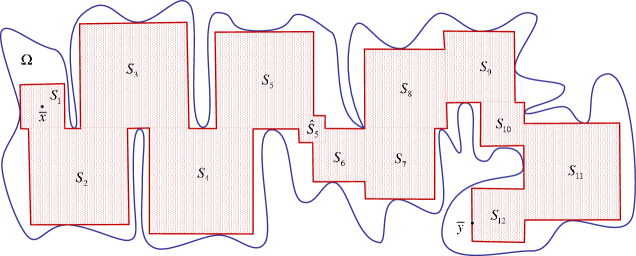
Figure 1: An example of a “Wide Path” joining $\bar{x}$ to $\bar{y}$ in $\Omega$.

The set ${\cal WP}_{\Omega}^{(\bar{x},\bar{y})}$ is an open subset of $\Omega$ possessing a number of pleasant properties which we present and prove in Sections 3. In Section 4 we study Sobolev extension properties of “The Wide Path”. The following extension theorem is the main result of that section.

Theorem 1.10

Let $p>2$ and $m\in{\bf N}$. Let $\bar{x},\bar{y}\in\Omega$ where $\Omega$ is a simply connected bounded domain in ${\bf R}^{2}$. If $\,\Omega$ is a Sobolev $L^{m}_{p}$-extension domain, then any “Wide Path” ${\mathcal{W}}={\cal WP}_{\Omega}^{(\bar{x},\bar{y})}$ joining $\bar{x}$ to $\bar{y}$ in $\Omega$ has the Sobolev $L^{m}_{p}$-extension property.

Furthermore,

$$e(L^{m}_{p}({\mathcal{W}}))\leq C\,e(L^{m}_{p}(\Omega))$$ (1.19)

where $C$ is a constant depending only on $m$ and $p$.

(See (1.2) for the definition of the indices appearing in (1.19).)

Our next step is to construct “The Narrow Path”. More specifically, in Section 5, given any “Wide Path” ${\mathcal{W}}={\cal WP}_{\Omega}^{(\bar{x},\bar{y})}$ generated from a family $\{S_{1},S_{2},...,S_{k}\}$ of squares, we prove the existence of a family ${\mathcal{Q}}_{\Omega}(\bar{x},\bar{y})=\{Q_{1},Q_{2},...,Q_{k}\}$ of pairwise disjoint squares having several “nice” properties. Let us list some of them:

(i). $Q_{1}=S_{1}$, $Q_{k}=S_{k}$, and $Q_{i}\subset S_{i}$, $1\leq i\leq k$;

(ii). $Q_{i}^{\operatorname{\,cl}}\cap Q_{i+1}^{\operatorname{\,cl}}\neq\emptyset$, $1\leq i\leq k-1$;

(iii). $\operatorname{diam}Q_{i+1}\leq 2\operatorname{dist}(Q_{i},Q_{i+2})$ provided $Q_{i}^{\operatorname{\,cl}}\cap S_{i+2}^{\operatorname{\,cl}}=\emptyset$ and $1\leq i\leq k-2$.

For additional properties of the family ${\mathcal{Q}}_{\Omega}(\bar{x},\bar{y})$ we refer the reader to Proposition 5.3.

Let

$${\cal NP}_{\Omega}^{(\bar{x},\bar{y})}:=\left(\,\bigcup_{i=1}^{k}\left(Q_{i}^{\operatorname{\,cl}}\,{\bigcup}\,\widehat{S}_{i}\,\right)\right)^{\circ}\,.$$ (1.20)

We refer to the open set ${\cal NP}_{\Omega}^{(\bar{x},\bar{y})}$ as a “Narrow Path” joining $\bar{x}$ to $\bar{y}$ in $\Omega$.

Figure 2 shows a “Narrow Path” corresponding to “The Wide Path” shown in Figure 1.

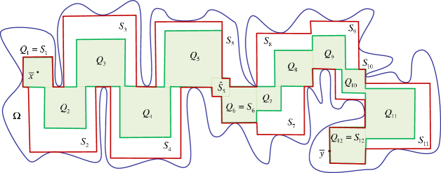
Figure 2: A “Narrow Path” joining $\bar{x}$ to $\bar{y}$ in $\Omega$.

“The Narrow Path” ${\mathcal{N}}={\cal NP}_{\Omega}^{(\bar{x},\bar{y})}$ has a simpler geometrical structure than “The Wide Path” ${\mathcal{W}}={\cal WP}_{\Omega}^{(\bar{x},\bar{y})}$. Furthermore its extension properties are similar to those of ${\cal WP}_{\Omega}^{(\bar{x},\bar{y})}$. In particular Theorem 5.11, which is proved in Section 5, states that every function $f\in L^{m}_{p}({\mathcal{N}})$ extends to a function $F\in L^{m}_{p}(\Omega)$ such that

$$\|F\|_{L^{m}_{p}(\Omega)}\leq C(m,p)\,\theta^{2}\|f\|_{L^{m}_{p}({\mathcal{N}})}$$ (1.21)

provided $\Omega$ satisfies the hypothesis of Theorem 1.8.

In Section 6 we construct the “rapidly growing” function $F_{m}$. We do this in two steps. In the first step we define a function $h_{m}$ on “The Narrow Path” ${\mathcal{N}}={\cal NP}_{\Omega}^{(\bar{x},\bar{y})}$ (see Definition 6.8). We prove that

$$D^{\beta}h_{m}(\bar{x})=0,~{}~{}~{}|\beta|=m-1,$$ (1.22)

$$\|h_{m}\|_{L^{m}_{p}({\mathcal{N}})}^{p}\leq C{\sum}_{|\beta|=m-1}|D^{\beta}h_{m}(\bar{y})|~{}~{}~{}\text{and}~{}~{}~{}d_{\alpha,\Omega}(\bar{x},\bar{y})\leq\,C{\sum}_{|\beta|=m-1}|D^{\beta}h_{m}(\bar{y})|$$ (1.23)

where $C$ is a constant depending only on $m$ and $p$. (See Proposition 6.11.)

In the second step of this procedure, using Theorem 5.11, we extend $h_{m}$ to a function $H_{m}\in L^{m}_{p}(\Omega)$ such that

$$\|H_{m}\|_{L^{m}_{p}(\Omega)}\leq C(m,p,\theta)\,\|h_{m}\|_{L^{m}_{p}({\mathcal{N}})}.$$

(See inequality (1.21).) In Proposition 6.12 we prove that properties similar to (1.22) and (1.23) also hold for the function $H_{m}$. (See (6.2), (6.3) and (6.4).)

Finally, we define the function $F_{m}$ by

$$F_{m}(u:\bar{x},\bar{y}):=\left({\sum}_{|\beta|=m-1}|D^{\beta}H_{m}(\bar{y})|\right)^{-\frac{1}{p}}\,\cdot\,H_{m}(u:\bar{x},\bar{y}),~{}~{}~{}u\in\Omega\,.$$

It can be readily seen that the above-mentioned properties of $H_{m}$ imply (1.10), (1.11) and (1.12) proving that $F_{m}$ is a “rapidly growing” function associated with $\bar{x}$ and $\bar{y}$.

This completes the proof of inequality (1.9) and therefore also the necessity part of Theorem 1.3.

Acknowledgements. We are very thankful to M. Cwikel, C. Fefferman and V. Gol’dshtein for useful suggestions and remarks. We are also very grateful to all participants of the “Whitney Problems Workshops” in Toronto, August 2012, Banff, April 2013, and Williamsburg, August 2014, for stimulating discussions and valuable advice.

2. “The Square Separation Theorem” in simply connected domains

2.1. Notation and auxiliary lemmas. Let us fix some additional notation. Throughout the paper $C,C_{1},C_{2},...$ will be generic positive constants which depend only on $m$ and $p$. These constants can change even in a single string of estimates. The dependence of a constant on certain parameters is expressed, for example, by the notation $C=C(p)$. We write $A\sim B$ if there is a constant $C\geq 1$ such that $A/C\leq B\leq CA$.

As is customary, the word “domain” means an open connected subset of ${\bf R}^{2}$. By ${\mathcal{S}}({\bf R}^{2})$ we denote the family of all open squares in ${\bf R}^{2}$ whose sides are parallel to the coordinate axis. Given a square $S\in{\mathcal{S}}({\bf R}^{2})$ by $c_{S}$ we denote its center and by $r_{S}$ half of its side length. Given $\lambda>0$ we let $\lambda\,S$ denote the dilation of $S$ with respect to its center by a factor of $\lambda$. We let $S(c,r)$ denote the square in ${\bf R}^{2}$ centered at $c$ with side length $2r$. We refer to $r=r_{S}$ as the “radius” of the square $S(c,r)$. Thus $S=S(c_{S},r_{S})$ and $\lambda S=S(c_{S},\lambda r_{S})$ for every constant $\lambda>0$.

We say that squares $S_{1}$ and $S_{2}$ are touching squares

$$\text{if}~{}~{}~{}S_{1}\cap S_{2}=\emptyset~{}~{}\text{but}~{}~{}S_{1}^{\operatorname{\,cl}}\cap S_{2}^{\operatorname{\,cl}}\neq\emptyset.$$

We denote the coordinate axes by $Oz_{1}$ and $Oz_{2}$. We also refer to the axis $Oz_{j}$ as the $z_{j}$-axis, $j=1,2$. Given $z=(z_{1},z_{2})\in{\bf R}^{2}$ by

$$\|z\|:=\max\{|z_{1}|,|z_{2}|\}$$ (2.1)

and by $\|z\|_{2}:=(|z_{1}|^{2}+|z_{2}|^{2})^{\frac{1}{2}}$ we denote the uniform and the Euclidean norms in ${\bf R}^{2}$ respectively.

Let $A,B\subset{\bf R}^{2}$. We put $\operatorname{diam}A:=\sup\{\|a-a^{\prime}\|:~{}a,a^{\prime}\in A\}$ and

$$\operatorname{dist}(A,B):=\inf\{\|a-b\|:~{}a\in A,b\in B\}.$$

Given $\varepsilon>0$ and a set $A\subset{\bf R}^{2}$ by $[A]_{\varepsilon}$ we denote the $\varepsilon$-neighborhood of $A$:

$$[A]_{\varepsilon}:=\{z\in{\bf R}^{2}:\operatorname{dist}(z,A)<\varepsilon\}.$$ (2.2)

The Lebesgue measure of a measurable set $A\subset{\bf R}^{2}$ will be denoted by $\left|A\right|$. By $\#A$ we denote the number of elements of a finite set $A$.

Let $t_{0}=0<t_{1}<t_{2}<...<t_{m}=1$, and let $\Psi:[0,1]\to{\bf R}^{2}$ be a continuous mapping which is linear on every subinterval $[t_{i},t_{i+1}]$. We refer to the curve $\gamma=\Psi([0,1])$ as a polygonal curve. Thus $\gamma$ is the union of a finite number of line segments $[\Psi(t_{i}),\Psi(t_{i+1})]$, $i=0,..,m-1$. We refer to these line segments as edges. An endpoint of an edge is called a vertex.

In what follows the word “path” will mean a polygonal curve. We say that a path is simple if it does not self intersect. We also refer to a simple closed path as a simple polygon.

Finally, for each pair of points $z_{1}$ and $z_{2}$ in ${\bf R}^{2}$ we let $[z_{1},z_{2}]$, $(z_{1},z_{2})$, $[z_{1},z_{2})$, $(z_{1},z_{2}]$ denote respectively the closed, open and semi-open line segments joining them.

Let us present several auxiliary geometrical results which we use in the sequel. First of them relates to certain properties of squares in ${\bf R}^{2}$. Recall that we measure distances in ${\bf R}^{2}$ with respect to the uniform norm in ${\bf R}^{2}$, see (2.1).

Lemma 2.1

Let $S_{1}=S(c_{1},r_{1})$ and $S_{2}=S(c_{2},r_{2})$ be squares in ${\bf R}^{2}$. Then:

(i). $S_{1}\subset S_{2}$ if and only if $r_{1}\leq r_{2}$ and $\|c_{1}-c_{2}\|\leq r_{2}-r_{1}$;

(ii). $S_{1}\cap S_{2}\neq\emptyset$ if and only if $\|c_{1}-c_{2}\|<r_{1}+r_{2}$ ;

(iii). $S_{1}$ and $S_{2}$ are touching squares if and only if $\|c_{1}-c_{2}\|=r_{1}+r_{2}$. In this case $S_{1}^{\operatorname{\,cl}}\cap S_{2}^{\operatorname{\,cl}}=\partial S_{1}\cap\partial S_{2},$ and the set $S_{1}^{\operatorname{\,cl}}\cap S_{2}^{\operatorname{\,cl}}$ is either a line segment or a point. Furthermore,

$$[c_{1},c_{2}]\cap S_{1}^{\operatorname{\,cl}}\cap S_{2}^{\operatorname{\,cl}}=\{A\}$$ (2.3)

where $A:=\alpha c_{1}+(1-\alpha)c_{2}$ with $\alpha:=r_{2}/(r_{1}+r_{2})$.

An elementary proof of the lemma we leave to the reader as an easy exercise.

The following statement is well known in geometry.

Lemma 2.2

Let $\Omega$ be a domain in ${\bf R}^{2}$.

(i). Every two point in $\Omega$ can be joined by a simple path;

(ii). Let $x,y\in\Omega$ and let $\Gamma$ be a path connecting $x$ to $y$ in $\Omega$. Then there exists a simple path $\gamma\subset\Gamma$ which joins $x$ to $y$.

We will be also needed certain well known results related to the Jordan curve theorem for polygons and certain properties of simply connected planar domains. We recall these results in the next statements. See, e.g [9] and [10].

Statement 2.3

(i). Consider a simple polygon $P$ in the plane. Its complement ${\bf R}^{2}\setminus P$ has exactly two connected components. One of these components is bounded (the interior) and the other is unbounded (the exterior), and the polygon $P$ is the boundary of each component;

(ii). Let $\Omega$ be a simply connected planar domain. Then the interior of any simple polygon $P\subset\Omega$ lies in $\Omega$.

Definition 2.4

Let $y^{\prime},y^{\prime\prime}\in{\bf R}^{2}$ and let $P\subset{\bf R}^{2}$ be a simple polygon. We say that the line segment $[y^{\prime},y^{\prime\prime}]$ strictly crosses $P$ if $[y^{\prime},y^{\prime\prime}]\cap P=\{A\}$ for some $A\in P$, and one of the following conditions is satisfied:

(i). $A$ is not a vertex of $P$;

(ii). If $A$ is a common vertex of edges $[z^{\prime},A]$ and $[A,z^{\prime\prime}]$ in the polygon $P$, then the straight line $\ell$ passing through $y^{\prime}$ and $y^{\prime\prime}$ strictly separates $z^{\prime}$ and $z^{\prime\prime}$. (I.e., $z^{\prime}$ and $z^{\prime\prime}$ lie in distinct open half-planes generated by $\ell$.)

Statement 2.5

Let $y^{\prime},y^{\prime\prime}\in{\bf R}^{2}$ and let $P\subset{\bf R}^{2}$ be a simple polygon. If $[y^{\prime},y^{\prime\prime}]$ strictly crosses $P$, then $y^{\prime}$ and $y^{\prime\prime}$ lie in distinct connected components of ${\bf R}^{2}\setminus P$.

In particular, let $\gamma$ be a simple path with ends at points $x$ and $y$. If $\gamma$ crosses $P$ exactly once at a point which is not a vertex of $P$ and not a vertex of $\gamma$, then $x$ and $y$ lie in distinct components of ${\bf R}^{2}\setminus P$.

We turn to the proof of Theorem 1.9. Its main ingredient is the following statement.

Theorem 2.6

(“The Square Separation Theorem”) Let $\Omega$ be a simply connected domain in ${\bf R}^{2}$. Let $\widetilde{S}\subset\Omega$ be a square such that

$$\partial\widetilde{S}\cap\partial\Omega\neq\emptyset.$$

Let $B\in\Omega\setminus\widetilde{S}^{\operatorname{\,cl}}$. Then there exists a square $Q\subset\Omega\setminus\widetilde{S}^{\operatorname{\,cl}}$ satisfying the following conditions:

(i). $Q^{\operatorname{\,cl}}\cap\widetilde{S}^{\operatorname{\,cl}}\cap\Omega\neq\emptyset$;

(ii). Either $B\in Q^{\operatorname{\,cl}}$ or

$$\widetilde{S}~{}~{}\text{and}~{}~{}B~{}~{}\text{lie in different connected components of}~{}~{}\Omega\setminus Q^{\operatorname{\,cl}}.$$ (2.4)

See Figure 3.

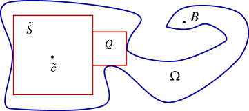
Figure 3:  

In the sequel we let $\tilde{c}$ and $R$ denote the center and the “radius” of $\widetilde{S}$ respectively; thus

$$\widetilde{S}=S(\tilde{c},R).$$

The proof of Theorem 2.6 relies on a series of auxiliary results. Towards their formulation let us introduce several definitions and notations.

Definition 2.7

Fix a point $w\in\partial\widetilde{S}\cap\partial\Omega$. By $\prec$ we denote the total ordering on the set $\partial\widetilde{S}\setminus\{w\}$ induced by the clockwise direction on $\partial\widetilde{S}$.

Given $a,b\in\partial\widetilde{S}\setminus\{w\}$, $a\neq b$, we define the open interval $(a,b)_{\partial\widetilde{S}}$, closed interval $[a,b]_{\partial\widetilde{S}}$ and semi-open intervals $(a,b]_{\partial\widetilde{S}}$ and $[a,b)_{\partial\widetilde{S}}$ by letting

$$(a,b)_{\partial\widetilde{S}}=\{x\in\partial\widetilde{S}\setminus\{w\}:a\prec x\prec b,\,x\neq a,b\},$$

$[a,b]_{\partial\widetilde{S}}=(a,b)_{\partial\widetilde{S}}\cup\{a,b\}$ and $(a,b]_{\partial\widetilde{S}}=(a,b)_{\partial\widetilde{S}}\cup\{b\}$, $[a,b)_{\partial\widetilde{S}}=(a,b)_{\partial\widetilde{S}}\cup\{a\}.$

In particular, every connected component ${\mathcal{T}}$ of $\partial\widetilde{S}\setminus\partial\Omega=\partial\widetilde{S}\cap\Omega$ is an open interval in $\partial\widetilde{S}\setminus\{w\}$, completely determined by its beginning $b_{\mathcal{T}}$ and its end $e_{\mathcal{T}}$. Thus $b_{\mathcal{T}},e_{\mathcal{T}}\in\partial\widetilde{S}\cap\partial\Omega$, $b_{\mathcal{T}}\prec e_{\mathcal{T}}$ and ${\mathcal{T}}=(b_{\mathcal{T}},e_{\mathcal{T}})_{\partial\widetilde{S}}$ .

It is also clear that for every two distinct connected components ${\mathcal{T}}_{0}$ and ${\mathcal{T}}_{1}$ of $\partial\widetilde{S}\setminus\partial\Omega$ either $e_{{\mathcal{T}}_{0}}\prec b_{{\mathcal{T}}_{1}},$ or $e_{{\mathcal{T}}_{1}}\prec b_{{\mathcal{T}}_{0}}$. We also notice the following important properties of the components ${\mathcal{T}}_{0}$ and ${\mathcal{T}}_{1}$:

$$(e_{{\mathcal{T}}_{0}},b_{{\mathcal{T}}_{1}})_{\partial\widetilde{S}}\cap\partial\Omega\neq\emptyset~{}~{}~{}\text{provided}~{}~{}~{}e_{{\mathcal{T}}_{0}}\prec b_{{\mathcal{T}}_{1}}.$$

Lemma 2.8

(i). Let $G$ be a connected component of $\Omega\setminus\widetilde{S}^{\operatorname{\,cl}}$. There exists a unique connected component ${\mathcal{T}}={\mathcal{T}}(G)$ of $\partial\widetilde{S}\setminus\partial\Omega$ having the following property:

$$\text{Every}~{}x\in G~{}\text{and every}~{}y\in{\mathcal{T}}~{}\text{can be joined by a path}~{}~{}\gamma~{}\text{such that}~{}\gamma\setminus\{y\}\subset G$$ (2.5)

(ii). For every connected component ${\mathcal{T}}$ of $\partial\widetilde{S}\setminus\partial\Omega$ there exists a unique connected component $G$ of $\Omega\setminus\widetilde{S}^{\operatorname{\,cl}}$ which satisfies condition (2.5).

Proof. First we prove the following

Statement A: Let $G$ be a connected component of $\Omega\setminus\widetilde{S}^{\operatorname{\,cl}}$ and let ${\mathcal{T}}$ be a connected component of $\partial\widetilde{S}\setminus\partial\Omega$. Let $x_{0}\in G$ and let $p_{0}\in{\mathcal{T}}$. Suppose that

$$\text{there exists a path}~{}~{}\gamma_{0}~{}~{}\text{which joins}~{}~{}x_{0}~{}~{}\text{to}~{}~{}p_{0}~{}~{}\text{such that}~{}~{}\gamma_{0}\setminus\{p_{0}\}\subset G.$$ (2.6)

Then condition (2.5) holds.

Let us prove this statement. Since every $x\in G$ can be connected to $x_{0}$ by a path in $G$, to prove (2.5) it suffices to show that for each $y\in{\mathcal{T}}$ there exists a path $\gamma$ which joins $x_{0}$ to $y$ such that $\gamma\setminus\{y\}\subset G$.

Without loss of generality we can assume that $p_{0}$ and $y$ belong to the same side of the square $\widetilde{S}$. In other words, we can assume that $I:=[p_{0},y]\subset{\mathcal{T}}$. Since $I$ is a compact subset of $\Omega$, we have $\varepsilon:=\operatorname{dist}(I,\partial\Omega)/2>0$.

Recall that $[I]_{\varepsilon}$ denotes the $\varepsilon$-neighborhood of $I$, see (2.2). Then, by definition, $[I]_{\varepsilon}\subset\Omega$. Furthermore, the set $D_{\varepsilon}:=[I]_{\varepsilon}\setminus\widetilde{S}^{\operatorname{\,cl}}$ is an open rectangle.

Since $\gamma_{0}$ is a continuous curve which joins $x_{0}$ to $p_{0}$, there exists a point $\widetilde{p}\in\gamma_{0}\cap[I]_{\varepsilon}$. Since $\gamma_{0}\setminus\{p_{0}\}\subset G\subset\Omega\setminus\widetilde{S}^{\operatorname{\,cl}}$, we conclude that $\widetilde{p}\in D_{\varepsilon}$. Let $\gamma_{1}:=[\widetilde{p},y]$ and let $\gamma_{2}$ be the union of $\gamma_{1}$ and the subarc of $\gamma_{0}$ from $x_{0}$ to $\widetilde{p}$. Since the rectangle $D_{\varepsilon}$ is convex, $\gamma_{1}\setminus\{y\}\subset D_{\varepsilon}\subset\Omega$ so that $\gamma_{2}\setminus\{y\}\subset\Omega$. Since $x_{0}\in\gamma_{2}$ we conclude that $\gamma_{2}\setminus\{y\}\subset G$ proving Statement A.

Let us prove part (i) of the lemma. Fix a point $x_{0}\in G$. By $\gamma_{0}$ we denote a path in $\Omega$ which connects $x_{0}$ to the point $\tilde{c}$, the center of the square $\widetilde{S}$. See Lemma 2.2.

Since $x_{0}\notin\widetilde{S}^{\operatorname{\,cl}}$ and $\tilde{c}\in\widetilde{S}^{\operatorname{\,cl}}$, there exists a point

$$p_{0}\in\partial\widetilde{S}\setminus\partial\Omega=\partial\widetilde{S}\cap\Omega$$

such that $\gamma_{0}\setminus\{p_{0}\}\subset G$. Let ${\mathcal{T}}={\mathcal{T}}(G)$ be a connected component of $\partial\widetilde{S}\setminus\partial\Omega$ which contains $p_{0}$. Since condition (2.6) is satisfied, by Statement A, condition (2.5) holds.

Prove the uniqueness of the component ${\mathcal{T}}={\mathcal{T}}(G)$. Suppose that the set $\partial\widetilde{S}\setminus\partial\Omega$ contains two distinct connected components, ${\mathcal{T}}^{\prime}$ and ${\mathcal{T}}^{\prime\prime}$, ${\mathcal{T}}^{\prime}\neq{\mathcal{T}}^{\prime\prime}$, such that for every $x\in G$ and every $y^{\prime}\in{\mathcal{T}}^{\prime},y^{\prime\prime}\in{\mathcal{T}}^{\prime\prime}$ there exist paths $\gamma^{\prime}$ and $\gamma^{\prime\prime}$ joining $x$ to $y^{\prime}$ and $y^{\prime\prime}$ respectively such that

$$\gamma^{\prime}\setminus\{y^{\prime}\}\subset G~{}~{}~{}\text{and}~{}~{}~{}\gamma^{\prime\prime}\setminus\{y^{\prime\prime}\}\subset G.$$ (2.7)

Fix a point $\bar{x}\in G$ and points $p^{\prime}\in{\mathcal{T}}^{\prime}$ and $p^{\prime\prime}\in{\mathcal{T}}^{\prime\prime}$. Without loss of generality we can assume that $p^{\prime}\prec p^{\prime\prime}$. Let

$$V_{0}:=(p^{\prime},p^{\prime\prime})_{\partial\widetilde{S}}~{}~{}~{}\text{and}~{}~{}~{}V_{1}:=\partial\widetilde{S}\setminus[p^{\prime},p^{\prime\prime}]_{\partial\widetilde{S}}.$$

Then $V_{0}\cup V_{1}=\partial\widetilde{S}\setminus\{p^{\prime},p^{\prime\prime}\}$.

Since $p^{\prime}\in{\mathcal{T}}^{\prime}$, $p^{\prime\prime}\in{\mathcal{T}}^{\prime\prime}$ and ${\mathcal{T}}^{\prime}\neq{\mathcal{T}}^{\prime\prime}$, we have $V_{0}\nsubseteq\Omega$. In fact, if $V_{0}\subset\Omega$, then $p^{\prime}$ and $p^{\prime\prime}$ belong to the same connected component of $\partial\widetilde{S}\setminus\partial\Omega$ so that ${\mathcal{T}}^{\prime}={\mathcal{T}}^{\prime\prime}$, a contradiction. In the same way we prove that $V_{1}\nsubseteq\Omega$.

Thus there exist points $y_{0}\in V_{0}\setminus\Omega$ and $y_{1}\in V_{1}\setminus\Omega$. Prove that the existence of these points leads us to a contradiction. By (2.7), there exist paths $\Gamma^{\prime}$ and $\Gamma^{\prime\prime}$ which connects $\bar{x}$ to $p^{\prime}$ and $p^{\prime\prime}$ respectively, and such that the sets $\Gamma^{\prime}\setminus\{p^{\prime}\}$ and $\Gamma^{\prime\prime}\setminus\{p^{\prime\prime}\}$ lie in $G$. Hence $\Gamma:=\Gamma^{\prime}\cup\Gamma^{\prime\prime}$ is a path which joins $p^{\prime}$ to $p^{\prime\prime}$ such that $\Gamma\setminus\{p^{\prime},p^{\prime\prime}\}\subset G$.

By part (ii) of Lemma 2.2, there exists a simple path $\gamma_{1}\subset\Gamma$ which connects $p^{\prime}$ to $p^{\prime\prime}$. Hence, $\gamma_{1}\setminus\{p^{\prime},p^{\prime\prime}\}\subset G$ so that $\gamma_{1}\setminus\{p^{\prime},p^{\prime\prime}\}\subset{\bf R}^{2}\setminus\widetilde{S}^{\operatorname{\,cl}}$.

Let $\gamma_{2}:=[p^{\prime},\tilde{c}]$ and let $\gamma_{3}:=[\tilde{c},p^{\prime\prime}]$. Then the loop $\widetilde{\gamma}:=\gamma_{1}\cup\gamma_{2}\cup\gamma_{3}$ is a simple closed path in $\Omega$, i.e., $\widetilde{\gamma}$ is a simple polygon. See Figure 4.

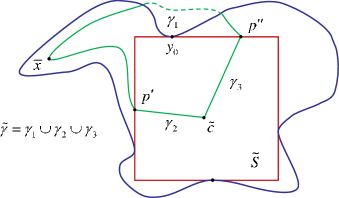
Figure 4: $p^{\prime}\in{\mathcal{T}}^{\prime},p^{\prime\prime}\in{\mathcal{T}}^{\prime\prime}$ and $\gamma_{1}$ joins $p^{\prime}$ to $p^{\prime\prime}$ in ${\bf R}^{2}\setminus\widetilde{S}^{\operatorname{\,cl}}$.

By the Jordan curve theorem, see part (i) of Statement 2.3, the complement of $\widetilde{\gamma}$, the set ${\bf R}^{2}\setminus\widetilde{\gamma}$, consists of exactly two connected components - the interior component (which is a bounded set), and the exterior component (which is an unbounded set). We denote these components by $D_{int}$ and $D_{ext}$ respectively. The polygon $\widetilde{\gamma}$ is the boundary of these domains, i.e.,

$$\widetilde{\gamma}=\partial D_{int}=\partial D_{ext}.$$

Furthermore, since $\Omega$ is a simply connected domain and $\widetilde{\gamma}\subset\Omega$ is a simple polygon, by part (ii) of Statement 2.3,

$$D_{int}\subset\Omega.$$ (2.8)

Clearly, there exists a polygonal path $\gamma^{\prime}$ (with at most two edges) which joins $y_{0}$ to $y_{1}$ in $\widetilde{S}$ and crosses $(p^{\prime},\tilde{c}]\cup[\tilde{c},p^{\prime\prime})$ exactly once at a point which is not $\tilde{c}$ or a vertex of $\gamma^{\prime}$. Since

$$\gamma_{1}\setminus\{p^{\prime},p^{\prime\prime}\}\subset{\bf R}^{2}\setminus\widetilde{S}^{\operatorname{\,cl}},$$

the path $\gamma^{\prime}$ has no common points with $\gamma_{1}$, so that $\gamma^{\prime}$ crosses the simple polygon

$$\widetilde{\gamma}:=\gamma_{1}\cup\gamma_{2}\cup\gamma_{3}$$

exactly once at a point which is not a vertex of $\widetilde{\gamma}$ or $\gamma^{\prime}$. Hence, by Statement 2.5, the points $y_{0}$ and $y_{1}$ lie in different components of ${\bf R}^{2}\setminus\widetilde{\gamma}$.

Thus the component $D_{int}$ contains either $y_{0}$ or $y_{1}$. But $y_{0},y_{1}\in{\bf R}^{2}\setminus\Omega$ so that $D_{int}\nsubseteq\Omega$. On the other hand, by (2.8), $D_{int}\subset\Omega$. We have obtained a contradiction which proves part (i) of the lemma.

Prove (ii). Let ${\mathcal{T}}$ be a connected component of $\partial\widetilde{S}\setminus\partial\Omega$ and let $p_{0}\in{\mathcal{T}}$. Since the point $p_{0}\in\partial\widetilde{S}\setminus\partial\Omega=\partial\widetilde{S}\cap\Omega$, for an $\varepsilon>0$ small enough the square $S(p_{0},\varepsilon)\subset\Omega$. Clearly,

$$J_{\varepsilon}:=S(p_{0},\varepsilon)\setminus\widetilde{S}^{\operatorname{\,cl}}$$

is a non-empty connected set. Also there exists a point $x_{0}\in J_{\varepsilon}$ such that the line segment $[x_{0},p_{0})\subset J_{\varepsilon}$.

Let $G$ be a connected component of $\Omega\setminus\widetilde{S}^{\operatorname{\,cl}}$ which contains $x_{0}$, and let $\gamma_{0}:=[x_{0},p_{0}]$. Since $J_{\varepsilon}$ is a connected subset of $\Omega\setminus\widetilde{S}^{\operatorname{\,cl}}$ containing $x_{0}$, we have $J_{\varepsilon}\subset G$. Hence $\gamma_{0}\setminus\{p_{0}\}\subset G$ so that condition (2.6) is satisfied. On the other hand, by Statement A, condition (2.6) implies (2.5) proving the existence of a connected component $G$ satisfying part (ii) of the lemma.

This proof also enables us to show the uniqueness of the component $G$. In fact, let $G^{\prime}$ be a connected component of $\Omega\setminus\widetilde{S}^{\operatorname{\,cl}}$ such that any $x\in G^{\prime}$ and any $y\in{\mathcal{T}}$ can be joined by a path $\gamma$ with $\gamma\setminus\{y\}\subset G^{\prime}$. Let $\gamma$ be such a path which connects $x\in G^{\prime}$ to $y=p_{0}$. Since $\gamma$ is a continuous curve, there exists a point $z\in\gamma\cap S(p_{0},\varepsilon)$. But $\gamma\subset\Omega\setminus\widetilde{S}^{\operatorname{\,cl}}$ so that

$$z\in S(p_{0},\varepsilon)\setminus\widetilde{S}^{\operatorname{\,cl}}=J_{\varepsilon}.$$

The proof of the lemma is complete.         $\Box$

Lemma 2.8 shows that ${\mathcal{T}}={\mathcal{T}}(G)$ is a one-to-one mapping between the families of connected components of $\Omega\setminus\widetilde{S}^{\operatorname{\,cl}}$ and the families of connected components of $\partial\widetilde{S}\setminus\partial\Omega$.

We let ${\mathcal{G}}$ denote the mapping which is inverse to ${\mathcal{T}}(G)$. Thus for every connected component ${\mathcal{T}}$ of $\partial\widetilde{S}\setminus\partial\Omega$ the set $G={\mathcal{G}}({\mathcal{T}})$ is the (unique) connected component of $\Omega\setminus\widetilde{S}^{\operatorname{\,cl}}$ such that (2.5) is satisfied.

We also notice a simple connection between ${\mathcal{T}}$ and $G={\mathcal{G}}({\mathcal{T}})$:

$${\mathcal{T}}(G)=\partial G\setminus\partial\Omega=\partial G\cap\Omega.\vskip 3.0pt plus 1.0pt minus 1.0pt$$

We turn to the next step of the proof of Theorem 2.6.

2.2. A parameterized family of separating squares and its main properties.

Definition 2.9

Let $B\in\Omega\setminus\widetilde{S}^{\operatorname{\,cl}}$. By $G_{B}$ we denote the connected component of $\Omega\setminus\widetilde{S}^{\operatorname{\,cl}}$ containing $B$, and by ${\mathcal{T}}_{B}={\mathcal{T}}(G_{B})$ we denote the corresponding connected component of $\partial\widetilde{S}\setminus\partial\Omega$ associated with $G_{B}$. We represent ${\mathcal{T}}_{B}$ in the form ${\mathcal{T}}=(b_{{\mathcal{T}}_{B}},e_{{\mathcal{T}}_{B}})_{\partial\widetilde{S}}$ where $b_{{\mathcal{T}}_{B}},e_{{\mathcal{T}}_{B}}\in\partial\widetilde{S}$, $b_{{\mathcal{T}}_{B}}\prec e_{{\mathcal{T}}_{B}}$. See Definition 2.7.

By Lemma 2.8, the component ${\mathcal{T}}_{B}$ is well defined.

Our aim at this step of the proof is to introduce a certain parametrization of squares touching the square $\widetilde{S}=S(\tilde{c},R)$ and lying in $G_{B}$. Let $z\in\partial\widetilde{S}$ and let $r>0$. By $K_{r}(z)$ we denote a square with “radius” $r$ and center

$$z_{r}:=z+\tfrac{r}{R}(z-\tilde{c}).$$

Since $\|z-\tilde{c}\|=R$, we have

$$\|z_{r}-\tilde{c}\|=\|z+\tfrac{r}{R}(z-\tilde{c})-\tilde{c}\|=(1+\tfrac{r}{R})\|z-\tilde{c}\|=R+r$$

so that, by part (iii) of Lemma 2.1,

$$K_{r}(z)~{}~{}\text{and}~{}~{}\widetilde{S}~{}~{}\text{are touching squares}.$$ (2.9)

Furthermore, if $0<r_{1}\leq r_{2}$, then

$$\|z_{r_{1}}-z_{r_{2}}\|=\|z+\tfrac{r_{1}}{R}(z-\tilde{c})-(z+\tfrac{r_{2}}{R}(z-\tilde{c}))\|=r_{2}-r_{1}.$$

Therefore, by part (i) of Lemma 2.1,

$$K_{r_{1}}(z)\subset K_{r_{2}}(z)~{}~{}~{}\text{whenever}~{}~{}~{}0<r_{1}\leq r_{2}$$

proving that the family of squares $\{K_{r}(z):r>0\}$ is ordered with respect to inclusion. This motivates us to introduces the following

Definition 2.10

Let $z\in{\mathcal{T}}_{B}$. By $K(z)$ we denote the maximal (with respect to inclusion) element of the family of squares

$${\mathcal{K}}(z):=\{K_{r}(z):r>0,K_{r}(z)\subset\Omega\}.$$

We let $c_{z}$ and $r_{z}$ denote the center and the “radius” of $K(z)$ respectively.

Thus $K(z)$ is the square of the maximal diameter belonging to the family of squares ${\mathcal{K}}(z)$. It can be represented in the form

$$K(z)=S(c_{z},r_{z}),~{}~{}~{}z\in{\mathcal{T}}_{B}$$

where

$$c_{z}=z+\tfrac{r_{z}}{R}(z-\tilde{c}).$$ (2.10)

See Figure 5.

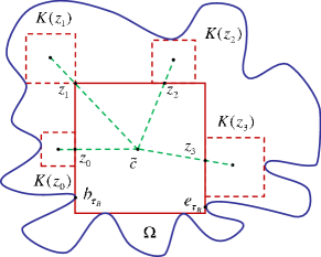
Figure 5: Examples of squares $K(z_{i})$, $i=0,...3.$

Let us describe several simple properties of the squares $K(z),z\in{\mathcal{T}}_{B}$.

Lemma 2.11

Let $z\in{\mathcal{T}}_{B}$.

(a). The square $K(z)$ is well defined;

(b). $K(z)$ and $\widetilde{S}$ are touching squares such that $K(z)^{\operatorname{\,cl}}\cap\partial\widetilde{S}\cap\Omega\neq\emptyset$;

(c). $K(z)\subset\Omega\setminus\widetilde{S}^{\operatorname{\,cl}}$ and $\operatorname{dist}(K(z),\partial\Omega\setminus\partial\widetilde{S})=0$ ;

(d). The line segment $[\tilde{c},c_{z}]$ lies in $\Omega$:

$$[\tilde{c},c_{z}]\subset\Omega.$$ (2.11)

Furthermore,

$$z\in K(z)^{\operatorname{\,cl}}\cap\widetilde{S}^{\operatorname{\,cl}}\cap\Omega\,;$$ (2.12)

(e). For every $u\in K(z)^{\operatorname{\,cl}}\cap\Omega$ there exists a path $\gamma$ which joins $u$ to $B$ in $\Omega$ such that $(\gamma\setminus\{u\})\cap\widetilde{S}^{\operatorname{\,cl}}=\emptyset$.

In particular, this implies that $K(z)$ and $B$ belong to the same connected component of  $\Omega\setminus\widetilde{S}^{\operatorname{\,cl}}$ (i.e., the component $G_{B}$).

Proof. Since $\Omega$ is a bounded domain and $K(z)$ is the square of the maximal diameter from the family ${\mathcal{K}}(z)$, this square is well defined. This proves (a).

In turn, property (b) follows from (2.9), and property (c) from the maximality of the square $K(z)$. Property (d) follows from the fact that the point $z\in{\mathcal{T}}_{B}\subset\Omega$ and $\widetilde{S}\cup K(z)\subset\Omega$.

Prove (e). Since $z\in{\mathcal{T}}_{B}$, by Definition 2.9 and Lemma 2.8, there exists a path $\gamma_{z}$ which joins $B$ to $z$ in $\Omega$ such that $\gamma_{z}\setminus\{z\}\subset G_{B}$. Recall that $z\in\Omega$ so that for some $\varepsilon>0$ small enough the $\varepsilon$-neighborhood of $z$, the square $S(z,\varepsilon)\subset\Omega$.

Clearly, $(\gamma_{z}\setminus\{z\})\cap S(z,\varepsilon)\neq\emptyset$ and $K(z)\cap S(z,\varepsilon)\neq\emptyset$ so that there exist points $a\in\gamma\setminus\{z\}$, and $b\in K(z)$ which belong to $S(z,\varepsilon)$.

Let $\gamma_{1}$ be the arc of $\gamma$ from $B$ to $a$. Clearly, $S(z,\varepsilon)\setminus\widetilde{S}^{\operatorname{\,cl}}$ is an open connected set so that there exists a path $\gamma_{2}$ in $S(z,\varepsilon)\setminus\widetilde{S}^{\operatorname{\,cl}}$ joining $a$ to $b$. Finally, let $\gamma_{3}:=[b,u]$.

Let $\gamma:=\gamma_{1}\cup\gamma_{2}\cup\gamma_{3}$. Then $\gamma$ is a path which joins $u$ to $B$ in $\Omega$. Since

$$\gamma_{1}\cap\widetilde{S}^{\operatorname{\,cl}}=\gamma_{2}\cap\widetilde{S}^{\operatorname{\,cl}}=\emptyset,$$

$b\in K(z)$ and $u\in K(z)^{\operatorname{\,cl}}\cap\Omega$, the path $\gamma\setminus\{u\}$ does not intersect $\widetilde{S}^{\operatorname{\,cl}}$.

Prove the second statement of part (e). Since $K(z)\cap\widetilde{S}^{\operatorname{\,cl}}=\emptyset$, we conclude that every point $u\in K(z)$ can be joined to $B$ by a path $\gamma\subset\Omega$ such that $\gamma\cap\widetilde{S}^{\operatorname{\,cl}}=\emptyset$. Clearly, this implies that $K(z)$ and $B$ belong to the same connected component of  $\Omega\setminus\widetilde{S}^{\operatorname{\,cl}}$.

The lemma is proved.         $\Box$

Lemma 2.12

Let $z,y\in{\mathcal{T}}_{B},z\neq y$. Suppose that $z$ and $y$ lie on a side $[a,b]$ of the square $\widetilde{S}$.

(i). If $z,y\in(a,b)$, then

$$|r_{y}-r_{z}|\leq\frac{(R+r_{y}+r_{z})\,\|y-z\|}{\operatorname{dist}(\{z,y\},\{a,b\})}\,;$$

(ii). If $z\in\{a,b\}$ and $y\in(a,b)$, then

$$r_{y}\leq r_{z}+\frac{(R+r_{z})\,\|y-z\|}{\|y-h\|}$$

where $h:=\{a,b\}\setminus\{z\}$.

Proof. Without loss of generality we may assume that $\tilde{c}=(0,-R)$, $a=(-R,0)$ and $b=(R,0)$. See Figure 6.

Figure 6:  

Since $y,z\in[a,b]\subset Ox$, we have $y=(y_{1},0)$ and $z=(z_{1},0)$ where $|y_{1}|\leq R$ and $|z_{1}|\leq R$. Since $K(z)$ and $\widetilde{S}$ are touching squares, intersection of $K(z)^{\operatorname{\,cl}}$ with the axis $Ox$ is a closed line segment which coincides with a side of $K(z)$. Let $(a_{z},0)\in Ox$ and $(b_{z},0)\in Ox$ be the ends of this side so that

$$K(z)^{\operatorname{\,cl}}\cap Ox=[(a_{z},0),(b_{z},0)].$$ (2.13)

In the same way we define points $(a_{y},0),(b_{y},0)\in Ox$; thus

$$K(y)^{\operatorname{\,cl}}\cap Ox=[(a_{y},0),(b_{y},0)].$$

Let us give explicit formulae for these points. By (2.10),

$$c_{z}=z+\tfrac{r_{z}}{R}(z-\tilde{c})=\left(z_{1}\left(1+\tfrac{r_{z}}{R}\right),r_{z}\right)$$

so that

$$a_{z}=z_{1}\left(1+\tfrac{r_{z}}{R}\right)-r_{z}~{}~{}~{}\text{and}~{}~{}~{}b_{z}=z_{1}\left(1+\tfrac{r_{z}}{R}\right)+r_{z}.$$ (2.14)

In the same way we obtain formulae for $a_{y}$ and $b_{y}$:

$$a_{y}=y_{1}\left(1+\tfrac{r_{y}}{R}\right)-r_{y}~{}~{}~{}\text{and}~{}~{}~{}b_{y}=y_{1}\left(1+\tfrac{r_{y}}{R}\right)+r_{y}.$$ (2.15)

Prove that either

$$a_{y}\leq a_{z}~{}~{}~{}\text{and}~{}~{}~{}b_{y}\leq b_{z}$$ (2.16)

or

$$a_{z}\leq a_{y}~{}~{}~{}\text{and}~{}~{}~{}b_{z}\leq b_{y}\,.$$ (2.17)

In fact, assume that both (2.16) and (2.17) do not hold. Then either

$$a_{y}<a_{z}~{}~{}~{}\text{and}~{}~{}~{}b_{z}<b_{y}$$ (2.18)

or

$$a_{z}<a_{y}~{}~{}~{}\text{and}~{}~{}~{}b_{y}<b_{z}\,.$$ (2.19)

Prove that (2.18) contradicts the maximality of the square $K(z)$. In fact, if (2.18) holds, then $K(z)^{\operatorname{\,cl}}\subset K(y)$ so that $K(z)^{\operatorname{\,cl}}\subset\Omega$. But this inclusion contradicts the equality

$$\operatorname{dist}(K(z),\partial\Omega\setminus\partial\widetilde{S})=0,$$

see part (c) of Lemma 2.11. In the same way we show that (2.19) is not true proving that either (2.16) or (2.17) holds.

We are in a position to prove part (i) of the lemma. Suppose that $y,z\in(a,b)$ and the option (2.16) holds. By (2.14) and (2.15), inequality $a_{y}\leq a_{z}$ is equivalent to the inequality

$$y_{1}\left(1+\tfrac{r_{y}}{R}\right)-r_{y}\leq z_{1}\left(1+\tfrac{r_{z}}{R}\right)-r_{z}.$$

Hence

$$r_{y}-r_{z}\geq\frac{(R+r_{z})(y_{1}-z_{1})}{R-y_{1}}\,.$$

In turn, inequality $b_{y}\leq b_{z}$ implies that

$$r_{y}-r_{z}\leq\frac{(R+r_{z})(z_{1}-y_{1})}{R+y_{1}}\,.$$ (2.20)

In the same way we prove that (2.17) implies the following:

$$r_{z}-r_{y}\geq\frac{(R+r_{y})(z_{1}-y_{1})}{R-z_{1}}~{}~{}\text{and}~{}~{}r_{z}-r_{y}\leq\frac{(R+r_{y})(y_{1}-z_{1})}{R+y_{1}}\,.$$

Summarizing these estimates, we obtain

$$|r_{y}-r_{z}|\leq|y_{1}-z_{1}|\,\max\left\{\frac{R+r_{z}}{R+y_{1}},\frac{R+r_{y}}{R+z_{1}},\frac{R+r_{z}}{R-y_{1}},\frac{R+r_{y}}{R-z_{1}}\right\}\,.$$

But $|y_{1}-z_{1}|=\|y-z\|$ so that

$$|r_{y}-r_{z}|\leq\frac{\|y-z\|\,(R+r_{y}+r_{z})}{\min\{R+y_{1},R-y_{1},R+z_{1},R-z_{1}\}}=\frac{\|y-z\|\,(R+r_{y}+r_{z})}{\operatorname{dist}\{\{y,z\},\{a,b\}\}}$$

proving part (i) of the lemma.

Prove (ii). Let $z=b$ and let $y\in(a,b)$ so that $z_{1}=R$ and $-R<y_{1}<R$. By (2.14) and (2.15),

$$a_{y}=y_{1}\left(1+\tfrac{r_{y}}{R}\right)-r_{y}=y_{1}+r_{y}\left(\tfrac{y_{1}}{R}-1\right)<y_{1}$$

and

$$a_{z}=z_{1}\left(1+\tfrac{r_{z}}{R}\right)-r_{z}=R\left(1+\tfrac{r_{z}}{R}\right)-r_{z}=R$$

so that $a_{y}<a_{z}$. Therefore, by (2.16), $b_{y}\leq b_{z}$. Hence, by (2.20),

$$r_{y}-r_{z}\leq\frac{(R+r_{z})(z_{1}-y_{1})}{R+y_{1}}=\frac{(R+r_{z})\|y-z\|}{R+y_{1}}\,.$$

Since $a=(-R,0)$ and $y=(y_{1},0)$, we have $R+y_{1}=\|y-a\|$ proving part (ii) of the lemma in the case under consideration. In the same fashion we prove (ii) whenever $z=a$.

The proof of the lemma is complete.         $\Box$

Lemma 2.13

Let $z\in{\mathcal{T}}_{B}$ and let $\varepsilon>0$. There exists $\delta>0$ such that for every $y\in{\mathcal{T}}_{B}$, $\|y-z\|<\delta$, the following inclusion

$$K(y)\subset[K(z)]_{\varepsilon}$$ (2.21)

holds. Recall that the symbol $[\,\,\cdot\,\,]_{\varepsilon}$ denotes the $\varepsilon$-neighborhood of a set.

Proof. Clearly, $[K(z)]_{\varepsilon}$ is a square with center $c_{z}$ and “radius” $r_{z}+\varepsilon$, i.e.,

$$[K(z)]_{\varepsilon}=S(c_{z},r_{z}+\varepsilon).$$

By part (i) of Lemma 2.1, inclusion (2.21) is equivalent to the inequality

$$\|c_{y}-c_{z}\|+r_{y}\leq r_{z}+\varepsilon.$$ (2.22)

Let us consider two cases.

The first case: $z$ is not a vertex of the square $\widetilde{S}$, i.e.,

$$\tau:=\operatorname{dist}(z,V_{{\mathcal{T}}_{B}})>0.$$

Here $V_{{\mathcal{T}}_{B}}$ is the family of vertices of $\widetilde{S}$ which belong to ${\mathcal{T}}_{B}$. In particular, every point $y\in{\mathcal{T}}_{B}$ such that $\|y-z\|<\tau/2$ belongs to the same side of $\widetilde{S}$ as the point $z$. Furthermore,

$$\operatorname{dist}(y,V_{{\mathcal{T}}_{B}})\geq\tau/2>0.$$ (2.23)

By part (i) of Lemma 2.12,

$$|r_{y}-r_{z}|\leq\frac{(R+r_{y}+r_{z})\|y-z\|}{\operatorname{dist}(\{y,z\},V_{{\mathcal{T}}_{B}})}$$

so that, by (2.23),

$$|r_{y}-r_{z}|\leq(2/\tau)(R+r_{y}+r_{z})\|y-z\|=\gamma_{1}\|y-z\|$$

where $\gamma_{1}:=2(R+r_{y}+r_{z})/\tau$.

By (2.10),

$$c_{z}=z+\tfrac{r_{z}}{R}(z-\tilde{c})~{}~{}~{}\text{and}~{}~{}~{}c_{y}=y+\tfrac{r_{y}}{R}(y-\tilde{c})$$

so that

$$\|c_{y}-c_{z}\|\leq\|y-z\|+\tfrac{|r_{y}-r_{z}|}{R}\|z-\tilde{c}\|+\tfrac{r_{y}}{R}\|y-z\|\,.$$

Since $\|z-\tilde{c}\|=R$, we obtain

$$\|c_{y}-c_{z}\|\leq\left(1+\tfrac{r_{y}}{R}\right)\|y-z\|+|r_{y}-r_{z}|\,.$$ (2.24)

Hence,

$$\|c_{y}-c_{z}\|\leq\left(1+\tfrac{r_{y}}{R}+\gamma_{1}\right)\|y-z\|=\gamma_{2}\|y-z\|$$

with $\gamma_{2}:=1+\tfrac{r_{y}}{R}+\gamma_{1}$.

Now we are in a position to estimate the left-hand side of (2.22):

$$\|c_{y}-c_{z}\|+r_{y}\leq\|c_{y}-c_{z}\|+|r_{y}-r_{z}|+r_{z}\leq\gamma_{2}\|y-z\|+\gamma_{1}\|y-z\|+r_{z}=(\gamma_{1}+\gamma_{2})\|y-z\|+r_{z}.$$

This proves that whenever $\|y-z\|<\delta$ with $\delta:=\min\{\tau/2,\varepsilon/(\gamma_{1}+\gamma_{2})\}$ the inequality (2.22) holds.

The second case: $z$ is a vertex of $\widetilde{S}$. Let $y\in{\mathcal{T}}_{B}$, $\|y-z\|<R/2$. Hence, $\|y-a\|>R/2$ for every vertex $a$ of $\widetilde{S}$, $a\neq z$. Then, by part (ii) of Lemma 2.12,

$$r_{y}\leq r_{z}+\frac{(R+r_{z})\,\|y-z\|}{(R/2)}=r_{z}+2(1+r_{z}/R)\,\|y-z\|\,.$$ (2.25)

Prove inequality (2.22). If $r_{z}\geq r_{y}$, then, by (2.24),

$$\|c_{y}-c_{z}\|+r_{y}\leq\left(1+\tfrac{r_{y}}{R}\right)\|y-z\|+|r_{z}-r_{y}|+r_{y}=\left(1+\tfrac{r_{y}}{R}\right)\|y-z\|+r_{z}\,.$$ (2.26)

If $r_{z}<r_{y}$, then, by (2.24) and (2.25),

$$\|c_{y}-c_{z}\|+r_{y} \leq \left(1+\tfrac{r_{y}}{R}\right)\|y-z\|+(r_{y}-r_{z})+r_{y}$$

$$\leq \left(1+\tfrac{r_{y}}{R}\right)\|y-z\|+2(r_{y}-r_{z})+r_{z}$$

$$\leq \left(1+\tfrac{r_{y}}{R}\right)\|y-z\|+4\left(1+\tfrac{r_{z}}{R}\right)\|y-z\|+r_{z}$$

so that

$$\|c_{y}-c_{z}\|+r_{y}\leq 5\left(1+\tfrac{r_{y}}{R}+\tfrac{r_{z}}{R}\right)\|y-z\|+r_{z}\,.$$ (2.27)

Combining this estimate with (2.26), we conclude that inequality (2.27) is true for all choices of $y$. This shows that inequality (2.22) is satisfied provided $\|y-z\|<\delta$ where $\delta:=\min\{R/2,\,\varepsilon/5(1+(r_{y}+r_{z})/R)$. The proof of the lemma is complete.         $\Box$

Lemma 2.14

Let $K$ be a square such that $K\subset G_{B}$,

$$K^{\operatorname{\,cl}}\cap{\mathcal{T}}_{B}\neq\emptyset~{}~{}~{}\text{and}~{}~{}~{}K^{\operatorname{\,cl}}\cap\partial\Omega\neq\emptyset.$$ (2.28)

Suppose that $B\in G_{B}\setminus K^{\operatorname{\,cl}}$. Then there exists at most one connected component $\widetilde{{\mathcal{T}}}=\widetilde{{\mathcal{T}}}(K)$ of the set ${\mathcal{T}}_{B}\setminus K^{\operatorname{\,cl}}$ which has the following property:

$$\exists~{}y\in\widetilde{{\mathcal{T}}}~{}~{}\text{and a path}~{}\gamma_{y}~{}\text{joining}~{}y~{}\text{to}~{}B~{}\text{such that}~{}~{}\gamma_{y}\setminus\{y\}\subset G_{B}\setminus K^{\operatorname{\,cl}}.$$ (2.29)

See Figure 7.

Figure 7: The path $\gamma_{y}$ connects $y$ to $B$ in $G_{B}\setminus K^{\operatorname{\,cl}}$.

Furthermore, every point $x\in\widetilde{{\mathcal{T}}}$ has this property, i.e., it can be joined to $B$ by a path $\gamma_{x}$ such that $\gamma_{x}\setminus\{x\}\subset G_{B}\setminus K^{\operatorname{\,cl}}$.

Proof. Since

$$K\subset G_{B}\subset{\bf R}^{2}\setminus\widetilde{S}^{\operatorname{\,cl}}~{}~{}~{}\text{and}~{}~{}~{}K^{\operatorname{\,cl}}\cap{\mathcal{T}}_{B}\neq\emptyset,$$

we have $\widetilde{S}\cap K=\emptyset$ and $\widetilde{S}^{\operatorname{\,cl}}\cap K^{\operatorname{\,cl}}\neq\emptyset$, so that $\widetilde{S}$ and $K$ are touching squares. Clearly, for each $p\in\widetilde{S}^{\operatorname{\,cl}}\cap K^{\operatorname{\,cl}}$ we have

$$[c_{K},p)\subset K\subset G_{B}$$

so that, by Lemma 2.8, $p\in{\mathcal{T}}_{B}$. Thus

$${\mathcal{T}}_{B}\cap K^{\operatorname{\,cl}}=\partial\widetilde{S}\cap K^{\operatorname{\,cl}}=\widetilde{S}^{\operatorname{\,cl}}\cap K^{\operatorname{\,cl}},$$ (2.30)

so that, by part (iii) of Lemma 2.1, ${\mathcal{T}}_{B}\cap K^{\operatorname{\,cl}}$ is either a line segment or a point. In particular, ${\mathcal{T}}_{B}\setminus K^{\operatorname{\,cl}}$ has at most two connected components. Prove that ${\mathcal{T}}_{B}\setminus K^{\operatorname{\,cl}}$ has at most one connected component $\widetilde{{\mathcal{T}}}$ satisfying (2.29).

Suppose that there exist two distinct connected components ${\mathcal{T}}^{\prime}$ and ${\mathcal{T}}^{\prime\prime}$ of ${\mathcal{T}}_{B}\setminus K^{\operatorname{\,cl}}$, points $y^{\prime}\in{\mathcal{T}}^{\prime}$ and $y^{\prime\prime}\in{\mathcal{T}}^{\prime\prime}$, paths $\Gamma^{\prime}$ and $\Gamma^{\prime\prime}$ joining $B$ to $y^{\prime}$ and $y^{\prime\prime}$ respectively such that

$$\Gamma^{\prime}\setminus\{y^{\prime}\},\Gamma^{\prime\prime}\setminus\{y^{\prime\prime}\}\subset G_{B}\setminus K^{\operatorname{\,cl}}.$$

See Figure 8.

Figure 8: Paths $\Gamma^{\prime}$ and $\Gamma^{\prime\prime}$ join $B$ to $y^{\prime}$ and $y^{\prime\prime}$ in $G_{B}\setminus K^{\operatorname{\,cl}}$.

We may assume that $y^{\prime}\prec y^{\prime\prime}$. Since ${\mathcal{T}}^{\prime}$ and ${\mathcal{T}}^{\prime\prime}$ are distinct connected components of ${\mathcal{T}}_{B}\setminus K^{\operatorname{\,cl}}$, we have

$$\partial\widetilde{S}\cap\partial K(z)\subset(y^{\prime},y^{\prime\prime})_{\partial\widetilde{S}}.$$

By part (ii) of Lemma 2.2, there exist a simple path $\gamma_{1}\subset\Gamma^{\prime}\cup\Gamma^{\prime\prime}$ which joins $y^{\prime}$ to $y^{\prime\prime}$ such that

$$\gamma_{1}\setminus\{y^{\prime},y^{\prime\prime}\}\subset G_{B}\setminus K^{\operatorname{\,cl}}.$$ (2.31)

Let $\gamma_{2}:=[y^{\prime},y^{\prime\prime}]_{\partial\widetilde{S}}$ and let

$$\widetilde{\gamma}:=\gamma_{1}\cup\gamma_{2}.$$

We know that $\gamma_{2}=[y^{\prime},y^{\prime\prime}]_{\partial\widetilde{S}}\subset\partial\widetilde{S}\cap\Omega$ and, by (2.31). $\gamma_{1}\setminus\{y^{\prime},y^{\prime\prime}\}\subset G_{B}\subset\Omega$. This shows that $\gamma_{2}\cap(\gamma_{1}\setminus\{y^{\prime},y^{\prime\prime}\})=\emptyset$ so that the path $\widetilde{\gamma}$ is a simple polygon in $\Omega$. Hence, by part (i) of Statement 2.3, the set ${\bf R}^{2}\setminus\widetilde{\gamma}$ consists of exactly two connected components - the interior $D_{int}$ (which is a bounded set), and the exterior component $D_{ext}$ (which is an unbounded set). Furthermore, $\widetilde{\gamma}=\partial D_{int}=\partial D_{ext}$. Since $\Omega$ is a simply connected domain and $\widetilde{\gamma}\subset\Omega$ is a simple polygon, by part (ii) of Statement 2.3, $D_{int}\subset\Omega.$

We also notice that $\widetilde{\gamma}$ is a compact subset of $\Omega$ so that

$$\operatorname{dist}(\widetilde{\gamma},\partial\Omega)>0.$$ (2.32)

Prove that the centers of squares $\widetilde{S}$ and $K$, the points $\tilde{c}$ and $c_{K}$, belong to distinct connected components of ${\bf R}^{2}\setminus\widetilde{\gamma}$.

Since $\widetilde{S}$ and $K$ are touching squares, by part (iii) of Lemma 2.1,

$$[\tilde{c},c_{K}]\cap\widetilde{S}^{\operatorname{\,cl}}\cap K^{\operatorname{\,cl}}=\{A\}$$

for some $A\in{\bf R}^{2}$, see (2.3). Hence, by (2.30), $A\in{\mathcal{T}}_{B}\cap[\tilde{c},c_{K}]$. On the other hand, $A$ is the unique point of intersection of $\partial\widetilde{S}$ and $[\tilde{c},c_{K}]$. Since ${\mathcal{T}}_{B}\subset\partial\widetilde{S}$, we conclude that $\{A\}={\mathcal{T}}_{B}\cap[\tilde{c},c_{K}]$.

Furthermore, since $K\subset G_{B}$ and $\widetilde{S}\cap\widetilde{\gamma}=\emptyset$,

$$\{A\}=\widetilde{\gamma}\cap[\tilde{c},c_{K}].$$

We also notice that, by Definition 2.4, $[\tilde{c},c_{K}]$ strictly crosses the polygon $\widetilde{\gamma}$, so that, by Statement 2.5, $\tilde{c}$ and $c_{K}$ belong to distinct connected components of ${\bf R}^{2}\setminus\widetilde{\gamma}$.

Since $\widetilde{\gamma}\cap K=\emptyset$, for every $x\in K$ the line segment $[x,c_{K}]$ does not intersect $\widetilde{\gamma}$ so that $K$ lie in the same connected component of ${\bf R}^{2}\setminus\widetilde{\gamma}$ as $c_{K}$. The same is true for the square $\widetilde{S}$ and $\tilde{c}$. This proves that the squares $\widetilde{S}$ and $K$ lie in distinct connected components of ${\bf R}^{2}\setminus\widetilde{\gamma}$.

Thus either $K\subset D_{int}$ or $\widetilde{S}\subset D_{int}$. Recall that $D_{int}\subset\Omega$ and $\partial D_{int}=\widetilde{\gamma}$ so that, by (2.32),

$$\operatorname{dist}(\partial D_{int},\partial\Omega)>0.$$ (2.33)

This inequality immediately leads us to a contradiction. In fact, if $K\subset D_{int}$, then $K^{\operatorname{\,cl}}\subset(D_{int})^{\operatorname{\,cl}}$ so that, by (2.33), $\operatorname{dist}(K^{\operatorname{\,cl}},\partial\Omega)>0$. But, by the lemma’s hypothesis, $K^{\operatorname{\,cl}}\cap\partial\Omega\neq\emptyset$, see (2.28), a contradiction.

On the other hand, if $\widetilde{S}\subset D_{int}$, then the same consideration shows that $\operatorname{dist}(\widetilde{S}^{\operatorname{\,cl}},\partial\Omega)>0$ which contradicts to the assumption that $\widetilde{S}^{\operatorname{\,cl}}\cap\partial\Omega\neq\emptyset$.

It remains to show that every point $x\in\widetilde{{\mathcal{T}}}$ can be joined to $B$ by a path $\gamma_{x}$ such that

$$\gamma_{x}\setminus\{x\}\subset G_{B}\setminus K^{\operatorname{\,cl}}.$$

We prove this statement using precisely the same arguments as used in the proof of Statement A from Lemma 2.8. We leave the details to the interested reader.

The proof of the lemma is complete.         $\Box$

2.3. The final step of the proof of “The Square Separation Theorem”. At this step we make the following

Assumption 2.15

For every $z\in{\mathcal{T}}_{B}$ the following conditions are satisfied:

(i). $B\notin K(z)^{\operatorname{\,cl}}$;

(ii). There exist a point $z^{\prime}\in{\mathcal{T}}_{B}$ and a path $\gamma$ joining $z^{\prime}$ to $B$ in $\Omega$ such that

$$\gamma\setminus\{z^{\prime}\}\subset G_{B}\setminus K(z)^{\operatorname{\,cl}}.$$

We will show that this assumption leads us to a contradiction which immediately implies the statement of Theorem 2.6.

Assumption 2.15 and Lemma 2.14 motivate the following

Definition 2.16

Let $z\in{\mathcal{T}}_{B}$. By ${\mathcal{T}}_{B,z}$ we denote a connected component of ${\mathcal{T}}_{B}\setminus K(z)^{\operatorname{\,cl}}$ having the following property: for every point $y\in{\mathcal{T}}_{B,z}$ there exists a path $\gamma$ which connects $y$ to $B$ in $\Omega$ such that

$$\gamma\setminus\{y\}\subset G_{B}\setminus K(z)^{\operatorname{\,cl}}.$$

We refer to ${\mathcal{T}}_{B,z}$ as a $B$-accessible component of the set ${\mathcal{T}}_{B}\setminus K(z)^{\operatorname{\,cl}}$ (with respect to $z$).

By Assumption 2.15 and Lemma 2.14, the $B$-accessible component ${\mathcal{T}}_{B,z}$ is well defined and non-empty for each $z\in{\mathcal{T}}_{B}$.

Thus for every $z\in{\mathcal{T}}_{B}$ the set ${\mathcal{T}}_{B}\setminus K(z)^{\operatorname{\,cl}}$ contains at least one and at most two connected components. One of them is the $B$-accessible component ${\mathcal{T}}_{B,z}$ consisting of all points of ${\mathcal{T}}_{B}$ connected to $B$ by paths which lie in $G_{B}\setminus K(z)^{\operatorname{\,cl}}$. Another connected component (if it exists) consists of “$B$-inaccessible” points, i.e., those points $y\in{\mathcal{T}}_{B}$ for which any path connecting $y$ to $B$ in $G_{B}$ crosses $K(z)^{\operatorname{\,cl}}$. See Figure 9.

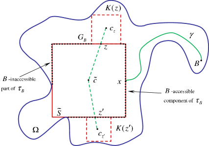
Figure 9: “$B$-accessible” and “$B$-inaccessible” subsets of ${\mathcal{T}}_{B}$.

The next definition enables us to specify the position of the $B$-accessible component ${\mathcal{T}}_{B,z}$ with respect to the interval $\partial\widetilde{S}\cap K(z)^{\operatorname{\,cl}}$.

Definition 2.17

By ${\mathcal{T}}_{B}^{\oplus}$ we denote a set consisting of all points $z\in{\mathcal{T}}_{B}$ such that

$$x\prec y~{}~{}\text{for every}~{}~{}x\in{\mathcal{T}}_{B}\cap K(z)^{\operatorname{\,cl}}~{}~{}\text{and every}~{}~{}y\in{\mathcal{T}}_{B,z}.$$

Correspondingly, ${\mathcal{T}}_{B}^{\ominus}$ is a subset of ${\mathcal{T}}_{B}$ consisting of all points $z$ such that

$$y\prec x~{}~{}\text{for every}~{}~{}x\in{\mathcal{T}}_{B}\cap K(z)^{\operatorname{\,cl}}~{}~{}\text{and every}~{}~{}y\in{\mathcal{T}}_{B,z}.$$

In particular, the point $z$ on Figure 9 belongs to ${\mathcal{T}}_{B}^{\oplus}$ while the point $z^{\prime}$ on this picture belongs ${\mathcal{T}}_{B}^{\ominus}$. Note that, by Lemma 2.14,

$${\mathcal{T}}_{B}^{\oplus}\cap{\mathcal{T}}_{B}^{\ominus}=\emptyset.$$ (2.34)

In turn, by Assumption 2.15,

$${\mathcal{T}}_{B}^{\oplus}\cup{\mathcal{T}}_{B}^{\ominus}={\mathcal{T}}_{B}$$ (2.35)

so that ${\mathcal{T}}_{B}^{\oplus}$ and ${\mathcal{T}}_{B}^{\ominus}$ is a partition of ${\mathcal{T}}_{B}$.

Our goal at this step of the proof is to show that representation (2.35) leads to a contradiction. Our proof of this fact relies on the following two lemmas which state that ${\mathcal{T}}_{B}^{\oplus}$ and ${\mathcal{T}}_{B}^{\ominus}$ are open subsets of ${\mathcal{T}}_{B}$, and, under Assumption 2.15, these sets are non-empty.

Lemma 2.18

The sets ${\mathcal{T}}_{B}^{\oplus}$ and ${\mathcal{T}}_{B}^{\ominus}$ are open subsets of ${\mathcal{T}}_{B}$ in the topology induced by the Euclidean metric on ${\mathcal{T}}_{B}$. In other words, for each $z\in{\mathcal{T}}_{B}^{\oplus}$ there exists $\varepsilon>0$ such that every point $y\in{\mathcal{T}}_{B}$, $\|y-z\|<\varepsilon$, belongs to ${\mathcal{T}}_{B}^{\oplus}$ (and the same statement is true for ${\mathcal{T}}_{B}^{\ominus}$).

Proof. Let $z\in{\mathcal{T}}_{B}^{\oplus}$. As we have noted above, the set ${\mathcal{T}}_{B,z}$ of all $B$-accessible points is non-empty so that there exists a point $z_{1}\in{\mathcal{T}}_{B,z}$. Recall that $z_{1}\in{\mathcal{T}}_{B}\setminus K(z)^{\operatorname{\,cl}}$. By Definition 2.16, there exists a path $\gamma_{1}$ which connects $z_{1}$ to $B$ in $\Omega$ such that $\gamma_{1}\setminus{z_{1}}\subset G_{B}\setminus K(z)^{\operatorname{\,cl}}$. Furthermore, since $z\in{\mathcal{T}}_{B}^{\oplus}$, we have

$$x\prec z_{1}~{}~{}\text{for every}~{}~{}x\in{\mathcal{T}}_{B}\cap K(z)^{\operatorname{\,cl}}.$$

Let $\varepsilon_{1}:=\operatorname{dist}(K(z)^{\operatorname{\,cl}},\gamma_{1})$. Since $\gamma_{1}\setminus{z_{1}}\subset G_{B}\setminus K(z)^{\operatorname{\,cl}}$, the path $\gamma_{1}$ and $K(z)^{\operatorname{\,cl}}$ have no common points, so that $\varepsilon_{1}>0$. Since $z_{1}\in\gamma_{1}$, we have $z_{1}\notin[K(z)]_{\varepsilon_{1}}$ so that

$$p\prec z_{1}~{}~{}\text{for every}~{}~{}p\in{\mathcal{T}}_{B}\cap[K(z)]_{\varepsilon_{1}}.$$ (2.36)

By Lemma 2.13, there exists $\delta>0$ such that for every $y\in{\mathcal{T}}_{B}$, $\|y-z\|<\delta$, we have $K(y)\subset[K(z)]_{\varepsilon_{1}}$. Hence,

$$K(y)\cap\gamma_{1}=\emptyset~{}~{}~{}\text{for every}~{}~{}~{}y\in{\mathcal{T}}_{B},~{}\|y-z\|<\delta.$$

See Figure 10.

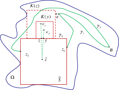
Figure 10: The path $\gamma_{1}$ joins $z_{1}$ to $B$ in $G_{B}\setminus K(z)^{\operatorname{\,cl}}$.

Prove that

$$y\in{\mathcal{T}}_{B}^{\oplus}~{}~{}~{}\text{for every}~{}~{}~{}y\in{\mathcal{T}}_{B},~{}\|y-z\|<\delta.$$

Suppose that there exists $y\in{\mathcal{T}}_{B}$ such that $\|y-z\|<\delta$ but $y\notin{\mathcal{T}}_{B}^{\oplus}$. Since the square $K(Y)\subset[K(z)]_{\varepsilon_{1}}$, by (2.36),

$$p\prec z_{1}~{}~{}\text{for every}~{}~{}p\in{\mathcal{T}}_{B}\cap K(y)^{\operatorname{\,cl}}.$$

By (2.34) and (2.35), $y\in{\mathcal{T}}_{B}^{\ominus}$ so that there exists a point $z_{2}\in{\mathcal{T}}_{B}\setminus K(y)^{\operatorname{\,cl}}$ such that

$$z_{2}\prec x~{}~{}\text{for every}~{}~{}x\in{\mathcal{T}}_{B}\cap K(y)^{\operatorname{\,cl}}.$$

Furthermore, there exists a path $\gamma_{2}$ joining $z_{2}$ to $B$ in $\Omega$ such that $\gamma_{2}\setminus\{z_{2}\}\subset G_{B}\setminus K(y)^{\operatorname{\,cl}}$. See Figure 10.

Thus the point $B$ can be joined by paths $\gamma_{i}$ in $\Omega$ to the points $z_{i},i=1,2$ which belong to distinct connected components of ${\mathcal{T}}_{B}\setminus K(y)^{\operatorname{\,cl}}$. These paths have the following property: $\gamma_{i}\setminus\{z_{i}\}\subset G_{B}\setminus K(y)^{\operatorname{\,cl}}$, $i=1,2$. Furthermore, the square $K=K(y)$ satisfies conditions (2.28) of Lemma 2.14.

However, by this lemma, $B$ can be joined to at most one connected component of the set ${\mathcal{T}}_{B}\setminus K(y)^{\operatorname{\,cl}}$ by a path of such a kind, a contradiction. This contradiction proves that each point $y\in{\mathcal{T}}_{B}$ in the $\delta$-neighborhood of $z$ belongs to ${\mathcal{T}}_{B}^{\oplus}$.

In the same way we prove a similar statement for the set ${\mathcal{T}}_{B}^{\ominus}$.

The lemma is completely proved.         $\Box$

Lemma 2.19

Under Assumption 2.15 both ${\mathcal{T}}_{B}^{\oplus}$ and ${\mathcal{T}}_{B}^{\ominus}$ are non-empty subsets of ${\mathcal{T}}_{B}$.

Proof. Let us prove that ${\mathcal{T}}_{B}^{\ominus}\neq\emptyset$.

Suppose that ${\mathcal{T}}_{B}^{\ominus}=\emptyset$. Since ${\mathcal{T}}_{B}^{\oplus}$ and ${\mathcal{T}}_{B}^{\ominus}$ are a partition of ${\mathcal{T}}_{B}$, we conclude that ${\mathcal{T}}_{B}={\mathcal{T}}_{B}^{\oplus}$. This equality implies the following

Statement B. For every $z\in{\mathcal{T}}_{B}$ there exists a point $y\in{\mathcal{T}}_{B}\setminus K(z)^{\operatorname{\,cl}}$ such that:

(i). $x\prec y$ for every $x\in{\mathcal{T}}_{B}\setminus K(z)^{\operatorname{\,cl}}$;

(ii). there exists a path $\gamma_{y}$ connecting $y$ to $B$ in $\Omega$ such that $\gamma_{y}\setminus\{y\}\subset G_{B}\setminus K(z)^{\operatorname{\,cl}}$.

See Figure 11.

Figure 11: The path $\gamma_{y}$ connects $y$ to $B$ in $G_{B}\setminus K(z)^{\operatorname{\,cl}}$.

Prove that Statement B leads to a contradiction whenever $z$ tends to the point $e_{{\mathcal{T}}_{B}}$ along ${\mathcal{T}}_{B}$. As in Lemma 2.12, without loss of generality we may assume that $\tilde{c}=(0,-R)$ where $R$ is the “radius” of $\widetilde{S}$. Furthermore, $z\in[a,b)$ and $e_{{\mathcal{T}}_{B}}\in(a,b]$ where $a=(-R,0)$ and $b=(R,0)$. Thus $[a,b]$ is a side of $\widetilde{S}$ lying on the real axes.

Let $z=(z_{1},0)$ and $e_{{\mathcal{T}}_{B}}=(h,0)$ where $-R\leq z_{1}<h$ and $-R<h\leq R$.

We use the same notation as in Lemma 2.12. In particular, as in formulas (2.13) and (2.14),

$$K(z)^{\operatorname{\,cl}}\cap Ox=[a_{z},b_{z}]$$ (2.37)

where

$$a_{z}=z_{1}\left(1+\tfrac{r_{z}}{R}\right)-r_{z}~{}~{}~{}\text{and}~{}~{}~{}b_{z}=z_{1}\left(1+\tfrac{r_{z}}{R}\right)+r_{z}.$$

See Figure 12.

Figure 12:  

Let $z\in{\mathcal{T}}_{B}$ and $z\to e_{{\mathcal{T}}_{B}}$, i.e, $z_{1}\to h$. Consider two cases.

The first case. Let us assume that

$$\limsup_{z\to e_{{\mathcal{T}}_{B}},\,z\in{\mathcal{T}}_{B}}r_{z}=L>0.$$ (2.38)

Prove that in this case there exists $\bar{z}=(\bar{z}_{1},0)\in[a_{z},e_{{\mathcal{T}}_{B}})$ such that

$$e_{{\mathcal{T}}_{B}}\in[a_{\bar{z}},b_{\bar{z}}].$$ (2.39)

Note that, since $a_{\bar{z}}\leq\bar{z}_{1}<h$, property (2.39) is equivalent to the inequality $h\leq b_{\bar{z}}$.

Simple calculations show that if

$$r_{\bar{z}}\geq L/2~{}~{}~{}\text{and}~{}~{}~{}\|\bar{z}-e_{{\mathcal{T}}_{B}}\|\leq\tfrac{1}{4}\min\{1,L/R\}\,\|e_{{\mathcal{T}}_{B}}-a\|,$$ (2.40)

then (2.39) holds. In fact, since $r_{\bar{z}}\geq L/2$, we obtain

$$r_{\bar{z}}\left(1+\tfrac{\bar{z}_{1}}{R}\right)\geq\tfrac{L}{2}\left(1+\tfrac{\bar{z}_{1}}{R}\right)=\tfrac{L}{2R}\,\|\bar{z}-a\|.$$

Furthermore, by (2.40),

$$\|\bar{z}-a\|\geq\|e_{{\mathcal{T}}_{B}}-a\|-\|\bar{z}-e_{{\mathcal{T}}_{B}}\|\geq\|e_{{\mathcal{T}}_{B}}-a\|-\tfrac{1}{4}\|e_{{\mathcal{T}}_{B}}-a\|=\tfrac{3}{4}\|e_{{\mathcal{T}}_{B}}-a\|$$

proving that

$$r_{\bar{z}}\left(1+\tfrac{\bar{z}_{1}}{R}\right)\geq\tfrac{3L}{8R}\,\|e_{{\mathcal{T}}_{B}}-a\|.$$

Hence, by (2.40),

$$r_{\bar{z}}\left(1+\tfrac{\bar{z}_{1}}{R}\right)\geq\|\bar{z}-e_{{\mathcal{T}}_{B}}\|=h-\bar{z}_{1}$$

so that

$$b_{\bar{z}}=\bar{z}_{1}\left(1+\tfrac{r_{\bar{z}}}{R}\right)+r_{\bar{z}}\geq h$$

proving (2.39).

Of course, condition (2.38) guarantees the existence of a point $\bar{z}\in{\mathcal{T}}_{B}$ satisfying requirements (2.40).

Combining (2.39) with (2.37) we conclude that $K(\bar{z})^{\operatorname{\,cl}}\ni e_{{\mathcal{T}}_{B}}$ so that the point $y$ satisfying conditions of part (i) of Statement B does not exist. This contradiction shows that equality (2.38) does not hold.

The second case.

$$\lim_{z\to e_{{\mathcal{T}}_{B}},\,z\in{\mathcal{T}}_{B}}r_{z}=0.$$ (2.41)

Let $\widetilde{z}=(\widetilde{z}_{1},0)$, $-R\leq\widetilde{z}_{1}<h$, and let

$$K(\widetilde{z})^{\operatorname{\,cl}}\cap Ox=[a_{\widetilde{z}},b_{\widetilde{z}}]$$

By Statement B, there exist a point $y=(y_{1},0),$ $b_{\widetilde{z}}<y_{1}<h,$ and a path $\gamma_{y}$ which joins $y$ to $B$ in $\Omega$ such that $\gamma_{y}\setminus\{y\}\subset G_{B}\setminus K(y)^{\operatorname{\,cl}}$. See Figure 12.

Let $\varepsilon:=\operatorname{dist}(\gamma_{y},\partial\Omega)$. Since $\gamma_{y}$ is a compact subset of $\Omega$, the number $\varepsilon$ is positive. Note that the point $e_{{\mathcal{T}}_{B}}=(h,0)\in\partial\Omega$ so that

$$\operatorname{dist}(\gamma_{y},e_{{\mathcal{T}}_{B}})\geq\varepsilon.$$ (2.42)

By (2.41), there exist $\delta\in(0,\varepsilon/4)$ such that

$$r_{z}<\varepsilon/8~{}~{}\text{for every}~{}~{}~{}z\in{\mathcal{T}}_{B},\|z-e_{{\mathcal{T}}_{B}}\|<\delta.$$

See Figure 12.

Fix such a point $z=(z_{1},0)$ satisfying these conditions. Then

$$\operatorname{dist}(K(z),e_{{\mathcal{T}}_{B}})\leq\|z-e_{{\mathcal{T}}_{B}}\|+\|z-c_{z}\|+r_{z}<\delta+2r_{z}<\delta+\varepsilon/4<\varepsilon/2$$

so that, by (2.42),

$$\gamma_{y}\cap K(z)^{\operatorname{\,cl}}=\emptyset.$$

On the other hand, by part (ii) of Statement B, there exists a point $x=(x_{1},0)$ such that

(a). $z^{\prime}\prec x$ for all $z^{\prime}\in K(z)^{\operatorname{\,cl}}\cap{\mathcal{T}}_{B}$;

(b). there exists a path$\gamma_{x}$ connecting $x$ to $B$ in $\Omega$ such that $\gamma_{x}\setminus\{x\}\subset G_{B}\setminus K(z)^{\operatorname{\,cl}}$.

Thus both connected components of ${\mathcal{T}}_{B}\setminus K(z)^{\operatorname{\,cl}}$ are $B$-accessible which contradicts Lemma 2.14. This contradiction shows that Statement B is wrong in both cases proving that ${\mathcal{T}}_{B}^{\ominus}\neq\emptyset$.

In the same way we show that the points of ${\mathcal{T}}_{B}$ which are close enough to the point $b_{{\mathcal{T}}_{B}}$ belong to ${\mathcal{T}}_{B}^{\oplus}$ proving that ${\mathcal{T}}_{B}^{\oplus}\neq\emptyset$.

The proof of the lemma is complete.         $\Box$

We are in a position to finish the proof of Theorem 2.6.

Proof of Theorem 2.6. Under Assumption 2.15 the sets ${\mathcal{T}}_{B}^{\oplus}$ and ${\mathcal{T}}_{B}^{\ominus}$ are a partition of ${\mathcal{T}}_{B}$. Clearly, ${\mathcal{T}}_{B}$ is a connected topological space in induced Euclidean topology. But ${\mathcal{T}}_{B}^{\oplus}$ and ${\mathcal{T}}_{B}^{\ominus}$ are non-empty and open subsets of ${\mathcal{T}}_{B}$ in this topology, see Lemma 2.18 and Lemma 2.19. This contradicts the connectedness of ${\mathcal{T}}_{B}$.

Thus Assumption 2.15 is not true which easily implies the statement of Theorem 2.6. In fact, if there exists $z\in{\mathcal{T}}_{B}$ such that $B\in K(z)$, then we put $Q:=K(z)$. Since $z\in K(z)^{\operatorname{\,cl}}\cap\widetilde{S}^{\operatorname{\,cl}}\cap\Omega$, see (2.12), condition (i) of the theorem is satisfied. Furthermore, the first option of part (ii) of this theorem (i.e., the requirement $B\in K(z)$) holds, and the proof in this case is complete.

Suppose that $B\notin K(z)$ for every $z\in{\mathcal{T}}_{B}$. Since Assumption 2.15 is not true, there exists $z\in{\mathcal{T}}_{B}$ such that part (ii) of Assumption 2.15 does not hold. This means that

$$\forall z^{\prime}\in{\mathcal{T}}_{B},\forall~{}\text{path}~{}\gamma~{}\text{joining}~{}z^{\prime}~{}\text{to}~{}B,~{}\gamma\setminus\{z^{\prime}\}\subset G_{B},~{}\text{we have}~{}\gamma\cap K(z)^{\operatorname{\,cl}}\neq\emptyset.$$ (2.43)

We again put $Q:=K(z)$. Since part (i) of Theorem 2.6 is satisfied and, by the assumption, $B\notin Q=K(z)$, it remains to prove the statement (2.4). This statement is equivalent to the following:

$$\text{For every}~{}a\in\widetilde{S}~{}\text{and every path}~{}\gamma~{}\text{joining}~{}a~{}\text{to}~{}B~{}\text{in}~{}\Omega~{}\text{we have}~{}\gamma\cap K(z)^{\operatorname{\,cl}}\neq\emptyset.$$ (2.44)

Prove this fact by representing $\gamma$ in a parametric form, i.e., as a graph of a continuous mapping $\Gamma:[0,1]\to\Omega$ such that $\Gamma(0)=a$ and $\Gamma(1)=B$. Let $a^{\prime}:=\Gamma(t_{\max})$ where

$$t_{\max}:=\max\{t\in[0,1]:\gamma(t)\in\partial\widetilde{S}\}.$$

Since $a\in\widetilde{S}$ and $B\notin\widetilde{S}^{\operatorname{\,cl}}$, the point $a^{\prime}$ is well defined. By $\gamma^{\prime}$ we denote the arc of $\gamma$ from $a^{\prime}$ to $B$. By definition of $t_{\max}$,

$$\gamma^{\prime}\setminus\{a^{\prime}\}\cap\widetilde{S}^{\operatorname{\,cl}}=\emptyset,$$ (2.45)

so that, by Lemma 2.8 and Definition 2.9, $a^{\prime}\in{\mathcal{T}}_{B}$ and $\gamma^{\prime}\setminus\{a^{\prime}\}\subset G_{B}$. Then, by (2.43), $\gamma^{\prime}\cap K(z)^{\operatorname{\,cl}}\neq\emptyset$ proving (2.44).

The proof of “The Square Separation Theorem” 2.6 is complete.         $\Box$

Remark 2.20

Note that we are able to prove the following slight improvement of the statement (2.44):

$$\forall~{}a\in\widetilde{S}^{\operatorname{\,cl}}\cap\Omega~{}\text{and}~{}\forall~{}\text{path}~{}\gamma~{}\text{joining}~{}a~{}\text{to}~{}B~{}\text{in}~{}\Omega~{}\text{we have}~{}\gamma\cap K(z)^{\operatorname{\,cl}}\neq\emptyset.$$ (2.46)

In fact, let $a\in\partial\widetilde{S}\cap\Omega$. If $\gamma\cap\widetilde{S}\neq\emptyset$, then the proof of (2.46) is reduced to the previous case of $a\in\widetilde{S}$ proven below. If $\gamma\cap\widetilde{S}=\emptyset$, then we can put $a^{\prime}=a$ in (2.45) so that this equality will be satisfied.

This enables us to modify the statement (2.4) of Theorem 2.6 as follows:

$$\widetilde{S}^{\operatorname{\,cl}}\cap\Omega~{}~{}\text{and}~{}~{}B~{}~{}\text{lie in different connected components of}~{}~{}\Omega\setminus Q^{\operatorname{\,cl}}.\hskip 28.45274pt\vartriangleleft$$

We finish the section with two remarks which present certain additional useful properties of the square $Q$ from formulation of Theorem 2.6.

Remark 2.21

We notice that the square $Q$ from Theorem 2.6 coincides with a square $K(z)$ for some $z\in{\mathcal{T}}_{B}$. Applying part (d) and part (e) of Lemma 2.11 to $K(z)=Q$ we conclude that $Q$ has the following properties:

(i). The line segment $[\tilde{c},c_{Q}]\subset\Omega$;

(ii). For every point $u\in Q^{\operatorname{\,cl}}\cap\Omega$ there exists a path $\gamma$ which joins $u$ to $B$ in $\Omega$ such that $(\gamma\setminus\{u\})\cap\widetilde{S}^{\operatorname{\,cl}}=\emptyset$.         $\vartriangleleft$

Our next remark relates to a certain improvement of part (ii) of “The Square Separation Theorem” 2.6, see Remark 2.23 below. This improvement is based on the following

Lemma 2.22

Let $K$ be a square and let $x,y\in\Omega\setminus K^{\operatorname{\,cl}}$. Suppose there exists a polygonal path $\gamma$ which joins $x$ to $y$ in $\Omega$ such that $\gamma\cap K=\emptyset$.

Then there exists a polygonal path $\widetilde{\gamma}$ joining $x$ to $y$ in $\Omega$ such that $\widetilde{\gamma}\cap K^{\operatorname{\,cl}}=\emptyset$.

Proof. We will obtain the path $\widetilde{\gamma}$ by a slight modification of $\gamma$ around the set $H:=\gamma\cap\,\partial K$. Since $\gamma$ is a polygonal path in $\Omega$, the set $H$ can be represented as a union of a finite number of pairwise disjoint subarcs of $\gamma$ lying on $\partial K$. In other words,

$$H=\gamma\cap K^{\operatorname{\,cl}}=\bigcup_{i=1}^{m}\gamma_{i}$$

where each $\gamma_{i}$ is either a subarc of $\gamma$ or a point of $\gamma$, and $\gamma_{i}\cap\gamma_{j}=\emptyset$, $1\leq i,j\leq m,$ $i\neq j$.

Let us represent $\gamma$ as a graph of a continuous mapping $\Gamma:[0,1]\to\Omega$ such that $\Gamma(0)=x$ and $\Gamma(1)=y$. Then each $\gamma_{i}$ is the graph of the mapping $\Gamma:[a_{i},b_{i}]\to\Omega$ where

$$0\leq a_{i}\leq b_{i}\leq 1.$$

Since the arcs $\gamma_{i}$ are disjoint, the line segments $[a_{i},b_{i}],i=1,...,m,$ are disjoint as well.

Let $A_{i}:=\Gamma(a_{i})$ and $B_{i}:=\Gamma(b_{i})$ be the beginning and the end of the arc $\gamma_{i}$ respectively. Let

$$\varepsilon:=\min_{1\leq i,j\leq m,\,i\neq j}\{\operatorname{dist}(\gamma,\partial\Omega),\operatorname{dist}(\gamma_{i},\gamma_{j})\}.$$

Then $[\gamma_{i}]_{\varepsilon}\subset\Omega$, $1\leq i\leq m,$ and

$$[\gamma_{i}]_{\varepsilon}\cap[\gamma_{j}]_{\varepsilon}=\emptyset,~{}~{}~{}i,j=1,...,m,~{}~{}i\neq j.$$

(Recall that $[\,\cdot\,]_{\varepsilon}$ denotes the $\varepsilon$-neighborhood of a set.) Clearly, the set

$$T_{i}:=[\gamma_{i}]_{\varepsilon}\setminus K^{\operatorname{\,cl}}$$

is a connected open subset of $\Omega$.

Let $\gamma_{i}^{(p)}$ be the arc of $\gamma$ joining $x$ to $A_{i}$, and let $\gamma_{i}^{(f)}$ be the arc of $\gamma$ joining $B_{i}$ to $y$. Since $\gamma$ is a continuous curve and $x,y\notin K^{\operatorname{\,cl}}$, there are exist points $\widetilde{A}_{i}\in\gamma_{i}^{(p)}\cap T_{i}$ and $\widetilde{B}_{i}\in\gamma_{i}^{(f)}\cap T_{i}$. Since $T_{i}$ is a connected subset of $\Omega$, there exists a polygonal path $\widetilde{\gamma}_{i}$ joining $\widetilde{A}_{i}$ to $\widetilde{B}_{i}$ in $T_{i}$.

Now we replace the arc $\gamma_{i}$ by $\widetilde{\gamma}_{i}$ for each $i\in\{1,...,m\}$. As a result we obtain a new polygonal path $\widetilde{\gamma}$ which connects $x$ to $y$ in $\Omega$ and has no common points with $K^{\operatorname{\,cl}}$.         $\Box$

Remark 2.23

Lemma 2.22 and Remark 2.20 enable us to make further improvement of part (ii) of “The Square Separation Theorem” 2.6:

(ii^′). Either $B\in Q^{\operatorname{\,cl}}$ or

$$\widetilde{S}^{\operatorname{\,cl}}\cap\Omega~{}~{}\text{and}~{}~{}B~{}~{}\text{lie in different connected components of}~{}~{}\Omega\setminus Q.$$ (2.47)

Thus $\gamma\cap Q\neq\emptyset$ for every $z\in\widetilde{S}^{\operatorname{\,cl}}\cap\Omega$ and every path $\gamma$ which joins $z$ to $B$ in $\Omega$.          $\vartriangleleft$

3. Proof of “The Wide Path Theorem”

Basing on “The Square Separation Theorem” 2.6 given $\bar{x},\bar{y}\in\Omega$ we construct “The Wide Path” ${\cal WP}_{\Omega}^{(\bar{x},\bar{y})}$, see Theorem 1.9, as follows.

Let

$$S_{1}:=S(\bar{x},\operatorname{dist}(\bar{x},\partial\Omega)).$$

Thus $S_{1}$ is the maximal (with respect to inclusion) square in $\Omega$ centered at $\bar{x}$. If $\bar{y}\in S_{1}^{\operatorname{\,cl}}$, then we put $k=1$ and stop. If $\bar{y}\in\Omega\setminus S_{1}^{\operatorname{\,cl}}$, we apply Theorem 2.6 to $\widetilde{S}:=S_{1}$ and $B:=\bar{y}$. By this theorem, there exist a square $S_{2}\subset\Omega\setminus S_{1}^{\operatorname{\,cl}}$ such that

$$S_{1}^{\operatorname{\,cl}}\cap S_{2}^{\operatorname{\,cl}}\cap\Omega\neq\emptyset,$$

and either $\bar{y}\in S_{2}^{\operatorname{\,cl}}$ or

$${S_{2}~{}~{}\text{\it{and}}~{}~{}\bar{y}~{}~{}\text{{\it lie in distinct connected components of}}~{}~{}\Omega\setminus S_{2}^{\operatorname{\,cl}}.}$$

If $\bar{y}\in S_{2}^{\operatorname{\,cl}}$, then we put $k=2$ and stop. If not, using “The Square Separation Theorem” we construct a square $S_{3}$, etc.

Continuing this procedure we obtain a sequence $\{S_{1},S_{2},...,S_{m},...\}$ of squares (finite or infinite). Let $k$ be the number of its elements; thus $k=\infty$ whenever the sequence is infinite.

In the next lemma we present main properties of the squares $S_{i},i=1,2,...$. Let $c_{i}$ and $r_{i}$ be the center and “radius” of the square $S_{i}$ respectively, i.e.,

$$S_{i}=S(c_{i},r_{i}),~{}~{}~{}i=1,2,...~{}.$$

Lemma 3.1

(a). $\bar{x}\in S_{1}$ and $\bar{y}\in S_{k}^{\operatorname{\,cl}}$ provided $k<\infty$. Furthermore, if $1<k<\infty$, then $\operatorname{dist}(\bar{y},S_{k-1})=\operatorname{diam}S_{k}$ ;

(b). $S_{i}\subset\Omega$ and $S_{i}^{\operatorname{\,cl}}\cap\partial\Omega\neq\emptyset$ for every $1\leq i<k$ ;

(c). For all $i,1\leq i<k$, we have $S_{i}^{\operatorname{\,cl}}\cap S_{i+1}=\emptyset$, but $S_{i}^{\operatorname{\,cl}}\cap S_{i+1}^{\operatorname{\,cl}}\cap\Omega\neq\emptyset$.

Furthermore,

$$[c_{i},c_{i+1}]\subset\Omega,~{}~{}~{}1\leq i<k\,;$$ (3.1)

(d). Let $1\leq i<k-1$ and let $a\in S_{i}^{\operatorname{\,cl}}\cap\Omega$. Then $\gamma\cap S_{i+1}\neq\emptyset$ for any path $\gamma$ connecting $a$ to $\bar{y}$ in $\Omega$ ;

(e). For every $1\leq i<k$ and every $z\in S_{i+1}^{\operatorname{\,cl}}\cap\Omega$ there exists a path $\gamma$ joining $z$ to $\bar{y}$ in $\Omega$ such that $(\gamma\setminus\{z\})\cap S_{i}^{\operatorname{\,cl}}=\emptyset$.

Proof. Parts (a) and (b) follow from the construction of the squares $\{S_{i}\}$ and the proof of “The Square Separation Theorem” 2.6; see part (b) of Lemma 2.11. Since the unique requirement to the square $S_{k}$ is that $S_{k}\ni\bar{y}$ and $S_{k}$ touches $S_{k-1}$, one can choose $S_{k}$ in such a way that $\operatorname{dist}(\bar{y},S_{k-1})=\operatorname{diam}S_{k}$.

Note that part (c) of the lemma directly follows from the construction of the squares $\{S_{i}\}$, part (i) of Theorem 2.6 and (2.11). In turn, part (d) and part (e) are consequences of (2.47), see Remark 2.23, and part (ii) of Remark 2.21 respectively.         $\Box$

In the next four lemmas we present additional properties of the squares $\{S_{1},S_{2},...\}$ which we need for the proofs of Theorems 1.9 and 1.10.

Lemma 3.2

(i). Let $k>1$ and let $1\leq i<k-1$. Let $a\in S_{i}^{\operatorname{\,cl}}\cap\Omega$ and let $\gamma$ be a path joining $a$ to $\bar{y}$ in $\Omega$. Then $\gamma\cap S_{j}\neq\emptyset$ for every $j,i<j<k$;

(ii). $S_{i}^{\operatorname{\,cl}}\cap S_{j}=\emptyset$ for all $i,j\geq 1$, $i\neq j$.

Proof. (i). See Figure 13 for an example of a path $\gamma$ joining in $\Omega$ a point $a\in S_{2}^{\operatorname{\,cl}}\cap\Omega$ to $\bar{y}$.

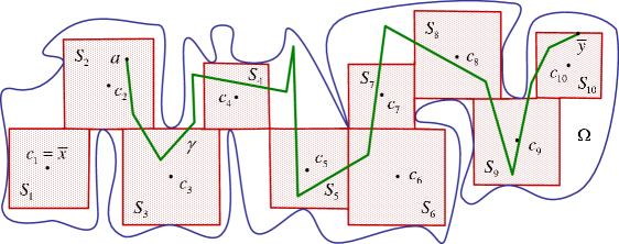
Figure 13: A path $\gamma$ connects a point $a\in S_{2}$ to $\bar{y}$ in $\Omega$.

We prove property (i) by induction on $j$. For $j=i+1$ it follows from part (d) of Lemma 3.1. Suppose that $\gamma\cap S_{j}\neq\emptyset$ for some $j>i+1$. Prove that $\gamma\cap S_{j+1}\neq\emptyset$ as well.

In fact, let $b\in\gamma\cap S_{j}$ and let $\gamma_{b}$ be the arc of $\gamma$ from $b$ to $\bar{y}$. Since $b\in S_{j}^{\operatorname{\,cl}}\cap\Omega$, by property (d) of Lemma 3.1, $\gamma_{b}\cap S_{j+1}\neq\emptyset$, proving the statement (i) of the lemma.

(ii). Let $i<j$. Prove this statement by induction on $j$. By part (c) of Lemma 3.1, $S_{i}^{\operatorname{\,cl}}\cap S_{i+1}=\emptyset$.

Suppose that $S_{i}^{\operatorname{\,cl}}\cap S_{j}=\emptyset$ for some $j>i+1$, and prove that $S_{i}^{\operatorname{\,cl}}\cap S_{j+1}=\emptyset$ as well. Assume that it is not true, i.e., that there exists $z\in S_{i}^{\operatorname{\,cl}}\cap S_{j+1}$. Since $z\in S_{j+1}$, by part (e) of Lemma 3.1, there exists a path $\gamma_{1}$ joining $z$ to $\bar{y}$ in $\Omega$ such that $\gamma_{1}\cap S_{j}^{\operatorname{\,cl}}=\emptyset.$

On the other hand, $z\in S_{i}^{\operatorname{\,cl}}\cap S_{j+1}\subset S_{i}^{\operatorname{\,cl}}\cap\Omega$ so that, by part (i) of the present lemma, $\gamma_{1}\cap S_{j}^{\operatorname{\,cl}}\neq\emptyset$, a contradiction which proves part (ii) for $i<j$.

Let $j<i$. As we have proved, in this case $S_{j}^{\operatorname{\,cl}}\cap S_{i}=\emptyset$ so that $S_{j}\cap S_{i}=\emptyset$ as well. Hence $S_{i}^{\operatorname{\,cl}}\cap S_{j}=\emptyset$, and the proof of the lemma is complete.         $\Box$

Lemma 3.3

$k<\infty$, i.e., $\{S_{1},S_{2},...\}$ is a finite family of squares.

Proof. Let $\gamma$ be a path connecting $\bar{x}$ to $\bar{y}$ in $\Omega$. Since $\bar{x}=c_{S_{1}}\in S_{1}$, by part (i) of Lemma 3.2, $\gamma\cap S_{i}\neq\emptyset$ for every $1\leq i<k$.

Note that the path $\gamma$ is a compact subset of $\Omega$ so that $\varepsilon:=\operatorname{dist}(\gamma,\partial\Omega)>0$. Prove that for each square $S_{i}$, $i\geq 1$, we have $\operatorname{diam}S_{i}\geq\varepsilon$.

In fact, let $a\in\gamma\cap S_{i}$. Then $\operatorname{dist}(a,\partial\Omega)\geq\operatorname{dist}(\gamma,\partial\Omega)=\varepsilon$.

Recall that $S_{i}=S(c_{i},r_{i})$, $i=1,2,...\,$. By part (b) of Lemma 3.1, $S_{i}\subset\Omega$ and $S_{i}^{\operatorname{\,cl}}\cap\partial\Omega\neq\emptyset$, so that $r_{i}=\operatorname{dist}(c_{i},\partial\Omega)$. Hence,

$$\varepsilon\leq\operatorname{dist}(a,\partial\Omega)\leq\|a-c_{i}\|+\operatorname{dist}(c_{i},\partial\Omega)\leq r_{i}+r_{i}=\operatorname{diam}S_{i}.$$

By part (ii) of Lemma 3.2, the squares of the family ${\mathcal{S}}=\{S_{i}:1\leq i<k\}$ are non-overlapping. Since the diameter of each square from ${\mathcal{S}}$ is at least $\varepsilon$, the domain $\Omega$ contains at most $|\Omega|/\varepsilon^{2}$ squares from this family. Since $\Omega$ is bounded, this number is finite, and the proof is complete.         $\Box$

The next lemma provides a certain improvement of Lemma 3.2.

Lemma 3.4

(i). Let $k>1$ and let  $1\leq i<m-1\leq k-1$. Let $a\in S_{i}^{\operatorname{\,cl}}\cap\Omega$, $b\in S_{m}^{\operatorname{\,cl}}\cap\Omega$, and let $\gamma$ be a path joining $a$ to $b$ in $\Omega$. Then $\gamma\cap S_{j}\neq\emptyset$ for every $j,\,i<j<m$;

(ii). $S_{i}^{\operatorname{\,cl}}\cap S_{j}^{\operatorname{\,cl}}\cap\Omega=\emptyset$ for every $1\leq i,j\leq k$ such that $|i-j|>1$;

(iii). Let $1\leq i\leq m\leq k$ and let $a\in S_{i}^{\operatorname{\,cl}}\cap\Omega$, $b\in S_{m}^{\operatorname{\,cl}}\cap\Omega$. There exists a simple path $\gamma$ which joins $a$ to $b$ in $\Omega$ such that

$$\gamma\subset\bigcup_{j=i}^{m}\,\left(S_{j}^{\operatorname{\,cl}}\,{\bigcap}\,\Omega\right).$$ (3.2)

Furthermore, $\gamma\cap S_{j}^{\operatorname{\,cl}}=\emptyset$ provided $j>m+1$ or $j<i-1$, and $(\gamma\setminus\{a\})\cap S_{i-1}^{\operatorname{\,cl}}=\emptyset$ and $(\gamma\setminus\{b\})\cap S_{m+1}^{\operatorname{\,cl}}=\emptyset$.

Proof. (i). We prove the statement (i) by induction on $n=m-j$, $1\leq n<m-i$. Let $n=1$, i.e., $j=m-1$. Prove that $\gamma\cap S_{m-1}\neq\emptyset$.

Since $b\in S_{m}^{\operatorname{\,cl}}\cap\Omega$, by property (e) of Lemma 3.1, there exists a path $\gamma_{1}$ joining $b$ to $\bar{y}$ in $\Omega$ such that

$$(\gamma_{1}\setminus\{b\})\cap S_{m-1}^{\operatorname{\,cl}}=\emptyset.$$ (3.3)

Let $\widetilde{\gamma}:=\gamma\cup\gamma_{1}$. Then $\widetilde{\gamma}$ is a path which connects $a$ to $\bar{y}$ in $\Omega$ so that, by part (i) of Lemma 3.2, $\widetilde{\gamma}\cap S_{m-1}\neq\emptyset$.

Recall that $b\in S_{m}^{\operatorname{\,cl}}$. Since $S_{m}^{\operatorname{\,cl}}\cap S_{m-1}\neq\emptyset$, see part (ii) of Lemma 3.2, $b\notin S_{m-1}$. Combining this with (3.3) we conclude that $\gamma_{1}\cap S_{m-1}=\emptyset$. Since

$$\widetilde{\gamma}\cap S_{m-1}=(\gamma\cup\gamma_{1})\cap S_{m-1}\neq\emptyset,$$

we obtain that $\gamma\cap S_{m-1}\neq\emptyset$.

Now given $j=m-n+1$ suppose that $\gamma\cap S_{j}\neq\emptyset$. Prove that $\gamma\cap S_{j-1}\neq\emptyset$ as well.

We follow the same scheme as for the case $j=m-1$. Let $\widetilde{b}\in\gamma\cap S_{j}$. Since $\widetilde{b}\in S_{j}\subset S_{j}^{\operatorname{\,cl}}\cap\Omega$, by part (e) of Lemma 3.1, there exists a path $\gamma^{\prime}$ which joins $\widetilde{b}$ to $\bar{y}$ in $\Omega$ such that

$$(\gamma^{\prime}\setminus\{\widetilde{b}\})\cap S_{j-1}^{\operatorname{\,cl}}=\emptyset.$$ (3.4)

Let $\gamma^{\prime\prime}$ be the arc of $\gamma$ from $a$ to $\widetilde{b}$. Then the path $\bar{\gamma}:=\gamma^{\prime}\cup\gamma^{\prime\prime}$ joins $a$ to $\bar{y}$ in $\Omega$ so that, by part (i) of Lemma 3.2, $\bar{\gamma}\cap S_{j-1}\neq\emptyset$.

Since $\widetilde{b}\in S_{j}$ and $S_{j}\cap S_{j-1}=\emptyset$, see part (ii) of Lemma 3.2, we conclude that $b\notin S_{j-1}$. This and (3.4) imply that $\gamma^{\prime}\cap S_{j-1}^{\operatorname{\,cl}}=\emptyset$. Since

$$\bar{\gamma}\cap S_{j-1}=(\gamma^{\prime}\cup\gamma^{\prime\prime})\neq\emptyset,$$

we conclude that $\gamma^{\prime\prime}\cap S_{j-1}^{\operatorname{\,cl}}\neq\emptyset$. But $\gamma^{\prime\prime}$ is a subarc of $\gamma$ so that $\gamma\cap S_{j-1}^{\operatorname{\,cl}}\neq\emptyset$ proving part (i) of the lemma.

(ii). Suppose that $S_{i}^{\operatorname{\,cl}}\cap S_{j}^{\operatorname{\,cl}}\cap\Omega\neq\emptyset$ for some $1\leq i<j\leq k$ such that $i+1<j$. Let $z\in S_{i}^{\operatorname{\,cl}}\cap S_{j}^{\operatorname{\,cl}}\cap\Omega$. Since $S_{i}\cap S_{j}=\emptyset$, the point $z\in\partial S_{i}\cap\partial S_{j}$.

Let $\gamma:=[c_{i},z]\cup[z,c_{j}]$. (Recall that $c_{i}$ is the center of $S_{i}$.) Clearly, $c_{i}\in S_{i}^{\operatorname{\,cl}}\cap\Omega$ and $c_{j}\in S_{j}^{\operatorname{\,cl}}\cap\Omega$ so that, by part (i) of the present lemma,

$$\gamma\cap S_{i+1}\neq\emptyset.$$ (3.5)

However $\gamma\setminus\{z\}\subset S_{i}\cup S_{j}$. Since $S_{i},S_{i+1}$ and $S_{j}$ are pairwise disjoint, $S_{i+1}\cap(S_{i}\cup S_{j})=\emptyset$, so that, by (3.5), $z\in S_{i+1}$. Since $z\in S_{i}^{\operatorname{\,cl}}$, this implies $S_{i}^{\operatorname{\,cl}}\cap S_{i+1}\neq\emptyset$ which contradicts part (ii) of Lemma 3.2.

(iii). Recall that $S_{j}=S(c_{j},r_{j})$. Let $\gamma_{1}:=[a,c_{i}]$ and let $\gamma_{3}:=[c_{m},b]$. (Whenever $a=c_{i}$ or $b=c_{m}$ we ignore $\gamma_{1}$ or $\gamma_{3}$ respectively.) By $\gamma_{2}$ we denote a polygonal path with vertices in $c_{i},c_{i+1},...,c_{m-1},c_{m}$. Then a path $\gamma:=\gamma_{1}\cup\gamma_{2}\cup\gamma_{3}$ connects $a$ to $b$.

Clearly, $\gamma_{1}=[a,c_{i}]\subset S_{i}^{\operatorname{\,cl}}\cap\Omega$ and $\gamma_{1}\setminus\{a\}\subset S_{i}$. Also $\gamma_{3}=[c_{m},b]\subset S_{m}^{\operatorname{\,cl}}\cap\Omega$ and $\gamma_{3}\setminus\{b\}\subset S_{m}$.

On the other hand, by property (3.1), see part (c) of Lemma 3.1,

$$[c_{j},c_{j+1}]\subset(S_{j}^{\operatorname{\,cl}}\cup S_{j+1}^{\operatorname{\,cl}})\cap\Omega$$

so that $\gamma_{2}\subset\cup\{S_{j}^{\operatorname{\,cl}}\cap\Omega:i\leq j\leq m\}$. These properties of the paths $\gamma_{i}$, $i=1,2,3,$ prove (3.2).

The second statement of part(iii) immediately follows from the fact that the squares $\{S_{j}\}$ are pairwise disjoint and $S_{j_{1}}^{\operatorname{\,cl}}\cap S_{j_{2}}^{\operatorname{\,cl}}\cap\Omega=\emptyset$ whenever $|j_{1}-j_{2}|>1$. See part (ii) of Lemma 3.2 and part (ii) of the present lemma.

The proof of the lemma is complete.         $\Box$

Lemma 3.5

Let $1<i<k$. Then the set $\cup\{S_{j}:i<j\leq k\}$ and the point $\bar{y}$ belong to the same connected component of  $\Omega\setminus S_{i}^{\operatorname{\,cl}}$.

In turn, the set  $\cup\{S_{j}:1\leq j<i\}$ and the point $\bar{x}$ belong to another connected component of  $\Omega\setminus S_{i}^{\operatorname{\,cl}}$.

Proof. Let $a\in\cup\{S_{j}:i<j\leq k\}$ so that $a\in S_{j}$ for some $i+1\leq j\leq k$. Since $\bar{y}\in S_{k}^{\operatorname{\,cl}}$, by part (iii) of Lemma 3.4, there exists a path $\gamma$ which connects $a$ to $\bar{y}$ in $\Omega$ such that $\gamma\setminus\{a\}\cap S_{i}^{\operatorname{\,cl}}=\emptyset$. But $S_{j}\cap S_{i}^{\operatorname{\,cl}}=\emptyset$, see part (ii) of Lemma 3.2, so that $\gamma\setminus\{a\}\cap S_{i}^{\operatorname{\,cl}}=\emptyset$. This proves that $a$ and $\bar{y}$ belong to the same connected component of $\Omega\setminus S_{i}^{\operatorname{\,cl}}$.

In the same way we show that every point

$$b\in\cup\{S_{j}:1\leq j<i\}$$

belong to the same connected component of $\Omega\setminus S_{i}^{\operatorname{\,cl}}$ as the point $\bar{x}$.

It remains to note that, by part(i) of Lemma 3.4, $\gamma\cap S_{i}^{\operatorname{\,cl}}\neq\emptyset$ for every path $\gamma$ joining $\bar{x}$ to $\bar{y}$ in $\Omega$ so that $\bar{x}$ and $\bar{y}$ belong to distinct connected components of $\Omega\setminus S_{i}^{\operatorname{\,cl}}$.

The proof of the lemma is complete.         $\Box$

Proof of “The Wide Path Theorem” 1.9. The proof immediately follows from lemmas proven in this section. In fact, part (i) and part (ii) of Theorem 1.9 follow from part (a) and part (c) of Lemma 3.1 respectively, and part (iii) follows from Lemma 3.5.

“The Wide Path Theorem” 1.9 is completely proved.         $\Box$

4. Sobolev extension properties of “The Wide Path”

4.1. “The arc diameter condition” and the structure of “The Wide Path”. In this section we prove Theorem 1.10 which states that given $\bar{x},\bar{y}\in\Omega$ any “Wide Path” ${\cal WP}_{\Omega}^{(\bar{x},\bar{y})}$ joining $\bar{x}$ to $\bar{y}$ in $\Omega$, see (1.18), has the Sobolev extension property provided the domain $\Omega$ has.

We recall that, by the Sobolev imbedding theorem, see e.g., [27], p. 73, every function $f\in L^{m}_{p}(\Omega)$, $p>2$, can be redefined, if necessary, in a set of Lebesgue measure zero so that it belongs to the space $C^{m-1}(\Omega)$. Thus, for $p>2$, we can identify each element $f\in L^{m}_{p}(\Omega)$ with its unique $C^{m-1}$-representative on $\Omega$. This will allow us to restrict our attention to the case of Sobolev $C^{m-1}$-functions.

In this section and in Sections 5 and 6 we assume that $\Omega$ is a simply connected bounded domain in ${\bf R}^{2}$ satisfying the hypothesis of Theorem 1.8:

There exists a constant $\theta\geq 1$ such that

$$\forall f\in L^{m}_{p}(\Omega)~{}~{}\exists\,F\in L^{m}_{p}({\bf R}^{2})~{}\text{\it such that}~{}F|_{\Omega}=f~{}\text{\,\it{and}\,}~{}\|F\|_{L^{m}_{p}({\bf R}^{2})}\leq\theta\|f\|_{L^{m}_{p}(\Omega)}\,.$$ (4.1)

In other words, we assume that $e_{m,p}(\Omega)\leq\theta$, see (1.2).

The following well known property of Sobolev extension domains proven by Gol dshtein and Vodop’janov [15] shows that every domain $\Omega\subset{\bf R}^{2}$ satisfying (4.1) is “almost quasiconvex”. Here we present a slight improvement of this property given in [17], Chapter 6, Theorems 2.5 and 2.8.

Theorem 4.1

Let $p>2$, $m\in{\bf N}$, and let $\Omega$ be a domain in ${\bf R}^{2}$ satisfying condition (4.1).

Then for every $a,b\in\Omega$ there exists a path $\gamma$ which connects $a$ to $b$ in $\Omega$ such that $\operatorname{diam}\gamma\leq\eta\|a-b\|$.

Here $\eta$ is a positive constant such that the following inequality $\eta\leq C(m,p)\,\theta$ holds.

Following [15] we refer to this property as “the arc diameter condition”.

Theorem 4.1 enables us to prove an additional geometrical property of the family of squares $\{S_{1},...,S_{k}\}$ defined in the previous section.

Consider two subsequent squares from this family, say $S_{i}$ and $S_{i+1}$, $1\leq i<k$, such that $\#(S_{i}^{\operatorname{\,cl}}\cap S_{i+1}^{\operatorname{\,cl}})>1$. Since $S_{i}$ and $S_{i+1}$ are touching squares, intersection of their closures is a line segment which we denote by $[u_{i},v_{i}]$:

$$[u_{i},v_{i}]:=S_{i}^{\operatorname{\,cl}}\cap S_{i+1}^{\operatorname{\,cl}}\,.$$ (4.2)

Note that in this case

$$(S_{i}^{\operatorname{\,cl}}\cup S_{i+1}^{\operatorname{\,cl}})^{\circ}=S_{i}\cup S_{i+1}\cup(u_{i},v_{i}).$$ (4.3)

Lemma 4.2

Let $\Omega$ be a simply connected bounded domain in ${\bf R}^{2}$ satisfying condition (4.1). Let $\bar{x},\bar{y}\in\Omega$ and let ${\mathcal{S}}_{\Omega}(\bar{x},\bar{y})=\{S_{1},...,S_{k}\}$ be the sequence of squares constructed in Theorem 1.9.

(i). Let $1\leq i<k$ and let $S_{i},S_{i+1}$ be two consecutive squares from this family such that $\#(S_{i}^{\operatorname{\,cl}}\cap S_{i+1}^{\operatorname{\,cl}})>1$. Then $(u_{i},v_{i})\subset\Omega$ and

$$(S_{i}^{\operatorname{\,cl}}\cup S_{i+1}^{\operatorname{\,cl}})^{\circ}\subset\Omega\,;$$

(ii). $\#(S_{i}^{\operatorname{\,cl}}\cap S_{i+2}^{\operatorname{\,cl}})\leq 1$ for all $i,1\leq i\leq k-2$, and

$$S_{i}^{\operatorname{\,cl}}\cap S_{j}^{\operatorname{\,cl}}=\emptyset~{}~{}~{}\text{if}~{}~{}~{}|i-j|>2,~{}1\leq i,j\leq k\,;$$ (4.4)

(iii). If $\#(S_{i}^{\operatorname{\,cl}}\cap S_{i+2}^{\operatorname{\,cl}})=1$ for some $i,1\leq i\leq k$, then $S_{i}^{\operatorname{\,cl}}\cap S_{i+1}^{\operatorname{\,cl}}\cap S_{i+2}^{\operatorname{\,cl}}=\{a_{i+1}\}$ is a singleton. The point $a_{i+1}\in\partial\Omega$. This point is a common vertex of the squares $S_{i},S_{i+1}$ and $S_{i+2}$ and belongs to the boundary of the set $S^{\operatorname{\,cl}}_{i}\cup S^{\operatorname{\,cl}}_{i+1}\cup S^{\operatorname{\,cl}}_{i+2}$.

See Figure 14. See also the squares $S_{6},S_{7}$ and $S_{8}$ on Figure 1.

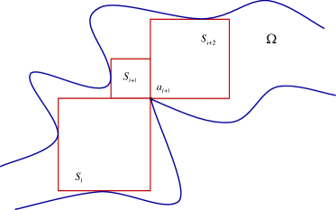
Figure 14:  

Proof. Let us prove part (i) of the lemma. Note that $S_{i}^{\operatorname{\,cl}}\cap S_{i+1}^{\operatorname{\,cl}}$ is a line segment because $S_{i}$ and $S_{i+1}$ are touching squares such that $\#(S_{i}^{\operatorname{\,cl}}\cap S_{i+1}^{\operatorname{\,cl}})>1$.

Prove that $(u_{i},v_{i})\subset\Omega$. In fact, $(u_{i},v_{i})\cap\Omega$ is an open set in the relative topology of the straight line passing through $u_{i}$ and $v_{i}$. By part (ii) of Theorem 1.9, this set is non-empty, so that $(u_{i},v_{i})\cap\Omega$ can be represented as a union of a finite or countable family ${\mathcal{I}}$ of pairwise disjoint open subintervals of $(u_{i},v_{i})$ with ends in $\partial\Omega$.

Let us show that this family contains precisely one subinterval of $(u_{i},v_{i})$, i.e., $\#{\mathcal{I}}=1$. Suppose that it is not true, i.e., that there exist two distinct line intervals from this family, say $I^{\prime}=(x^{\prime},y^{\prime})$ and $I^{\prime\prime}=(x^{\prime\prime},y^{\prime\prime})$, $I^{\prime}\neq I^{\prime\prime}$. Then $x^{\prime},y^{\prime},x^{\prime\prime},y^{\prime\prime}\in\partial\Omega$ and $I^{\prime}\cup I^{\prime\prime}\subset(u_{i},v_{i})\cap\Omega$. See Figure 15.

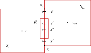
Figure 15:  

We may assume that $y^{\prime},x^{\prime\prime}\in(x^{\prime},y^{\prime\prime})$. Then there exists a rectangle $R$ with sides parallel to the coordinate axes and width small enough such that $y^{\prime},x^{\prime\prime}\subset R\hskip 0.56905pt^{\circ}$ and $\partial R\subset\Omega$. See Figure 15. Since $\Omega$ is simply connected, $R\subset\Omega$ so that $y^{\prime}\in\Omega$. But $y^{\prime}\in\partial\Omega$, a contradiction.

Thus $\#{\mathcal{I}}=1$ so that

$$(u_{i},v_{i})\cap\Omega=(z^{\prime},z^{\prime\prime})~{}~{}\text{for some}~{}~{}z^{\prime},z^{\prime\prime}\in[u_{i},v_{i}].$$

We may assume that

$$\|z^{\prime}-u_{i}\|<\|z^{\prime\prime}-u_{i}\|~{}~{}~{}\text{and}~{}~{}~{}~{}~{}~{}\|z^{\prime\prime}-v_{i}\|<\|z^{\prime}-v_{i}\|.$$

Prove that $z^{\prime}=u_{i}$ and $z^{\prime\prime}=v_{i}$. Suppose that it is not true, and, for instance, $z^{\prime}\neq u_{i}$. Then the line segment $[u_{i},z^{\prime}]\subset\partial\Omega$.

Let $\widetilde{z}:=(u_{i}+z^{\prime})/2$. Then there exist sequences $\{a_{j}\}_{j=1}^{\infty}\subset S_{i}$ and $\{b_{j}\}_{j=1}^{\infty}\subset S_{i+1}$ such that

$$a_{j}\to\widetilde{z}~{}~{}\text{and}~{}~{}b_{j}\to\widetilde{z}~{}~{}\text{as}~{}~{}j\to\infty.$$

Since $[u_{i},z^{\prime}]\subset\partial\Omega$, any path $\gamma$ joining $a_{j}$ to $b_{j}$ in $\Omega$ has the diameter at least $\|u_{i}-z^{\prime}\|/8$ provided $a_{j}$ and $b_{j}$ are close enough to $\widetilde{z}$. On the other hand, $\Omega$ satisfies condition (4.1) so that, by Theorem 4.1, the points $a_{j}$ and $b_{j}$ can be joined by a certain path $\gamma_{j}$ such that

$$\operatorname{diam}\gamma_{j}\leq\eta\|a_{j}-b_{j}\|.$$

Hence,

$$\|a_{i}-z^{\prime}\|/8\leq\operatorname{diam}\gamma_{j}\leq\eta\|a_{j}-b_{j}\|\to 0~{}~{}\text{as}~{}~{}j\to\infty.$$

Since $a_{j}\to\widetilde{z}$, we have $\widetilde{z}=z^{\prime}$ so that $z^{\prime}=u_{i}$, a contradiction. In the same fashion we prove that $z^{\prime\prime}=v_{i}$ so that $(u_{i},v_{i})=(z^{\prime},z^{\prime\prime})\subset\Omega$.

Finally, we obtain that

$$(S_{i}^{\operatorname{\,cl}}\cup S_{i+1}^{\operatorname{\,cl}})^{\circ}=S_{i}\cup S_{i+1}\cup(u_{i},v_{i})\subset\Omega$$

proving part (i) of the lemma.

Prove part (ii) and (iii). First prove that

$$\#(S_{i}^{\operatorname{\,cl}}\cap S_{j}^{\operatorname{\,cl}})\leq 1~{}~{}~{}\text{provided}~{}~{}~{}|i-j|>1,~{}1\leq i,j\leq k.$$ (4.5)

Suppose that $1\leq i<j\leq k$ and $S_{i}^{\operatorname{\,cl}}\cap S_{j}^{\operatorname{\,cl}}\neq\emptyset$.

Since $S_{i}\cap S_{j}=\emptyset$, we have $S_{i}^{\operatorname{\,cl}}\cap S_{j}^{\operatorname{\,cl}}=\partial S_{i}\cap\partial S_{j}$ so that

$$S_{i}^{\operatorname{\,cl}}\cap S_{j}^{\operatorname{\,cl}}=[a,b]~{}~{}~{}\text{for some}~{}~{}~{}a,b\in{\bf R}^{2}.$$ (4.6)

We know that $S_{i}^{\operatorname{\,cl}}\cap S_{j}^{\operatorname{\,cl}}\cap\Omega=\emptyset$ whenever $|i-j|>1$, see part (ii) of Lemma 3.4. Hence $[a,b]\subset{\bf R}^{2}\setminus\Omega$. On the other hand, by (4.6), $[a,b]\subset\Omega^{\operatorname{\,cl}}$ so that $[a,b]\subset\partial\Omega$.

Let us assume that $\#(S_{i}^{\operatorname{\,cl}}\cap S_{j}^{\operatorname{\,cl}})>1$, i.e., that $a\neq b$. Let $z:=(a+b)/2$. Since $z\in S_{i}^{\operatorname{\,cl}}\cap S_{j}^{\operatorname{\,cl}}$, there exist sequences of points

$$\{s_{n}\}_{n=1}^{\infty}\subset S_{i}~{}~{}~{}\text{and}~{}~{}~{}\{t_{n}\}_{n=1}^{\infty}\subset S_{j}~{}~{}~{}\text{such that}~{}~{}~{}s_{n},t_{n}\to z~{}~{}~{}\text{as}~{}~{}~{}n\to\infty.$$ (4.7)

Since $\Omega$ satisfies condition (4.1) and $s_{n},t_{n}\to z$, by Theorem 4.1, there exists a path $\gamma_{n}$ connecting $s_{n}$ to $t_{n}$ in $\Omega$ such that

$$\operatorname{diam}\gamma_{n}\leq\eta\|s_{n}-t_{n}\|$$ (4.8)

provided $n>N$ where $N$ is big enough. We may also assume that $N$ is so big that

$$\|z-s_{n}\|<\|a-b\|/(8\eta)~{}~{}~{}\text{and}~{}~{}~{}\|z-t_{n}\|<\|a-b\|/(8\eta)~{}~{}~{}\text{for}~{}~{}~{}n>N.$$ (4.9)

Note that the straight line passing through $a$ and $b$ separates $s_{n}$ and $t_{n}$ and the path $\gamma_{n}$ does not cross the line segment $[a,b]$. Therefore

$$\operatorname{diam}\gamma_{n}\geq\tfrac{1}{2}\|a-b\|-\tfrac{1}{8}\|a-b\|=\tfrac{3}{8}\|a-b\|.$$ (4.10)

On the other hand, by (4.8) and (4.9),

$$\operatorname{diam}\gamma_{n}\leq\eta\|s_{n}-t_{n}\|\leq\eta(\|z-s_{n}\|+\|z-t_{n}\|)\leq 2\eta\,\frac{\|a-b\|}{8\eta}=\tfrac{1}{4}\|a-b\|.$$

This inequality contradicts to inequality (4.10) proving (4.5).

Now suppose that

$$S_{i}^{\operatorname{\,cl}}\cap S_{j}^{\operatorname{\,cl}}\neq\emptyset~{}~{}~{}\text{for some}~{}~{}~{}1\leq i<j\leq k,$$

and prove that this condition is satisfied only for $j=i+2$.

In fact, by (4.5), $S_{i}^{\operatorname{\,cl}}\cap S_{j}^{\operatorname{\,cl}}=\{a\}$ for some $a\in\partial\Omega\cap\partial S_{i}\cap\partial S_{j}$. Prove that

$$a\in S_{\ell}^{\operatorname{\,cl}}~{}~{}~{}\text{for every}~{}~{}~{}i\leq\ell\leq j.$$ (4.11)

As above, by $\{s_{n}\}_{n=1}^{\infty}$ and $\{t_{n}\}_{n=1}^{\infty}$ we denote the sequences of points satisfying (4.7), and by $\gamma_{n}$ we denote a path joining $s_{n}$ to $t_{n}$ in $\Omega$ such that (4.8) holds. Then, by part (i) of Lemma 3.4,

$$\gamma_{n}\cap S_{\ell}\neq\emptyset~{}~{}~{}\text{for every}~{}~{}~{}\ell,~{}i\leq\ell\leq j.$$

Let $b^{(n)}_{\ell}\in\gamma_{n}\cap S_{\ell}$, $i<\ell<j$. We also put $b^{(n)}_{i}:=s_{n}$ and $b^{(n)}_{j}:=t_{n}$. Then, by (4.8),

$$\|b^{(n)}_{\ell}-s_{n}\|\leq\operatorname{diam}\gamma_{n}\leq\eta\|s_{n}-t_{n}\|.$$

Since $\|s_{n}-t_{n}\|\to 0$ and $s_{n}\to a$ as $n\to\infty$, we conclude that $b^{(n)}_{\ell}\to a$ for every $\ell,i\leq\ell\leq j$. Hence, $a\in S^{\operatorname{\,cl}}_{\ell}$ proving (4.11).

Thus, by (4.5) and (4.11), if $i+2\leq j\leq k$ and $S_{i}^{\operatorname{\,cl}}\cap S_{j}^{\operatorname{\,cl}}\neq\emptyset$, then there exists a point $a\in\partial S_{i}$ such that

$$S_{i}^{\operatorname{\,cl}}\cap S_{\ell}^{\operatorname{\,cl}}=\{a\}~{}~{}~{}\text{for all}~{}~{}~{}\ell,~{}i\leq\ell\leq j.$$ (4.12)

Since $\{S_{\ell}:i\leq\ell\leq j\}$ are pairwise disjoint squares, this property easily implies the required restriction $j=i+2$. In fact, since $S_{i}\cap S_{\ell}=\emptyset$ and

$$S_{i}^{\operatorname{\,cl}}\cap S_{\ell}^{\operatorname{\,cl}}=\{a\},$$

the point $a$ is a vertex of the square $S_{\ell}$ for every $\ell,~{}i\leq\ell\leq j$. In particular, $a$ is a common vertex of $S_{i}$ and $S_{i+2}$. Note that, by (4.12), $a\in S_{i+1}^{\operatorname{\,cl}}$. Since $S_{i},S_{i+1},S_{i+2}$ are pairwise disjoint squares, this implies that the point $a_{i+1}=a$ is a vertex of the square $S_{i+1}$ as well.

By part (ii) of Lemma 3.4, $S^{\operatorname{\,cl}}_{i}\cap S^{\operatorname{\,cl}}_{i+2}\cap\Omega=\emptyset$ so that $a\in\partial\Omega$. It is also clear that $a$ is a boundary point of the set $S^{\operatorname{\,cl}}_{i}\cup S^{\operatorname{\,cl}}_{i+1}\cup S^{\operatorname{\,cl}}_{i+2}$. See Figure 16.

Figure 16:  

But, $a$ is also a vertex of the square $S_{j}$. Since $S_{i},S_{i+1},S_{i+2}$ and $S_{j}$ are pairwise disjoint squares, and $a$ is a common vertex of these squares, the intersection of $S_{i}^{\operatorname{\,cl}}$ and $S_{j}^{\operatorname{\,cl}}$ is a line segment (of positive length). See Figure 16.

Thus $\#(S_{i}^{\operatorname{\,cl}}\cap S_{j}^{\operatorname{\,cl}})>1$ whenever $j>i+2$ which contradicts (4.5). Hence, $S_{i}^{\operatorname{\,cl}}\cap S_{j}^{\operatorname{\,cl}}=\emptyset$ provided $|i-j|>2$.

The proof of the lemma is complete.         $\Box$

Part (iii) of Lemma 4.2 motivates us to introduce the following

Definition 4.3

Let $1\leq i\leq k-1$ and let $a_{i+1}\in\partial\Omega$ be a common vertex of the squares $S^{\operatorname{\,cl}}_{i},S^{\operatorname{\,cl}}_{i+1}$ and $S^{\operatorname{\,cl}}_{i+2}$, i.e.,

$$\{a_{i+1}\}=S^{\operatorname{\,cl}}_{i}\cap S^{\operatorname{\,cl}}_{i+1}\cap S^{\operatorname{\,cl}}_{i+2}.$$

We refer to the point $a_{i+1}$ as a rotation point of “The Wide Path” ${\mathcal{W}}={\cal WP}_{\Omega}^{(\bar{x},\bar{y})}$, and to the square $S_{i+1}$ as a rotation square of ${\mathcal{W}}$.

See Figure 14. Another example is given on Figure 17.

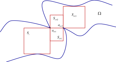
Figure 17:  

Here $\{a_{i+1}\}$ and $\{a_{i+2}\}$ are the rotation points corresponding to the rotation squares $S_{i+1}$ and $S_{i+2}$. Note that rotation points and rotation squares play an important in construction of “The Narrow path”. See Section 5.

4.2. Subhyperbolic properties of elementary squarish domains. We will be needed several auxiliary results related to subhyperbolic properties of domains in ${\bf R}^{2}$ consisting of a “small number” of open squares. We refer to such sets as “elementary squarish domains”.

Lemma 4.4

Let $Q$ be a square in ${\bf R}^{2}$ and let $a,b\in Q^{\operatorname{\,cl}}$. Then there exists a path $\gamma_{ab}$ joining $a$ to $b$ and consisting of at most two edges such that $\gamma_{ab}\setminus\{a,b\}\subset Q$ and for every $\alpha\in(0,1]$ the following inequality

$$\operatorname{len}_{\alpha,Q}(\gamma_{ab})\leq\tfrac{3}{\alpha}\,\|a-b\|^{\alpha}$$ (4.13)

holds. See (1.4).

Proof. Let $a=(a_{1},a_{2})$, $b=(b_{1},b_{2})$ and let $Q=(u_{1},u_{2})\times(v_{1},v_{2})$. Suppose that $|a_{2}-b_{2}|\leq|a_{1}-b_{1}|=\|a-b\|$. Since $a_{2},b_{2}\in[v_{1},v_{2}]$ and

$$|v_{1}-v_{2}|=\operatorname{diam}Q\geq\|a-b\|\geq|a_{2}-b_{2}|$$

there exists a line segment $[s_{1},s_{2}]$ such that

$$a_{2},b_{2}\in[s_{1},s_{2}]\subset[v_{1},v_{2}]~{}~{}~{}\text{and}~{}~{}~{}|s_{1}-s_{2}|=|a_{1}-b_{1}|=\|a-b\|.$$

Let $Q_{ab}:=(a_{1},b_{1})\times(s_{1},s_{2})$. Then $Q_{ab}\subset Q$, $a,b\in\partial Q_{ab}$ and $\operatorname{diam}Q_{ab}=\|a-b\|$. Let $Q_{ab}=S(c,r)$, i.e., $c$ is the center of $Q_{ab}$ and $r=\tfrac{1}{2}\|a-b\|$ is its “radius”, and let

$$\gamma_{ab}:=[a,c]\cup[c,b].$$

Clearly, $\gamma_{ab}$ is a two edges path connecting $a$ to $b$ such that $\gamma_{ab}\setminus\{a,b\}\subset Q$.

Prove inequality (4.13). By definition (1.4),

$$\operatorname{len}_{\alpha,Q}(\gamma_{ab}) := \int\limits_{\gamma_{ab}}\operatorname{dist}(z,\partial Q)^{\alpha-1}\,ds(z)$$

$$\leq \int\limits_{[a,c]}\operatorname{dist}(z,\partial Q_{ab})^{\alpha-1}\,ds(z)+\int\limits_{[c,b]}\operatorname{dist}(z,\partial Q_{ab})^{\alpha-1}\,ds(z)$$

$$= I_{1}+I_{2}.$$

Note that $\operatorname{dist}(z,\partial Q_{ab})=\|z-a\|$ for every $z\in[a,c]$. Hence,

$$I_{1}:=\int\limits_{[a,c]}\operatorname{dist}(z,\partial Q_{ab})^{\alpha-1}\,ds(z)=\int\limits_{[a,c]}\|z-a\|^{\alpha-1}\,ds(z)=\int\limits_{0}^{1}(\|a-c\|\,t)^{\alpha-1}\|a-c\|_{2}\,dt$$

where $\|\cdot\|_{2}$ denotes the Euclidean norm in ${\bf R}^{2}$.

Recall that $a\in\partial Q_{ab}$ so that

$$\|a-c\|=r=\tfrac{1}{2}\operatorname{diam}Q_{ab}=\tfrac{1}{2}\,\|a-b\|.$$

We obtain:

$$I_{1}\leq r^{\alpha-1}(\sqrt{2}r)\,\int\limits_{0}^{1}\,t^{\alpha-1}\,dt=\tfrac{\sqrt{2}}{\alpha}\,r^{\alpha}.$$

In the same way we prove that

$$I_{2}:=\int\limits_{[c,b]}\operatorname{dist}(z,\partial Q_{ab})^{\alpha-1}\,ds(z)\leq\tfrac{\sqrt{2}}{\alpha}\,r^{\alpha}.$$

Hence,

$$\operatorname{len}_{\alpha,Q}(\gamma_{ab})\leq I_{1}+I_{2}\leq\tfrac{2\sqrt{2}}{\alpha}\,r^{\alpha}=\tfrac{2\sqrt{2}}{\alpha\,2^{\alpha}}\,\|a-b\|^{\alpha}\leq\tfrac{3}{\alpha}\,\|a-b\|^{\alpha}.$$

The proof of the lemma is complete.         $\Box$

Lemma 4.5

Let $Q_{1}$ and $Q_{2}$ be squares in ${\bf R}^{2}$ such that $\#(Q_{1}^{\operatorname{\,cl}}\cap Q_{2}^{\operatorname{\,cl}})>1$, and let

$$G:=(Q_{1}^{\operatorname{\,cl}}\cup Q_{2}^{\operatorname{\,cl}})^{\circ}.$$

Then for every $a,b\in G^{\operatorname{\,cl}}$, $a\neq b$, there exists a path $\gamma_{ab}(G)$ consisting of at most four edges which joins $a$ to $b$ in $G$ such that $\gamma_{ab}(G)\setminus\{a,b\}\subset G$ and for every $\alpha\in(0,1]$

$$\operatorname{len}_{\alpha,G}(\gamma_{ab}(G))\leq\tfrac{12}{\alpha}\,\|a-b\|^{\alpha}.$$ (4.14)

Proof. Suppose that $a\in Q_{1}^{\operatorname{\,cl}}$ and $b\in Q_{2}^{\operatorname{\,cl}}$. If $a,b\in Q_{1}^{\operatorname{\,cl}}$ or $a,b\in Q_{2}^{\operatorname{\,cl}}$, then the lemma directly follows from Lemma 4.4. Thus we can assume that $a\in Q_{1}^{\operatorname{\,cl}}\setminus Q_{2}^{\operatorname{\,cl}}$ and $b\in Q_{2}^{\operatorname{\,cl}}\setminus Q_{1}^{\operatorname{\,cl}}$.

Let $a=(a_{1},a_{2}),b=(b_{1},b_{2})$ and let

$$\Pi(a,b):=[a_{1},b_{1}]\times[a_{2},b_{2}].$$

Thus $\Pi(a,b)$ is the smallest closed rectangle with sides parallel to the coordinate axes containing $a$ and $b$. Then by Helly’s intersection theorem for rectangles

$$Q_{1}^{\operatorname{\,cl}}\cap Q_{2}^{\operatorname{\,cl}}\cap\Pi(a,b)\neq\emptyset.$$

Let $\widetilde{w}\in Q_{1}^{\operatorname{\,cl}}\cap Q_{2}^{\operatorname{\,cl}}\cap\Pi(a,b)$. Since $\widetilde{w}\in\Pi(a,b)$, we have

$$\|a-\widetilde{w}\|,\|b-\widetilde{w}\|\leq\|a-b\|.$$ (4.15)

Let $R:=G\cap Q_{1}^{\operatorname{\,cl}}\cap Q_{2}^{\operatorname{\,cl}}$. Then $R$ is either an open line interval or an open rectangle. In both cases $\widetilde{w}\in R^{\operatorname{\,cl}}$ so that there exists $w\in R$ such that $\|\widetilde{w}-w\|<\|a-b\|$. By this inequality and (4.15),

$$\|a-w\|,\|b-w\|\leq 2\|a-b\|.$$ (4.16)

Since $w\in Q_{1}^{\operatorname{\,cl}}$, by Lemma 4.4, there exists a path $\gamma_{1}$ (consisting of at most two edges) which joins $a$ to $w$ such that $\gamma_{1}\setminus\{a,w\}\subset Q_{1}$ and

$$\operatorname{len}_{\alpha,Q_{1}}(\gamma_{1})\leq\tfrac{3}{\alpha}\,\|a-w\|^{\alpha}.$$

In a similar way we construct a path $\gamma_{2}$ (consisting of at most two edges) which connects $b$ to $w$ such that $\gamma_{2}\setminus\{b,w\}\subset Q_{2}$ and

$$\operatorname{len}_{\alpha,Q_{2}}(\gamma_{2})\leq\tfrac{3}{\alpha}\,\|b-w\|^{\alpha}.$$

Since $Q_{i}\subset G$, we have $\operatorname{dist}(z,\partial Q_{i})\leq\operatorname{dist}(z,\partial G)$ for every $z\in Q_{i}$, so that, by definition 1.4, $\operatorname{len}_{\alpha,G}(\gamma_{i})\leq\operatorname{len}_{\alpha,Q_{i}}(\gamma_{i})$, $i=1,2$. Hence,

$$\operatorname{len}_{\alpha,G}(\gamma_{1})\leq\tfrac{3}{\alpha}\,\|a-w\|^{\alpha}~{}~{}~{}\text{and}~{}~{}~{}\operatorname{len}_{\alpha,G}(\gamma_{2})\leq\tfrac{3}{\alpha}\,\|b-w\|^{\alpha}.$$

Let $\gamma_{ab}(G):=\gamma_{1}\cup\gamma_{2}$. Then $\gamma_{ab}(G)$ is a path consisting of at most four edges which connects $a$ to $b$ in $G$ such that

$$\operatorname{len}_{\alpha,G}(\gamma_{ab}(G))=\operatorname{len}_{\alpha,G}(\gamma_{1})+\operatorname{len}_{\alpha,G}(\gamma_{2})\leq\tfrac{3}{\alpha}\,\|a-w\|^{\alpha}+\tfrac{3}{\alpha}\,\|b-w\|^{\alpha}.$$

This inequality and (4.16) imply (4.14) proving the lemma.         $\Box$

Lemma 4.6

(i). Let $G\subset{\bf R}^{2}$ be one of the following sets:

(a). $G=(Q_{1}^{\operatorname{\,cl}}\cup Q_{2}^{\operatorname{\,cl}})^{\circ}$ where $Q_{1}$ and $Q_{2}$ are disjoint squares such that $\#(Q_{1}^{\operatorname{\,cl}}\cap Q_{2}^{\operatorname{\,cl}})>1;$

(b). $G=Q_{1}\cup Q_{2}\cup Q_{3}$ where $Q_{1}$ and $Q_{2}$ are disjoint squares such that $Q_{1}^{\operatorname{\,cl}}\cap Q_{2}^{\operatorname{\,cl}}$ is a singleton, and $Q_{3}$ is a square centered at $Q_{1}^{\operatorname{\,cl}}\cap Q_{2}^{\operatorname{\,cl}}$.

Then $G$ is an $\alpha$-subhyperbolic domain for every $\alpha\in(0,1]$. See Definition 1.4. Furthermore, for every $a,b\in G^{\operatorname{\,cl}}$, $a\neq b$, there exists a path $\gamma_{ab}(G)$ which joins $a$ to $b$ in $G$ such that $\gamma_{ab}(G)\setminus\{a,b\}\subset G$ and for every $\alpha\in(0,1]$

$$\operatorname{len}_{\alpha,G}(\gamma_{ab}(G))\leq\tfrac{12}{\alpha}\,\|a-b\|^{\alpha}\,;$$ (4.17)

(ii). Every domain $G$ satisfying either condition (a) or condition (b) is a Sobolev $L^{m}_{p}$-extension domain with $e(L^{m}_{p}(G))\leq C(m,p)$. See (1.2).

Proof. If $G$ satisfies condition of part (a), then the statement (i) of the lemma directly follows from Definition 1.4 and Lemma 4.5.

Let $G$ be a domain from part (b) of the lemma, and let $a,b\in G^{\operatorname{\,cl}}$. If $a,b\in Q_{1}^{\operatorname{\,cl}}\cup Q_{3}^{\operatorname{\,cl}}$ or $a,b\in Q_{2}^{\operatorname{\,cl}}\cup Q_{3}^{\operatorname{\,cl}}$, then, by Lemma 4.5, there exists a path $\gamma_{ab}(G)$ satisfying inequality (4.17).

Now suppose that $a\in Q_{1}^{\operatorname{\,cl}}\setminus Q_{3}$ and $b\in Q_{2}^{\operatorname{\,cl}}\setminus Q_{3}^{\operatorname{\,cl}}$. Let $c$ be the center of the square $Q_{3}$, i.e., $\{c\}=Q_{1}^{\operatorname{\,cl}}\cap Q_{2}^{\operatorname{\,cl}}$. Then, by Lemma 4.4, there exists a path $\gamma_{ac}$ joining $a$ to $c$ such that $\gamma_{ac}\setminus\{a,c\}\subset Q_{1}$ and $\operatorname{len}_{\alpha,Q_{1}}(\gamma_{ac})\leq\tfrac{3}{\alpha}\,\|a-c\|^{\alpha}$. In the same way we prove the existence of a path $\gamma_{cb}$ joining $c$ to $b$ such that $\gamma_{cb}\setminus\{b,c\}\subset Q_{2}$ and $\operatorname{len}_{\alpha,Q_{2}}(\gamma_{cb})\leq\tfrac{3}{\alpha}\,\|b-c\|^{\alpha}$.

Let $\gamma_{ab}(G):=\gamma_{ac}\cup\gamma_{cb}$. Since $Q_{1},Q_{2}\subset G$,

$$\operatorname{len}_{\alpha,G}(\gamma_{ab}(G))=\operatorname{len}_{\alpha,G}(\gamma_{ac})+\operatorname{len}_{\alpha,G}(\gamma_{cb})\leq\operatorname{len}_{\alpha,Q_{1}}(\gamma_{ac})+\operatorname{len}_{\alpha,Q_{2}}(\gamma_{cb})$$

so that

$$\operatorname{len}_{\alpha,G}(\gamma_{ab}(G))\leq\tfrac{3}{\alpha}\,(\|a-c\|^{\alpha}+\|b-c\|^{\alpha}).$$

Clearly, $c\in\Pi(a,b)$ where $\Pi(a,b):=[a_{1},b_{1}]\times[a_{2},b_{2}]$ provided $a=(a_{1},a_{2})$ and $b=(b_{1},b_{2})$. Hence

$$\|a-c\|,\|b-c\|\leq\|a-b\|~{}~{}~{}\text{so that}~{}~{}~{}\operatorname{len}_{\alpha,G}(\gamma_{ab}(G))\leq\tfrac{6}{\alpha}\,\|a-b\|^{\alpha}$$

proving inequality (4.17) and part (i) of the lemma.

It remains to note that part (ii) of the lemma directly follows from part (i) of the present lemma and Theorem 1.7.

The proof of the lemma is complete.         $\Box$

4.3. Main geometrical properties of “The Wide Path”. Let us give a precise definition of the family of sets $\{\widehat{S}_{i}:1\leq i\leq k\}$ which we have used in definition (1.18) of “The Wide Path”. See Section 1.

Definition 4.7

We put

$$\widehat{S}_{i}:=\emptyset~{}~{}\text{if}~{}~{}i=k~{}~{}\text{or}~{}~{}\#(S_{i}^{\operatorname{\,cl}}\cap S_{i+1}^{\operatorname{\,cl}})>1\,.$$ (4.18)

We also put

$$\widehat{S}_{i}:=S(w_{i},\hat{\delta})~{}~{}~{}\text{if}~{}~{}~{}\#(S_{i}^{\operatorname{\,cl}}\cap S_{i+1}^{\operatorname{\,cl}})=1$$ (4.19)

where

$$\{w_{i}\}:=S_{i}^{\operatorname{\,cl}}\cap S_{i+1}^{\operatorname{\,cl}}$$ (4.20)

and

$$\hat{\delta}:=\tfrac{1}{8}\min\{\hat{\delta}_{1},\hat{\delta}_{2},\hat{\delta}_{3}\}.$$ (4.21)

Here  $\hat{\delta}_{1}:=\min\{\operatorname{dist}(w_{m},\partial\Omega):m\in I\}$,  $\hat{\delta}_{2}:=\min\{\operatorname{diam}S_{m}:1\leq m\leq k\}$, and

$$\hat{\delta}_{3}:=\min\{\operatorname{dist}(w_{m},S_{j}):m\in I,1\leq j\leq k,j\neq m,m+1\}$$ (4.22)

where

$$I:=\{m\in\{1,...,k-1\}:\#(S_{m}^{\operatorname{\,cl}}\cap S_{m+1}^{\operatorname{\,cl}})=1\}.$$

Prove that $\hat{\delta}>0$, i.e., that the squares $\widehat{S}_{i}$ in (4.19) are well defined. In fact, since $w_{i}\in[c_{i},c_{i+1}]$, $i\in I$, by inclusion (3.1), $w_{i}\in\Omega$. (Recall that $c_{i}$ denotes the center of the square $S_{i}$.) Hence, $\hat{\delta}_{1}>0$. It is also clear that $\hat{\delta}_{2}>0$. By part(ii) of Lemma 3.4, $w_{i}\notin S_{j}^{\operatorname{\,cl}}$ whenever $j\neq i,i+1$, so that $\hat{\delta}_{3}>0$ as well. Hence, $\hat{\delta}>0$.

Our proof of the Sobolev extension property of “The Wide Path”

$${\mathcal{W}}:={\cal WP}_{\Omega}^{(\bar{x},\bar{y})}$$

relies on a series of results which describe a geometrical structure of ${\mathcal{W}}$ and its complement ${\mathcal{H}}:=\Omega\setminus{\mathcal{W}}.$ Let us recall that

$${\mathcal{W}}=\left(\,\bigcup_{i=1}^{k}\left(\,S_{i}^{\operatorname{\,cl}}\,{\bigcup}\,\widehat{S}_{i}\,\right)\right)^{\circ}\,.$$ (4.23)

In the next lemma we present several useful properties of the sets $\widehat{S}_{i}$ which directly follow from Definition 4.7.

Lemma 4.8

Let $\bar{x},\bar{y}\in\Omega$ and let $S_{i},S_{i+1}\in{\mathcal{S}}_{\Omega}(\bar{x},\bar{y})$ be two squares such that $S_{i}^{\operatorname{\,cl}}\cap S_{i+1}^{\operatorname{\,cl}}$ is a singleton. Then

$$\operatorname{diam}\widehat{S}_{i}\leq\tfrac{1}{4}\min\{\operatorname{diam}S_{i},\operatorname{diam}S_{i+1}\}.$$

Furthermore, the sets of the family $\{2\widehat{S}_{i}:1=1,...,k\}$ are pairwise disjoint subsets of $\Omega$ satisfying the following condition:

$$(2\widehat{S}_{i}^{\operatorname{\,cl}})\cap S_{j}^{\operatorname{\,cl}}=\emptyset~{}~{}\text{for every}~{}~{}1\leq i,j\leq k,~{}j\neq i,i+1.$$ (4.24)

In particular,

$$\operatorname{diam}\widehat{S}_{i}\leq 2\operatorname{dist}(\widehat{S}_{i},S_{j})~{}~{}~{}\text{for all}~{}~{}~{}1\leq i,j\leq k,~{}j\neq i,i+1,$$

and

$$\operatorname{diam}\widehat{S}_{i}+\operatorname{diam}\widehat{S}_{j}\leq 4\operatorname{dist}(\widehat{S}_{i},\widehat{S}_{j})~{}~{}~{}\text{for all}~{}~{}~{}1\leq i,j\leq k,~{}j\neq i.$$

Proposition 4.9

“The Wide Path” ${\mathcal{W}}:={\cal WP}_{\Omega}^{(\bar{x},\bar{y})}$ is an open connected subset of $\Omega$ which has the following representation:

$${\mathcal{W}}=\bigcup_{i=1}^{k-1}\left(\,S_{i}^{\operatorname{\,cl}}\,{\bigcup}\,S_{i+1}^{\operatorname{\,cl}}\,{\bigcup}\,\widehat{S}_{i}\,\right)^{\circ}\,.$$ (4.25)

Proof. Let

$$\widetilde{W}:=\bigcup_{i=1}^{k-1}\left(\,S_{i}^{\operatorname{\,cl}}\,{\bigcup}\,S_{i+1}^{\operatorname{\,cl}}\,{\bigcup}\,\widehat{S}_{i}\,\right)^{\circ}\,.$$

Clearly, ${\mathcal{W}}\supset(S_{i}^{\operatorname{\,cl}}\cup S_{i+1}^{\operatorname{\,cl}}\cup\widehat{S}_{i})^{\circ}$ for every $i=1,...,k-1,$ so that ${\mathcal{W}}\supset\widetilde{W}$.

Prove that ${\mathcal{W}}\subset\widetilde{W}$. Let $a\in{\mathcal{W}}$. Then, by (4.23), there exists $\delta>0$ such that

$$S(a,\delta)\subset\,\bigcup_{j=1}^{k}\,\left(\,S_{j}^{\operatorname{\,cl}}\,{\bigcup}\,\widehat{S}_{j}\,\right)\,.$$ (4.26)

Let us consider the following two cases.

The first case. There exists $i\in\{1,...,k-1\}$ such that $a\in 2\widehat{S}_{i}^{\operatorname{\,cl}}$.

By Lemma 4.8, $(2\widehat{S}_{i})\cap(2\widehat{S}_{j})=\emptyset$ for every $j\neq i,1\leq j\leq k$. Furthermore, by (4.24),

$$(2\widehat{S}_{i}^{\operatorname{\,cl}})\cap S_{j}^{\operatorname{\,cl}}\neq\emptyset~{}~{}~{}\text{if and only if}~{}~{}~{}j=i~{}~{}~{}\text{or}~{}~{}~{}j=i+1.$$ (4.27)

Hence, $a\notin 2\widehat{S}_{j}^{\operatorname{\,cl}}$ provided $j\neq i$ so that

$$\eta_{1}:=\tfrac{1}{2}\,\min\{\operatorname{dist}(a,\widehat{S}_{j}^{\operatorname{\,cl}}):1\leq j\leq k,j\neq i\,\}\,>0.$$

Thus the square $S(a,\eta_{1})$ does not cross any square $\widehat{S}_{j}$ whenever $j\neq i$.

Also note that, by (4.27),

$$\eta_{2}:=\tfrac{1}{2}\,\min\{\operatorname{dist}(a,S_{j}^{\operatorname{\,cl}}):1\leq j\leq k,j\neq i,i+1\,\}\,>0.$$ (4.28)

Let $\widetilde{\delta}:=\min\{\delta,\eta_{1},\eta_{2}\}$. Then the $\widetilde{\delta}$-neighborhood of $a$, the square $S(a,\widetilde{\delta})$, may contain only points from the squares $S_{i}^{\operatorname{\,cl}},S_{i+1}^{\operatorname{\,cl}}$ and $\widehat{S}_{i}$. Hence, by (4.26),

$$a\in\left(S_{i}^{\operatorname{\,cl}}\,{\bigcup}\,S_{i+1}^{\operatorname{\,cl}}\,{\bigcup}\,\widehat{S}_{i}\,\right)^{\circ}\subset\widetilde{W}.$$

The second case. Let $a\in{\mathcal{W}}$ but $a\notin 2\widehat{S}_{j}$ for every $j,1\leq j\leq k$. In particular,

$$a\notin\widehat{S}_{j}^{\operatorname{\,cl}}~{}~{}\text{for every}~{}~{}1\leq j\leq k.$$

Since

$$a\in{\mathcal{W}}\subset\bigcup_{i=1}^{k}\,(S_{i}^{\operatorname{\,cl}}\,{\bigcup}\,\widehat{S}_{i})$$

we conclude that there exists $i\in\{1,...,k\}$ such that $a\in S_{i}^{\operatorname{\,cl}}\cap\Omega$.

By part (ii) and (iii) of Lemma 4.2, we may choose the index $i$ in such a way that either

$$a\in S_{i}^{\operatorname{\,cl}}\cup S_{i+1}^{\operatorname{\,cl}}~{}~{}\text{and}~{}~{}a\notin S_{j}^{\operatorname{\,cl}}~{}~{}\text{for every}~{}~{}j\neq i,i+1,$$ (4.29)

or

$$\{a\}=\{a_{i+1}\}=S_{i}^{\operatorname{\,cl}}\cap S_{i+1}^{\operatorname{\,cl}}\cap S_{i+2}^{\operatorname{\,cl}}~{}\text{and}~{}a~{}\text{is a common vertex of}~{}S_{i},S_{i+1},S_{i+2}\,.$$ (4.30)

Furthermore, in this case

$$a\notin S_{j}^{\operatorname{\,cl}}~{}~{}\text{for every}~{}~{}j\neq i,i+1,i+2,$$ (4.31)

and $a$ is a boundary point of the set $S^{\operatorname{\,cl}}_{i}\cup S^{\operatorname{\,cl}}_{i+1}\cup S^{\operatorname{\,cl}}_{i+2}$. In other words, $a=a_{i+1}$ is a rotation point of “The Wide Path” ${\mathcal{W}}$, and the square $S_{i+1}$ is its rotation square associated with $a_{i+1}$. See Definition 4.3.

We begin with the first case described by (4.29). In this case the quantity $\eta_{2}$ defined by (4.28) is positive. Note that the following quantity

$$\rho_{1}:=\tfrac{1}{2}\,\min\{\operatorname{dist}(a,\widehat{S}_{j}^{\operatorname{\,cl}}):1\leq j\leq k\,\}$$

is positive as well.

Let $\rho:=\min\{\delta,\eta_{2},\rho_{1}\}$. Clearly, $\rho>0$. Then the $\rho$-neighborhood of $a$, the square $S(a,\rho)$, does not intersect $S_{j}^{\operatorname{\,cl}}$ for all $j\neq i,i+1,1\leq j\leq k,$ and does not intersect $\widehat{S}_{j}^{\operatorname{\,cl}}$ for all $1\leq j\leq k$. Hence, by (4.26), $S(a,\rho)\subset S_{i}^{\operatorname{\,cl}}\cup S_{i+1}^{\operatorname{\,cl}}$ proving that $a\in(S_{i}^{\operatorname{\,cl}}\cup S_{i+1}^{\operatorname{\,cl}})^{\circ}\subset\widetilde{W}$.

Consider the second case determined by (4.30). Again in this case $\rho_{1}>0$. Let

$$\tau_{1}:=\tfrac{1}{2}\,\min\{\operatorname{dist}(a,S_{j}^{\operatorname{\,cl}}):1\leq j\leq k,j\neq i,i+1,i+2\,\}.$$

Then, by (4.31), $\tau_{1}>0$, so that the quantity $\tau:=\min\{\delta,\rho_{1},\tau_{1}\}>0$ as well.

Then, by (4.26) and by the choice of $\tau$, we have

$$S(a,\tau)\subset V_{i}:=S_{i}^{\operatorname{\,cl}}\cup S_{i+1}^{\operatorname{\,cl}}\cup S_{i+2}^{\operatorname{\,cl}}.$$

Thus $a$ belongs to the interior of the set $V_{i}$. On the other hand, $a$ is a boundary point of this set, a contradiction. This contradiction shows that the second case described by (4.30) is impossible proving that $a\in\widetilde{W}$ for all $a\in{\mathcal{W}}$.

It remains to show that ${\mathcal{W}}$ is a connected set. First consider points $c_{i}$ and $c_{j}$, $1\leq i<j\leq k$, the centers of the squares $S_{i}$ and $S_{j}$ respectively. Let

$$\gamma_{ij}:=\bigcup\limits_{m=i}^{j-1}\,[c_{m},c_{m+1}].$$

Prove that $\gamma_{ij}\subset{\mathcal{W}}$. In fact, if $\widehat{S}\neq\emptyset$, i.e., $\#(S_{m}^{\operatorname{\,cl}}\cap S_{m+1}^{\operatorname{\,cl}})=1$, then clearly

$$[c_{m},c_{m+1}]\subset(S_{m}^{\operatorname{\,cl}}\cup S_{m+1}^{\operatorname{\,cl}}\cup\widehat{S}_{m})^{\circ}=S_{m}\cup S_{m+1}\cup\widehat{S}_{m}.$$

Suppose that $\widehat{S}_{m}=\emptyset$, i.e., that $S_{m}^{\operatorname{\,cl}}\cap S_{m+1}^{\operatorname{\,cl}}$ is a line segment

$$[u_{m},v_{m}]:=S_{m}^{\operatorname{\,cl}}\cap S_{m+1}^{\operatorname{\,cl}}=\partial S_{m}\cap\partial S_{m+1}.$$

See (4.2).

By part (i) of Lemma 4.2, $(u_{m},v_{m})\subset(S_{m}^{\operatorname{\,cl}}\cap S_{m+1}^{\operatorname{\,cl}})^{\circ}$. On the other hand, by (3.1), $[c_{m},c_{m+1}]\subset\Omega$. Let

$$z_{m}:=[c_{m},c_{m+1}]\cap\partial S_{m}\cap\partial S_{m+1}.$$

Then $z_{m}\in\Omega$ so that $z_{m}\in(u_{m},v_{m})$. Hence

$$[c_{m},c_{m+1}]\subset S_{m}\cup S_{m+1}\cup(u_{m},v_{m})=(S_{m}^{\operatorname{\,cl}}\cup S_{m+1}^{\operatorname{\,cl}})^{\circ}$$

proving that $[c_{m},c_{m+1}]\subset{\mathcal{W}}$. This proves that $\gamma_{ij}\subset{\mathcal{W}}$ as well.

Let now $a,b\in{\mathcal{W}}$. Then, by (4.25), there exist $i,j\in\{1,...,k\}$ such that

$$a\in A_{i}:=(S_{i}^{\operatorname{\,cl}}\cup S_{i+1}^{\operatorname{\,cl}}\cup\widehat{S}_{i})^{\circ}~{}~{}~{}\text{and}~{}~{}~{}b\in A_{j}:=(S_{j}^{\operatorname{\,cl}}\cup S_{j+1}^{\operatorname{\,cl}}\cup\widehat{S}_{j})^{\circ}.$$

By (4.25), $A_{i},A_{j}\subset{\mathcal{W}}$. Furthermore, it is clear that $A_{i}$ and $A_{j}$ are connected sets containing $c_{i}$ and $c_{j}$ respectively. Therefore there exist a path $\gamma_{a}$ connecting $a$ to $c_{i}$ in $A_{i}$, and a path $\gamma_{b}$ connecting $b$ to $c_{j}$ in $A_{j}$. Then the path $\gamma:=\gamma_{a}\cup\gamma_{ij}\cup\gamma_{j}$ joins $a$ to $b$ in ${\mathcal{W}}$.

The proposition is completely proved.         $\Box$

Proposition 4.9 and Lemma 4.2 enable us to give the following representation of “The Wide Path” ${\mathcal{W}}:={\cal WP}_{\Omega}^{(\bar{x},\bar{y})}$. To its formulation we recall that $[u_{i},v_{i}]=S_{i}^{\operatorname{\,cl}}\cap S_{i+1}^{\operatorname{\,cl}}$ whenever $\#(S_{i}^{\operatorname{\,cl}}\cap S_{i+1}^{\operatorname{\,cl}})>1$, $1\leq i<k$. See (4.2).

Let $1\leq i<k$ and let

$$T_{i}:=\left\{\begin{array}[]{ll}\widehat{S}_{i},&~{}~{}\text{if}~{}~{}\#(S_{i}^{\operatorname{\,cl}}\cap S_{i+1}^{\operatorname{\,cl}})=1,\\ \\ (u_{i},v_{i}),&~{}~{}\text{if}~{}~{}\#(S_{i}^{\operatorname{\,cl}}\cap S_{i+1}^{\operatorname{\,cl}})>1.\end{array}\right.$$ (4.35)

We also put $T_{k}:=\emptyset$. We notice a useful formula for the interval $(u_{i},v_{i})$:

$$(u_{i},v_{i})=S_{i}^{\operatorname{\,cl}}\cap S_{i+1}^{\operatorname{\,cl}}\cap\Omega~{}~{}~{}\text{provided}~{}~{}~{}\#(S_{i}^{\operatorname{\,cl}}\cap S_{i+1}^{\operatorname{\,cl}})>1.$$

Now, by (4.3) and by definition of $\widehat{S}_{i}$, see (4.19),

$$\left(\,S_{i}^{\operatorname{\,cl}}\,{\bigcup}\,S_{i+1}^{\operatorname{\,cl}}\,{\bigcup}\,\widehat{S}_{i}\,\right)^{\circ}=S_{i}\,{\bigcup}\,S_{i+1}\,{\bigcup}\,T_{i}\,.$$ (4.36)

Combining this with (4.25) we obtain the following representation of “The Wide Path”:

$${\mathcal{W}}={\cal WP}_{\Omega}^{(\bar{x},\bar{y})}={\bigcup}\limits_{i=1}^{k}\left(S_{i}\,{\bigcup}\,T_{i}\right)\,.$$ (4.37)

C.f. (1.18). We use this representation in the proof of the following important property of “The Wide Path”.

Lemma 4.10

Let $a\in S_{i}$, $b\in S_{i+1}$, $1\leq i<k$, and let $\gamma$ be a path joining $a$ to $b$ in ${\cal WP}_{\Omega}^{(\bar{x},\bar{y})}$. Then $\gamma\cap T_{i}\neq\emptyset$.

Proof. Assume that

$$\gamma\cap T_{i}=\emptyset.$$ (4.38)

Since $a\in S_{i}$ and $b\notin S_{i}^{\operatorname{\,cl}}$, there exists a point $h\in\partial S_{i}\cap\gamma$ such that the following condition is satisfied: Let $\widetilde{\gamma}$ be the subarc of the path $\gamma$ from $h$ to $b$. Then

$$\widetilde{\gamma}\setminus\{h\}\subset{\bf R}^{2}\setminus S_{i}^{\operatorname{\,cl}}.$$ (4.39)

Since $h\in\widetilde{\gamma}\cap S_{i}^{\operatorname{\,cl}}$, by (4.38), $h\notin S_{i+1}^{\operatorname{\,cl}}$. On the other hand, $h\in\gamma\subset{\cal WP}_{\Omega}^{(\bar{x},\bar{y})}$ so that, by representation (4.37), there exists $j,1\leq j\leq k,$ $j\neq i$, such that $h\in S_{j}\cup T_{j}$. See (4.35).

Clearly, since $h\in\partial S_{i}$ and the squares of “The Wide Path” are touching, $h\notin S_{j}$ for every $j$, $1\leq j\leq k$. Hence $h\in T_{j}\cup S_{j}^{\operatorname{\,cl}}$ for some $j,1\leq j\leq k$, $j\neq i$.

Prove that $j=i-1$. (In particular, it shows that $i\geq 2$.) If $\#(S_{j}^{\operatorname{\,cl}}\cap S_{j+1}^{\operatorname{\,cl}})>1$ for some $j\neq i$, $1\leq j\leq k,$ then

$$T_{j}=(u_{j},v_{j})\subset S_{j}^{\operatorname{\,cl}}\cap S_{j+1}^{\operatorname{\,cl}}.$$

See (4.35) and (4.2).

Hence $S_{j}^{\operatorname{\,cl}}\cap S_{j+1}^{\operatorname{\,cl}}\cap S_{i}^{\operatorname{\,cl}}\ni h$ so that $S_{j}^{\operatorname{\,cl}}\cap S_{j+1}^{\operatorname{\,cl}}\cap S_{i}^{\operatorname{\,cl}}\neq\emptyset$. Then, by part (ii) of Lemma 3.4, $|j-i|\leq 1$ and $|j+1-i|\leq 1$. Since $j\neq i$, this implies that $j=i-1$.

Now let $\#(S_{j}^{\operatorname{\,cl}}\cap S_{j+1}^{\operatorname{\,cl}})=1$ for some $j\neq i$, $1\leq j\leq k$, i.e., $T_{j}=\widehat{S}_{j}$, see (4.35). Then $\widehat{S}_{j}\cap S_{i}^{\operatorname{\,cl}}\neq\emptyset$ so that, by Lemma 4.8, see (4.24), either $j=i$ or $j=i-1$. But we know that $j\neq i$ so that in this case $j=i-1$ as well.

Thus

$$h\in T_{i-1}\cap\partial S_{i}\cap\widetilde{\gamma}$$

where $\widetilde{\gamma}$ is a path joining $h$ to $b$ in $\Omega$ which satisfies (4.39).

Consider again two cases. If $\#(S_{i-1}^{\operatorname{\,cl}}\cap S_{i}^{\operatorname{\,cl}})>1$, i.e., if $T_{i-1}=(u_{i-1},v_{i-1})$, we have $T_{i-1}\subset S_{i-1}^{\operatorname{\,cl}}\cap S_{i}^{\operatorname{\,cl}}$ (see (4.2)), so that $h\in S_{i-1}^{\operatorname{\,cl}}\cap\Omega$. But $b\in S_{i+1}$ so that, by part (i) of Lemma 3.4, $\widetilde{\gamma}\cap S_{i}\neq\emptyset$ which contradicts (4.39).

Consider the remaining case where $\#(S_{i-1}^{\operatorname{\,cl}}\cap S_{i}^{\operatorname{\,cl}})=1$, i.e., $T_{i-1}=\widehat{S}_{i-1}$. Choose a point $\bar{h}\in S_{i-1}\cap\widehat{S}_{i-1}$. It is clear that $\widehat{S}_{i-1}\setminus S_{i}^{\operatorname{\,cl}}$ is a connected set so that we can join $h$ to $\bar{h}$ by a path $\gamma_{1}$ which lies in $\widehat{S}_{i-1}\setminus S_{i}^{\operatorname{\,cl}}$. Then the path $\gamma_{2}:=\gamma_{1}\cup\widetilde{\gamma}$ connects in $\Omega$ the point $\bar{h}\in S_{i-1}$ to the point $b\in S_{i+1}$. Furthermore, $\gamma_{2}\cap S_{i}=\emptyset$. But this again contradicts part(i) of Lemma 3.4.

The proof of the lemma is complete.         $\Box$

Proposition 4.11

Let ${\mathcal{H}}=\Omega\setminus{\mathcal{W}}$ and let $H$ be a connected component of ${\mathcal{H}}$. Suppose that there exist $i$ and $j$, $1\leq i,j\leq k$, such that

$$H\cap S_{i}^{\operatorname{\,cl}}\cap\Omega\neq\emptyset~{}~{}~{}\text{and}~{}~{}~{}H\cap S_{j}^{\operatorname{\,cl}}\cap\Omega\neq\emptyset.$$

Then $|i-j|\leq 1$.

Proof. Without loss of generality we may assume that $i\leq j$. Suppose that $i+1<j$.

Let

$$a\in H\cap S_{i}^{\operatorname{\,cl}}\cap\Omega~{}~{}\text{and let}~{}~{}b\in H\cap S_{j}^{\operatorname{\,cl}}\cap\Omega.$$

Since $a,b\in H$ and $H$ is a connected component of ${\mathcal{H}}$, there exists a path $\gamma$ connecting $a$ to $b$ in ${\mathcal{H}}$. We know that ${\mathcal{H}}\cap{\mathcal{W}}=\emptyset$ so that $\gamma\cap{\mathcal{W}}=\emptyset$ as well. In particular, since $S_{i+1}\subset{\mathcal{W}}$, see (4.37), we conclude that and $\gamma\cap S_{i+1}=\emptyset$. We also notice that $\gamma\subset{\mathcal{H}}\subset\Omega$.

On the other hand, $a\in S_{i}^{\operatorname{\,cl}}\cap\Omega$, $b\in S_{j}^{\operatorname{\,cl}}\cap\Omega$ and $i<j-1$, so that, by part (i) of Lemma 3.4, $\gamma\cap S_{i+1}\neq\emptyset$, a contradiction.

This contradiction shows that our assumption that $i+1<j$ is not true, and the proof of the lemma is complete.         $\Box$

Proposition 4.12

Let $H$ be a connected component of ${\mathcal{H}}=\Omega\setminus{\mathcal{W}}$. Then

(i) either there exists $i\in\{1,2,...,k\}$ such that

$$H\cap S_{i}^{\operatorname{\,cl}}\neq\emptyset~{}~{}~{}\text{and}~{}~{}~{}H\cap S_{j}^{\operatorname{\,cl}}=\emptyset~{}~{}\text{for every}~{}~{}1\leq j\leq k,\,j\neq i,$$ (4.40)

(ii) or there exists $i\in\{1,2,...,k-1\}$ such that

$$H\cap S_{i}^{\operatorname{\,cl}}\neq\emptyset,\,H\cap S_{i+1}^{\operatorname{\,cl}}\neq\emptyset~{}~{}\text{and}~{}~{}H\cap S_{j}^{\operatorname{\,cl}}=\emptyset~{}~{}\text{for every}~{}1\leq j\leq k,\,j\neq i,i+1\,.$$ (4.41)

Furthermore, in case (i)

$$H\cup S_{i}~{}~{}\text{is a subdomain of}~{}~{}\Omega\,.$$ (4.42)

In turn, in case (ii)

$$H\cup S_{i}\cup S_{i+1}\cup T_{i}~{}~{}\text{is a subdomain of}~{}~{}\Omega\,.$$ (4.43)

Proof. An example of connected components of the set ${\mathcal{H}}=\Omega\setminus{\mathcal{W}}$ is given on Figure 18. In this example each of the connected components $H_{1},...,H_{5}$ touches exactly one square from the family of squares ${\mathcal{S}}=\{S_{1},...,S_{10}\}$. Thus the components $H_{i},i=1,...,5,$ satisfy condition (i) of the lemma. Other connected components of ${\mathcal{H}}$ satisfy condition (ii), i.e., each of these components touches exactly two squares from ${\mathcal{S}}$.

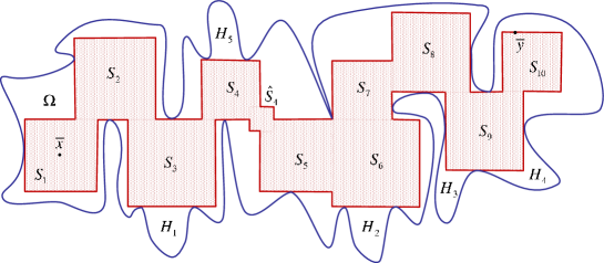
Figure 18:  

We turn to the proof of the lemma. First let us prove that

$$\partial H\cap H\neq\emptyset.$$ (4.44)

Fix a point $z_{0}\in H$. If $z_{0}\in\partial H$, then (4.44) is proven. Suppose that $z_{0}\in H^{\circ}$. We know that $\bar{x}=c_{1}$, i.e., that $\bar{x}$ is the center of $S_{1}$. Hence, $\bar{x}\in{\mathcal{W}}$, see (4.37). Let $\gamma$ be a path connecting $\bar{x}$ to $z_{0}$ in $\Omega$ so that $\gamma$ is a graph of a continuous mapping $\Gamma:[0,1]\to\Omega$ such that $\Gamma(0)=z_{0}$ and $\Gamma(1)=\bar{x}$.

Let $Y:=\{t\in[0,1]:\Gamma(t)\in{\mathcal{W}}\}$ and let $t^{\prime}:=\inf Y$. Since $\Gamma$ is a continuous mapping, $z_{0}\in H^{\circ}$ and $\bar{x}\in{\mathcal{W}}^{\circ}={\mathcal{W}}$, we conclude that $0<t^{\prime}<1$.

Let $\widetilde{z}:=\Gamma(t^{\prime}).$ Then, by definition of $t^{\prime}$, the subarc of $\gamma$ from $z_{0}$ to $\widetilde{z}$ lies in the set ${\mathcal{H}}=\Omega\setminus{\mathcal{W}}$. Since $H$ is a connected component of ${\mathcal{H}}$, $\widetilde{z}\in H$.

On the other hand, since $t^{\prime}=\inf Y\notin Y$, there exists a sequence $\{t_{m}:m=1,2,...\}\subset Y$ which converges to $t^{\prime}$ as $m\to\infty$. Let $h_{m}:=\Gamma(t_{m})$, $m=1,2,...$. Then $h_{m}\in{\mathcal{W}}$, $h_{m}\neq h_{n}$, if $m\neq n$ (because $\gamma$ is a simple path), and $h_{m}\to\widetilde{z}$ as $m\to\infty$. Hence $\widetilde{z}\in\partial H\cap H$ proving (4.44).

Prove the statements (i) and (ii). Since the parameter $k$ in representation (4.37) is finite, there exists $i\in\{1,...,k\}$ and an infinite subsequence $\{h_{m_{j}}:j=1,2,...\}$ of the sequence $\{h_{m}:m=1,2,...\}$ such that

$$h_{m_{j}}\in S_{i}\cup T_{i}~{}~{}~{}\text{for all}~{}~{}~{}j=1,2,...\,.$$

Since $h_{m}\to\widetilde{z}$ as $m\to\infty$, the subsequence $h_{m_{j}}\to\widetilde{z}$ as $j\to\infty$ proving that

$$\widetilde{z}\in S_{i}^{\operatorname{\,cl}}\cup T_{i}^{\operatorname{\,cl}}\,.$$

Recall that the set $T_{i}$ is defined by (4.35). In particular, $T_{k}=\emptyset$ and $T_{i}\subset S_{i}^{\operatorname{\,cl}}$ whenever $\#(S_{i}^{\operatorname{\,cl}}\cap S_{i+1}^{\operatorname{\,cl}})>1$. Thus, in this case $\widetilde{z}\in S_{i}^{\operatorname{\,cl}}$.

Suppose that $1\leq i<k$ and $\#(S_{i}^{\operatorname{\,cl}}\cap S_{i+1}^{\operatorname{\,cl}})=1$. In this case $\widehat{S}_{i}\neq\emptyset$ and is defined by the formula (4.19). Let us assume that $\widetilde{z}\in\widehat{S}_{i}^{\operatorname{\,cl}}$ and prove that in this case

$$H\cap S_{i}^{\operatorname{\,cl}}\neq\emptyset~{}~{}~{}\text{and}~{}~{}~{}H\cap S_{i+1}^{\operatorname{\,cl}}\neq\emptyset.$$

In fact, since $\widetilde{z}\in{\mathcal{H}}=\Omega\setminus{\mathcal{W}}$ and $S_{i},S_{i+1},\widehat{S}_{i}\subset{\mathcal{W}}$, we have $\widetilde{z}\in\partial\widehat{S}_{i}\setminus(S_{i}\cup S_{i+1})$.

We also recall that, by Lemma 4.8, see (4.24), $2\widehat{S}_{i}^{\operatorname{\,cl}}\cap S_{j}^{\operatorname{\,cl}}=\emptyset$ for every $j\in\{1,...,k\}$ such that $j\neq i,i+1$. This lemma also states that $(2\widehat{S}_{i})\cap(2\widehat{S}_{j})=\emptyset$ for every $j\in\{1,...,k\}$, $j\neq i$. Hence, by representation (4.25) (or (4.37)), we have

$$U_{i}:=(2\widehat{S}_{i})\setminus(S_{i}\cup S_{i+1}\cup\widehat{S}_{i})\subset{\mathcal{H}}=\Omega\setminus{\mathcal{W}}.$$

Clearly, there exist a point $z_{i}\in S_{i}^{\operatorname{\,cl}}\cap U_{i}$ and a path $\gamma_{1}$ in $U_{i}$ which joins $\widetilde{z}$ to $z_{i}$. Hence, $z_{i}\in H\cap S_{i}^{\operatorname{\,cl}}$. Also there exist a point $z_{i+1}\in S_{i+1}^{\operatorname{\,cl}}\cap U_{i}$ and a path $\gamma_{2}$ connecting $\widetilde{z}$ to $z_{i+1}$ in $U_{i}$, so that $z_{i+1}\in H\cap S_{i+1}^{\operatorname{\,cl}}$. See Figure 19.

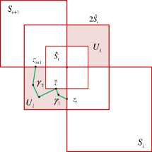
Figure 19:  

Thus we have proved that either there exists $i\in\{1,...,k\}$ such that $H\cap S_{i}^{\operatorname{\,cl}}\neq\emptyset$, or there exists $i\in\{1,...,k-1\}$ such that $H\cap S_{i}^{\operatorname{\,cl}}\neq\emptyset$ and $H\cap S_{i+1}^{\operatorname{\,cl}}\neq\emptyset$. Then, by Proposition 4.11, all the conditions of part (i) and part (ii) are satisfied. See (4.40) and (4.41).

Prove (4.42). Let $a\in H\cup S_{i}$. We have to find $\delta>0$ such that $S(a,\delta)\subset H\cup S_{i}$ provided conditions (4.40) hold.

Since $a\notin S_{j}^{\operatorname{\,cl}}$ for every $j\neq i$,

$$\delta_{1}:=\tfrac{1}{2}\operatorname{dist}(a,{\bigcup}\limits_{j\neq i}S_{j}^{\operatorname{\,cl}})>0\,.$$

As we have proved above,

$$H\cap\widehat{S}_{i}^{\operatorname{\,cl}}\neq\emptyset~{}~{}\Longrightarrow~{}~{}H\cap S_{i}^{\operatorname{\,cl}}\neq\emptyset~{}~{}~{}\text{and}~{}~{}~{}H\cap S_{i+1}^{\operatorname{\,cl}}\neq\emptyset.$$

But, by (4.40), $H\cap S_{i+1}^{\operatorname{\,cl}}=\emptyset$ so that

$$H\cap\widehat{S}_{j}^{\operatorname{\,cl}}=\emptyset~{}~{}~{}\text{for every}~{}~{}~{}j\in\{1,...,k\}.$$

Hence

$$\delta_{2}:=\tfrac{1}{2}\operatorname{dist}(a,{\bigcup}\limits_{j=1}^{k}\widehat{S}_{j}^{\operatorname{\,cl}})>0\,.$$

Let $\delta_{3}:=\tfrac{1}{2}\operatorname{dist}(a,\partial\Omega)$ and let

$$\delta:=\min\{\delta_{1},\delta_{2},\delta_{3}\}\,.$$

Then, by (4.25),

$$S(a,\delta)\cap{\mathcal{W}}=S(a,\delta)\cap S_{i}\,.$$

Hence,

$$S(a,\delta)\cap{\mathcal{H}}=S(a,\delta)\cap(\Omega\setminus{\mathcal{W}})=S(a,\delta)\setminus S_{i}\,.$$

Clearly, $S(a,\delta)\setminus S_{i}$ is a connected set so that each $z\in S(a,\delta)\setminus S_{i}$ can be joined to $a$ by a path $\gamma_{z}\subset S(a,\delta)\setminus S_{i}\subset{\mathcal{H}}$. This implies that $z$ and $a$ belong to the same connected component of ${\mathcal{H}}$, i.e., that $z\in H$.

Hence $S(a,\delta)\setminus S_{i}\subset H$ proving that $S(a,\delta)\subset S_{i}\cup H$.

Prove that $S_{i}\cup H$ is a connected set. We know that $H\cap S_{i}^{\operatorname{\,cl}}\neq\emptyset$ so that there exists $a\in H\cap S_{i}^{\operatorname{\,cl}}$.

Let $z\in H$. Since $H$ is a connected component of ${\mathcal{H}}$, this set is connected so that there exists a path $\gamma_{z}$ joining $z$ to $a$ in $H$. Then a path $\gamma=\gamma_{z}\cup[a,c_{i}]$ connects $z$ to $c_{i}$ in $S_{i}\cup H$. Thus each point $z\in S_{i}\cup H$ can be connected to $c_{i}$, the center of $S_{i}$, by a path in $S_{i}\cup H$ proving that this set is connected.

We turn to the proof of the statement (4.43), the last statement of the proposition. Let $H$ be a connected component of ${\mathcal{H}}=\Omega\setminus{\mathcal{W}}$ satisfying conditions (4.41). Let

$$V_{i}:=S_{i}\cup S_{i+1}\cup T_{i},$$ (4.45)

see (4.35), and let

$$a\in G_{i}:=H\cup V_{i}\,.$$ (4.46)

Prove the existence of $\varepsilon>0$ such that $S(a,\varepsilon)\subset G_{i}$. By (4.41),

$$\varepsilon_{1}:=\tfrac{1}{2}\operatorname{dist}(a,{\bigcup}\limits_{j\neq i,i+1}S_{j}^{\operatorname{\,cl}})>0\,.$$

In the same way as we have proved (4.41), we show that

$$H\cap\widehat{S}_{j}^{\operatorname{\,cl}}=\emptyset~{}~{}~{}\text{for every}~{}~{}~{}1\leq j\leq k,~{}j\neq i\,.$$

Hence

$$\varepsilon_{2}:=\tfrac{1}{2}\operatorname{dist}(a,{\bigcup}\limits_{j\neq i}\widehat{S}_{j}^{\operatorname{\,cl}})>0\,.$$

Finally, we put $\varepsilon_{3}:=\tfrac{1}{2}\operatorname{dist}(a,\partial\Omega)$,

$$\varepsilon_{4}:=\tfrac{1}{8}\operatorname{diam}T_{i},$$

and

$$\varepsilon:=\min\{\varepsilon_{1},\varepsilon_{2},\varepsilon_{3},\varepsilon_{4}\}\,.$$

Then, by (4.25),

$$S(a,\varepsilon)\cap{\mathcal{W}}=S(a,\varepsilon)\cap(S_{i}^{\operatorname{\,cl}}\cup S_{i+1}^{\operatorname{\,cl}}\cup\widehat{S}_{i})^{\circ}$$

so that, by (4.36),

$$S(a,\varepsilon)\cap{\mathcal{W}}=S(a,\varepsilon)\cap(S_{i}\cup S_{i+1}\cup T_{i})=S(a,\varepsilon)\cap V_{i}\,.$$

See (4.45). Hence,

$$S(a,\varepsilon)\cap{\mathcal{H}}=S(a,\varepsilon)\cap(\Omega\setminus{\mathcal{W}})=S(a,\varepsilon)\setminus V_{i}\,.$$

It can be readily seen that, by definition of $\varepsilon_{4}$, the set $S(a,\varepsilon)\setminus V_{i}$ is a connected set. Therefore every $z\in S(a,\varepsilon)\setminus V_{i}$ can be joined to $a$ by a path $\gamma_{z}\subset S(a,\varepsilon)\setminus V_{i}\subset{\mathcal{H}}$. Hence it follows that $z$ and $a$ belong to the same connected component of ${\mathcal{H}}$, i.e., that $z\in H$.

Thus we have proved that $S(a,\varepsilon)\setminus V_{i}\subset H$ so that $S(a,\varepsilon)\subset V_{i}\cup H=G_{i}$. See (4.46).

It remains to prove that the set $H\cup V_{i}$ is connected. The proof of this property is similar to that for the case (4.40). As in that case we know that $H\cap S_{i}^{\operatorname{\,cl}}\neq\emptyset$ so that, using the same approach, we show that for every $z\in H$ there exists a path $\gamma\subset H\cup V_{i}$ joining $z$ to $c_{i}$. Clearly, $V_{i}$ is a connected set and $c_{i}\in V_{i}$. Hence $c_{i}$ can be connected by a path in $H\cup V_{i}$ to an arbitrary point $z\in H\cup V_{i}$ proving the connectedness of this set.

The proof of the proposition is complete.         $\Box$

4.4. Extensions of Sobolev functions defined on “The Wide Path”. Proposition 4.12 motivates us to introduce several important geometrical objects related to “The Wide Path” ${\cal WP}_{\Omega}^{(\bar{x},\bar{y})}$. Let

$${\mathcal{C}}:=\{H:H~{}~{}\text{is a connected component of}~{}~{}{\mathcal{H}}=\Omega\setminus{\mathcal{W}}\}.$$

Given $i\in\{1,...,k\}$ we define a subfamily ${\mathcal{F}}_{i}$ of ${\mathcal{C}}$ by

$${\mathcal{F}}_{i}:=\{H\in{\mathcal{C}}:H\cap S_{i}^{\operatorname{\,cl}}\neq\emptyset\,~{}\text{and}~{}H\cap S_{j}^{\operatorname{\,cl}}=\emptyset~{}\forall~{}1\leq j\leq k,\,j\neq i\}\,.$$

C.f., part(i) of Proposition 4.12. In turn, part (ii) of this proposition motivates us to introduce a subfamily ${\mathcal{P}}_{i}$ of ${\mathcal{C}}$ as follows: given $i\in\{1,...,k-1\}$ we put

$${\mathcal{P}}_{i}:=\{H\in{\mathcal{C}}:H\cap S_{i}^{\operatorname{\,cl}}\neq\emptyset,\,H\cap S_{i+1}^{\operatorname{\,cl}}\neq\emptyset~{}\text{and}~{}H\cap S_{j}^{\operatorname{\,cl}}=\emptyset~{}\forall~{}1\leq j\leq k,\,j\neq i,i+1\}\,.$$

Note that, by Proposition 4.12, the family

$${\mathcal{F}}{\mathcal{P}}:=\{{\mathcal{F}}_{1},...,{\mathcal{F}}_{k},{\mathcal{P}}_{1},...,{\mathcal{P}}_{k-1}\}$$ (4.47)

provides a a partition of the family ${\mathcal{C}}$ of all connected components of the set ${\mathcal{H}}=\Omega\setminus{\mathcal{W}}$. In other words, ${\mathcal{F}}{\mathcal{P}}$ consists of pairwise disjoint sets which cover the family ${\mathcal{C}}$, i.e.,

$${\mathcal{C}}=\left({\bigcup}\limits_{i=1}^{k}{\mathcal{F}}_{i}\right){\bigcup}\left({\bigcup}\limits_{j=1}^{k-1}{\mathcal{P}}_{i}\right)\,.$$ (4.48)

The collection ${\mathcal{F}}{\mathcal{P}}$ enables us to introduces the following families of subsets of $\Omega$:

$$\Phi_{i}:=\left(\,{\bigcup}\limits_{H\in\,{\mathcal{F}}_{i}}H\right){\bigcup}\,S_{i},~{}~{}~{}1\leq i\leq k\,.$$ (4.49)

and

$$\Psi_{i}:=\left(\,{\bigcup}\limits_{H\in\,{\mathcal{P}}_{i}}H\right){\bigcup}\,S_{i}\,{\bigcup}\,S_{i+1}\,{\bigcup}\,T_{i},~{}~{}~{}1\leq i\leq k-1\,.$$ (4.50)

Finally we put

$$\Lambda:=\{\Phi_{1},...,\Phi_{k},\Psi_{1},...,\Psi_{k-1}\}\,.$$

The following proposition describes the main properties of the collection $\Lambda$. To its formulation given a family ${\mathcal{A}}=\{A_{\alpha}:\alpha\in I\}$ of sets in ${\bf R}^{2}$ we let $M({\mathcal{A}})$ denote its covering multiplicity, i.e., the minimal positive integer $M$ such that every point $z\in{\bf R}^{2}$ is covered by at most $M$ sets $A_{\alpha}$ from the family ${\mathcal{A}}$.

Proposition 4.13

(i) The family $\Lambda$ consists of subdomains of $\Omega$ which cover $\Omega$ with covering multiplicity $M(\Lambda)\leq 3$;

(ii) Let

$$\Lambda_{{\mathcal{H}}}:=\{\Phi_{1}\setminus{\mathcal{W}},...,\Phi_{k}\setminus{\mathcal{W}},\Psi_{1}\setminus{\mathcal{W}},...,\Psi_{k-1}\setminus{\mathcal{W}}\}.$$

Then the family $\Lambda_{{\mathcal{H}}}$ consists of pairwise disjoint sets;

(iii) For every domain $G\in\Lambda$ the set $G\cap{\mathcal{W}}$ is a Sobolev $L^{m}_{p}$-extension domain satisfying the following inequality

$$e(L^{m}_{p}(G\cap{\mathcal{W}}))\leq\,C(m,p).$$

See (1.2).

Proof. Prove (i). By Proposition 4.12, see (4.42), for each connected component $H\in{\mathcal{F}}_{i}$, $1\leq i\leq k$, the set $H\cup S_{i}$ is open and connected. In turn, by (4.43), the set $H\cup V_{i}$ where

$$V_{i}:=S_{i}\cup S_{i+1}\cup T_{i},~{}~{}~{}i=1,...k-1,$$ (4.51)

is open and connected provided $H\in{\mathcal{P}}_{i}$. Combining these facts with formulae (4.49) and (4.50), we obtain that every set $G\in\Lambda$ is a union of domains which have a non-empty intersection. Hence $G$ is a domain as well.

Recall that the family ${\mathcal{F}}{\mathcal{P}}$ defined by (4.47) is a partition of ${\mathcal{C}}$, see (4.48). Combining this property with representation (4.37) of “The Wide Path” ${\mathcal{W}}$ we conclude that

$$\Omega=\bigcup_{G\in\Lambda}\,G$$

proving that $\Lambda$ is a covering of $\Omega$.

In a similar way we prove part (ii) of the proposition. In fact, by (4.49) and (4.50),

$$\Phi_{i}\cap{\mathcal{H}}=\Phi_{i}\setminus{\mathcal{W}}={\bigcup}\limits_{H\in\,{\mathcal{F}}_{i}}H,~{}~{}~{}1\leq i\leq k,$$

and

$$\Psi_{i}\cap{\mathcal{H}}=\Psi_{i}\setminus{\mathcal{W}}={\bigcup}\limits_{H\in\,{\mathcal{P}}_{i}}H,~{}~{}~{}1\leq i\leq k-1.$$

But the collection ${\mathcal{F}}{\mathcal{P}}$ is a partition of the family ${\mathcal{C}}$, see (4.48), so that distinct members of the family $\Lambda_{{\mathcal{H}}}$ have no common points.

Prove that $M(\Lambda)\leq 3$. Let $z\in{\mathcal{H}}=\Omega\setminus{\mathcal{W}}$ and let $H\in{\mathcal{C}}$ be a connected component of ${\mathcal{H}}$ containing $z$. Since ${\mathcal{F}}{\mathcal{P}}$, see (4.47), is a partition of the family ${\mathcal{C}}$ of all connected component of ${\mathcal{H}}$, there exists a unique domain $G\in\Lambda$ which contains $z$.

This also proves that $M(\Lambda)=\max\{1,M(\Lambda_{{\mathcal{W}}})\}$ where

$$\Lambda_{{\mathcal{W}}}:=\{\Phi_{1}\cap{\mathcal{W}},...,\Phi_{k}\cap{\mathcal{W}},\Psi_{1}\cap{\mathcal{W}},...,\Psi_{k-1}\cap{\mathcal{W}}\}.$$

Note that, by definitions (4.49) and (4.50),

$$\Lambda_{{\mathcal{W}}}=\{S_{1},...,S_{k},V_{1},...,V_{k-1}\}$$

where $V_{i}$ is defined by (4.51).

It can be readily seen that $M(\Lambda_{{\mathcal{W}}})\leq 3$. In fact, suppose that $z\in S_{i}$ for some $i\in\{1,...,k\}$. Then the point $z$ can also belong to $V_{i-1}=S_{i-1}\cup S_{i}\cup T_{i-1}$ and $V_{i}=S_{i}\cup S_{i+1}\cup T_{i}$. Other members of the family $\Lambda_{{\mathcal{W}}}$ do not contain $z$. (This follows from properties of the squares $\{S_{j}\}$ presented in Lemmas 3.1, 3.2 and 3.4.) Thus in this case $z$ can be covered by at most $3$ members of the family $\Lambda_{{\mathcal{W}}}$.

Let $z\in T_{i}$ for certain $i\in\{1,...,k-1\}$, see (4.35). Clearly, in this case $z\in V_{i}$. By (4.35), if $\#(S_{i}^{\operatorname{\,cl}}\cap S_{i+1}^{\operatorname{\,cl}})>1$, i.e., if $T_{i}=(u_{i},v_{i})$, there are no exist other members of $\Lambda_{{\mathcal{W}}}$ which contain $z$. Whenever $\#(S_{i}^{\operatorname{\,cl}}\cap S_{i+1}^{\operatorname{\,cl}})=1$, i.e., $T_{i}=\widehat{S}_{i}$, only the squares $S_{i}$ and $S_{i+1}$ from the family $\Lambda_{{\mathcal{W}}}$ can contain $z$. (As in the previous case it directly follows from Lemmas 3.1, 3.2 and 3.4.) Thus in this case again the point $z$ is covered by at most $3$ members of $\Lambda_{{\mathcal{W}}}$ proving that $M(\Lambda_{{\mathcal{W}}})\leq 3$.

Hence $M(\Lambda)=\max\{1,M(\Lambda_{{\mathcal{W}}})\}\leq 3$.

Prove part (iii) of the proposition. Let $G\in\Lambda$. Then either $G=\Phi_{i}$ for some $i\in\{1,...,k\}$, or $G=\Psi_{i}$ for certain index $i\in\{1,...,k-1\}$. Hence either $G\cap{\mathcal{W}}=\Phi_{i}\cap{\mathcal{W}}=S_{i}$ or $G\cap{\mathcal{W}}=\Psi_{i}\cap{\mathcal{W}}=V_{i}$. See (4.51).

Then, by (4.36), either $V_{i}=(S_{i}^{\operatorname{\,cl}}\cup S_{i+1}^{\operatorname{\,cl}})^{\circ}$ or $V_{i}=S_{i}\cup S_{i+1}\cup\widehat{S}_{i}$. Combining this description of $V_{i}$ with the statement of Lemma 4.6 we conclude that the set $G\cap{\mathcal{W}}$ is a Sobolev extension domain such that $e(L^{m}_{p}(G\cap{\mathcal{W}}))\leq C(m,p)$.

The proposition is completely proved.         $\Box$

We turn to the proof of Theorem 1.10. Clearly, this theorem immediately follows from definition (1.2) and the following result.

Theorem 4.14

Let $p>2$ and $m\in{\bf N}$. Let $\bar{x},\bar{y}\in\Omega$ where $\Omega$ a simply connected bounded domain in ${\bf R}^{2}$. Suppose that $\Omega$ is a Sobolev $L^{m}_{p}$-extension domain.

Let ${\mathcal{W}}={\cal WP}_{\Omega}^{(\bar{x},\bar{y})}$ be a“Wide Path” joining $\bar{x}$ to $\bar{y}$ in $\Omega$ and let $f\in L^{m}_{p}({\mathcal{W}})$. Then $f$ can be extended to a function $F\in L^{m}_{p}(\Omega)$ such that

$$\|F\|_{L^{m}_{p}(\Omega)}\leq C(m,p)\,\|f\|_{L^{m}_{p}({\mathcal{W}})}\,.$$

For the proof of Theorem 4.14 we are needed the following two auxiliary results.

Proposition 4.15

([29], p. 128) If $\widetilde{{\mathcal{G}}}$ is a collection of non-empty open sets in ${\bf R}^{n}$ whose union is $U$ and if $F\in L_{1,loc}(U)$ is such that for some multi-index $\alpha$ the $\alpha$-th weak derivative of $F$ exists on each member of $\widetilde{{\mathcal{G}}}$, then $F$ has the $\alpha$-th weak derivative on $U$.

Proposition 4.16

Let $m\in{\bf N}$ and $1\leq p<\infty$ and let $V$ be a domain in ${\bf R}^{2}$.

Let ${\mathcal{G}}=\{G_{i}:i\in I\}$ be a family of domains in ${\bf R}^{2}$ satisfying the following conditions:

(i) ${\mathcal{G}}$ has finite covering multiplicity $M=M({\mathcal{G}})$;

(ii) The sets of the family $\{G_{i}\setminus V:i\in I\}$ are pairwise disjoint;

(iii) For every $G\in{\mathcal{G}}$ the set $G\cap V$ is a non-empty Sobolev $L^{m}_{p}$-extension domain. Furthermore,

$$A:=\sup_{G\in{\mathcal{G}}}\,e(L^{m}_{p}(G\cap V))<\infty.$$ (4.52)

Let

$$U:=V\,{\bigcup}\,\left\{{\bigcup}\limits_{G\in{\mathcal{G}}}G\right\}\,.$$ (4.53)

Then every function $f\in L^{m}_{p}(V)$ can be extended to a function $F\in L^{m}_{p}(U)$. Furthermore, $F$ depends on $f$ linearly and

$$\|F\|_{L^{m}_{p}(U)}\leq C\,M^{\frac{1}{p}}\,A\,\|f\|_{L^{m}_{p}(V)}$$

where $C=C(m,p)$.

Proof. Let $f\in L^{m}_{p}(V)$. We define the required extension $F$ of $f$ as follows. Let $G\in{\mathcal{G}}$. Then, by (iii), the set $G\cap{\mathcal{W}}$ is a Sobolev extension domain such that $e(L^{m}_{p}(G\cap V))\leq A$, see (4.52). Therefore there exists a function $F_{G}\in L^{m}_{p}({\bf R}^{2})$ such that

$$F_{G}|_{G\cap V}=f|_{G\cap V}$$

and

$$\|F_{G}\|_{L^{m}_{p}({\bf R}^{2})}\leq A\,\|f|_{G\cap V}\|_{L^{m}_{p}(G\cap V)}\,.$$ (4.54)

By (4.53) and by condition (ii), for each $z\in U\setminus V$ there exists a unique domain $G^{(z)}\in{\mathcal{G}}$ such that $G^{(z)}\setminus V\ni z$.

This property enables us to define the extension $F$ of $f$ by the following formula:

$$F(z):=\left\{\begin{array}[]{ll}f(z),&z\in V,\\ \\ F_{G^{(z)}}(z),&z\in U\setminus V\,.\end{array}\right.$$

Thus

$$F|_{G}=F_{G}|_{G}~{}~{}~{}\text{for every}~{}~{}G\in{\mathcal{G}}\,.$$ (4.55)

Prove that $F\in L^{m}_{p}(U)$. We know that the restriction of $F$ to $V$ and to any subdomain $G\in{\mathcal{G}}$ is a Sobolev function on $G$ so that each weak derivative of $F$ of order at most $m$ exists on $G$. Hence, by Proposition 4.15, all partial distributional derivatives of $F$ of all orders up to $m$ exist on all of $U$.

Now let us estimate the norm of $F$ in $L^{m}_{p}(U)$. We add the set $V$ to the family ${\mathcal{G}}$ and denote the new family by $\widetilde{{\mathcal{G}}}$. Clearly, by (4.53), the sets of the family $\widetilde{{\mathcal{G}}}$ cover the set $U$ so that

$$\|F\|_{L^{m}_{p}(U)}^{p} \leq C\,{{\sum}}_{|\alpha|\leq m}\,\int\limits_{U}|D^{\alpha}F|^{p}\,dz\leq C\,{{\sum}}_{|\alpha|\leq m}\,\,{{\sum}}_{G\in\widetilde{{\mathcal{G}}}}\,\int\limits_{G}|D^{\alpha}F|^{p}\,dz$$

$$= C\,{{\sum}}_{|\alpha|\leq m}\,\,{{\sum}}_{G\in\widetilde{{\mathcal{G}}}}\,\int\limits_{G}|D^{\alpha}F_{G}|^{p}\,dz=\,C\,{{\sum}}_{G\in\widetilde{{\mathcal{G}}}}\,\,{{\sum}}_{|\alpha|\leq m}\,\,\int\limits_{G}|D^{\alpha}F_{G}|^{p}\,dz\,.$$

Here $C=C(m,p)$. Hence, by (4.54),

$$\|F\|_{L^{m}_{p}(U)}^{p}\leq\,C\,A^{p}\,{{\sum}}_{G\in\widetilde{{\mathcal{G}}}}\,\,{{\sum}}_{|\alpha|\leq m}\,\,\int\limits_{G\cap V}|D^{\alpha}f|^{p}\,dz=\,C\,A^{p}\,{{\sum}}_{|\alpha|\leq m}\,\,{{\sum}}_{G\in\widetilde{{\mathcal{G}}}}\,\,\int\limits_{G\cap V}|D^{\alpha}f|^{p}\,dz\,.$$

By condition (i), covering multiplicity of the family $\{G\cap V:G\in\widetilde{{\mathcal{G}}}\}$ is bounded by $M+1$. Hence

$$\|F\|_{L^{m}_{p}(U)}^{p}\leq\,C\,A^{p}\,(M+1)\,{{\sum}}_{|\alpha|\leq m}\,\,\int\limits_{V}|D^{\alpha}f|^{p}\,dz\leq\,C\,A^{p}\,M\,\|f\|_{L^{m}_{p}(V)}^{p}\,.$$

It remains to note that, since $F_{G}$ depends on $f$ linearly, by (4.55), the function $F$ depends on $f$ linearly. The proof of the proposition is complete.         $\Box$

Proof of Theorem 4.14.

Let $\bar{x},\bar{y}\in\Omega$ and let ${\mathcal{W}}={\cal WP}_{\Omega}^{(\bar{x},\bar{y})}$ be “The Wide Path” joining $\bar{x}$ to $\bar{y}$ in $\Omega$. We suppose that $\Omega$ is a Sobolev extension domain satisfying condition (4.1) for some $\theta\geq 1$. Therefore, by Proposition 4.13, there exists a finite family

$$\Lambda:=\{\Phi_{1},...,\Phi_{k},\Psi_{1},...,\Psi_{k-1}\}$$

of subdomains of $\Omega$ satisfying conditions (i)-(iii) of this proposition. These conditions imply conditions (i)-(iii) of Proposition 4.16 provided

$$U:=\Omega,~{}~{}V:={\cal WP}_{\Omega}^{(\bar{x},\bar{y})}~{}~{}~{}\text{and}~{}~{}~{}{\mathcal{G}}:=\Lambda.$$ (4.56)

In these settings, by conditions (i) and (iii) of Proposition 4.13,

$$M:=M({\mathcal{G}})=M(\Lambda)\leq 3~{}~{}~{}\text{and}~{}~{}~{}A:=\sup\{e(L^{m}_{p}(G\cap V)):G\in{\mathcal{G}}\}\leq C(m,p).$$

Now applying Proposition 4.16 to $U,V$ and ${\mathcal{G}}$ defined by (4.56) we prove that for every $m\geq 1$, $p>2$, and every $f\in L^{m}_{p}({\mathcal{W}})$ there exists a function $F\in L^{m}_{p}(\Omega)$ linearly depending on $f$ such that

$$F|_{{\mathcal{W}}}=f~{}~{}~{}\text{and}~{}~{}~{}\|F\|_{L^{m}_{p}(\Omega)}\leq C(m,p)\,\|f\|_{L^{m}_{p}({\mathcal{W}})}.$$

The proofs of Theorem 4.14 and Theorem 1.10 are complete.         $\Box$

We finish the section with the following useful consequence of Theorem 1.10 and Theorem 4.1.

Corollary 4.17

Let $\Omega$ be a simply connected bounded domain in ${\bf R}^{2}$ satisfying condition (4.1). Then for every $\bar{x},\bar{y}\in\Omega$ and every “Wide Path” ${\cal WP}_{\Omega}^{(\bar{x},\bar{y})}$ joining $\bar{x}$ to $\bar{y}$ in $\Omega$ the following condition is satisfied: for every $a,b\in{\cal WP}_{\Omega}^{(\bar{x},\bar{y})}$ there exists a path $\gamma$ connecting $a$ to $b$ in ${\cal WP}_{\Omega}^{(\bar{x},\bar{y})}$ such that

$$\operatorname{diam}\gamma\leq\eta_{W}\|a-b\|.$$

Here $\eta_{W}$ is a positive constant satisfying the inequality $\eta_{W}\leq C(m,p)\,\theta$ where $\theta$ is the parameter from condition (4.1).

5. “The Narrow Path”

5.1. “The Narrow Path” construction algorithm. Let $\bar{x},\bar{y}\in\Omega$ and let ${\cal WP}_{\Omega}^{(\bar{x},\bar{y})}$ be “The Wide Path” joining $\bar{x}$ to $\bar{y}$ in $\Omega$ which we have constructed in the preceding section. We also recall that the domain $\Omega$ satisfies condition (4.1).

In this section we construct a “Narrow Path” described in Section 1, and present its main geometrical and Sobolev extension properties.

We begin with the following important

Lemma 5.1

Let $\varepsilon>0$. Let $K,K_{1}$ and $K_{2}$ be pairwise disjoint squares in ${\bf R}^{2}$ such that $K^{\operatorname{\,cl}}\cap K_{1}^{\operatorname{\,cl}}\neq\emptyset$, $K^{\operatorname{\,cl}}\cap K_{2}^{\operatorname{\,cl}}\neq\emptyset$, and $\#(K_{1}^{\operatorname{\,cl}}\cap K_{2}^{\operatorname{\,cl}})\leq 1$.

Then there exists a square $\widetilde{K}\subset K$ such that $\widetilde{K}^{\operatorname{\,cl}}\cap K_{1}^{\operatorname{\,cl}}\neq\emptyset$, $\widetilde{K}^{\operatorname{\,cl}}\cap K_{2}^{\operatorname{\,cl}}\neq\emptyset$ and

$$\operatorname{diam}\widetilde{K}\leq 2\operatorname{dist}(K_{1},K_{2})~{}~{}\text{whenever}~{}~{}K_{1}^{\operatorname{\,cl}}\cap K_{2}^{\operatorname{\,cl}}=\emptyset,$$

and

$$\operatorname{diam}\widetilde{K}=\varepsilon~{}~{}~{}\text{whenever}~{}~{}~{}K_{1}^{\operatorname{\,cl}}\cap K_{2}^{\operatorname{\,cl}}\neq\emptyset.$$ (5.1)

Furthermore, for every $j\in\{1,2\}$ the following is true:

$$\text{if}~{}~{}~{}\#(K_{j}^{\operatorname{\,cl}}\cap K^{\operatorname{\,cl}})>1~{}~{}~{}\text{then}~{}~{}~{}\#(K_{j}^{\operatorname{\,cl}}\cap\widetilde{K}^{\operatorname{\,cl}})>1\,.$$ (5.2)

Proof. First prove the lemma whenever $K_{1}^{\operatorname{\,cl}}\cap K_{2}^{\operatorname{\,cl}}=\emptyset$.

We begin with the following statement: for every $a,b\in K^{\operatorname{\,cl}}$ there exists a square $K_{a,b}$ such that

$$a,b\in K_{a,b}\subset K^{\operatorname{\,cl}}$$ (5.3)

and

$$\operatorname{diam}K_{a,b}=\|a-b\|\,.$$ (5.4)

(Recall that we measure distances in the uniform metric.)

Let $K=(y^{\prime},z^{\prime})\times(y^{\prime\prime},z^{\prime\prime})$. Hence, $|y^{\prime}-z^{\prime}|=|y^{\prime\prime}-z^{\prime\prime}|=\operatorname{diam}K$. Let $a=(a_{1},a_{2})$ and $b=(b_{1},b_{2})$. We may assume that

$$|a_{1}-b_{1}|\leq|a_{2}-b_{2}|=\|a-b\|\,.$$ (5.5)

Since $a,b\in K$, we have $[a_{1},b_{1}]\subset[y^{\prime},z^{\prime}]$ and

$$[a_{2},b_{2}]\subset[y^{\prime\prime},z^{\prime\prime}].$$ (5.6)

Since

$$\|a-b\|\leq\operatorname{diam}K=|y^{\prime}-z^{\prime}|,$$

by (5.5),

$$|a_{1}-b_{1}|\leq\|a-b\|\leq|y^{\prime}-z^{\prime}|.$$

Hence there exists a closed interval $[a_{1}^{\prime},b_{1}^{\prime}]$ such that

$$|a^{\prime}_{1}-b^{\prime}_{1}|=|a_{2}-b_{2}|=\|a-b\|$$

and

$$[a_{1},b_{1}]\subset[a^{\prime}_{1},b^{\prime}_{1}]\subset[y^{\prime},z^{\prime}].$$ (5.7)

Let $K_{a,b}:=(a^{\prime}_{1},b^{\prime}_{1})\times(a_{2},b_{2})$. Then, by (5.6) and (5.7), inclusions (5.3) hold. Furthermore, by (5.5),

$$\operatorname{diam}K_{a,b}=|a_{2}-b_{2}|=\|a-b\|$$

proving that $K_{a,b}$ satisfies (5.3) and (5.4).

Note that the requirements $K^{\operatorname{\,cl}}\cap K_{1}\neq\emptyset$ and $K^{\operatorname{\,cl}}\cap K_{2}\neq\emptyset$ imply the following equality:

$$\operatorname{dist}(K_{1},K_{2})=\operatorname{dist}(K_{1}^{\operatorname{\,cl}}\cap K^{\operatorname{\,cl}},K_{2}^{\operatorname{\,cl}}\cap K^{\operatorname{\,cl}})\,.$$ (5.8)

A proof of this simple geometrical fact we leave to the reader as an easy exercise.

Let $[u_{1},v_{1}]:=K_{1}^{\operatorname{\,cl}}\cap K^{\operatorname{\,cl}}$ and $[u_{2},v_{2}]:=K_{2}^{\operatorname{\,cl}}\cap K^{\operatorname{\,cl}}$. By (5.8), there exist points $a^{\prime}\in[u_{1},v_{1}]$ and $b^{\prime}\in[u_{2},v_{2}]$ such that

$$\|a^{\prime}-b^{\prime}\|=\operatorname{dist}(K_{1},K_{2}).$$

Let $a:=a^{\prime}$ whenever $u_{1}=v_{1}$, and let

$$a~{}~{}\text{be a point from}~{}~{}(u_{1},v_{1})~{}~{}\text{such that}~{}~{}\|a^{\prime}-a\|\leq\tfrac{1}{2}\operatorname{dist}(K_{1},K_{2})$$ (5.9)

whenever $u_{1}\neq v_{1}$. In a similar way we define a point $b$ by letting $b:=b^{\prime}$ whenever $u_{2}=v_{2}$, and

$$b~{}~{}\text{be a point from}~{}~{}(u_{2},v_{2})~{}~{}\text{such that}~{}~{}\|b^{\prime}-b\|\leq\tfrac{1}{2}\operatorname{dist}(K_{1},K_{2})$$ (5.10)

provided $u_{2}\neq v_{2}$.

Let $\widetilde{K}=K_{a,b}$ be the square satisfying (5.3) and (5.4). Then $a,b\in\widetilde{K}\subset K^{\operatorname{\,cl}}$ and

$$\operatorname{diam}\widetilde{K} = \|a-b\|\leq\|a-a^{\prime}\|+\|a^{\prime}-b^{\prime}\|+\|b^{\prime}-b\|$$

$$\leq \tfrac{1}{2}\operatorname{dist}(K_{1},K_{2})+\operatorname{dist}(K_{1},K_{2})+\tfrac{1}{2}\operatorname{dist}(K_{1},K_{2})=2\operatorname{dist}(K_{1},K_{2})\,.$$

Furthermore, by (5.9) and (5.10), the square $\widetilde{K}$ satisfies (5.2).

It remains to prove the statement of the lemma whenever $K_{1}^{\operatorname{\,cl}}\cap K_{2}^{\operatorname{\,cl}}$ is a singleton, see (5.1). Thus $\{a\}=K_{1}^{\operatorname{\,cl}}\cap K_{2}^{\operatorname{\,cl}}$ fore some $a\in{\bf R}^{2}$. Since $K_{1},K_{2}$ and $K$ are pairwise disjoint squares with sides parallel to the coordinate axes, the point $a$ is a common vertex of these squares. See Figure 20.

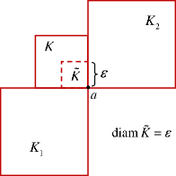
Figure 20:  

This enables us to define the square $\widetilde{K}:=K$ as follows: $\widetilde{K}$ is a (unique) subsquare of $K$ with the vertex $a$ and $\operatorname{diam}\widetilde{K}:=\varepsilon$ as it shown on Figure 20. Clearly, $\widetilde{K}$ satisfies conditions (5.1) and (5.2).

The proof of the lemma is complete.         $\Box$

We are also needed the following auxiliary result.

Lemma 5.2

Let $1\leq m\leq k-3$. Let $S_{m+1}$ be a rotation square and let $a_{m+1}$ be a rotation point associated with the square $S_{m+1}$, see Definition 4.3. (We recall that in this case $S^{\operatorname{\,cl}}_{m}\cap S^{\operatorname{\,cl}}_{m+1}\cap S^{\operatorname{\,cl}}_{m+2}=\{a_{m+1}\}$.)

Let $H$ be a square such that $H\subset S_{m+1}$, the point $a_{m+1}$ is a vertices of $H$, and

$$\operatorname{diam}H\leq\tfrac{1}{2}\min\{\operatorname{diam}S_{m},\operatorname{diam}S_{m+1},\operatorname{diam}S_{m+2}\}.$$ (5.11)

Then $H^{\operatorname{\,cl}}\cap S_{m+3}^{\operatorname{\,cl}}=\emptyset$.

Proof. First prove that

$$H^{\operatorname{\,cl}}\setminus\{a_{m+1}\}\subset S_{m}\cup S_{m+1}\cup S_{m+2}.$$ (5.12)

In fact, by (5.11),

$$H^{\operatorname{\,cl}}\setminus\{a_{m+1}\}=H\cup((H^{\operatorname{\,cl}}\cap S_{m}^{\operatorname{\,cl}})\setminus\{a_{m+1}\})\cup((H^{\operatorname{\,cl}}\cap S_{m+2}^{\operatorname{\,cl}})\setminus\{a_{m+1}\}).$$

We know that $H\subset S_{m+1}$. Recall that

$$[u_{m},v_{m}]=S_{m}^{\operatorname{\,cl}}\cap S_{m+1}^{\operatorname{\,cl}}~{}~{}~{}\text{and}~{}~{}~{}[u_{m+1},v_{m+1}]=S_{m+1}^{\operatorname{\,cl}}\cap S_{m+2}^{\operatorname{\,cl}}\,.$$

See (4.2). (We can assume that $u_{m}=u_{m+1}=a_{m+1}$.) We also know that $T_{m}=(u_{m},v_{m})\subset\Omega$ and $T_{m+1}=(u_{m+1},v_{m+1})\subset\Omega$, see (4.35) and (4.37). These properties and inequality (5.11) imply the following:

$$(H^{\operatorname{\,cl}}\cap S_{m}^{\operatorname{\,cl}})\setminus\{a_{m+1}\}\subset(u_{m},v_{m})\subset\Omega~{}~{}\text{and}~{}~{}(H^{\operatorname{\,cl}}\cap S_{m+2}^{\operatorname{\,cl}})\setminus\{a_{m+1}\}\subset(u_{m+1},v_{m+1})\subset\Omega,$$

proving (5.12).

By (5.12) an Lemma 3.2, $(H^{\operatorname{\,cl}}\setminus\{a_{m+1}\})\cap S_{m+3}^{\operatorname{\,cl}}=\emptyset$. On the other hand, $a_{m+1}\in S_{m}^{\operatorname{\,cl}}$ and, by (4.4), $S_{m}^{\operatorname{\,cl}}\cap S_{m+3}^{\operatorname{\,cl}}=\emptyset$. Hence $a_{m+1}\notin S_{m+3}^{\operatorname{\,cl}}$. Thus $H^{\operatorname{\,cl}}\cap S_{m+3}^{\operatorname{\,cl}}=\emptyset$, and the proof of the lemma is complete.         $\Box$

We turn to constructing “The Narrow Path”. Let ${\mathcal{S}}_{\Omega}(\bar{x},\bar{y})=\{S_{1},S_{2},...,S_{k}\}$ be the family of squares constructed in “The Wide Path Theorem” 1.9.

Proposition 5.3

Let $k>2$. There exists a family

$${\mathcal{Q}}_{\Omega}(\bar{x},\bar{y})=\{Q_{1},Q_{2},...,Q_{k}\}$$

of pairwise disjoint squares such that:

(1). $Q_{1}=S_{1}$, $Q_{k}=S_{k}$, and $Q_{i}\subset S_{i}$ for every $i,1\leq i\leq k$. Furthermore, $\bar{x}$ is the center of $Q_{1}$. In turn, $\bar{y}\in Q_{k}^{\operatorname{\,cl}}$ and $\operatorname{dist}(\bar{y},Q_{k-1})=\operatorname{diam}Q_{k}$ ;

(2). $Q_{i}^{\operatorname{\,cl}}\cap Q_{i+1}^{\operatorname{\,cl}}\neq\emptyset$ for every $i\in\{1,...,k-1\}$, and $\#(Q_{i}^{\operatorname{\,cl}}\cap Q_{i+2}^{\operatorname{\,cl}})\leq 1$ for every $i\in\{1,...,k-2\}$. Furthermore,

$$\,Q_{i}^{\operatorname{\,cl}}\cap Q_{j}^{\operatorname{\,cl}}=\emptyset~{}~{}~{}\text{for all}~{}~{}~{}i,j\in\{1,...,k\},~{}|i-j|>2\,;$$

(3). If $\#(S_{i}^{\operatorname{\,cl}}\cap S_{i+1}^{\operatorname{\,cl}})>1$, then $\#(Q_{i}^{\operatorname{\,cl}}\cap Q_{i+1}^{\operatorname{\,cl}})>1$. In turn, if $\#(S_{i}^{\operatorname{\,cl}}\cap S_{i+1}^{\operatorname{\,cl}})=1$, then $\#(Q_{i}^{\operatorname{\,cl}}\cap Q_{i+1}^{\operatorname{\,cl}})=1$ as well;

(4). Let $1\leq i\leq k-2$. Then

$$\operatorname{diam}Q_{i+1}\leq 2\operatorname{dist}(Q_{i},Q_{i+2})~{}~{}~{}\text{if}~{}~{}~{}Q_{i}^{\operatorname{\,cl}}\cap S_{i+2}^{\operatorname{\,cl}}=\emptyset,$$ (5.13)

and

$$\operatorname{diam}Q_{i+1}\leq\,\tfrac{1}{4}\min\{\operatorname{diam}Q_{i},\operatorname{diam}Q_{i+2}\}~{}~{}~{}\text{if}~{}~{}~{}Q_{i}^{\operatorname{\,cl}}\cap S_{i+2}^{\operatorname{\,cl}}\neq\emptyset\,;$$ (5.14)

(5). If $Q_{i}^{\operatorname{\,cl}}\cap S_{i+2}^{\operatorname{\,cl}}\neq\emptyset$ then $Q_{i+1}^{\operatorname{\,cl}}\cap S_{i+3}^{\operatorname{\,cl}}=\emptyset$, $1\leq i\leq k-3$.

See Figure 2.

Proof. We obtain the family ${\mathcal{Q}}_{\Omega}(\bar{x},\bar{y})$ as a result of a $k$ step inductive procedure based on Lemma 5.1. This procedure depends on a certain parameter $\varepsilon_{0}>0$ which we define as follows. Let

$$J:=\{m\in\{1,...,k-3\}:S_{m}^{\operatorname{\,cl}}\cap S_{m+1}^{\operatorname{\,cl}}\cap S_{m+2}^{\operatorname{\,cl}}\neq\emptyset\}.$$

Thus for every $m\in J$ the square $S_{m+1}$ is a rotation square, see Definition 4.3. Let $a_{m+1}$ be the rotation point associated with $S_{m+1}$ so that

$$\{a_{m+1}\}=S^{\operatorname{\,cl}}_{m}\cap S^{\operatorname{\,cl}}_{m+1}\cap S^{\operatorname{\,cl}}_{m+2}.$$

We let $H_{m}$ denote a subsquare of $S_{m+1}$ such that $a_{m+1}$ is a vertices of $H_{m}$ and

$$\operatorname{diam}H_{m}:=\tfrac{1}{4}\min\{\operatorname{diam}S_{m},\operatorname{diam}S_{m+1},\operatorname{diam}S_{m+2}\}.$$ (5.15)

Let

$$\varepsilon_{0}:=\tfrac{1}{4}\min\{\operatorname{dist}(H_{m},S_{m+3}):m\in J\}.$$ (5.16)

By Lemma 5.2, $\operatorname{dist}(H_{m},S_{m+3})>0$ for every $m\in J$ so that $\varepsilon_{0}>0$.

We are in a position to define the family of squares ${\mathcal{Q}}_{\Omega}(\bar{x},\bar{y})$. At the first step of our inductive procedure we put $Q_{1}:=S_{1}$ and turn to the second step. We know that

$$Q_{1}^{\operatorname{\,cl}}\cap S_{2}^{\operatorname{\,cl}}\neq\emptyset,~{}~{}S_{2}^{\operatorname{\,cl}}\cap S_{3}^{\operatorname{\,cl}}\neq\emptyset~{}~{}~{}\text{and}~{}~{}~{}\#(Q_{1}^{\operatorname{\,cl}}\cap S_{3}^{\operatorname{\,cl}})\leq 1,$$

see part (ii) of Lemma 4.2. We put

$$\varepsilon:=\tfrac{1}{4}\min\{\operatorname{diam}Q_{1},\operatorname{diam}S_{2},\operatorname{diam}S_{3},\varepsilon_{0}\}$$

and apply Lemma 5.1 to $\varepsilon$ and pairwise disjoint squares $K_{1}:=Q_{1},K:=S_{2},$ and $K_{3}:=S_{3}$. By this lemma, there exists a square $\widetilde{K}$ such that $\widetilde{K}\subset S_{2}$,

$$\widetilde{K}^{\operatorname{\,cl}}\cap Q_{1}^{\operatorname{\,cl}}\neq\emptyset~{}~{}~{}\text{and}~{}~{}~{}\widetilde{K}^{\operatorname{\,cl}}\cap S_{3}^{\operatorname{\,cl}}\neq\emptyset.$$

Furthermore,

$$\operatorname{diam}\widetilde{K}\leq 2\operatorname{dist}(Q_{1},S_{3})~{}~{}~{}\text{if}~{}~{}~{}Q_{1}^{\operatorname{\,cl}}\cap S_{3}^{\operatorname{\,cl}}=\emptyset,$$

and

$$\operatorname{diam}\widetilde{K}=\varepsilon~{}~{}~{}\text{if}~{}~{}~{}Q_{1}^{\operatorname{\,cl}}\cap S_{3}^{\operatorname{\,cl}}\neq\emptyset.$$

In addition, if $\#(Q_{1}^{\operatorname{\,cl}}\cap S_{2}^{\operatorname{\,cl}})>1$, then $\#(Q_{1}^{\operatorname{\,cl}}\cap\widetilde{K}^{\operatorname{\,cl}})>1$, and if $\#(Q_{1}^{\operatorname{\,cl}}\cap S_{2}^{\operatorname{\,cl}})=1$, then $\#(Q_{1}^{\operatorname{\,cl}}\cap\widetilde{K}^{\operatorname{\,cl}})=1$ as well. The same is true for the squares $S_{3}$ and $S_{2}$, i.e.,

$$\text{if}~{}~{}~{}\#(S_{2}^{\operatorname{\,cl}}\cap S_{3}^{\operatorname{\,cl}})>1~{}~{}\text{then}~{}~{}\#(\widetilde{K}^{\operatorname{\,cl}}\cap S_{3}^{\operatorname{\,cl}})>1,$$

and

$$\text{if}~{}~{}~{}\#(S_{2}^{\operatorname{\,cl}}\cap S_{3}^{\operatorname{\,cl}})=1~{}~{}\text{then}~{}~{}\#(\widetilde{K}^{\operatorname{\,cl}}\cap S_{3}^{\operatorname{\,cl}})=1.$$

We put $Q_{2}:=\widetilde{K}$ and turn to the third step. We know that $Q_{2}^{\operatorname{\,cl}}\cap S_{3}^{\operatorname{\,cl}}\neq\emptyset$, $S_{3}^{\operatorname{\,cl}}\cap S_{4}^{\operatorname{\,cl}}\neq\emptyset$ and $\#(Q_{2}^{\operatorname{\,cl}}\cap S_{4}^{\operatorname{\,cl}})\leq 1$ (because $Q_{2}\subset S_{2}$ and, by part (ii) of Lemma 4.2, $\#(S_{2}^{\operatorname{\,cl}}\cap S_{4}^{\operatorname{\,cl}})\leq 1$). This enables us to apply Lemma 5.1 to

$$\varepsilon:=\tfrac{1}{4}\min\{\operatorname{diam}Q_{2},\operatorname{diam}S_{3},\operatorname{diam}S_{4},\varepsilon_{0}\}$$

and pairwise disjoint squares $K_{1}:=Q_{2},K:=S_{3}$ and $K_{3}:=S_{4}$, and in this way to obtain a square $Q_{3}$, etc.

In a similar way we turn from the $m$-th step of this algorithm to its $(m+1)$-th step provided $1\leq m<k-1$. After $m$ steps of this procedure we obtain a collection of squares $\{Q_{1},Q_{2},...,Q_{m}\}$. We know that $Q_{m}\subset S_{m}$, $\,Q_{m}^{\operatorname{\,cl}}\cap S_{m+1}^{\operatorname{\,cl}}\neq\emptyset$, $\,S_{m+1}^{\operatorname{\,cl}}\cap S_{m+2}^{\operatorname{\,cl}}\neq\emptyset$ and $\,\#(Q_{m}^{\operatorname{\,cl}}\cap S_{m+2}^{\operatorname{\,cl}})\leq 1$ (because $Q_{m}\subset S_{m}$ and, by part (ii) of Lemma 4.2, $\#(S_{m}^{\operatorname{\,cl}}\cap S_{m+2}^{\operatorname{\,cl}})\leq 1)$. We put

$$\varepsilon:=\tfrac{1}{4}\min\{\operatorname{diam}Q_{m},\operatorname{diam}S_{m+1},\operatorname{diam}S_{m+2},\varepsilon_{0}\},$$

$K_{1}:=Q_{m},K:=S_{m+1}$ and $K_{2}:=S_{m+2}$. Clearly, $K_{1},K,K_{2}$ is a triple of pairwise disjoint squares satisfying the hypothesis of Lemma 5.1.

By this lemma, there exists a square $Q_{m+1}=\widetilde{K}$ such that $Q_{m+1}\subset S_{m+1}$,

$$Q_{m}^{\operatorname{\,cl}}\cap Q_{m+1}^{\operatorname{\,cl}}\neq\emptyset~{}~{}~{}\text{and}~{}~{}~{}Q_{m+1}^{\operatorname{\,cl}}\cap S_{m+2}^{\operatorname{\,cl}}\neq\emptyset.$$ (5.17)

Furthermore,

$$\operatorname{diam}Q_{m+1}\leq 2\operatorname{dist}(Q_{m},S_{m+2})~{}~{}~{}\text{whenever}~{}~{}~{}Q_{m}^{\operatorname{\,cl}}\cap S_{m+2}^{\operatorname{\,cl}}=\emptyset.$$ (5.18)

See Figure 21.

Figure 21:  

Now let

$$Q_{m}^{\operatorname{\,cl}}\cap S_{m+2}^{\operatorname{\,cl}}\neq\emptyset.$$ (5.19)

Since $Q_{m}\subset S_{m}$, we have $S_{m}^{\operatorname{\,cl}}\cap S_{m+2}^{\operatorname{\,cl}}\neq\emptyset$, so that the square $S_{m+1}$ is a rotation square of “The Wide Path” ${\mathcal{W}}$, see Definition 4.3. We know that in this case the intersection $S_{m}\cap S_{m+1}\cap S_{m+2}$ is the rotation point $\{a_{m+1}\}$ associated with the rotation square $S_{m+1}$.

By Lemma 5.1, in this case

$$\operatorname{diam}Q_{m+1}=\varepsilon=\,\tfrac{1}{4}\min\{\operatorname{diam}Q_{m},\operatorname{diam}S_{m+1},\operatorname{diam}S_{m+2},\varepsilon_{0}\}.$$ (5.20)

In addition, by (5.2),

$$\text{if}~{}~{}~{}\#(Q_{m}^{\operatorname{\,cl}}\cap S_{m+1}^{\operatorname{\,cl}})>1~{}~{}\text{then}~{}~{}\#(Q_{m}^{\operatorname{\,cl}}\cap Q_{m+1}^{\operatorname{\,cl}})>1,$$ (5.21)

and

$$\text{if}~{}~{}~{}\#(S_{m+1}^{\operatorname{\,cl}}\cap S_{m+2}^{\operatorname{\,cl}})>1~{}~{}\text{then}~{}~{}\#(Q_{m+1}^{\operatorname{\,cl}}\cap S_{m+2}^{\operatorname{\,cl}})>1.$$ (5.22)

See Figure 22.

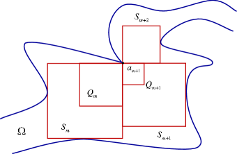
Figure 22:  

After $(k-1)$ steps of this algorithm we obtain a family of squares $\{Q_{1},...,Q_{k-1}\}$. Finally, at the last step of this procedure we put $Q_{k}:=S_{k}$ and stop.

Let us prove that the obtained family $\{Q_{1},...,Q_{k}\}$ of squares possesses properties (1)-(5) of the proposition.

Since $Q_{1}=S_{1}$, $Q_{k}=S_{k}$ and $Q_{m+1}\subset S_{m+1}$, the first part of property (1) holds. The second and third parts follow from part (a) of Lemma 3.1. Property (2) of the proposition follows from (5.17) and part (ii) of Lemma 4.2. Property (3) directly follows from properties (5.21) and (5.22) and the inclusion $Q_{i}\subset S_{i}$, $1\leq i\leq k$.

Prove property (4). Suppose that $Q_{m}^{\operatorname{\,cl}}\cap S_{m+2}^{\operatorname{\,cl}}=\emptyset$. Since $Q_{m+2}\subset S_{m+2}$, by (5.18),

$$\operatorname{diam}Q_{m+1}\leq 2\operatorname{dist}(Q_{m},S_{m+2})\leq 2\operatorname{dist}(Q_{m},Q_{m+2})$$

proving (5.13).

Now prove (5.14) whenever $Q_{m}^{\operatorname{\,cl}}\cap S_{m+2}^{\operatorname{\,cl}}\neq\emptyset$, i.e., (5.19) holds. In this case $Q_{m+1}$ is a subsquare of $S_{m+1}$, the rotation point $a_{m+1}$ is a vertices of $Q_{m+1}$ and its diameter is given by (5.20). See Figure 22.

Comparing $Q_{m+1}$ with the square $H_{m+1}$ defined at the beginning of the proof (see (5.15)) we conclude that $Q_{m+1}\subset H_{m+1}$. Note that, by (5.16) and (5.20),

$$\operatorname{diam}Q_{m+1}\leq\varepsilon_{0}\leq\tfrac{1}{4}\operatorname{dist}(H_{m},S_{m+3}).$$

On the other hand, we know that $Q^{\operatorname{\,cl}}_{m+2}\cap Q^{\operatorname{\,cl}}_{m+1}\neq\emptyset$ and $Q^{\operatorname{\,cl}}_{m+2}\cap S^{\operatorname{\,cl}}_{m+3}\neq\emptyset$ so that

$$\operatorname{diam}Q_{m+2}\geq\operatorname{dist}(Q_{m+1},S_{m+3})\geq\operatorname{dist}(H_{m+1},S_{m+3})\geq 4\varepsilon_{0}.$$

Hence $\operatorname{diam}Q_{m+1}\leq\frac{1}{4}\operatorname{diam}Q_{m+2}$.

In addition, by (5.20), $\operatorname{diam}Q_{m+1}\leq\frac{1}{4}\operatorname{diam}Q_{m}$ proving (5.14) and property (4) of the proposition.

Prove property (5). Suppose that (5.19) holds so that $a_{m+1}$ is a rotation point associated with the rotation square $S_{m+1}$. See Figure 22.

Let $H:=Q_{m+1}$. Then $H\subset S_{m+1}$, the point $a_{m+1}$ is a vertices of $H$, and, by (5.20), inequality (5.11) of Lemma 5.2 is satisfied. By this lemma, $H^{\operatorname{\,cl}}\cap S_{m+3}^{\operatorname{\,cl}}=\emptyset$ proving that $Q_{m+1}^{\operatorname{\,cl}}\cap S_{m+3}^{\operatorname{\,cl}}=\emptyset$. This implies property (5).

The proof of the proposition is complete.         $\Box$

5.2. Main geometrical properties of “The Narrow Path”. We recall that “The Narrow Path” ${\cal NP}_{\Omega}^{(\bar{x},\bar{y})}$ joining $\bar{x}$ to $\bar{y}$ in $\Omega$ is defined by formula (1.20):

$${\cal NP}_{\Omega}^{(\bar{x},\bar{y})}:=\left(\,\bigcup_{i=1}^{k}\left(\,Q_{i}^{\operatorname{\,cl}}\,{\bigcup}\,\widehat{S}_{i}\,\right)\right)^{\circ}.$$

Recall that $\{\widehat{S}_{1},...,\widehat{S}_{k}\}$ is the family of sets (more specifically, squares or empty sets) introduced in Definition 4.7.

Let us present several useful geometrical properties of “The Narrow Path” which we will use later on in the study of the extension properties of ${\cal NP}_{\Omega}^{(\bar{x},\bar{y})}$ and differential properties of the “rapidly growing” functions.

Lemma 5.4

(i). $\widehat{S}_{i}=\emptyset$ whenever $i=k$ or $\#(Q_{i}^{\operatorname{\,cl}}\cap Q_{i+1}^{\operatorname{\,cl}})>1$, and

$$\widehat{S}_{i}=S(w_{i},\hat{\delta})~{}~{}~{}\text{if}~{}~{}~{}\#(Q_{i}^{\operatorname{\,cl}}\cap Q_{i+1}^{\operatorname{\,cl}})=1.$$

Here $\{w_{i}\}=S_{i}^{\operatorname{\,cl}}\cap S_{i+1}^{\operatorname{\,cl}}$, see (4.20), and $\hat{\delta}$ is the number defined by (4.21).

(ii). $\{\widehat{S}_{1},...,\widehat{S}_{k}\}$ is a family of pairwise disjoint subsets of $\Omega$ such that

$$(\widehat{S}_{i}^{\operatorname{\,cl}})\cap Q_{j}^{\operatorname{\,cl}}=\emptyset~{}~{}\text{for every}~{}~{}1\leq i,j\leq k,\,j\neq i,i+1.$$ (5.23)

(iii). $\operatorname{diam}\widehat{S}_{i}\leq\frac{1}{4}\,\min\{\operatorname{diam}Q_{i},\operatorname{diam}Q_{i+1}\}$ for every $i,1\leq i\leq k-1$.

Proof. By part (3) of Proposition 5.3,

$$\#(Q_{i}^{\operatorname{\,cl}}\cap Q_{i+1}^{\operatorname{\,cl}})=1~{}~{}~{}\text{if and only if}~{}~{}~{}\#(S_{i}^{\operatorname{\,cl}}\cap S_{i+1}^{\operatorname{\,cl}})=1.$$

This property, Definition 4.7 (see(4.18) and (4.19)) imply part (i) of the lemma.

Prove (ii). By Lemma 4.8, the sets of the family $\{2\widehat{S}_{i}:1=1,...,k\}$ are pairwise disjoint subsets of $\Omega$ so that the family $\{\widehat{S}_{i}:1=1,...,k\}$ consists of pairwise disjoint subsets of $\Omega$ as well. This property, (4.24) and the inclusion $Q_{i}\subset S_{i}$ immediately imply the statement (5.23) proving (ii).

Prove (iii). Suppose that $\widehat{S}_{i}\neq\emptyset$, i.e., by part (i) of the present lemma, $Q_{i}^{\operatorname{\,cl}}\cap Q_{i+1}^{\operatorname{\,cl}}=\{w_{i}\}$. (Recall that $w_{i}$ is the center of the square $\widehat{S}_{i}$.) Thus $w_{i}\in Q_{i}^{\operatorname{\,cl}}$.

If $i=1$ then, by part (1) of Proposition 5.3, $Q_{1}=S_{1}$. In turn, by (4.21),

$$\hat{\delta}\leq\tfrac{1}{8}\,\hat{\delta}_{2}=\min\{\operatorname{diam}S_{j}:1\leq j\leq k\}$$

so that

$$\operatorname{diam}\widehat{S}_{i}=2\,\hat{\delta}\leq\tfrac{1}{4}\operatorname{diam}S_{j}~{}~{}~{}\text{for every}~{}~{}~{}1\leq i,j\leq k.$$ (5.24)

In particular, $\operatorname{diam}\widehat{S}_{1}\leq\tfrac{1}{4}\operatorname{diam}S_{1}=\tfrac{1}{4}\operatorname{diam}Q_{1}$.

Now let $i>1$. Since $Q_{i-1}^{\operatorname{\,cl}}\cap Q_{i}^{\operatorname{\,cl}}\neq\emptyset$ and $Q_{i-1}\subset S_{i-1}$, we have $\operatorname{dist}(w_{i},S_{i-1})\leq\operatorname{diam}Q_{i}$. But, by (4.22) and (4.21),

$$\operatorname{diam}\widehat{S}_{i}=2\hat{\delta}\leq 2\cdot\tfrac{1}{8}\,\hat{\delta}_{3}\leq\tfrac{1}{4}\operatorname{dist}(w_{i},S_{i-1})\leq\tfrac{1}{4}\operatorname{diam}Q_{i}.$$

In the same way we prove that $\operatorname{diam}\widehat{S}_{i}\leq\tfrac{1}{4}\operatorname{diam}Q_{i+1}$. In fact, let $i<k-1$. Since $Q_{i+1}^{\operatorname{\,cl}}\cap S_{i+2}^{\operatorname{\,cl}}\neq\emptyset$, we have $\operatorname{dist}(w_{i},S_{i+1})\leq\operatorname{diam}Q_{i+1}$. Hence,

$$\operatorname{diam}\widehat{S}_{i}=2\hat{\delta}\leq 2\cdot\tfrac{1}{8}\,\hat{\delta}_{3}\leq\tfrac{1}{4}\operatorname{dist}(w_{i},S_{i+1})\leq\tfrac{1}{4}\operatorname{diam}Q_{i+1}.$$

If $i=k-1$ then, by part (1) of Proposition 5.3, $Q_{i+1}=Q_{k}=S_{k}$ so that, by (5.24), $\operatorname{diam}\widehat{S}_{k-1}\leq\tfrac{1}{4}\operatorname{diam}S_{k}=\tfrac{1}{4}\operatorname{diam}Q_{k}$ proving part (iii) and the lemma.         $\Box$

The next proposition is an analog of Proposition 4.9 for “The Narrow Path”. Its proof literally follows the scheme of the proof of Proposition 4.9; we leave the details for the interested reader.

Proposition 5.5

“The Narrow Path” ${\mathcal{N}}:={\cal NP}_{\Omega}^{(\bar{x},\bar{y})}$ is an open connected subset of the domain $\Omega$ which has the following representation:

$${\mathcal{N}}=\bigcup_{i=1}^{k-1}\left(\,Q_{i}^{\operatorname{\,cl}}\,{\bigcup}\,Q_{i+1}^{\operatorname{\,cl}}\,{\bigcup}\,\widehat{S}_{i}\,\right)^{\circ}\,.$$ (5.25)

Let $Q_{i}$ and $Q_{i+1}$, $1\leq i<k$, be two subsequent squares from “The Narrow Path” such that $\#(Q_{i}^{\operatorname{\,cl}}\cap Q_{i+1}^{\operatorname{\,cl}})>1$. Since $Q_{i}$ and $Q_{i+1}$ are touching squares, intersection of their closures is a line segment. We denote the ends of this segment by $s_{i}$ and $t_{i}$. Thus

$$[s_{i},t_{i}]:=Q_{i}^{\operatorname{\,cl}}\cap Q_{i+1}^{\operatorname{\,cl}}~{}~{}~{}\text{whenever}~{}~{}~{}\#(Q_{i}^{\operatorname{\,cl}}\cap Q_{i+1}^{\operatorname{\,cl}})>1,$$ (5.26)

so that in this case

$$(Q_{i}^{\operatorname{\,cl}}\cup Q_{i+1}^{\operatorname{\,cl}})^{\circ}=Q_{i}\cup Q_{i+1}\cup(s_{i},t_{i}).$$ (5.27)

Let $1\leq i<k$ and let

$$Y_{i}:=\left\{\begin{array}[]{ll}\widehat{S}_{i},&~{}~{}\text{if}~{}~{}\#(Q_{i}^{\operatorname{\,cl}}\cap Q_{i+1}^{\operatorname{\,cl}})=1,\\ \\ (s_{i},t_{i}),&~{}~{}\text{if}~{}~{}\#(Q_{i}^{\operatorname{\,cl}}\cap Q_{i+1}^{\operatorname{\,cl}})>1.\end{array}\right.$$ (5.31)

We also put $Y_{k}:=\emptyset$.

Then, by (5.27) and by definition of $\widehat{S}_{i}$, see (4.19),

$$\left(\,Q_{i}^{\operatorname{\,cl}}\,{\bigcup}\,Q_{i+1}^{\operatorname{\,cl}}\,{\bigcup}\,\widehat{S}_{i}\,\right)^{\circ}=Q_{i}\,{\bigcup}\,Q_{i+1}\,{\bigcup}\,Y_{i}\,.$$ (5.32)

Combining this equality with (5.25) we obtain the following representation of “The Narrow Path”:

$${\mathcal{N}}={\cal NP}_{\Omega}^{(\bar{x},\bar{y})}={\bigcup}\limits_{i=1}^{k}\left(Q_{i}\,{\bigcup}\,Y_{i}\right)\,.$$ (5.33)

In the next two lemmas we present additional geometrical properties of ”The Narrow Path”.

Lemma 5.6

(i) Let $1\leq i\leq k-2$ and let $Q_{i}^{\operatorname{\,cl}}\cap S_{i+2}^{\operatorname{\,cl}}=\emptyset$. Then

$$\operatorname{diam}Q_{i+1}\leq 4\operatorname{dist}(Y_{i},Y_{i+1}).$$ (5.34)

Furthermore,

$$\operatorname{diam}Q_{1}\leq 4\operatorname{dist}(\bar{x},Y_{1})~{}~{}~{}\text{and}~{}~{}~{}\operatorname{diam}Q_{k}\leq 4\operatorname{dist}(\bar{y},Y_{k-1}).$$ (5.35)

Proof. (i) Suppose that $\#(Q_{i}^{\operatorname{\,cl}}\cap Q_{i+1}^{\operatorname{\,cl}})=1$ so that $Y_{i}=\widehat{S}_{i}$. See Definition 4.7. Consider two cases.

The first case: $\#(Q_{i+1}^{\operatorname{\,cl}}\cap Q_{i+2}^{\operatorname{\,cl}})=1$. In this case $Y_{i+1}=\widehat{S}_{i+1}$. Recall that the center of the square $\widehat{S}_{i+1}$, the point $w_{i+1}$, is a common vertex of the squares $Q_{i+1}^{\operatorname{\,cl}}$ and $Q_{i+2}^{\operatorname{\,cl}}$. Furthermore, since $\widehat{S}_{i}\cap\widehat{S}_{i+1}=\emptyset$, we have $w_{i}\neq w_{i+1}$.

Since $w_{i}$ is a vertex of $Q_{i+1}^{\operatorname{\,cl}}$ as well, we conclude that

$$\|w_{i}-w_{i+1}\|=\operatorname{diam}Q_{i+1}\,.$$ (5.36)

By part (iii) of Lemma 5.4,

$$\operatorname{diam}\widehat{S}_{i},\,\operatorname{diam}\widehat{S}_{i+1}\leq\tfrac{1}{4}\operatorname{diam}Q_{i+1}\,.$$

Combining this inequality with (5.36), we obtain that

$$\operatorname{dist}(Y_{i},Y_{i+1})=\operatorname{dist}(\widehat{S}_{i},\widehat{S}_{i+1})\geq\tfrac{1}{2}\operatorname{diam}Q_{i+1}\,.$$

In the same fashion, basing on property (1) of Lemma 5.3, we prove inequalities (5.35).

The second case: $\#(Q_{i+1}^{\operatorname{\,cl}}\cap Q_{i+2}^{\operatorname{\,cl}})>1$. In this case $Y_{i+1}=(s_{i+1},t_{i+1})\subset Q_{i+1}^{\operatorname{\,cl}}\cap Q_{i+2}^{\operatorname{\,cl}}$. Since $Q_{i}^{\operatorname{\,cl}}\cap S_{i+2}^{\operatorname{\,cl}}=\emptyset$, by (5.13),

$$\operatorname{diam}Q_{i+1}\leq 2\operatorname{dist}(Q_{i},Q_{i+2})\leq 2\operatorname{dist}(w_{i},Y_{i+1})\,.$$

On the other hand, by part (iii) of Lemma 5.4, $\operatorname{diam}\widehat{S}_{i}\leq\tfrac{1}{4}\operatorname{diam}Q_{i+1}$. Therefore, for each $z\in\widehat{S}_{i}$ we have

$$\operatorname{dist}(Y_{i+1},z)\geq\operatorname{dist}(Y_{i+1},w_{i})-\|z-w_{i}\|\geq\tfrac{1}{2}\operatorname{diam}Q_{i+1}-\tfrac{1}{4}\operatorname{diam}Q_{i+1}=\tfrac{1}{4}\operatorname{diam}Q_{i+1}$$

proving (5.34) in the case under consideration.

Let now $\#(Q_{i}^{\operatorname{\,cl}}\cap Q_{i+1}^{\operatorname{\,cl}})>1$ and $\#(Q_{i+1}^{\operatorname{\,cl}}\cap Q_{i+2}^{\operatorname{\,cl}})>1$. In this case $Y_{i}=(s_{i},t_{i})\subset Q_{i}^{\operatorname{\,cl}}$ and $Y_{i+1}=(s_{i+1},t_{i+1})\subset Q_{i+2}^{\operatorname{\,cl}}$. Hence, by (5.13),

$$\operatorname{dist}(\widehat{S}_{i},\widehat{S}_{i+1})=\operatorname{dist}(Y_{i},Y_{i+1})\geq\operatorname{dist}(Q_{i},Q_{i+2})\geq\tfrac{1}{2}\operatorname{diam}Q_{i+1}.$$

Consider the remaining case where $\#(Q_{i}^{\operatorname{\,cl}}\cap Q_{i+1}^{\operatorname{\,cl}})>1$ and $\#(Q_{i+1}^{\operatorname{\,cl}}\cap Q_{i+2}^{\operatorname{\,cl}})=1$, i.e., $Y_{i}=(s_{i},t_{i})\subset Q_{i}^{\operatorname{\,cl}}$ and $Y_{i+1}=\widehat{S}_{i+1}$.

Recall that $\widehat{S}_{i+1}=S(w_{i+1},\hat{\delta})$ where $\{w_{i+1}\}=Q_{i+1}^{\operatorname{\,cl}}\cap Q_{i+2}^{\operatorname{\,cl}}$ and $\hat{\delta}$ is defined by (4.21). In particular, by $\hat{\delta}\leq\tfrac{1}{8}\,\hat{\delta}_{3}\leq\tfrac{1}{8}\operatorname{dist}(w_{i+1},S_{i})$. But $w_{i+1}\in Q^{\operatorname{\,cl}}_{i+1}$ and $Q_{i+1}^{\operatorname{\,cl}}\cap S_{i}^{\operatorname{\,cl}}\neq\emptyset$ so that $\operatorname{dist}(w_{i+1},S_{i})\leq\operatorname{diam}Q_{i+1}$. Hence $\hat{\delta}\leq\tfrac{1}{8}\operatorname{diam}Q_{i+1}$.

This inequality implies the following:

$$\operatorname{dist}(Y_{i},Y_{i+1})=\operatorname{dist}(Y_{i},\widehat{S}_{i+1})\geq\operatorname{dist}(Y_{i},w_{i+1})-\hat{\delta}\geq\operatorname{dist}(Q_{i},Q_{i+2})-\tfrac{1}{8}\operatorname{diam}Q_{i+1}.$$

On the other hand, by (5.13), $\operatorname{dist}(Q_{i},Q_{i+2})\geq\tfrac{1}{2}\operatorname{diam}Q_{i+1}$ which proves (5.34) and the lemma.         $\Box$

5.3. Sobolev extension properties of “The Narrow Path”.

Lemma 5.7

Let $1\leq i<k-1$ and let $a\in S_{i},b\in S_{i+2}$. Then there exists $z\in Q_{i+1}\cup\widehat{S}_{i}\cup\widehat{S}_{i+1}$ such that

$$\|z-a\|\leq 3\,\eta_{W}\|a-b\|.$$

Here $\eta_{W}$ is the constant from Corollary 4.17.

Proof. By Corollary 4.17, there exists a path $\gamma$ joining $a$ to $b$ in ${\cal WP}_{\Omega}^{(\bar{x},\bar{y})}$ such that

$$\operatorname{diam}\gamma\leq\eta_{W}\|a-b\|.$$ (5.37)

In turn, by part (i) of Lemma 3.4, $\gamma\cap S_{i+1}\neq\emptyset$ so that there exists a point $\widetilde{z}\in\gamma\cap S_{i+1}$. However we can not guarantee that $\widetilde{z}\in Q_{i+1}$.

By Lemma 4.10,

$$\gamma\cap T_{i}\neq\emptyset~{}~{}~{}\text{and}~{}~{}~{}\gamma\cap T_{i+1}\neq\emptyset$$ (5.38)

where $T_{i}$ is the set defined by (4.35).

Suppose that $\#(S_{i}^{\operatorname{\,cl}}\cap S_{i+1}^{\operatorname{\,cl}})=1$. In this case, by part (3) of Proposition 5.3, we have $\#(Q_{i}^{\operatorname{\,cl}}\cap Q_{i+1}^{\operatorname{\,cl}})=1$ as well. Recall also that in this case $T_{i}=\widehat{S}_{i}$, see (4.35), so that $\gamma\cap\widehat{S}_{i}\neq\emptyset$.

In the same way we show that $\gamma\cap\widehat{S}_{i+1}\neq\emptyset$ provided $\#(S_{i+1}^{\operatorname{\,cl}}\cap S_{i+2}^{\operatorname{\,cl}})=1$. Thus there exists $z\in\gamma\cap(\widehat{S}_{i}\cup\widehat{S}_{i+1})$ whenever

$$\text{either}~{}~{}~{}\#(S_{i}^{\operatorname{\,cl}}\cap S_{i+1}^{\operatorname{\,cl}})=1~{}~{}~{}\text{or}~{}~{}~{}\#(S_{i+1}^{\operatorname{\,cl}}\cap S_{i+2}^{\operatorname{\,cl}})=1.$$

Since $a,z\in\gamma,$ by (5.37),

$$\|z-a\|\leq\operatorname{diam}\gamma\leq\eta_{W}\|a-b\|.$$

Thus we can assume that

$$\#(S_{i}^{\operatorname{\,cl}}\cap S_{i+1}^{\operatorname{\,cl}})>1~{}~{}~{}\text{and}~{}~{}~{}\#(S_{i+1}^{\operatorname{\,cl}}\cap S_{i+2}^{\operatorname{\,cl}})>1$$

so that $T_{i}=(u_{i},v_{i})$ and $T_{i+1}=(u_{i+1},v_{i+1})$. See (4.35). In particular, we have the following: $T_{i}^{\operatorname{\,cl}}=[u_{i},v_{i}]=S_{i}^{\operatorname{\,cl}}\cap S_{i+1}^{\operatorname{\,cl}}$, see (4.2).

By (5.38) there exist points $a^{\prime}\in T_{i}$ and $b^{\prime}\in T_{i+1}$. Clearly,

$$a^{\prime}\in\gamma\cap S_{i}^{\operatorname{\,cl}}\cap S_{i+1}^{\operatorname{\,cl}}~{}~{}~{}\text{and}~{}~{}~{}b^{\prime}\in\gamma\cap S_{i+1}^{\operatorname{\,cl}}\cap S_{i+2}^{\operatorname{\,cl}}\,.$$

Note that $T_{i}^{\operatorname{\,cl}}$ and $T_{i+1}^{\operatorname{\,cl}}$ are closed line segments which lie on $\partial S_{i}$. Since the squares $S_{i},S_{i+1}$ and $S_{i+2}$ are pairwise disjoint, intersection of $T_{i}^{\operatorname{\,cl}}$ and $T_{i+1}^{\operatorname{\,cl}}$ contains at most one point, i.e.,

$$\#(T_{i}^{\operatorname{\,cl}}\cap T_{i+1}^{\operatorname{\,cl}})\leq 1.$$ (5.39)

We also notice that, by part (2) of Proposition 5.3, $Q_{i}^{\operatorname{\,cl}}\cap Q_{i+1}^{\operatorname{\,cl}}\neq\emptyset$. But $Q_{i}\subset S_{i}$ and $Q_{i+1}\subset S_{i+1}$ so that $Q_{i}^{\operatorname{\,cl}}\cap S_{i}^{\operatorname{\,cl}}\cap S_{i+1}^{\operatorname{\,cl}}\neq\emptyset$ proving that

$$Q_{i+1}^{\operatorname{\,cl}}\cap T_{i}^{\operatorname{\,cl}}\neq\emptyset.$$ (5.40)

In the same fashion we prove that

$$Q_{i+1}^{\operatorname{\,cl}}\cap T_{i+1}^{\operatorname{\,cl}}\neq\emptyset.$$ (5.41)

To finish the proof of the lemma we are needed the following simple geometrical

Statement C. Let $S$ be a square in ${\bf R}^{2}$ and let $T^{\prime}\subset\partial S$ and $T^{\prime\prime}\subset\partial S$ be closed line segments such that $\#(T^{\prime}\cap T^{\prime\prime})\leq 1$. Let $Q\subset S$ be a square such that

$$Q^{\operatorname{\,cl}}\cap T^{\prime}\neq\emptyset~{}~{}~{}\text{and}~{}~{}~{}Q^{\operatorname{\,cl}}\cap T^{\prime\prime}\neq\emptyset.$$ (5.42)

Then for every $\widetilde{a}\in T^{\prime}\setminus Q^{\operatorname{\,cl}}$, $\widetilde{b}\in T^{\prime\prime}\setminus Q^{\operatorname{\,cl}}$ and $z\in Q^{\operatorname{\,cl}}$ the following inequality

$$\|z-\widetilde{a}\|\leq\|\widetilde{a}-\widetilde{b}\|$$

holds.

We prove this statement with the help of projection on the coordinate axes. This enables us to reduce Statement C to the following trivial assertion: Let $I_{1}$ and $I_{2}$ be closed intervals in ${\bf R}$ such that $\#(I_{1}\cap I_{2})\leq 1$. Let $I\subset{\bf R}$ be a closed interval such that $I_{1}\cap I\neq\emptyset$ and $I_{2}\cap I\neq\emptyset$. Then $|c-c_{1}|\leq|c_{1}-c_{2}|$ provided $c_{1}\in I_{1}\setminus I$, $c_{2}\in I_{2}\setminus I$ and $c\in I$.

Now we finish the proof of the lemma as follows. First we notice that, by (5.37),

$$\|a^{\prime}-b^{\prime}\|\leq\operatorname{diam}\gamma\leq\eta_{W}\|a-b\|.$$ (5.43)

Let $S:=S_{i+1}$, $Q:=Q_{i+1}$, and let $T^{\prime}:=T_{i}^{\operatorname{\,cl}}$, $T^{\prime\prime}:=T_{i+1}^{\operatorname{\,cl}}$. Then (5.40) and (5.41) imply (5.42), and (5.39) implies inequality $\#(T^{\prime}\cap T^{\prime\prime})\leq 1$. Hence, by Statement C, for every $z\in Q=Q_{i+1}$

$$\|z-a^{\prime}\|\leq\|a^{\prime}-b^{\prime}\|~{}~{}~{}\text{provided}~{}~{}~{}a^{\prime}\notin Q^{\operatorname{\,cl}}=Q_{i+1}^{\operatorname{\,cl}}~{}~{}~{}\text{and}~{}~{}~{}b^{\prime}\notin Q^{\operatorname{\,cl}}=Q_{i+1}^{\operatorname{\,cl}}.$$

Combining this inequality with (5.43) we obtain:

$$\|z-a^{\prime}\|\leq 2\,\eta_{W}\|a-b\|.$$ (5.44)

If $a^{\prime}\in Q_{i+1}^{\operatorname{\,cl}}$, then we choose $z\in Q_{i+1}$ such that $\|z-a^{\prime}\|\leq\|a-b\|$. In turn, if $b^{\prime}\in Q_{i+1}^{\operatorname{\,cl}}$, we can choose $z\in Q_{i+1}$ for which $\|z-b^{\prime}\|\leq\|a-b\|$. This inequality and (5.43) imply the following:

$$\|z-a^{\prime}\|\leq\|z-b^{\prime}\|+\|a^{\prime}-b^{\prime}\|\leq\|a-b\|+\eta_{W}\|a-b\|\leq 2\,\eta_{W}\|a-b\|.$$

(Of course, we assume that $\eta_{W}\geq 1$.)

These estimates show that there always exists a point $z\in Q_{i+1}$ satisfying inequality (5.44). Finally, by (5.44) and (5.37), we obtain that

$$\|z-a\|\leq\|z-a^{\prime}\|+\|a^{\prime}-a\|\leq 2\eta_{W}\|a-b\|+\operatorname{diam}\gamma\leq 3\eta_{W}\|a-b\|$$

proving the lemma.         $\Box$

Let us introduce two families of open subsets of $\Omega$, a family ${\mathcal{G}}$ and a family ${\mathcal{H}}$, which control Sobolev extension properties of “The Narrow Path”. We define the members of these families as follows: Let

$$A_{i}:=\left(Q_{i}^{\operatorname{\,cl}}\,{\bigcup}\,Q_{i+1}^{\operatorname{\,cl}}\,{\bigcup}\,\widehat{S}_{i}\right)^{\circ},~{}~{}~{}i=1,...,k-1,$$ (5.45)

and let

$$G_{i}:=A_{i}\,{\bigcup}\,A_{i+1}~{}~{}~{}i=1,...,k-2.$$ (5.46)

Note that, by (5.25) and (5.45),

$${\mathcal{N}}={\cal NP}_{\Omega}^{(\bar{x},\bar{y})}=\bigcup_{i=1}^{k-1}\,A_{i}$$ (5.47)

so that

$${\mathcal{N}}=\bigcup_{i=1}^{k-2}\,G_{i}\,.$$ (5.48)

We also put

$$B_{i}:=\left(S_{i}^{\operatorname{\,cl}}\cup Q_{i+1}^{\operatorname{\,cl}}\,{\bigcup}\,\widehat{S}_{i}\right)^{\circ},~{}~{}~{}C_{i}:=\left(Q_{i+1}^{\operatorname{\,cl}}\,{\bigcup}\,S_{i+2}^{\operatorname{\,cl}}\cup\widehat{S}_{i+1}\right)^{\circ},~{}~{}~{}i=1,...,k-2,$$

and, finally,

$$H_{i}:=B_{i}\,{\bigcup}\,C_{i}~{}~{}~{}i=1,...,k-2.$$ (5.49)

Note several useful representations of $G_{i}$ and $H_{i}$ which easily follow from their definitions and part (ii) of Lemma 4.2. In particular,

$$G_{i}:=\left(\,Q_{i}^{\operatorname{\,cl}}\,{\bigcup}\,Q_{i+1}^{\operatorname{\,cl}}\,{\bigcup}\,Q_{i+2}^{\operatorname{\,cl}}\,{\bigcup}\,\widehat{S}_{i}\,{\bigcup}\,\widehat{S}_{i+1}\right)^{\circ},~{}~{}~{}1\leq i\leq k-2\,.$$ (5.50)

In turn,

$$H_{i}:=\left(\,S_{i}^{\operatorname{\,cl}}\,{\bigcup}\,Q_{i+1}^{\operatorname{\,cl}}\,{\bigcup}\,S_{i+2}^{\operatorname{\,cl}}\,{\bigcup}\,\widehat{S}_{i}\,{\bigcup}\,\widehat{S}_{i+1}\right)^{\circ},~{}~{}~{}1\leq i\leq k-2\,.$$ (5.51)

We use representation (5.47) to prove the following important property of “The Narrow Path”.

Lemma 5.8

“The Narrow Path” ${\mathcal{N}}:={\cal NP}_{\Omega}^{(\bar{x},\bar{y})}$ is a simply connected domain.

Proof. The statement of the lemma easily follows from (5.47) and the following properties of simply connected domains: Let $G$ and $G^{\prime}$ be two simply connected domains in ${\bf R}^{2}$ with simply connected intersection $G\cap G^{\prime}$. Then $G\cup G^{\prime}$ is simply connected as well. See, e.g., [30], p. 175.

Let $1\leq m\leq k-1$, and let

$$U_{m}:=\bigcup_{i=1}^{m}\,A_{i}.$$ (5.52)

Thus, by (5.47), $U_{k-1}={\mathcal{N}}$. Note that, by Proposition 5.3 and Lemma 5.4,

$$A_{m}\cap A_{m+1}=Q_{m+1}~{}~{}~{}\text{for all}~{}~{}~{}m=1,...,k-2.$$ (5.53)

Prove that each set $U_{m}$, $m=1,...,k-1$, is a simply connected domain. We do this by induction on $m$. First we note that each set $A_{i}=\left(Q_{i}^{\operatorname{\,cl}}\,\cup\,Q_{i+1}^{\operatorname{\,cl}}\,\cup\,\widehat{S}_{i}\right)^{\circ}$ is a simply connected planar domain. (The reader can easily see that $\partial A_{i}$ is a connected set which guarantees that $A_{i}$ is simply connected. See, e.g., [1], p. 81.)

In particular, $U_{1}=A_{1}$ is a simply connected domain. Suppose that $1\leq m\leq k-2$ and the set $U_{m}$ is simply connected. Then, by (5.52), $U_{m+1}=U_{m}\cup A_{m+1}$. Furthermore, by Proposition 5.3 and Lemma 5.4, $A_{i}\cap A_{j}\neq\emptyset$ if and only if $|i-j|\leq 1$ proving that $U_{m}\cap A_{m+1}=A_{m}\cap A_{m+1}$. Hence, by (5.53), $U_{m}\cap A_{m+1}=Q_{m+1}$.

Thus $U_{m}$ and $A_{m+1}$ are two simply connected planar domains with simply connected intersection. Therefore, by the above statement, their union $U_{m}\cup A_{m+1}=U_{m+1}$ is a simply connected domain as well.

The proof of the lemma is complete.         $\Box$

In Section 6 we will be needed the following important geometrical property of “The Narrow Path”.

Lemma 5.9

Let $\gamma$ be a path joining $\bar{x}$ to $\bar{y}$ in “The Narrow Path” ${\mathcal{N}}={\cal NP}_{\Omega}^{(\bar{x},\bar{y})}$. There exist points $s_{n},t_{n}\in\gamma$, $1\leq n\leq k$, such that:

(1). $s_{1}=\bar{x}$, $t_{k}=\bar{y}$,

$$s_{n}\in\gamma\cap Y_{n-1}^{\operatorname{\,cl}}~{}~{}\text{for all}~{}~{}2\leq n\leq k,~{}~{}\text{and}~{}~{}t_{n}\in\gamma\cap Y_{n}^{\operatorname{\,cl}}~{}~{}\text{for all}~{}~{}1\leq n\leq k-1\,.$$

(2). Let $\gamma_{n}$ be a subarc of $\gamma$ with the ends in $s_{n}$ and $t_{n}$, $1\leq n\leq k$. Then $\gamma_{n}\subset Q_{n}^{\operatorname{\,cl}}$.

(3). The sets of the family $\{\gamma_{n}\setminus\{s_{n},t_{n}\}:1\leq n\leq k\}$ are pairwise disjoint.

Proof. Let $1\leq n\leq k$ and let

$${\mathcal{N}}_{n}:={\bigcup}\limits_{i=1}^{n}(Q_{i}\,{\bigcup}\,Y_{i}).$$

In particular, ${\mathcal{N}}={\mathcal{N}}_{k}$, see (5.33).

Let

$$a\in{\mathcal{N}}\setminus{\mathcal{N}}_{n}={\bigcup}\limits_{i=n+1}^{k}(Q_{i}\,{\bigcup}\,Y_{i}).$$

Prove that the subarc $\gamma_{\bar{x}a}$ of the path $\gamma$ from $\bar{x}$ to $a$ intersects $Y_{n}^{\operatorname{\,cl}}$, i.e.,

$$\gamma_{\bar{x}a}~{}{\bigcap}\,Y_{n}^{\operatorname{\,cl}}\neq\emptyset.$$ (5.54)

In fact, since $\bar{x}\in{\mathcal{N}}_{n}$ and $a\notin{\mathcal{N}}_{n}$, we have $\gamma_{\bar{x}a}\cap\partial{\mathcal{N}}_{n}\neq\emptyset$. On the other hand, the subarc $\gamma_{\bar{x}a}\subset\gamma\subset{\mathcal{N}}$. Hence

$$\gamma_{\bar{x}a}~{}{\bigcap}\,\partial{\mathcal{N}}_{n}\subset{\mathcal{N}}~{}{\bigcap}\,\partial{\mathcal{N}}_{n}.$$

Using Proposition 5.3 and Lemma 5.4, we conclude that ${\mathcal{N}}\cap\partial{\mathcal{N}}_{n}\subset Y_{n}^{\operatorname{\,cl}}$. Hence,

$$\gamma_{\bar{x}a}\cap\partial{\mathcal{N}}_{n}\subset Y_{n}^{\operatorname{\,cl}}$$

proving (5.54).

In the same way we prove a similar statement: Let $1\leq n\leq k-1$ and let

$$\widetilde{{\mathcal{N}}}_{n}:={\bigcup}\limits_{i=n+1}^{k}(Q_{i}\,{\bigcup}\,Y_{i}).$$

Then for every $b\in{\mathcal{N}}\setminus\widetilde{{\mathcal{N}}}_{n}=\cup_{i=1}^{n-1}(Q_{i}\cup Y_{i})$ the subarc $\gamma_{b\bar{y}}$ of $\gamma$ from $b$ to $\bar{y}$ intersects $Y_{n}^{\operatorname{\,cl}}$, i.e.,

$$\gamma_{b\bar{y}}~{}{\bigcap}\,Y_{n}^{\operatorname{\,cl}}\neq\emptyset.$$ (5.55)

Note that, by (5.54), for every $1\leq n\leq k-1$ we have $\gamma\cap Y_{n}^{\operatorname{\,cl}}\neq\emptyset$.

Now let us represent the path $\gamma$ in a parametric form, i.e., as a graph of a continuous mapping $\Gamma:[0,1]\to{\mathcal{N}}$ such that $\Gamma(0)=\bar{x}$ and $\Gamma(1)=\bar{y}$. Let

$$B_{n}:=\{u\in[0,1]:\Gamma(u)\in Y_{n}^{\operatorname{\,cl}}\},~{}~{}~{}1\leq n\leq k-1.$$ (5.56)

Then $B_{n}$ is a non-empty compact subset of $[0,1]$. Let

$$v_{n}:=\min B_{n}~{}~{}~{}~{}\text{and}~{}~{}~{}V_{n}:=\max B_{n}.$$

Let

$$s_{n}:=\Gamma(V_{n-1}),~{}~{}~{}2\leq n\leq k,$$

and let $t_{n}:=\Gamma(v_{n})$, $1\leq n\leq k-1$. Then $s_{n}\in\gamma\cap Y_{n-1}^{\operatorname{\,cl}}$ and $t_{n}\in\gamma\cap Y_{n}^{\operatorname{\,cl}}$.

Let $\gamma_{n}$ be the subarc of $\gamma$ from $s_{n}$ to $t_{n}$. Prove that

$$\gamma_{n}\setminus\{s_{n},t_{n}\}\subset Q_{n}.$$ (5.57)

Clearly, since the squares $\{Q_{i}\}$ are pairwise disjoint, this inclusion imply properties (2) and (3) of the lemma.

First let us show that

$$(\gamma_{n}\setminus\{s_{n},t_{n}\})\,{\bigcap}\,{\mathcal{N}}_{n-1}=\emptyset.$$

In fact, suppose there exists a point $b$ such that $b\in{\mathcal{N}}_{n-1}$ and $b\in\gamma_{n}\setminus\{s_{n},t_{n}\}$. Then, by (5.55), $\gamma_{b\bar{y}}\,\cap\,Y_{n-1}^{\operatorname{\,cl}}\neq\emptyset$. Therefore there exists $\bar{u}\in[0,1]$ such that $\Gamma(\bar{u})\in\gamma_{b\bar{y}}\,\cap\,Y_{n-1}^{\operatorname{\,cl}}$.

Recall that $b\in\gamma_{n}$ and $\gamma_{n}$ is the subarc of $\gamma$ which joins $s_{n}=\Gamma(V_{n-1})$ to $t_{n}=\Gamma(v_{n})$. Since $\Gamma(\bar{u})\in\gamma_{b\bar{y}}$, we conclude that $\bar{u}>V_{n-1}$. At the same time $\Gamma(\bar{u})\in Y_{n-1}^{\operatorname{\,cl}}$ so that, by (5.56), $\bar{u}\in B_{n-1}$. Hence, $\bar{u}\leq\max B_{n-1}=V_{n-1}$, a contradiction.

In the same way, using (5.54), we show that $(\gamma_{n}\setminus\{s_{n},t_{n}\})\,{\bigcap}\,\widetilde{{\mathcal{N}}}_{n}=\emptyset.$

Hence we conclude that

$$(\gamma_{n}\setminus\{s_{n},t_{n}\})\subset{\mathcal{N}}\setminus\,({\mathcal{N}}_{n-1}\cap\widetilde{{\mathcal{N}}}_{n})\subset Q_{n}$$

proving (5.57) and the lemma.         $\Box$

The next lemma describes Sobolev extension properties of the sets from the families ${\mathcal{G}}:=\{G_{i}:1\leq i\leq k-2\}$ and ${\mathcal{H}}:=\{H_{i}:1\leq i\leq k-2\}$. See (5.50) and (5.51).

Lemma 5.10

Let $m\geq 1$, $2<p<\infty$, and let $\Omega$ be a domain satisfying condition (4.1). Then each set $G_{i}$ and $H_{i}$, $1\leq i\leq k-2$, is a Sobolev extension domain. Furthermore,

$$e(L^{m}_{p}(G_{i}))\leq C(m,p)\,\theta~{}~{}~{}\text{and}~{}~{}~{}e(L^{m}_{p}(H_{i}))\leq C(m,p)\,\theta,~{}~{}~{}1\leq i\leq k-2.$$ (5.58)

Here $\theta$ is the parameter from condition (4.1).

Proof. Let us show that for every $\alpha\in(0,1)$ the sets $G_{i}$ and $H_{i}$ are $\alpha$-subhyperbolic domains. See Definition 1.4. More specifically, we shall prove that for every $a,b\in G_{i}$ there exists a path $\gamma\subset G_{i}$ joining $a$ to $b$ such that

$$\operatorname{len}_{\alpha,G_{i}}(\gamma)\leq C(\alpha)\,\eta_{W}\,\|a-b\|^{\alpha}.$$ (5.59)

Here $\eta_{W}$ is the constant from Corollary 4.17. We also show that the set $H_{i}$ has the same property.

Note that, given $a,b\in G_{i}$, by representation (5.46), it suffices to consider the following cases.

The first case: $a,b\in A_{i}^{\operatorname{\,cl}}\cap G_{i}$ or $a,b\in A_{i+1}^{\operatorname{\,cl}}\cap G_{i}$.

In this case, given $a,b\in A_{i}^{\operatorname{\,cl}}\cap G_{i}$, by part (a) and part (b) of Lemma 4.6, there exists a path $\gamma$ which joins $a$ to $b$ in $G_{i}$ such that

$$\operatorname{len}_{\alpha,A_{i}}(\gamma)\leq\tfrac{12}{\alpha}\|a-b\|^{\alpha}\,.$$

Since $A_{i}\subset G_{i}$, we have $\operatorname{len}_{\alpha,G_{i}}(\gamma)\leq\operatorname{len}_{\alpha,A_{1}}(\gamma)$ proving (5.59) with $C=12/\alpha$.

In the same way we treat the case where $a,b\in A_{i+1}^{\operatorname{\,cl}}\cap G_{i}$.

The second case: $\#(Q_{i}^{\operatorname{\,cl}}\cap Q_{i+1}^{\operatorname{\,cl}})=1$, $a\in\widehat{S}_{i}$ and $b\in Q_{i+2}\cup T_{i+1}$. See (4.35).

Let $\{c\}=Q_{i}^{\operatorname{\,cl}}\cap Q_{i+1}^{\operatorname{\,cl}}$. By Lemma 4.4, there exists a path $\gamma_{ac}$ connecting $a$ to $c$ in $\widehat{S}_{i}$ such that $\operatorname{len}_{\alpha,\widehat{S}_{i}}(\gamma_{ac})\leq\tfrac{3}{\alpha}\|a-c\|^{\alpha}$. Since $\widehat{S}_{i}\subset G_{i}$, we have $\operatorname{len}_{\alpha,G_{i}}(\gamma_{ac})\leq\tfrac{3}{\alpha}\|a-c\|^{\alpha}$.

Note that $c\in A_{i+1}^{\operatorname{\,cl}}\cap G_{i}$. As we have proved in the preceding case, there exists a path $\gamma_{cb}$ joining $c$ to $b$ in in $G_{i}$ such that $\operatorname{len}_{\alpha,G_{i}}(\gamma_{cb})\leq\tfrac{12}{\alpha}\|b-c\|^{\alpha}$.

Let $\gamma=\gamma_{ac}\cup\gamma_{cb}$. Then

$$\operatorname{len}_{\alpha,G_{i}}(\gamma)=\operatorname{len}_{\alpha,G_{i}}(\gamma_{ac})+\operatorname{len}_{\alpha,G_{i}}(\gamma_{cb})\leq\tfrac{12}{\alpha}(\|a-c\|^{\alpha}+\|c-b\|^{\alpha}).$$

By Lemma 4.8, $(2\widehat{S}_{i})\cap(S_{i+2}^{\operatorname{\,cl}}\cup\widehat{S}_{i+1}^{\operatorname{\,cl}})=\emptyset$. Since $Q_{i+2}\subset S_{i+2}$ and $Q_{i+2}\cup T_{i+1}\subset Q_{i+2}^{\operatorname{\,cl}}\cup\widehat{S}_{i+1}^{\operatorname{\,cl}}$, see (4.35), we conclude that $b\notin 2\widehat{S}_{i}$.

Since $a,c\in\widehat{S}_{i}$, we obtain that $\|a-c\|\leq\|a-b\|$. Hence $\|b-c\|\leq 2\|a-b\|$ proving that $\operatorname{len}_{\alpha,G_{i}}(\gamma)\leq\tfrac{9}{\alpha}\|a-b\|^{\alpha}$. Thus in the case under consideration (5.59) holds.

In the same way we treat the case where $\#(Q_{i+1}^{\operatorname{\,cl}}\cap Q_{i+2}^{\operatorname{\,cl}})=1$, $a\in Q_{i}\cup T_{i}$ and $b\in\widehat{S}_{i+1}$.

It remains to consider

The third case: $a\in Q_{i}$, $b\in Q_{i+2}$.

Since the point $a\in Q_{i}\subset S_{i}$ and $b\in Q_{i+2}\subset S_{i+2}$, by Lemma 5.7, there exists a point $z\in Q_{i+1}\cup\widehat{S}_{i}\cup\widehat{S}_{i+1}$ such that $\|z-a\|\leq 2\eta_{W}\|a-b\|$. Since $a,z\in A_{i}\cup\widehat{S}_{i+1}$ and $z,b\in A_{i+1}\cup\widehat{S}_{i}$, from the results proven in the previous cases it follows the existence of paths $\gamma_{1}\subset G_{i}$ and $\gamma_{2}\subset G_{i}$ connecting $a$ to $z$ and $z$ to $b$ respectively such that

$$\operatorname{len}_{\alpha,G_{i}}(\gamma_{1})\leq C(\alpha)\|a-z\|^{\alpha}~{}~{}~{}\text{and}~{}~{}~{}\operatorname{len}_{\alpha,G_{i}}(\gamma_{2})\leq C(\alpha)\|z-b\|^{\alpha}\,.$$

Let $\gamma:=\gamma_{1}\cup\gamma_{2}$. Then

$$\operatorname{len}_{\alpha,G_{i}}(\gamma)=\operatorname{len}_{\alpha,G_{i}}(\gamma_{1})+\operatorname{len}_{\alpha,G_{i}}(\gamma_{2})\leq C(\alpha)(\|a-z\|^{\alpha}+\|z-b\|^{\alpha}).$$

Since $\|z-a\|\leq 2\eta_{W}\|a-b\|$, we obtain

$$\operatorname{len}_{\alpha,G_{i}}(\gamma) \leq C(\alpha)(\|a-z\|^{\alpha}+(\|b-a\|^{\alpha}+\|a-z\|^{\alpha}))$$

$$\leq C(\alpha)(1+4\eta_{W})\|a-b\|^{\alpha}\leq 5\,C(\alpha)\eta_{W}\|a-b\|^{\alpha}$$

proving (5.59) for all $a,b\in G_{i}$.

It remains to apply Theorem 1.7 to $G_{i}$ and the first inequality in (5.58) follows.

In the same fashion we prove the Sobolev extension property for each $H_{i}$, $1\leq i\leq k-2$. We only notice that the main point in this proof is an analog of the third case whose proof is based on Lemma 5.7. But this lemma holds for every $a\in S_{i}$ and $b\in S_{i+2}$ as well proving the existence of the required point $z\in Q_{i+2}$ in this case.

The proof of the lemma is complete.         $\Box$

The next theorem presents the main result of this section.

Theorem 5.11

Let $p>2$, $m\in{\bf N}$, and let $\Omega$ be a simply connected bounded domain in ${\bf R}^{2}$. Suppose that $\Omega$ is a Sobolev $L^{m}_{p}$-extension domain satisfying the hypothesis of Theorem 1.8. Let $\bar{x},\bar{y}\in\Omega$ and let ${\mathcal{N}}={\cal NP}_{\Omega}^{(\bar{x},\bar{y})}$ be a “Narrow Path” joining $\bar{x}$ to $\bar{y}$ in $\Omega$.

Then every function $f\in L^{m}_{p}({\mathcal{N}})$ extends to a function $F\in L^{m}_{p}(\Omega)$ such that

$$\|F\|_{L^{m}_{p}(\Omega)}\leq C(m,p)\,\theta^{2}\|f\|_{L^{m}_{p}({\mathcal{N}})}$$ (5.60)

Proof. We prove the theorem in two steps.

The first step. At this step we extend $f$ from “The Narrow Path” ${\mathcal{N}}$ to a wider domain $\widetilde{{\mathcal{N}}}\subset{\mathcal{W}}$. Let

$$I_{odd}:=\{i:1\leq i\leq k-2,~{}i~{}~{}\text{is an odd number}\}\,.$$

For every $i\in I_{odd}$ we put

$$\widetilde{G}_{i}:=\left(\,Q_{i}^{\operatorname{\,cl}}\,\bigcup\,S_{i+1}^{\operatorname{\,cl}}\,\bigcup\,Q_{i+2}^{\operatorname{\,cl}}\bigcup\,\widehat{S}_{i}\,\bigcup\,\widehat{S}_{i+1}\right)^{\circ}\,.$$ (5.61)

Let

$$\widetilde{{\mathcal{N}}}:={\mathcal{N}}\bigcup\,\left\{\bigcup_{i\in I_{odd}}\,\widetilde{G}_{i}\right\}.$$ (5.62)

Comparing this definition with representation (5.25) we conclude that

$$\widetilde{{\mathcal{N}}}=\bigcup_{i\in I_{odd}}\,\widetilde{G}_{i}~{}~{}~{}\text{whenever}~{}~{}k~{}~{}\text{is odd,}$$ (5.63)

and

$$\widetilde{{\mathcal{N}}}=\left\{\bigcup_{i\in I_{odd}}\,\widetilde{G}_{i}\right\}\bigcup Y_{k-1}\bigcup S_{k}~{}~{}~{}\text{if}~{}~{}k~{}~{}\text{is even}.$$

Since $Q_{i}\subset S_{i}$, by (1.18), $\widetilde{G}_{i}\subset{\mathcal{W}}$. Hence

$${\mathcal{N}}\subset\widetilde{{\mathcal{N}}}\subset{\mathcal{W}}.$$ (5.64)

By Proposition 5.5, “The Narrow Path” ${\mathcal{N}}$ is a connected set. The reader can easily see that each set $\widetilde{G}_{i}$ is a connected set as well. Clearly, $\widetilde{G}_{i}\cap{\mathcal{N}}\neq\emptyset$ (because this intersection contains $Q_{i}$) so that $\widetilde{{\mathcal{N}}}$ is a connected set. Since $\widetilde{{\mathcal{N}}}$ is open, this set is a domain in ${\bf R}^{2}$.

Let $V:={\mathcal{N}}$, $U:=\widetilde{{\mathcal{N}}}$, and ${\mathcal{G}}:=\{\widetilde{G}_{i}:i\in I_{odd}\}$. Prove that $U,V$ and ${\mathcal{G}}$ satisfy conditions of Proposition 4.16.

First we notice that covering multiplicity of the family ${\mathcal{G}}$ is bounded by $3$. This directly follows from (4.4), (4.24), and the fact that the squares $\{\widehat{S}_{i}\}$ are pairwise disjoint. See Lemma 4.8.

Let us show that the members of the family $\{\widetilde{G}_{i}\setminus{\mathcal{N}}:i\in I_{odd}\}$ are pairwise disjoint. Let $i,j\in I_{odd}$, $i\neq j$. Hence $|i-j|>1$. By (5.61), (5.50) and (5.48), $\widetilde{G}_{i}\setminus{\mathcal{N}}\subset S_{i+1}^{\operatorname{\,cl}}\,{\bigcap}\,\Omega$. But, by part (ii) of Lemma 3.4, the sets $S_{i+1}^{\operatorname{\,cl}}\cap\Omega$ and $S_{j+1}^{\operatorname{\,cl}}\cap\Omega$ are disjoint so that the sets $\widetilde{G}_{i}\setminus{\mathcal{N}}$ and $\widetilde{G}_{j}\setminus{\mathcal{N}}$ are disjoint as well.

Prove that

$$\widetilde{G}_{i}\,{\bigcap}\,{\mathcal{N}}=G_{i},~{}~{}~{}i\in I_{odd}.$$ (5.65)

Clearly, $G_{i}\subset\widetilde{G}_{i}\cap{\mathcal{N}}$, cf. (5.50) and (5.61). Note that if $G_{i}\cap G_{j}=\emptyset$ then, by (5.45) and (5.46), $|i-j|>2$. We also notice that, by (5.61) and (5.50), $\widetilde{G}_{i}\setminus G_{i}\subset S_{i+1}^{\operatorname{\,cl}}$. On the other hand, by (5.50), for every $j,1\leq j\leq k-2$, we have

$$G_{j}\subset(S_{j}^{\operatorname{\,cl}}\,{\bigcup}\,S_{j+1}^{\operatorname{\,cl}}\,{\bigcup}\,S_{j+2}^{\operatorname{\,cl}}\,{\bigcup}\,\widehat{S}_{j}\,{\bigcup}\,\widehat{S}_{j+1})\,{\bigcap}\,\Omega.$$ (5.66)

Since $|i-j|>2$, we have $|(i+1)-j|>1$ so that, by part (ii) of Lemma 3.4,

$$S_{i+1}^{\operatorname{\,cl}}\,{\bigcap}\,S_{n}^{\operatorname{\,cl}}\,{\bigcap}\,\Omega=\emptyset~{}~{}~{}\text{for every}~{}~{}~{}n=j,j+1,j+2.$$ (5.67)

Also, since $j,j+1\neq i+1$, by (4.24),

$$\widehat{S}_{j}\,{\bigcap}\,S_{i+1}^{\operatorname{\,cl}}=\widehat{S}_{j+1}\,{\bigcap}\,S_{i+1}^{\operatorname{\,cl}}=\emptyset\,.$$

Combining this with (5.66) and (5.67) we conclude that

$$S_{i+1}^{\operatorname{\,cl}}\,{\bigcap}\,G_{j}=\emptyset~{}~{}~{}\text{provided}~{}~{}~{}G_{i}\,{\bigcap}\,G_{j}=\emptyset\,.$$

Since $\widetilde{G}_{i}\subset S_{i+1}^{\operatorname{\,cl}}\cup G_{i}$, see (5.61) and (5.50), we obtain that

$$\widetilde{G}_{i}\,{\bigcap}\,G_{j}=\emptyset~{}~{}~{}\text{whenever}~{}~{}~{}G_{i}\,{\bigcap}\,G_{j}=\emptyset\,.$$

This property and representation (5.48) imply that the set ${\mathcal{N}}\setminus G_{i}$ and the set $\widetilde{G}_{i}\cap{\mathcal{N}}$ are disjoint. Combining this property with the inclusion $G_{i}\subset\widetilde{G}_{i}\cap{\mathcal{N}}$ we obtain the required equality (5.65).

Finally, we notice that, by Lemma 5.10, each set $G_{i}$ is a Sobolev $L^{m}_{p}$-extension domain satisfying inequality (5.58).

Now applying Proposition 4.16 to the sets $V$, $U$, and the family ${\mathcal{G}}$ defined above we conclude that the function $f\in L^{m}_{p}({\mathcal{N}})$ can be extended to a function $\widetilde{F}\in L^{m}_{p}(\widetilde{{\mathcal{N}}})$ such that

$$\|\widetilde{F}\|_{L^{m}_{p}(\widetilde{{\mathcal{N}}})}\leq C(m,p)\,\theta\,\|f\|_{L^{m}_{p}({\mathcal{N}})}\,.$$ (5.68)

The second step. At this step we extend the function $\widetilde{F}\in L^{m}_{p}(\widetilde{{\mathcal{N}}})$ to a function $\widehat{F}\in L^{m}_{p}({\mathcal{W}})$ with the norm

$$\|\widehat{F}\|_{L^{m}_{p}({\mathcal{W}})}\leq C(m,p)\,\theta\,\|\widetilde{F}\|_{L^{m}_{p}(\widetilde{{\mathcal{N}}})}\,.$$ (5.69)

We construct the extension $\widehat{F}$ following the approach suggested at the fist step. Let

$$I_{even}:=\{i:1\leq i\leq k-2,~{}i~{}~{}\text{is an even number}\}.$$

For every $i\in I_{even}$ we put

$$\widetilde{H}_{i}:=\left(\,S_{i}^{\operatorname{\,cl}}\,{\bigcup}\,\,S_{i+1}^{\operatorname{\,cl}}\,{\bigcup}\,S_{i+2}^{\operatorname{\,cl}}\,{\bigcup}\,\widehat{S}_{i}\,{\bigcup}\,\widehat{S}_{i+1}\right)^{\circ}\,.$$ (5.70)

Let

$${\mathcal{H}}:=\bigcup_{i\in I_{even}}\widetilde{H}_{i}\,.$$

Let $V:=\widetilde{{\mathcal{N}}}$, $U:={\mathcal{W}}$, and ${\mathcal{G}}:=\{\widetilde{H}_{i}:i\in I_{even}\}$. Prove that these objects satisfy conditions of Proposition 4.16.

First let us prove that (4.53) holds, i.e.,

$${\mathcal{W}}=\widetilde{{\mathcal{N}}}\,\,{\bigcup}\,{\mathcal{H}}\,.$$

This equality is based on the following representation of $\widetilde{H}_{i}$:

$$\widetilde{H}_{i}=\left(\,S_{i}^{\operatorname{\,cl}}\,{\bigcup}\,S_{i+1}^{\operatorname{\,cl}}\,{\bigcup}\,\widehat{S}_{i}\right)^{\circ}\,{\bigcup}\,\left(\,S_{i+1}^{\operatorname{\,cl}}\,{\bigcup}\,S_{i+2}^{\operatorname{\,cl}}\,{\bigcup}\,\widehat{S}_{i+1}\right)^{\circ}\,.$$

This and representation (4.25) imply the inclusion $\widetilde{H}_{i}\subset{\mathcal{W}}$. Since $\widetilde{{\mathcal{N}}}\subset{\mathcal{W}}$, see (5.64), we obtain that ${\mathcal{W}}\supset\widetilde{{\mathcal{N}}}\bigcup{\mathcal{H}}$.

Prove that

$${\mathcal{W}}\subset\widetilde{{\mathcal{N}}}\,\,{\bigcup}\,\,{\mathcal{H}}\,.$$ (5.71)

By (4.37), for every $z\in{\mathcal{W}}$ there exists $i\in\{1,...,k\}$ such that $z\in S_{i}\cup T_{i}$. See (4.35). If $i=1$, then, by part (1) of Proposition 5.3, $S_{1}=Q_{1}$ so that

$$S_{1}\,{\bigcup}\,Q_{1}\subset\left(\,Q_{1}^{\operatorname{\,cl}}\,{\bigcup}\,S_{2}^{\operatorname{\,cl}}\,{\bigcup}\,\widehat{S}_{1}\right)^{\circ}\subset\widetilde{G}_{1}.$$

See (5.61). Combining this inclusion with (5.62), we obtain that $z\in\widetilde{{\mathcal{N}}}$.

Let $i=k$. Then $T_{k}=\emptyset$, and, by part (1) of Proposition 5.3, $S_{k}=Q_{k}$. Hence

$$z\in S_{k}\,{\bigcup}\,T_{k}=S_{k}=Q_{k}\subset{\mathcal{N}}\subset\widetilde{{\mathcal{N}}}.$$

Let $k$ be an odd number, and let $i=k-1$. Then

$$S_{k-1}\,{\bigcup}\,T_{k-1}\subset\left(\,S_{k-1}^{\operatorname{\,cl}}\,{\bigcup}\,S_{k}^{\operatorname{\,cl}}\,{\bigcup}\,\widehat{S}_{k-1}\right)^{\circ}=\left(\,S_{k-1}^{\operatorname{\,cl}}\,{\bigcup}\,Q_{k}^{\operatorname{\,cl}}\,{\bigcup}\,\widehat{S}_{k-1}\right)^{\circ}$$

so that

$$S_{k-1}\,{\bigcup}\,T_{k-1}\subset\widetilde{G}_{k-1}\subset\widetilde{{\mathcal{N}}}\,.$$

See (5.61). Hence $z\in\widetilde{{\mathcal{N}}}$.

Let $1<i<k-1$ or $i=k-1$ and $k$ is even. If $i$ is even, then $i\leq k-2$ so that $i\in I_{even}$. Furthermore,

$$S_{i}\,{\bigcup}\,T_{i}\subset\left(\,S_{i}^{\operatorname{\,cl}}\,{\bigcup}\,S_{i+1}^{\operatorname{\,cl}}\,{\bigcup}\,\widehat{S}_{i}\right)^{\circ}\subset\widetilde{H}_{i}\,.$$

If $i$ is odd, then $i-1\in I_{even}$ and

$$S_{i}\,{\bigcup}\,T_{i}\subset\left(\,S_{i-1}^{\operatorname{\,cl}}\,{\bigcup}\,S_{i}^{\operatorname{\,cl}}\,{\bigcup}\,\widehat{S}_{i-1}\right)^{\circ}\subset\widetilde{H}_{i-1}\,.$$

Thus in each case $z\in{\mathcal{H}}$ proving (5.71).

Note that covering multiplicity of the family ${\mathcal{G}}=\{\widetilde{H}_{i}:i\in I_{even}\}$ is bounded by $3$. As in the first case, this directly follows from (4.4), (4.24), and the fact that the squares $\{\widehat{S}_{i}\}$ are pairwise disjoint. See Lemma 4.8.

Prove that the members of the family $\{\widetilde{H}_{i}\setminus\widetilde{{\mathcal{N}}}:i\in I_{even}\}$ are pairwise disjoint. Let $i,j\in I_{even}$, $i\neq j$. Hence $|i-j|>1$. By (5.61), (5.62) and (5.70), $\widetilde{H}_{i}\setminus\widetilde{{\mathcal{N}}}\subset S_{i+1}^{\operatorname{\,cl}}\,{\bigcap}\,\Omega$. By part (ii) of Lemma 3.4, the sets $S_{i+1}^{\operatorname{\,cl}}\cap\Omega$ and $S_{j+1}^{\operatorname{\,cl}}\cap\Omega$ are disjoint so that the sets $\widetilde{H}_{i}\setminus\widetilde{{\mathcal{N}}}$ and $\widetilde{H}_{j}\setminus\widetilde{{\mathcal{N}}}$ are disjoint as well.

Prove that

$$\widetilde{H}_{i}\,{\bigcap}\,\widetilde{{\mathcal{N}}}=H_{i},~{}~{}~{}i\in I_{even}.$$ (5.72)

See (5.49) and (5.51). Clearly, $H_{i}\subset\widetilde{H}_{i}$, cf. (5.51) and (5.70). On the other hand, for each $i\in I_{even}$, by (5.49) and (5.61), $H_{i}=B_{i}\bigcup C_{i}\subset\widetilde{G}_{i-1}\bigcup\widetilde{G}_{i+1}$. Since $i-1$ and $i+1$ are odd numbers, by definition (5.62), $H_{i}\subset\widetilde{{\mathcal{N}}}$. Hence $H_{i}\subset\widetilde{H}_{i}\bigcap\widetilde{{\mathcal{N}}}$.

Prove that $\widetilde{H}_{i}\bigcap\widetilde{{\mathcal{N}}}\subset H_{i}$. Note that if $\widetilde{H}_{i}\bigcap\widetilde{G}_{j}=\emptyset$, then, by (5.61), either $j<i-2$ or $i+4<j$. These properties and part (ii) of Lemma 3.4 imply the following:

$$\widetilde{H}_{i}\,{\bigcap}\,\widetilde{G}_{j}=\emptyset~{}~{}~{}\text{provided}~{}~{}~{}H_{i}\,{\bigcap}\,\widetilde{G}_{j}=\emptyset\,.$$ (5.73)

This and representation (5.63) show that

$$\text{the set}~{}~{}~{}\widetilde{{\mathcal{N}}}\setminus H_{i}~{}~{}~{}\text{and the set}~{}~{}~{}\widetilde{H}_{i}\,{\bigcap}\,\widetilde{{\mathcal{N}}}~{}~{}~{}\text{are disjoint}$$ (5.74)

whenever $k$ is an odd number. If $k$ is even, then $\widetilde{{\mathcal{N}}}$ is represented by equality (5.63). In this case $Y_{k-1}\bigcup S_{k}\subset S_{k}^{\operatorname{\,cl}}\bigcap\Omega$ so that, by (5.70), part (ii) of Lemma 3.4 and (4.24), the following is true:

$$\text{if}~{}~{}~{}\widetilde{H}_{i}\,{\bigcap}\,(Y_{k-1}\,{\bigcup}\,S_{k})\neq\emptyset~{}~{}~{}\text{then}~{}~{}~{}i=k-2\,.$$

Clearly, $H_{k-2}\supset Y_{k-1}\bigcup S_{k}$. This inclusion, (5.73) and representation (5.63) show that (5.74) holds for odd number $k$ as well.

Now combining (5.74) with the inclusion $H_{i}\subset\widetilde{H}_{i}\bigcap\widetilde{{\mathcal{N}}}$ we obtain (5.72).

Finally, we notice that, by Lemma 5.10, each set $H_{i}$ is a Sobolev $L^{m}_{p}$-extension domain satisfying inequality (5.58).

These properties of the sets $\{\widetilde{H}_{i}:i\in I_{even}\}$ enable us to apply Proposition 4.16 to the sets $V,U$ and the family ${\mathcal{G}}$ defined at this step. By this proposition, the function $\widetilde{F}\in L^{m}_{p}(\widetilde{{\mathcal{N}}})$ can be extended to a function $\widehat{F}\in L^{m}_{p}({\mathcal{W}})$ satisfying inequality (5.69).

Finally we apply Theorem 4.14 to the function $\widehat{F}$. By this theorem the function $\widehat{F}$ can be extended to a function $F\in L^{m}_{p}(\Omega)$ satisfying the following inequality:

$$\|F\|_{L^{m}_{p}(\Omega)}\leq C(m,p)\|\widehat{F}\|_{L^{m}_{p}({\mathcal{W}})}$$

Combining this inequality with inequalities (5.68) and (5.69) we obtain the required inequality(5.60).

The proof of Theorem 5.11 is complete.         $\Box$

6. The “rapidly growing” function

Let $\Omega$ be a simply connected bounded domain satisfying the assumption (4.1). In this section, given $\bar{x},\bar{y}\in\Omega$ we construct the “rapidly growing” function

$$F_{m}=F_{m}(z:\bar{x},\bar{y})\in L^{m}_{p}(\Omega)$$

satisfying conditions (1.10), (1.11) and (1.12). For some technical reason it will be more convenient for us to work with a function $H_{m}=H_{m}(z:\bar{x},\bar{y})$ which we introduce below than with the function $F_{m}$. The function $H_{m}$ is defined by

$$H_{m}(z:\bar{x},\bar{y}):=\left({\sum}_{|\beta|=m-1}|D^{\beta}F_{m}(\bar{y})|\right)^{\frac{1}{p-1}}\,\cdot\,F_{m}(z:\bar{x},\bar{y})\,.$$

Clearly,

$$F_{m}(z:\bar{x},\bar{y}):=\left({\sum}_{|\beta|=m-1}|D^{\beta}H_{m}(\bar{y})|\right)^{-\frac{1}{p}}\,\cdot\,H_{m}(z:\bar{x},\bar{y})\,.$$ (6.1)

We put this expression in (1.10), (1.11) and (1.12), and obtain the following conditions for the function $H_{m}$:

$$D^{\beta}H_{m}(\bar{x})=0~{}~{}~{}\text{for every multiindex}~{}~{}~{}\beta~{}~{}\text{with}~{}~{}|\beta|=m-1,$$ (6.2)

$$\|H_{m}\|_{L^{m}_{p}(\Omega)}^{p}\leq C_{1}(m,p,\theta)\,{\sum}_{|\beta|=m-1}|D^{\beta}H_{m}(\bar{y})|$$ (6.3)

and

$$d_{\alpha,\Omega}(\bar{x},\bar{y})\leq\,C_{2}(m,p,\theta){\sum}_{|\beta|=m-1}|D^{\beta}H_{m}(\bar{y})|.$$ (6.4)

Recall that $\alpha=\frac{p-2}{p-1}$ and $\theta$ is the constant from the hypothesis of Theorem 1.8.

We construct $H_{m}$ following the approach suggested in Section 1. Thus first we construct a function $h_{m}\in L^{m}_{p}({\mathcal{N}})$ such that

$$D^{\beta}h_{m}(\bar{x})=0,~{}~{}~{}\text{for every multiindex}~{}~{}~{}\beta~{}~{}\text{with}~{}~{}|\beta|=m-1,$$ (6.5)

$$\|h_{m}\|_{L^{m}_{p}({\mathcal{N}})}^{p}\leq C(m,p)\,{\sum}_{|\beta|=m-1}|D^{\beta}h_{m}(\bar{y})|$$ (6.6)

and

$$d_{\alpha,\Omega}(\bar{x},\bar{y})\leq\,C(m,p){\sum}_{|\beta|=m-1}|D^{\beta}h_{m}(\bar{y})|.$$ (6.7)

Recall that ${\mathcal{N}}:={\cal NP}_{\Omega}^{(\bar{x},\bar{y})}$ is “The Narrow Path” joining $\bar{x}$ to $\bar{y}$ in $\Omega$. See (1.20).

Then using the Sobolev extension properties of “The Wide Path” and “The Narrow Path” proven in Theorems 1.10 and 5.11 respectively, we extend $h_{m}$ to a function $H_{m}\in L^{m}_{p}(\Omega)$ such that

$$\|H_{m}\|_{L^{m}_{p}(\Omega)}\leq C(m,p,\theta)\,\|h_{m}\|_{L^{m}_{p}({\mathcal{N}})}.$$

The function $H_{m}$ satisfies (6.2), (6.3) and (6.4) so that the function $F_{m}=F_{m}(\cdot:\bar{x},\bar{y})$ defined by (6.1) satisfies (1.10), (1.11) and (1.12) proving that $F_{m}$ is the required “rapidly growing ”function.

Thus the objective of this section is to determine a function $h_{m}\in L^{m}_{p}({\mathcal{N}})$ satisfying conditions (6.5), (6.6) and (6.7).

We define the function $h_{m}$ with the help of a certain weight function $w:{\mathcal{N}}\to[0,\infty)$.

Definition 6.1

For every $i\in\{1,...,k\}$ and every $z\in Q_{i}$ we put

$$w(z):=(\operatorname{diam}Q_{i})^{\frac{1}{1-p}}\,.$$ (6.8)

In turn, we put

$$w(z):=0~{}~{}~{}\text{for every}~{}~{}~{}z\in{\mathcal{N}}\setminus{\bigcup}\limits_{i=1}^{k}\,Q_{i}\,.$$ (6.9)

Thus, in view of representation (5.33), $w(z)=0$ provided

$$z\in{\bigcup}\,\{(s_{i},t_{i}):~{}\#(Q_{i}^{\operatorname{\,cl}}\cap Q_{i+1}^{\operatorname{\,cl}})>1\}$$

or

$$z\in{\bigcup}\,\{\widehat{S}_{i}\setminus(Q_{i}{\bigcap}Q_{i+1}):~{}\#(Q_{i}^{\operatorname{\,cl}}\cap Q_{i+1}^{\operatorname{\,cl}})=1\}.\vskip 6.0pt plus 2.0pt minus 2.0pt$$

Recall that $[s_{i},t_{i}]=Q_{i}^{\operatorname{\,cl}}\cap Q_{i+1}^{\operatorname{\,cl}}$, see (5.26).

Definition 6.2

Given $u,v\in{\mathcal{N}}$ we let ${\mathcal{L}}(u,v)$ denote the family of all paths joining $u$ to $v$ in ${\mathcal{N}}$ with edges parallel to the coordinate axes. For each path $\gamma\in{\mathcal{L}}(u,v)$ we put

$$\operatorname{len}_{w,j}(\gamma):=\int\limits_{\gamma}\,w(z)\,|dz_{j}|,~{}~{}~{}~{}j=1,2.$$

We refer to $\operatorname{len}_{w,j}(\gamma)$ as a $w$-length of $\gamma$ in the direction of the $z_{j}$-axis.

Clearly, for every $\gamma\in{\mathcal{L}}(u,v)$

$$\operatorname{len}_{w,j}(\gamma)=\int\limits_{\gamma^{(j)}}\,w(z)\,ds$$ (6.10)

where $\gamma^{(j)}$ is the union of all edges of the path $\gamma$ parallel to the $z_{j}$-axis.

Definition 6.2 motivates us to introduce two important pseudometrics on ${\bf R}^{2}$.

Definition 6.3

Let $j\in\{1,2\}$. We introduce a pseudometric $\rho_{w,j}:{\mathcal{N}}\times{\mathcal{N}}\to[0,\infty)$ generated by the $w$-length in the direction of the $z_{j}$-axis as follows:

$$\rho_{w,j}(u,v):=\inf\,\operatorname{len}_{w,j}(\gamma),~{}~{}~{}~{}u,v\in{\mathcal{N}},$$

where the infimum is taken over all paths $\gamma\in{\mathcal{L}}(u,v)$.

Remark 6.4

Note that $\rho_{w,j}$ a symmetric non-negative function on ${\mathcal{N}}\times{\mathcal{N}}$ satisfying the triangle inequality. But, of course, $\rho_{w,j}(u,v)$ may take the value $0$ for distinct points $u,v\in{\mathcal{N}}$. Thus for each $j=1,2$ the function $\rho_{w,j}$ is a pseudometric on “The Narrow Path” ${\mathcal{N}}={\cal NP}_{\Omega}^{(\bar{x},\bar{y})}$.

In particular, for every line segment $[a,b]\subset{\mathcal{N}}$ such that $[a,b]\parallel Oz_{2}$ and every point $s\in{\mathcal{N}}$ we have $\rho_{w,1}(s,a)=\rho_{w,1}(s,b)$. Correspondingly, $\rho_{w,2}(s,a)=\rho_{w,2}(s,b)$ provided $[a,b]$ is an arbitrary line segment in ${\mathcal{N}}$ parallel to $Oz_{1}$.         $\vartriangleleft$

Let

$$\varphi_{j}(z):=\rho_{w,j}(z,\bar{x}),~{}~{}~{}~{}z\in{\mathcal{N}},~{}j=1,2.$$ (6.11)

Lemma 6.5

For each $j\in\{1,2\}$ the function $\varphi_{j}$ is a locally Lipschitz function on ${\mathcal{N}}$ which belongs to $L^{1}_{p}({\mathcal{N}})$ and satisfies the following inequality:

$$\|\varphi_{j}\|^{p}_{L^{1}_{p}({\mathcal{N}})}\,\leq\,{\sum}_{i=1}^{k}\,(\operatorname{diam}Q_{i})^{\alpha}\,.$$

Proof. Let $j=1$ (the same proof holds for $j=2$). Since $\rho_{w,1}$ satisfies the triangle inequality, for every $u,v\in{\mathcal{N}}$ we have

$$|\varphi_{1}(u)-\varphi_{1}(v)|=|\rho_{w,1}(u,\bar{x})-\rho_{w,1}(v,\bar{x})|\leq\rho_{w,1}(u,v)=\inf_{\gamma\in{\mathcal{L}}(u,v)}\operatorname{len}_{w,1}(u,v)\,.$$ (6.12)

Let

$$w_{max}:=\max_{z\in{\mathcal{N}}}w(z)=\max_{1\leq i\leq k}(\operatorname{diam}Q_{i})^{\frac{1}{1-p}}\,.$$ (6.13)

Then, by (6.12) and Definition 6.2,

$$|\varphi_{1}(u)-\varphi_{1}(v)|\leq\,w_{max}\,d_{1,{\mathcal{N}}}(u,v).$$

Recall that $d_{1,{\mathcal{N}}}$ denotes the geodesic metric on ${\mathcal{N}}$, see (1.5).

Applying this inequality to an arbitrary square $K\subset{\mathcal{N}}$ and $u,v\in K$ we obtain the following inequality

$$|\varphi_{1}(u)-\varphi_{1}(v)|\leq\,w_{max}\|u-v\|.$$ (6.14)

Thus $\varphi_{1}\in\operatorname{Lip}_{loc}({\mathcal{N}})$ so that every point $z\in{\mathcal{N}}$ has an open neighborhood where the first order distributional partial derivatives of $\varphi_{1}$ exist. Hence, by Proposition 4.15, $\varphi_{1}$ has the first order distributional partial derivatives on all of the set ${\mathcal{N}}$.

Let us estimate the norm $\|\varphi_{1}\|_{L^{1}_{p}({\mathcal{N}})}$. As we have noted in Remark 6.4, the function $\varphi_{1}(z)=\rho_{w,1}(z,\bar{x})$, $z\in{\mathcal{N}}$, is constant along straight lines parallel to the axis $Oz_{2}$. Hence,

$$\frac{\partial\varphi_{1}}{\partial z_{2}}(z)\equiv 0~{}~{}~{}\text{on}~{}~{}~{}{\mathcal{N}}.$$ (6.15)

We also notice that, by (6.9),

$$\|\varphi_{1}\|_{L^{1}_{p}({\mathcal{N}})}=\|\varphi_{1}\|_{L^{1}_{p}(U)}$$

where

$$U:=\,{\bigcup}\limits_{i=1}^{k}\,Q_{i}\,.$$

By (6.12) and (6.10), for every $u,v\in Q_{i}$ the following inequality

$$|\varphi_{1}(u)-\varphi_{1}(v)|\leq\,M_{i}\,\|u-v\|$$

holds. Here $M_{i}:=\max\{w(x):x\in Q_{i}\}=(\operatorname{diam}Q_{i})^{\frac{1}{1-p}}$, see (6.8). Hence

$$\left|\frac{\partial\varphi_{1}}{\partial z_{1}}(z)\right|\leq(\operatorname{diam}Q_{i})^{\frac{1}{1-p}}~{}~{}~{}\text{a.e. on}~{}~{}Q_{i}\,.$$

By this inequality and (6.15),

$$\|\varphi_{1}\|^{p}_{L^{1}_{p}({\mathcal{N}})} = \int\limits_{{\mathcal{N}}}\,\left|\frac{\partial\varphi_{1}}{\partial z_{1}}(z)\right|^{p}\,dz\leq\,{\sum}_{i=1}^{k}\,\int\limits_{Q_{i}}\,\left|\frac{\partial\varphi_{1}}{\partial z_{1}}(z)\right|^{p}\,dz$$

$$\leq \,{\sum}_{i=1}^{k}\,(\operatorname{diam}Q_{i})^{\frac{1}{1-p}}\,|Q_{i}|=\,{\sum}_{i=1}^{k}\,(\operatorname{diam}Q_{i})^{\frac{p-2}{p-1}}$$

proving the lemma.         $\Box$

Lemma 6.6

The following inequality

$${\sum}_{n=1}^{k}\,(\operatorname{diam}Q_{n})^{\alpha}\leq\,8\,\{\varphi_{1}(\bar{y})+\varphi_{2}(\bar{y})\}$$

holds.

Proof. By (6.11) and Definitions 6.2 and 6.3, the statement of the lemma is equivalent to the following fact: Let $\gamma_{1},\gamma_{2}\in{\mathcal{L}}(\bar{x},\bar{y})$, i.e., $\gamma_{1},\gamma_{2}$ are paths with edges parallel to the coordinate axes each connecting $\bar{x}$ to $\bar{y}$ in ${\mathcal{N}}$. Then

$${\sum}_{n=1}^{k}\,(\operatorname{diam}Q_{n})^{\alpha}\leq 8\left\{\int\limits_{\gamma_{1}}w(z)|dz_{1}|+\int\limits_{\gamma_{2}}w(z)|dz_{2}|\right\}\,.$$

Let us apply Lemma 5.9 to the paths $\gamma_{j}~{},~{}j=1,2$. By this lemma, there exist points $s_{n}^{(j)},t_{n}^{(j)}\in\gamma_{j}~{},~{}1\leq n\leq k,$ such that:

(1). $s_{1}^{(j)}=\bar{x}\,,~{}t_{k}^{(j)}=\bar{y}$,

$$s_{n}^{(j)}\in\gamma\cap Y_{n-1}^{\operatorname{\,cl}}~{}~{}\text{for all}~{}~{}2\leq n\leq k,~{}~{}\text{and}~{}~{}t_{n}^{(j)}\in\gamma\cap Y_{n}^{\operatorname{\,cl}}~{}~{}\text{for all}~{}~{}1\leq n\leq k-1\,,~{}j=1,2\,;$$

(2). Let $\gamma_{n}^{(j)}$ be a subarc of $\gamma$ with the ends in $s_{n}^{(j)}$ and $t_{n}^{(j)}$, $1\leq n\leq k$, $j=1,2$. Then

$$\gamma_{n}^{(j)}\subset Q_{n}^{\operatorname{\,cl}}~{}~{}\text{for all}~{}~{}1\leq n\leq k\,;$$

(3). For each $j=1,2$, the sets $\{\gamma_{n}^{(j)}\setminus\{s_{n}^{(j)},t_{n}^{(j)}\}:1\leq n\leq k\}$ are pairwise disjoint.

Prove that for every $n$, $1\leq n\leq k-2$, such that $Q_{n}^{\operatorname{\,cl}}\cap S_{n+2}^{\operatorname{\,cl}}=\emptyset$ the following inequality

$$(\operatorname{diam}Q_{n+1})^{\alpha}\leq 4\left\{\,\int\limits_{\gamma_{n+1}^{(1)}}w(z)|dz_{1}|+\int\limits_{\gamma_{n+1}^{(2)}}w(z)|dz_{2}|\right\}$$ (6.16)

holds. In fact, by Lemma 5.6, in this case

$$\operatorname{diam}Q_{n+1}\leq 4\operatorname{dist}(Y_{n},Y_{n+1}).$$ (6.17)

Note that, by property (1), for each $j\in\{1,2\}$

$$\gamma_{n}^{(j)}\cap Y_{n-1}^{\operatorname{\,cl}}\neq\emptyset~{}~{}\text{for all}~{}~{}2\leq n\leq k,~{}~{}\text{and}~{}~{}\gamma_{n}^{(j)}\cap Y_{n}^{\operatorname{\,cl}}\neq\emptyset~{}~{}\text{for all}~{}~{}1\leq n\leq k-1.$$ (6.18)

We also notice that, by definition (5.31), each set $Y_{n}$, is either a line segment parallel to one of the coordinate axis, or a square. For such sets the following formula

$$\operatorname{dist}(Y_{n},Y_{n+1})=\max\left\{\operatorname{dist}(\operatorname{Pr}_{1}(Y_{n}),\operatorname{Pr}_{1}(Y_{n+1})),\operatorname{dist}(\operatorname{Pr}_{2}(Y_{n}),\operatorname{Pr}_{2}(Y_{n+1}))\right\}$$

holds. Here $\operatorname{Pr}_{j}(A)$ denotes the orthogonal projection of a set $A$ on the $z_{j}$-axis, $j=1,2$ .

By this formula and (6.17), there exists $j\in\{1,2\}$ such that

$$\operatorname{diam}Q_{n+1}\leq 4\operatorname{dist}(\operatorname{Pr}_{j}(Y_{n}),\operatorname{Pr}_{j}(Y_{n+1})).$$

For simplicity, let us suppose that $j=1$ so that

$$\operatorname{diam}Q_{n+1}\leq 4\operatorname{dist}(\operatorname{Pr}_{1}(Y_{n}),\operatorname{Pr}_{1}(Y_{n+1}))\,.$$ (6.19)

By (6.18),

$$\gamma_{n+1}^{(1)}\cap Y_{n}^{\operatorname{\,cl}}\neq\emptyset~{}~{}~{}and~{}~{}~{}\gamma_{n+1}^{(1)}\cap Y_{n+1}^{\operatorname{\,cl}}\neq\emptyset.$$

Since $\gamma_{n+1}^{(1)}$ is continuous curve, we have

$$\operatorname{dist}(\operatorname{Pr}_{1}(Y_{n}),\operatorname{Pr}_{1}(Y_{n+1}))\leq\operatorname{length}(\operatorname{Pr}_{1}(\gamma_{n+1}^{(1)}))$$

so that, by (6.19), $\operatorname{diam}Q_{n+1}\leq 4\operatorname{length}(\operatorname{Pr}_{1}(\gamma_{n+1}^{(1)}))$. On the other hand,

$$\operatorname{length}(\operatorname{Pr}_{1}(\gamma_{n+1}^{(1)}))\leq\int\limits_{\gamma_{n+1}^{(1)}}|dz_{1}|$$

so that

$$\operatorname{diam}Q_{n+1}\leq 4\int\limits_{\gamma_{n+1}^{(1)}}|dz_{1}|.$$

By property (2) of the present lemma, the path $\gamma_{n+1}^{(1)}\subset Q_{n+1}^{\operatorname{\,cl}}$, and, by Definition 6.1, $w(z)=(\operatorname{diam}Q_{n+1})^{\frac{1}{p-1}}$, $z\in Q_{n+1}$. Hence,

$$(\operatorname{diam}Q_{n+1})^{\alpha}=\operatorname{diam}Q_{n+1}\cdot\operatorname{diam}Q_{n+1}^{\frac{1}{1-p}}\leq 4\operatorname{diam}Q_{n+1}^{\frac{1}{1-p}}\int\limits_{\gamma_{n+1}^{(1)}}|dz_{1}|=4\int\limits_{\gamma_{n+1}^{(1)}}w(z)|dz_{1}|$$

proving (6.16).

In the same fashion, using inequalities (5.35), we prove (6.16) for $n=0$ and $n=k-1$.

Now let us consider those numbers $n$ , $1\leq n<k-2$, for which $Q_{n}^{\operatorname{\,cl}}\cap S_{n+2}^{\operatorname{\,cl}}\neq\emptyset$. Then, by (5.14) and property (5) of Lemma 5.3, $\operatorname{diam}Q_{n+1}\leq\operatorname{diam}Q_{n+2}$ and $Q_{n+1}\cap S_{n+3}=\emptyset$. As we have proved, in this case

$$(\operatorname{diam}Q_{n+2})^{\alpha}\leq 4\left\{\,\int\limits_{\gamma_{n+2}^{(1)}}w(z)|dz_{1}|+\int\limits_{\gamma_{n+2}^{(2)}}w(z)|dz_{2}|\right\}$$

so that

$$(\operatorname{diam}Q_{n+1})^{\alpha}\leq 4\left\{\,\int\limits_{\gamma_{n+2}^{(1)}}w(z)|dz_{1}|+\int\limits_{\gamma_{n+2}^{(2)}}w(z)|dz_{2}|\right\}.$$ (6.20)

It remains to consider the last case where $n=k-2$ and $Q_{k-2}^{\operatorname{\,cl}}\cap Q_{k}^{\operatorname{\,cl}}\neq\emptyset$. In this case, by (5.14), $\operatorname{diam}Q_{k-1}\leq\operatorname{diam}Q_{k}$.

As we have noted above, for the case $n=k-1$ inequality (6.16) holds. Hence,

$$(\operatorname{diam}Q_{k-1})^{\alpha}\leq\operatorname{diam}Q_{k}^{\alpha}\leq 4\left\{\int\limits_{\gamma_{k}^{(1)}}w(z)|dz_{1}|+\int\limits_{\gamma_{k}^{(2)}}w(z)|dz_{2}|\right\}.$$ (6.21)

Summarizing inequalities (6.16), (6.20) and (6.21), we obtain the following:

$$I={\sum}_{n=1}^{k}\,(\operatorname{diam}Q_{n})^{\alpha}\leq 8\,{\sum}_{n=1}^{k}\,\left(\,\,\int\limits_{\gamma_{n}^{(1)}}w(z)|dz_{1}|+\int\limits_{\gamma_{n}^{(2)}}w(z)|dz_{2}|\right).$$

But, by property (3) of the present lemma, for each $j=1,2$, the sets $\{\gamma_{n}^{(j)}\setminus\{s_{n}^{(j)},t_{n}^{(j)}\}\}$ are pairwise disjoint. Hence,

$$I\leq 8{\sum}_{n=1}^{k}\,\left(\,\,\int\limits_{\gamma_{n}^{(1)}}w(z)|dz_{1}|+\int\limits_{\gamma_{n}^{(2)}}w(z)|dz_{2}|\right)\leq 8\left(\,\,\int\limits_{\gamma^{(1)}}w(z)|dz_{1}|+\int\limits_{\gamma^{(2)}}w(z)|dz_{2}|\right).$$

The proof of the lemma is complete.         $\Box$

Lemma 6.7

The following inequality

$$d_{\alpha,\Omega}(\bar{x},\bar{y})\leq({12}/{\alpha})\,{\sum}_{n=1}^{k}\,(\operatorname{diam}Q_{n})^{\alpha}$$

holds.

Proof. Let $c_{n}$ be the center of the square $Q_{n}$, $n=1,...,k$, and let

$$G_{n}=Q_{n}\cup Q_{n+1}\cup Y_{n}.$$

We know that $G_{n}$ is an open subset of ${\mathcal{N}}$. See (5.25), (5.27) and (5.32).

By part (i) of Lemma 4.6, there exists a path $\gamma_{n}$, $n=1,...,k-1$, connecting $c_{n}$ to $c_{n+1}$ in $G_{n}$ such that

$$\operatorname{len}_{\alpha,G_{n}}(\gamma_{n})\leq\tfrac{6}{\alpha}\,\|c_{n}-c_{n+1}\|^{\alpha}\,.$$

See (1.4). Since $Q_{n}$ and $Q_{n+1}$ are touching squares,

$$\|c_{n}-c_{n+1}\|=\tfrac{1}{2}(\operatorname{diam}Q_{n}+\operatorname{diam}Q_{n+1})$$

In addition, since $G_{n}\subset\Omega$, we have $\operatorname{len}_{\alpha,\Omega}\leq\operatorname{len}_{\alpha,G_{n}}$ so that

$$\operatorname{len}_{\alpha,\Omega}(\gamma_{n})\leq\operatorname{len}_{\alpha,G_{n}}(\gamma_{n})\leq\tfrac{6}{\alpha\,2^{\alpha}}(\operatorname{diam}Q_{n}+\operatorname{diam}Q_{n+1})^{\alpha}\leq\tfrac{6}{\alpha}\left\{(\operatorname{diam}Q_{n})^{\alpha}+(\operatorname{diam}Q_{n+1})^{\alpha}\right\}.$$

In turn, by Lemma 4.5, there exists a path $\gamma_{k}$ joining $c_{k}$ to $\bar{y}$ in $Q_{k}$ such that

$$\operatorname{len}_{\alpha,Q_{k}}(\gamma_{k})\leq\ \tfrac{6}{\alpha}\|c_{k}-\bar{y}\|^{\alpha}\,.$$

Since $Q_{k}\subset\Omega$ and $\bar{y}\in Q_{k}^{\operatorname{\,cl}}$, we obtain

$$\operatorname{len}_{\alpha,\Omega}(\gamma_{k})\leq\,\tfrac{6}{\alpha 2^{\alpha}}(\operatorname{diam}Q_{k})^{\alpha}\leq\tfrac{6}{\alpha}(\operatorname{diam}Q_{k})^{\alpha}\,.$$

Let

$$\gamma:={\bigcup}\limits_{n=1}^{k}\gamma_{n}\,.$$

Then

$$\operatorname{len}_{\alpha,\Omega}(\gamma)={\sum}_{n=1}^{k}\operatorname{len}_{\alpha,\Omega}(\gamma_{n}) \leq ({6}/{\alpha})\left\{(\operatorname{diam}Q_{k})^{\alpha}+{\sum}_{n=1}^{k-1}((\operatorname{diam}Q_{n})^{\alpha}+(\operatorname{diam}Q_{n+1})^{\alpha})\right\}$$

$$\leq ({12}/{\alpha})\,{\sum}_{n=1}^{k}\,(\operatorname{diam}Q_{n})^{\alpha}\,.$$

But, by (1.5), $d_{\alpha,\Omega}(\bar{x},\bar{y})\leq\operatorname{len}_{\alpha,\Omega}(\gamma)$, and the proof of the lemma is complete.         $\Box$

We are in a position to define the “rapidly growing” function on “The Narrow Path” ${\mathcal{N}}$.

Definition 6.8

Let $m\geq 1$, $p>2$, and let $\Omega\subset{\bf R}^{2}$ be a simply connected bounded domain. Given $\bar{x},\bar{y}\in\Omega$ we put

$$h_{1}(z):=\varphi_{1}(z)+\varphi_{2}(z),~{}~{}~{}z\in{\mathcal{N}},$$ (6.22)

and

$$h_{m}(z):=\int\limits_{\gamma}\varphi_{1}(u)(z_{1}-u_{1})^{m-2}\,du_{1}+\varphi_{2}(u)(z_{2}-u_{2})^{m-2}\,du_{2}\,,~{}~{}~{}~{}z=(z_{1},z_{2})\in{\mathcal{N}},$$ (6.23)

whenever $m>1$. Here $\gamma\in{\mathcal{L}}(\bar{x},z)$ is an arbitrary path joining $\bar{x}$ to $\bar{y}$ in ${\mathcal{N}}$ with edges parallel to the coordinate axes.

Recall that the functions $\varphi_{j}$, $j=1,2$, are defined by (6.11).

Remark 6.9

As is customary,

$$\int\limits_{\gamma}P_{1,z}(u)\,du_{1}+P_{2,z}(u)\,du_{2}$$

where

$$P_{j,z}(u):=\varphi_{j}(u)(z_{j}-u_{j})^{m-2},~{}~{}~{}~{}j=1,2,$$ (6.24)

denotes the standard line integral of the vector field $\vec{F}:=(P_{1,z},P_{2,z})$ along the path $\gamma$.         $\vartriangleleft$

Lemma 6.10

(i). The function $h_{m}$, $m>1$, is well defined, i.e., its definition does not depend on the choice of the path $\gamma\in{\mathcal{L}}(\bar{x},z)$ in formula (6.23);

(ii). Let $n\in\{1,...,m-2\}$ and let $j\in\{1,2\}$. Then for every path $\gamma\in{\mathcal{L}}(\bar{x},z)$ and every $z=(z_{1},z_{2})\in{\mathcal{N}}$ the following equality

$$\frac{\partial^{n}h_{m}}{\partial z_{j}^{n}}(z)=\frac{(m-2)!}{(m-2-n)!}\int\limits_{\gamma}\varphi_{j}(u)(z_{j}-u_{j})^{m-2-n}\,du_{j}$$ (6.25)

holds. Furthermore,

$$\frac{\partial^{m-1}h_{m}}{\partial z_{j}^{m-1}}(z)=(m-2)!\,\varphi_{j}(z),~{}~{}~{}~{}z\in{\mathcal{N}},$$ (6.26)

and for every $\beta_{1},\beta_{2}>0$, $\beta_{1}+\beta_{2}\leq m-1$

$$\frac{\partial^{\beta_{1}+\beta_{2}}h_{m}}{\partial z_{1}^{\beta_{1}}\partial z_{2}^{\beta_{2}}}\equiv 0~{}~{}~{}\text{on}~{}~{}~{}{\mathcal{N}}.$$ (6.27)

Proof. (i) Let us consider the components $P_{1}:=P_{1,z}$ and $P_{2}:=P_{2,z}$ of the vector field $\vec{F}:=(P_{1,z},P_{2,z})$ defined by (6.24). By this definition and Remark 6.4, the function $P_{1}$ is constant on each interval in ${\mathcal{N}}$ parallel to the $z_{2}$-axis. In turn, the function $P_{2}$ is constant on each interval in ${\mathcal{N}}$ parallel to the $z_{1}$-axis. Hence,

$$\frac{\partial P_{1}}{\partial u_{2}}\equiv 0~{}~{}~{}~{}\text{and}~{}~{}~{}~{}\frac{\partial P_{2}}{\partial u_{1}}\equiv 0~{}~{}~{}~{}\text{on}~{}~{}{\mathcal{N}}$$

proving that

$$\frac{\partial P_{1}}{\partial u_{2}}=\frac{\partial P_{2}}{\partial u_{1}}~{}~{}~{}\text{on}~{}~{}{\mathcal{N}}\,.$$

By Proposition 5.5 and Lemma 5.8, “The Narrow Path” ${\mathcal{N}}$ is a simply connected plane domain with a piecewise smooth boundary. Therefore, by Green’s Theorem, the value of the function $h_{m}$ in formula (6.23) does not depend on the choice of the path $\gamma$ in this formula.

In the same fashion we prove that the integral in the right hand side of formula (6.25) does not depend on the choice of the path $\gamma\in{\mathcal{L}}(\bar{x},z)$.

Prove (ii). We begin with the formulae (6.25) and (6.26). Let us prove these formulae for $j=1$ (in the same way we prove (6.25) and (6.26) for $j=2$).

Let

$$\bar{h}_{m}(z):=\int\limits_{\gamma}\varphi_{1}(u)(z_{1}-u_{1})^{m-2}\,du_{1},~{}~{}~{}~{}z=(z_{1},z_{2})\in{\mathcal{N}}.$$

Prove that for every $n\in\{0,...,m-2\}$, every path $\gamma\in{\mathcal{L}}(\bar{x},z)$ and every $z=(z_{1},z_{2})\in{\mathcal{N}}$ the following equality

$$\frac{\partial^{n}\bar{h}_{m}}{\partial z_{1}^{n}}(z)=\frac{(m-2)!}{(m-2-n)!}\int\limits_{\gamma}\varphi_{1}(u)(z_{j}-u_{j})^{m-2-n}\,du_{1}$$ (6.28)

holds. Clearly, this equality implies (6.25), see (6.23).

We prove (6.28) by induction on $n$. For $n=0$ nothing to prove. Suppose that (6.28) holds for given $n$, $0\leq n<m-2$, and prove this statement for $n+1$.

Let $z_{0}=(z_{1}^{(0)},z_{2}^{(0)})\in{\mathcal{N}}$ and let $h_{t}=(t,0)$, $t\in{\bf R}$. Let $\gamma\in{\mathcal{L}}(\bar{x},z_{0})$ and let

$$\gamma_{t}:=\gamma\cup[z_{0},z_{0}+h_{t}].$$

Then for $t$ small enough we have:

$$\frac{\partial^{n+1}\bar{h}_{m}}{\partial z_{1}^{n+1}}(z)=A_{n,m}\,\lim_{t\to 0}\frac{1}{t}\left\{\int\limits_{\gamma_{t}}\varphi_{1}(u)(z_{1}+t-u_{1})^{m-2-n}du_{1}-\int\limits_{\gamma}\varphi_{1}(u)(z_{1}-u_{1})^{m-2-n}du_{1}\right\}$$

where $A_{n,m}:=(m-2)!/(m-2-n)!$ . Hence,

$$\frac{\partial^{n+1}\bar{h}_{m}}{\partial z_{1}^{n+1}}(z)=A_{n}\,\lim_{t\to 0}\,(I_{1}(t)+I_{2}(t))$$ (6.29)

where

$$I_{1}(t):=\int\limits_{\gamma}\varphi_{1}(u)\frac{(z_{1}+t-u_{1})^{m-2-n}-(z_{1}-u_{1})^{m-2-n}}{t}\,du_{1}$$

and

$$I_{2}(t):=\frac{1}{t}\int\limits_{[z,z+h_{t}]}\varphi_{1}(u)(z_{1}+t-u_{1})^{m-2-n}\,du_{1}\,.$$

Since the function $\varphi_{1}(z)=\rho_{w,1}(z,\bar{x})$ is continuous and $n<m-2$, the standard limit theorem for the Riemann integral lead us to the following formula:

$$\frac{\partial^{n+1}\bar{h}_{m}}{\partial z_{1}^{n+1}}(z)=\frac{(m-2)!}{(m-3-n)!}\int\limits_{\gamma}\varphi_{1}(u)(z_{1}-u_{1})^{m-3-n}\,du_{1}\,.$$

This proves (6.28) for $n+1$.

In particular, for $n=m-2$, we have

$$\frac{\partial^{m-2}\bar{h}_{m}}{\partial z_{1}^{m-2}}(z)=(m-2)!\,\int\limits_{\gamma}\varphi_{1}(u)\,du_{1}$$

where $\gamma\in{\mathcal{L}}(\bar{x},z)$ is an arbitrary path. Applying formula (6.29) to this case with $n=m-2$ we obtain:

$$\frac{\partial^{m-1}\bar{h}_{m}}{\partial z_{1}^{m-1}}(z)=(m-2)!\,\lim_{t\to 0}\,\,\frac{1}{t}\int\limits_{[z,z+h_{t}]}\varphi_{1}(u)\,du_{1}\,.$$

Since $\varphi_{1}$ is a continuous function, we have

$$\frac{\partial^{m-1}\bar{h}_{m}}{\partial z_{1}^{m-1}}(z)=(m-2)!\,\varphi_{1}(z),~{}~{}~{}~{}z\in{\mathcal{N}}.$$

Clearly, this equality implies (6.26) for $j=1$.

The remaining identity (6.27) directly follows from the fact that, by formula (6.25), for every $n\in\{1,...,m-2\}$ the partial derivative $\frac{\partial^{n}h_{m}}{\partial z_{1}^{n}}$ is constant on each interval in ${\mathcal{N}}$ parallel to the $z_{2}$-axis, and $\frac{\partial^{n}h_{m}}{\partial z_{2}^{n}}$ is constant on each interval in ${\mathcal{N}}$ parallel to the $z_{1}$-axis.

The proof of the lemma is complete.         $\Box$

The results obtained in this section lead us to the following

Proposition 6.11

The function $h_{m}=h_{m}(z:\bar{x},\bar{y})$, $z\in{\mathcal{N}}$, defined by formulae (6.22) and (6.23) belongs to $L_{p}^{m}({\mathcal{N}})$ and satisfies conditions (6.5), (6.6) and (6.7).

Proof. Clearly, (6.5) follows from (6.11), (6.26) and (6.27). Prove (6.6). By formulae (6.25), (6.26) and (6.27), $h_{m}\in C^{m-1}({\mathcal{N}})$. Furthermore, by Lemma 6.5, the functions $\varphi_{j}$, $j=1,2$, are locally Lipschitz on ${\mathcal{N}}$, so that, by (6.26) and (6.27), the function $h_{m}$ belongs to the space $C_{loc}^{m-1,1}({\mathcal{N}})$ of functions whose classical partial derivatives of order $m-1$ are locally Lipschitz functions on ${\mathcal{N}}$. It is well known that this space coincides with the space $L_{\infty,loc}^{m}({\mathcal{N}})$ so that the function $h_{m}$ has (locally) the distributional partial derivatives of all orders up to $m$. Hence, by Proposition 4.15, $h_{m}$ possesses such derivatives on all of the set ${\mathcal{N}}$.

Furthermore, by (6.26),

$$\frac{\partial^{m}h_{m}}{\partial z_{j}^{m}}(z)=(m-2)!\,\,\frac{\partial\varphi_{j}}{\partial z_{j}}(z),~{}~{}~{}~{}z\in{\mathcal{N}},~{}j=1,2\,.$$

Combining this equality with (6.27), we obtain:

$$\|h_{m}\|_{L_{p}^{m}({\mathcal{N}})}=(m-2)!\,(\|\varphi_{1}\|_{L_{p}^{1}({\mathcal{N}})}+\|\varphi_{2}\|_{L_{p}^{1}({\mathcal{N}})})\,.$$

Hence, by Lemma 6.5,

$$\|h_{m}\|_{L_{p}^{m}({\mathcal{N}})}^{p}\leq(2(m-2)!)^{p}\,\,{\sum}_{i=1}^{k}\,(\operatorname{diam}Q_{i})^{\alpha}$$

so that, by Lemma 6.6,

$$\|h_{m}\|_{L_{p}^{m}({\mathcal{N}})}^{p}\leq 8(2(m-2)!)^{p}\,\,\{\varphi_{1}(\bar{y})+\varphi_{2}(\bar{y})\}\,.$$

In turn, by Lemma 6.10,

$${\sum}_{|\beta|=m-1}\,|(D^{\beta}h_{m})(\bar{y})|=(m-2)!\,(\varphi_{1}(\bar{y})+\varphi_{2}(\bar{y}))$$ (6.30)

so that

$$\|h_{m}\|_{L_{p}^{m}({\mathcal{N}})}^{p}\leq\,\,\frac{8(2(m-2)!)^{p}}{(m-2)!}{\sum}_{|\beta|=m-1}\,|(D^{\beta}h_{m})(\bar{y})|$$

proving (6.6).

The remaining inequality (6.7) directly follows from Lemma 6.7, Lemma 6.6 and (6.30). The proposition is completely proved.          $\Box$

Let us construct the function $H_{m}(z)=H_{m}(z:\bar{x},\bar{y})$ mentioned at the beginning of the section.

Proposition 6.12

There exists a function $H_{m}=H_{m}(z:\bar{x},\bar{y})$, $z\in\Omega$, satisfying conditions (6.2), (6.3) and (6.4) with constants $C_{1}=C(m,p)\,\theta^{2p}$ and $C_{2}=C(m,p)$.

Proof. By Theorem 5.11, the function $h_{m}(z)=h_{m}(z:\bar{x},\bar{y})$, $z\in{\mathcal{N}}$, extends to a function $H_{m}=H_{m}(z:\bar{x},\bar{y})$, $z\in\Omega$, such that $H_{m}\in L^{m}_{p}(\Omega)$ and

$$\|H_{m}\|_{L^{m}_{p}(\Omega)}\leq C(m,p)\,\theta^{2}\,\|h_{m}\|_{L^{m}_{p}({\mathcal{N}})}\,.$$

This inequality and (6.6) imply the following:

$$\|H_{m}\|_{L^{m}_{p}(\Omega)}^{p}\leq C(m,p)\,\theta^{2p}\,{\sum}_{|\beta|=m-1}\,|D^{\beta}h_{m}(\bar{y})|\,.$$

Since $H_{m}|_{{\mathcal{N}}}=h_{m}$, we obtain

$${\sum}_{|\beta|=m-1}\,|D^{\beta}h_{m}(\bar{y})|={\sum}_{|\beta|=m-1}\,|D^{\beta}H_{m}(\bar{y})|$$ (6.31)

proving (6.3) with $C_{1}=C(m,p)\,\theta^{2p}$.

Since $h_{m}$ and $H_{m}$ coincide on ${\mathcal{N}}$, (6.5) implies (6.2) as well. Finally, (6.31) and (6.7) imply inequality (6.4) with a constant $C_{2}=C(m,p)$ proving the proposition.         $\Box$

Proofs of Theorem 1.5 and Theorem 1.8. As we have mentioned in Section 1, the first inequality in (1.8) follows from Theorem 1.7.

Let us prove the second inequality in (1.8) which is equivalent to the statement of Theorem 1.8. We use the approach suggested in Section 1 (after formulation of Theorem 1.8).

Let $\Omega$ be a domain satisfying the hypothesis of Theorem 1.8. Since $H_{m}\in L^{m}_{p}(\Omega)$, this function extends to a function $H\in L^{m}_{p}({\bf R}^{2})$ such that

$$\|H\|_{L^{m}_{p}({\bf R}^{2})}\leq\theta\,\|H_{m}\|_{L^{m}_{p}(\Omega)}\,.$$

Hence, by (6.3),

$$\|H\|_{L^{m}_{p}({\bf R}^{2})}^{p}\leq C(m,p)\,\theta^{p}\cdot\,\theta^{2p}\,\cdot\,D$$ (6.32)

where

$$D:={\sum}_{|\beta|=m-1}|D^{\beta}H_{m}(\bar{y})|\,.$$

On the other hand, since $H|_{\Omega}=H_{m}$, by (6.2),

$$D^{p}=\left({\sum}_{|\beta|=m-1}|D^{\beta}H_{m}(\bar{y})-D^{\beta}H_{m}(\bar{x})|\right)^{p}=\left({\sum}_{|\beta|=m-1}|D^{\beta}H(\bar{y})-D^{\beta}H(\bar{x})|\right)^{p}$$

so that, by the Sobolev-Poincaré inequality, see (1.15), and by (6.32),

$$D^{p}\leq C(m,p)\,\|H\|_{L^{m}_{p}({\bf R}^{2})}^{p}\,\|\bar{x}-\bar{y}\|^{p-2}\leq C(m,p)\,\theta^{3p}\,D\,\|\bar{x}-\bar{y}\|^{p-2}\,.$$

Hence,

$$D^{p-1}\leq C(m,p)\,\theta^{3p}\,\|\bar{x}-\bar{y}\|^{p-2}\,.$$

Finally, by inequality (6.7),

$$d_{\alpha,\Omega}(\bar{x},\bar{y})\leq\,C(m,p)\,D\leq C(m,p)\,\theta^{\frac{3p}{p-1}}\,\|\bar{x}-\bar{y}\|^{\alpha}\,.$$

The proofs of Theorems 1.5 and 1.8 are complete.         $\Box$

7. Further results and comments

7.1. Equivalent definitions of Sobolev extension domains. Let $p\in[1,\infty]$, $m\in{\bf N}$, and let $\Omega$ be a domain in ${\bf R}^{n}$. We recall that $\Omega$ is said to be a Sobolev $W^{m}_{p}$-extension domain if there exists a constant $\theta\geq 1$ such that every function $f\in W^{m}_{p}(\Omega)$ extends to a function $F\in W^{m}_{p}({\bf R}^{n})$ such that $\|F\|_{W^{m}_{p}({\bf R}^{n})}\leq\,\theta\,\|f\|_{W^{m}_{p}(\Omega)}$.

Note that this definition is equivalent to the isomorphism of the Banach spaces $W^{m}_{p}({\bf R}^{n})$ and $W^{m}_{p}({\bf R}^{n})|_{\Omega}$, i.e., to the equality

$$W^{m}_{p}({\bf R}^{n})|_{\Omega}=W^{m}_{p}(\Omega).$$ (7.1)

Here $W^{m}_{p}({\bf R}^{n})|_{\Omega}$ denotes the trace space of all restrictions of $W^{m}_{p}({\bf R}^{n})$-functions to $\Omega$:

$$W^{m}_{p}({\bf R}^{n})|_{\Omega}:=\{f:\Omega\to{\bf R}:~{}~{}\text{there exists}~{}~{}F\in W^{m}_{p}({\bf R}^{n})~{}~{}\text{such that}~{}~{}F|_{\Omega}=f\}.$$

$W^{m}_{p}({\bf R}^{n})|_{\Omega}$ is equipped with the standard quotient space norm

$$\|f\|_{W^{m}_{p}({\bf R}^{n})|_{\Omega}}:=\inf\{\|F\|_{W^{m}_{p}({\bf R}^{n})}:F\in W^{m}_{p}({\bf R}^{n}),~{}F|_{\Omega}=f\}.$$

It is well known that the above definition can be slightly weakened. Namely, we may assume that the trace space $W^{m}_{p}({\bf R}^{n})|_{\Omega}$ and the Sobolev space $W^{m}_{p}(\Omega)$ coincide as sets. In other words, we assume that the restriction operator $R_{\Omega}:W^{m}_{p}({\bf R}^{n})\to W^{m}_{p}(\Omega)$ is surjective, i.e., that every function $f\in W^{m}_{p}(\Omega)$ extends to a Sobolev function $F\in W^{m}_{p}({\bf R}^{n})$. Then $\Omega$ is a Sobolev $W^{m}_{p}$-extension domain.

In fact, let

$$\ker(R_{\Omega}):=\{F\in W^{m}_{p}({\bf R}^{n}):F|_{\Omega}=0\}$$

be the kernel of the restriction operator, and let $T:W^{m}_{p}({\bf R}^{n})/\ker(R_{\Omega})\to W^{m}_{p}(\Omega)$ be the projection operator which every equivalence class $[F]\in W^{m}_{p}({\bf R}^{n})/\ker(R_{\Omega})$, $F\in W^{m}_{p}({\bf R}^{n})$, assigns the function $f=F|_{\Omega}$. Clearly, $T$ is a well defined bounded linear injection (whose operator norm is bounded by $1$). Since each $f\in W^{m}_{p}({\bf R}^{n})$ extends to a function from $W^{m}_{p}({\bf R}^{n})$, the operator $T$ is a bijection so that, by Banach Inverse Mapping Theorem, it has bounded inverse $T^{-1}:W^{m}_{p}(\Omega)\to W^{m}_{p}({\bf R}^{n})/\ker(R_{\Omega})$. Hence we conclude that isomorphism (7.1) holds proving that $\Omega$ is a Sobolev $W^{m}_{p}$-extension domain (with $\theta=\|T^{-1}\|$).

For various equivalent definitions of Sobolev extension domains we refer the reader to [18]. Here we notice the following important statement proven in this paper:

Let $\Omega\subset{\bf R}^{n}$ be an arbitrary domain, $1<p<\infty$ and $m$ a positive integer. Then $\Omega$ is a Sobolev $W^{m}_{p}$-extension domain if and only if there exists a bounded linear extension operator ${\mathcal{E}}:W^{m}_{p}(\Omega)\to W^{m}_{p}({\bf R}^{n})$.

More specifically, in [18] it is proven that if $\Omega$ is a Sobolev $W^{m}_{p}$-extension domain then $\Omega$ is a regular set, i.e., that there exists a constant $\eta\geq 1$ such that for every $x\in\Omega$ and $0<r\leq 1$ the following inequality

$$|B(x,r)|\leq\,\eta\,|B(x,r)\cap\Omega|$$

holds. Here $B(x,r)$ is the Euclidean ball centered at $x$ with radius $r$.

Rychkov [31] proved the existence of a bounded linear extension operator

$${\mathcal{E}}:W^{m}_{p}({\bf R}^{n})|_{E}\to W^{m}_{p}({\bf R}^{n})$$

provided $E$ is an arbitrary regular subset of ${\bf R}^{n}$. See also Shvartsman [32] where a description of the trace space $W^{m}_{p}({\bf R}^{n})|_{E}$ in terms of sharp maximal functions is given. For further results related to characterizations of Sobolev spaces on subsets of ${\bf R}^{n}$ we refer the reader to [33, 36].

Finally, we notice that the existence of a bounded linear extension operator from the trace space $W^{m}_{p}({\bf R}^{n})|_{E}$ into $W^{m}_{p}({\bf R}^{n})$ whenever $E\subset{\bf R}^{n}$ is an arbitrary closed set and $p>n$ has been proven in papers [33] ($m=1$, $p\in(n,\infty)$), [20], [36] ($n=2$, $m=2$, $p>2$), and [11] (arbitrary $m,n$, $p>n$).

7.2. Self-improvement properties of Sobolev extension domains. We turn to the proof of the “open ended property” of planar Sobolev extension domains, see Theorem 1.6. We will also present some other results related to self-improvement properties of Sobolev extension domains and subhyperbolic domains. Proofs of these properties rely on the construction of the “rapidly growing” function suggested in Section 6, and the following improvement of Theorem 1.7.

Theorem 7.1

(Shvartsman [34]) Let $m\in{\bf N}$, $n<p<\infty$, $\alpha=\tfrac{p-n}{p-1}$, and let $\Omega$ be an $\alpha$ - subhyperbolic domain in ${\bf R}^{n}$. There exists $\widetilde{p}\in(n,p)$ depending only on $n$, $p$, $m$ and $\Omega$, such that the following is true: every function $f\in L^{m}_{p,loc}(\Omega)$ extends to a function $F\in L^{m}_{\widetilde{p}}({\bf R}^{n})$ such that

$$\|F\|_{L^{m}_{\widetilde{p}}({\bf R}^{n})}\leq C\,\|f\|_{L^{m}_{\widetilde{p}}(\Omega)}$$ (7.2)

where $C$ is a positive constant depending only on $n$, $p$, $m$ and $\Omega$.

This result enables us to prove the following stronger version of Theorem 1.8.

Theorem 7.2

Let $2<p<\infty$, $m\in{\bf N}$, and let $\alpha=\frac{p-2}{p-1}$. Let $\Omega\subset{\bf R}^{2}$ be a bounded simply connected domain. Suppose that $\Omega$ is a Sobolev $L^{m}_{p}$-extension domain.

Then $\Omega$ is an $\widetilde{\alpha}$-subhyperbolic domain where $\widetilde{\alpha}\in(0,\alpha)$ is a constant depending only on $p$, $m$ and $\Omega$.

Proof. Since $\Omega$ is a Sobolev $L^{m}_{p}$-extension domain, by Theorem 1.5, $\Omega$ is an $\alpha$-subhyperbolic domain. Furthermore, $s_{\alpha}(\Omega)\leq C(p,m,\Omega)$.

Hence, by Theorem 7.1, there exists a constant $\widetilde{p}=\widetilde{p}(p,m,\Omega)$ such that $\widetilde{p}\in(2,p)$ and every function $f\in L^{m}_{p}(\Omega)$ extends to a function $F\in L^{m}_{\widetilde{p}}({\bf R}^{n})$ satisfying inequality (7.2).

Let $\widetilde{\alpha}=(\widetilde{p}-2)/(\widetilde{p}-1)$. Then $0<\widetilde{\alpha}<\alpha$. Prove that $\Omega$ is an $\widetilde{\alpha}$-subhyperbolic domain, i.e., that for every $\bar{x},\bar{y}\in\Omega$ the following inequality

$$d_{\widetilde{\alpha},\Omega}(\bar{x},\bar{y})\leq\,C\,\|\bar{x}-\bar{y}\|^{\widetilde{\alpha}}$$ (7.3)

holds. Here $C=C(p,m,\Omega)$.

We prove this property by constructing corresponding “rapidly growing” function for the exponent $\widetilde{p}$. In other words, we repeat the definitions related to the “rapidly growing” function for $\bar{x},\bar{y}$ replacing in these definitions the exponent $p$ with $\widetilde{p}$. See Section 6.

In particular, we modify Definition 6.1 by letting

$$\widetilde{w}(z):=(\operatorname{diam}Q_{i})^{\frac{1}{1-\widetilde{p}}},~{}~{}~{}z\in Q_{i},$$

and $\widetilde{w}\equiv 0$ on ${\mathcal{N}}\setminus\cup\{Q_{i}:i=1,...,k\}$.

Then we define a pseudometric $\rho_{\widetilde{w},j}$, $j=1,2$, by replacing in $(\ref{LN-V})$ and Definition 6.3 the weight $w$ with the new weight $\widetilde{w}$.

At the next step we define functions $\widetilde{\varphi}_{j}$, $j=1,2$, by letting

$$\widetilde{\varphi}_{j}(z):=\rho_{\widetilde{w},j}(z,\bar{x}),~{}~{}~{}~{}z\in{\mathcal{N}}.$$

Cf., (6.11). Note that repeating the proof of Lemma 6.5 we obtain an analogue of (6.14) for $\widetilde{\varphi}_{j}$, i.e., an inequality

$$|\varphi_{1}(u)-\varphi_{1}(v)|\leq\,\widetilde{w}_{max}\|u-v\|.$$ (7.4)

Here $u,v$ are two arbitrary points of a square $K\subset\Omega$ and

$$\widetilde{w}_{max}:=\max_{z\in{\mathcal{N}}}\widetilde{w}(z)=\max_{1\leq i\leq k}(\operatorname{diam}Q_{i})^{\frac{1}{1-\widetilde{p}}}\,.$$

Cf., (6.13).

Now we are able to define a function $\widetilde{h}_{m}$ on ${\mathcal{N}}$ by replacing in Definition 6.8 the function $\varphi_{j}$ with $\widetilde{\varphi}_{j}$, $j=1,2.$ Then the following analogues of (6.26) and (6.27) hold:

$$\frac{\partial^{m-1}\widetilde{h}_{m}}{\partial z_{j}^{m-1}}(z)=(m-2)!\,\widetilde{\varphi}_{j}(z),~{}~{}~{}~{}z\in{\mathcal{N}},$$

and

$$\frac{\partial^{\beta_{1}+\beta_{2}}\widetilde{h}_{m}}{\partial z_{1}^{\beta_{1}}\partial z_{2}^{\beta_{2}}}\equiv 0~{}~{}~{}\text{on}~{}~{}~{}{\mathcal{N}},~{}\beta_{1},\beta_{2}>0,\beta_{1}+\beta_{2}\leq m-1.$$

Combining these properties of $\widetilde{h}_{m}$ with inequality (7.4), we conclude that for every multiindex $\beta,|\beta|=m-1$, and every square $K\subset\Omega$ the partial derivative $D^{\beta}\widetilde{h}_{m}$ is a Lipschitz function on $K$ with the norm $\|D^{\beta}\widetilde{h}_{m}\|_{\operatorname{Lip}(K)}\leq\widetilde{w}_{max}$. In other words, on each square $K\subset\Omega$ the function $\widetilde{h}_{m}\in C^{m-1,1}(K)$ so that $\widetilde{h}_{m}\in L^{m}_{\infty}(K)$ and $\|\widetilde{h}_{m}\|_{L^{m}_{\infty}(K)}\leq\widetilde{w}_{max}$. By this inequality and Proposition 4.15, $\widetilde{h}_{m}\in L^{m}_{\infty}(\Omega)$ and $\|\widetilde{h}_{m}\|_{L^{m}_{\infty}(\Omega)}\leq\widetilde{w}_{max}$.

At the next step we construct an analogue of the function $H_{m}$, a function $\widetilde{H}_{m}$, for which analogues of (6.2), (6.3) and (6.4) hold. Thus

$$D^{\beta}\widetilde{H}_{m}(\bar{x})=0~{}~{}~{}\text{for every multiindex}~{}~{}~{}\beta~{}~{}\text{with}~{}~{}|\beta|=m-1,$$ (7.5)

$$\|\widetilde{H}_{m}\|_{L^{m}_{\widetilde{p}}(\Omega)}^{\widetilde{p}}\leq\widetilde{C}_{1}\,{\sum}_{|\beta|=m-1}|D^{\beta}\widetilde{H}_{m}(\bar{y})|$$ (7.6)

and

$$d_{\widetilde{\alpha},\Omega}(\bar{x},\bar{y})\leq\,\widetilde{C}_{2}{\sum}_{|\beta|=m-1}|D^{\beta}\widetilde{H}_{m}(\bar{y})|.$$ (7.7)

Here $\widetilde{C}_{j}$, $j=1,2$, are positive constants depending only on $p,m$ and $e(L^{m}_{p}(\Omega))$.

Furthermore, we claim that

$$\widetilde{H}_{m}\in L^{m}_{\infty}(\Omega)\,.$$ (7.8)

Prove this property of $\widetilde{H}_{m}$. Recall that $\widetilde{H}_{m}$ is an extension of $h_{m}$ from ${\mathcal{N}}$ to $\Omega$. The corresponding extension operator $T_{\Omega}:L^{m}_{p}({\mathcal{N}})\to L^{m}_{p}(\Omega)$, $p>2$, is constructed in the proof of Theorem 5.11. This construction relies on the extensions of $L^{m}_{p}$-functions from certain family ${\mathcal{D}}$ of domains $D\subset\Omega$ of very special geometrical structure. We mean the domains $G_{i}$ and $H_{i}$, see (5.50) and (5.51), and the domains $\{G\}$ defined in Lemma 4.6. See also Lemma 5.10 and Proposition 4.13.

Note that each special domain $D\in{\mathcal{D}}$ is a union of at most three squares. Furthermore, we have proved that every special domain is an $\alpha$-subhyperbolic set for all $\alpha\in(0,1]$.

Recall that an extension operator ${\mathcal{E}}_{D}:L^{m}_{p}(D)\to L^{m}_{p}({\bf R}^{2})$ where $D$ is a subhyperbolic domain has been constructed in [34]. This operator is a Whitney-type extension operator, and its definition does not depend on $p$. Various approximation properties of ${\mathcal{E}}_{D}$ have been studied in [34]. In particular, one of them, Theorem 3.1 proven in [34], and standard estimates for the Whitney extension operators, see, e.g., Stein [37], Ch. 6, provide the required property $T_{\Omega}:L^{m}_{\infty}({\mathcal{N}})\to L^{m}_{\infty}(\Omega)$ proving (7.8).

We finish the proof of Theorem 7.2 following the scheme of the proof of Theorem 1.8. More specifically, we use an analogue of formula (6.1) and define a function $\widetilde{F}_{m}=\widetilde{F}_{m}(z;\bar{x},\bar{y})$, $z\in\Omega$, by

$$\widetilde{F}_{m}(z:\bar{x},\bar{y}):=\left({\sum}_{|\beta|=m-1}|D^{\beta}\widetilde{H}_{m}(\bar{y})|\right)^{-\frac{1}{\widetilde{p}}}\,\cdot\,\widetilde{H}_{m}(z:\bar{x},\bar{y})\,.$$

Then properties (7.5), (7.6) and (7.7) imply corresponding properties of $\widetilde{F}_{m}$ which are analogues of (1.10), (1.11) and (1.12). Thus $D^{\beta}\widetilde{F}_{m}(\bar{x})=0$ for all $\beta$, $|\beta|=m-1$, the norm $\|\widetilde{F}_{m}\|_{L^{m}_{p}(\Omega)}\leq C_{1}$, and

$$d_{\widetilde{\alpha},\Omega}(\bar{x},\bar{y})^{1-\frac{1}{\widetilde{p}}}\leq\,C_{2}\,{\sum}_{|\beta|=m-1}|D^{\beta}\widetilde{F}_{m}(\bar{y})|.$$

Furthermore, by (7.8), $\widetilde{F}_{m}\in L^{m}_{\infty}(\Omega)$. Since $\Omega$ is bounded, the function $\widetilde{F}_{m}\in L^{m}_{p}(\Omega)$. This enables us to apply Theorem 7.1 to $\widetilde{F}_{m}$. By this theorem, $\widetilde{F}_{m}$ extends to a function $\widetilde{{\mathcal{F}}}\in L^{m}_{\widetilde{p}}({\bf R}^{2})$ such that

$$\|\widetilde{{\mathcal{F}}}\|_{L^{m}_{\widetilde{p}}({\bf R}^{2})}\leq C\|\widetilde{F}_{m}\|_{L^{m}_{\widetilde{p}}(\Omega)}\leq C\,C_{1}.$$ (7.9)

Inequality (7.9) is an analogue of inequality (1.14). We follow the scheme suggested after this inequality, and replace in estimates (1.15), (1.16) and (1.17) the function ${\mathcal{F}}$ with $\widetilde{{\mathcal{F}}}$, $p$ with $\widetilde{p}$, and $F_{m}$ with $\widetilde{F}_{m}$. As a result, we obtain an analogue of inequality (1.17) which states that

$$d_{\widetilde{\alpha},\Omega}(\bar{x},\bar{y})^{1-\frac{1}{\widetilde{p}}}\leq\,C\,\|\bar{x}-\bar{y}\|^{1-\frac{2}{\widetilde{p}}}$$

proving (7.3) and the theorem.         $\Box$

Proof of Theorem 1.6. By Theorem 7.2, the domain $\Omega$ is an $\widetilde{\alpha}$-subhyperbolic domain for some $\widetilde{\alpha}\in(0,\alpha)$ depending only on $p$, $m$ and $\Omega$. Let $\widetilde{p}:=\tfrac{2-\widetilde{\alpha}}{1-\widetilde{\alpha}}$, so that $\widetilde{\alpha}=\tfrac{\widetilde{p}-2}{\widetilde{p}-1}$. Since $0<\widetilde{\alpha}<\alpha$, we have $2<\widetilde{p}<p$.

Let $\widetilde{p}<q<\infty$ and let $\alpha^{*}=\tfrac{q-2}{q-1}$. Clearly, $0<\widetilde{\alpha}<\alpha^{*}<1$. Since $\Omega$ is an $\widetilde{\alpha}$-subhyperbolic domain, by a result proven in [2] (see there Proposition 2.4) $\Omega$ is an $\alpha^{*}$-subhyperbolic domain. Furthermore, $s_{\alpha^{*}}(\Omega)\leq C(\widetilde{\alpha},\alpha^{*},s_{\alpha}(\Omega))$. See (1.7).

Finally, using Theorem 1.7 we conclude that $\Omega$ is an $L^{k}_{q}$-extension domain proving the theorem.         $\Box$

Now we are able to prove the following property of subhyperbolic domains.

Theorem 7.3

Let $\alpha\in(0,1)$ and let $\Omega\subset{\bf R}^{2}$ be a bounded simply connected $\alpha$-subhyperbolic domain. Then $\Omega$ is a $\beta$-subhyperbolic domain where $\beta\in(0,\alpha)$ is a constant depending only on $\alpha$ and $\Omega$.

Proof. Let $p:=\tfrac{2-\alpha}{1-\alpha}$ so that $\alpha=\tfrac{p-1}{p-2}$. Then, by Theorem 1.7, $\Omega$ is an $L^{1}_{p}$-extension domain so that, by Theorem 7.2, $\Omega$ is an $\widetilde{\alpha}$-subhyperbolic domain where $\widetilde{\alpha}\in(0,\alpha)$ is a constant depending only on $p$ and $\Omega$.         $\Box$

For a discussion related to this self-improvement property of subhyperbolic domains we refere the reader to [34], p. 2209–2210.

References

[1] A. F. Beardon, Iteration of Rational Function, Series: Complex Analytic Dinamical Systems, vol. 132, Springer, 1991.
[2] S. Buckley, P. Koskela, Criteria for
imbeddings of Sobolev-Poincaré type, Internat.
Math. Res. Notices 18 (1996) 881–902.
[3] S. Buckley, A. Stanoyevitch, Weak
slice conditions and Hölder imbeddings, J. London Math. Soc. 66 (2001) 690–706.
[4] S. Buckley, A. Stanoyevitch, Weak
slice conditions, product domains, and quasiconformal
mappings, Rev. Math. Iberoam. 17 (2001) 1–37.
[5] S. Buckley, A. Stanoyevitch,
Distinguishing properties of weak slice conditions,
Conformal geometry and dynamics, An Electronic Journal
of the AMS 7 (2003) 49-75.
[6] Yu. D. Burago, V. G. Maz’ya, Certain
Questions of Potential Theory and Function Theory for
Regions with Irregular Boundaries. Zap.
Naucn. Sem. Leningrad. Otdel. Mat. Inst. Steklov.
(LOMI) vol. 3, 1967, 152 pp.; English transl. in
Potential Theory and Function Theory for Irregular
Regions. Seminars in Math., V. A. Steklov Math. Inst.,
Leningrad, Vol. 3, Consultants Bureau, New York
1969 vii+68 pp.
[7] A. P. Calderón, Lebesgue spaces of
differentiable functions and distributions, Proc. Symp. Pure Math., vol. IV, (1961) 33–49.
[8] M. Christ, The extension problem for certain function spaces involving fractional orders of differentiability, Ark. Mat. 22 (1984), no. 1, 63 -81.
[9] R. Courant, H. Robbins, What is Mathematics?, Second edition, Oxford, 1996.
[10] J. Erickson, The Jordan Polygon Theorem, http://compgeom.cs.uiuc.edu/
jeffe/teaching/comptop/2009/notes/jordan-polygon-theorem.pdf
[11] C. Fefferman, A. Israel, G.Luli, Sobolev extension by linear operators, J. Amer. Math. Soc. 27 (2014) 69–145.
[12] F. W. Gehring, O. Martio, Lipschitz
classes and quasiconformal mappings, Ann. Acad. Sci.
Fenn. Ser. AI Math. 10 (1985) 203 -219.
[13] V. M. Gol dshtein, S. K. Vodop janov, Yu. G. Reshetnyak, On geometrical properties of functions with generalized first derivatives, Uspehi Mat. Nauk 34 (1979), pp. 17 -65 (in Russian) (English transl.: Russ. Math. Surv. 34 (1979).)
[14] V. M. Gol dshtein, T. G. Latfullin, S. K. Vodop yanov, Criteria for extension of functions of the class from unbounded plain domains, Siberian Math. J. 20 (1979) 298- 301.
[15] V. M. Gol’dstein, S. K. Vodop’janov, Prolongement des fonctions de classe et applications quasi conformes., C. R. Acad. Sci. Paris Ser. A-B 290 (1980), no. 10, A453–A456.
[16] V. M. Gol’dstein, S. K. Vodop’janov, Prolongement des fonctions differentiables hors de domaines plans., C. R. Acad. Sci. Paris Ser. I Math. 293 (1981), no. 12, 581–584.
[17] V. M. Gol dshtein, Yu. G. Reshetnyak,
Quasiconformal Mappings and Sobolev spaces, Kluwer Academic Publishing, 1990, 372 p.
[18] P. Hajłasz, P. Koskela, H. Tuominen,
Sobolev embeddings, extensions and measure density
condition, J. Funct. Anal. 254 (2008) 1217- 1234.
[19] P. Hajłasz, P. Koskela, H. Tuominen, Measure density and extendability of Sobolev functions, Rev. Mat. Iberoamericana 24 (2008), no. 2, 645 -669.
[20] A. Israel, A bounded linear extension operator for , Ann. of Math. 178 (2013), no. 1, 183- 230.
[21] P. W. Jones, Quasiconformal mappings and
extendability of functions in Sobolev spaces, Acta
Math. 147 (1981) 71–78.
[22] P. Koskela, Capacity extension domains, Ann. Acad. Sci. Fenn. Ser. A I Math. Dissertationes No. 73 (1990), 42 pp.
[23] P. Koskela, Extensions and Imbeddings,
J. Funct. Anal. 159 (1998) 369–383.
[24] P. Koskela, M. Miranda, N. Shanmugalingam, Geometric properties of planar -extension domains, In “Around the research of Vladimir Maz ya. I. Function spaces”, Springer, Int. Math. Ser. (New York) 11, 255–272 (2010).
[25] P. Koskela, D. Yang, Y. Zhou, A Jordan Sobolev extension domain, Ann. Acad. Sci. Fenn. Math. 35 (2010), 309–320.
[26] V. Lappalainen, -extension
domains, Ann. Acad. Sci. Fenn. Ser. A I Math.
Dissertations 56 (1985) 1-52.
[27] V. G. Maz’ya, Sobolev spaces,
Springer-Verlag Berlin Heidelberg 2011.
[28] V. Maz’ya, S. Poborchi, Differentiable
Functions on Bad Domains, World Scientific, River Edge, NJ, 1997.
[29] M. Miklavcic, Applied functional analysis and partial differential equations, World Scientific, River Edge, NJ, 1998.
[30] R. Remmert, Classical Topics in Complex Function Theory, Series: Graduate Texts in Mathematics, vol. 172, Springer, 1998.
[31] V. S. Rychkov, Linear extension operators for restrictions of function spaces to irregular open sets, Studia. Math. 140 (2000) 141- 162.
[32] P. Shvartsman, Local approximations and
intrinsic characterizations of spaces of smooth
functions on regular subsets of , Math. Nachr. 279 (2006), no.11, 1212 -1241.
[33] P. Shvartsman, Sobolev -spaces
on closed subsets of , Advances in Math.
220 (2009) 1842 -1922.
[34] P. Shvartsman, On Sobolev extension domains in , J. Funct. Anal. 258 (2010) 2205 -2245.
[35] P. Shvartsman, On the boundary values of Sobolev -functions, Advances in Math.
225 (2010) 2162 -2221.
[36] P. Shvartsman, Sobolev -functions on closed subsets of , Advances in Math. 252 (2014) 22 -113.
[37] E. M. Stein, Singular integrals and differentiability properties of functions, Princeton Univ. Press, Princeton, New Jersey, 1970.
[38] H. Whitney, Functions differentiable on the boundaries of regions, Ann. of Math. 35, no. 3, (1934) 482 -485.
[39] Y. Zhou, Hajłasz -Sobolev imbedding and extension, J. Math. Anal. Appl. 382 (2011) 577 -593.
[40] Y. Zhou, Fractional Sobolev extension and imbedding, Trans. Amer. Math. Soc. 367 (2015), 959–979.
[41] N. Zobin, Whitney’s problem on extendability of functions and an intrinsic metric, Advances in Math. 133 (1998) 96–132.
[42] N. Zobin, Extension of smooth functions from finitely connected planar domains, J. Geom. Anal. 9, no. 3, (1999) 489–509.