Kalman Filtering over Gilbert-Elliott Channels: Stability Conditions and the Critical Curve

Kalman Filtering over Gilbert-Elliott Channels: Stability Conditions and the Critical Curve

Abstract

This paper investigates the stability of Kalman filtering over Gilbert-Elliott channels where random packet drop follows a time-homogeneous two-state Markov chain whose state transition is determined by a pair of failure and recovery rates. First of all, we establish a relaxed condition guaranteeing peak-covariance stability described by an inequality in terms of the spectral radius of the system matrix and transition probabilities of the Markov chain. We further show that that condition can be interpreted using a linear matrix inequality feasibility problem. Next, we prove that the peak-covariance stability implies mean-square stability, if the system matrix has no defective eigenvalues on the unit circle. This connection between the two stability notions holds for any random packet drop process. We prove that there exists a critical curve in the failure-recovery rate plane, below which the Kalman filter is mean-square stable and no longer mean-square stable above, via a coupling method in stochastic processes. Finally, a lower bound for this critical failure rate is obtained making use of the relationship we establish between the two stability criteria, based on an approximate relaxation of the system matrix.

Keywords: Kalman filtering; estimation; stochastic system; Markov processes; stability

1 Introduction

1.1 Background and Related Works

Wireless communications are being widely used nowadays in sensor networks and networked control systems for a large spectrum of applications, such as environmental monitoring, health care, smart building operation, intelligent transportation and power grids. New challenges accompany the considerable advantages wireless communications offer in these applications, one of which is how channel fading and congestion, influence the performance of estimation and control. In the past decade, this fundamental question has inspired various significant results focusing on the interface of control and communication, and has become a central theme in the study of networked sensor and control systems.

Early works on networked control systems assumed that sensors, controllers, actuators and estimators communicate with each other over a finite-capacity digital channel, e.g., [1, 2, 3, 4, 5, 6, 7, 8, 9, 10], with the majority of contributions focused on one or both of finding the minimum channel capacity or data rate needed for stabilizing the closed-loop system, and constructing optimal encoder-decoder pairs to improve system performance. At the same time, motivated by the fact that packets are the fundamental information carrier in most modern data networks [11], many results on control or filtering with random packet dropouts appeared.

State estimation, based on collecting measurements of the system output from sensors deployed in the field is embedded in many networked control applications and is often implemented recursively using a Kalman filter. Clearly, channel randomness leads to that the characterization of performance is not straightforward. A burst of interest in the problem of the stability of Kalman filtering with intermittent measurements has arisen after the pioneering work [12], where Sinopoli et al. modeled the statistics of intermittent observations by an independent and identically distributed (i.i.d.) Bernoulli random process and studied how packet losses affect the state estimation. It was proved that there exists a critical arrival probability for packets, below which the expected prediction error covariance matrix is no longer uniformly bounded [12]. Upper and lower bounds of this critical rate were provided for general systems, and it was shown that the lower bound is tight for some special cases, such as when the observation matrix is invertible or the system has a single unstable eigenvalue [12]. Further, Plarre and Bullo [13] and Mo and Sinopoli [14] provided necessary and sufficient conditions for the mean-square stability of a wider class of systems. In [13], it was shown that, when the system observation matrix restricted to the observable subspace is invertible, the lower bound of the critical arrival probability is tight. The result of [14] revealed that, for so-called non-degenerate systems, the lower bound is also sufficient. Results on the related problem of stabilization of closed-loop systems over packet lossy packet networks can be found in [15, 16, 17, 18].

To capture the temporal correlation of realistic communication channels, the Gilbert-Elliott model [19, 20] that describes time-homogeneous Markovian packet losses has been introduced to partially address this problem. Huang and Dey [21, 22] considered the stability of Kalman filtering with Markovian packet losses. To aid the analysis, they introduced a concept of peak covariance, defined by the expected prediction error covariance at the time instances when the channel just recovers from consecutive failed transmissions, as an evaluation of estimation performance deterioration and focused on its stability in the sense of its boundedness. Sufficient conditions for the peak-covariance stability were proposed for general vector systems with a necessary and sufficient condition for scalar systems, and the relationship between the mean-square stability and the peak-covariance stability was discussed [22]. Improvements to these results appeared in  [23, 24]. Parallel to this, in [25], by investigating the estimation error covariance matrices at each packet reception time, necessary and sufficient conditions for the mean-square stability were derived for second-order systems and certain classes of higher-order systems. It is intuitive that the time instants at which the channel just recovers are instants when the covariance might be at maximum, given that when all packets are lost, the covariance is always growing, but this maximum property was never actually established in the references above. Essentially, the probabilistic characteristics of the prediction error covariance are fully captured by its probability distribution function. Motivated by this, Shi et al. [26] studied Kalman filtering with random packet losses from a probabilistic perspective where the performance metric was defined using the error covariance matrix distribution function, instead of the mean. Mo and Sinopoli [27] studied the decay rate of the estimation error covariance matrix, and derived the critical arrival probability for non-degenerate systems based on the decay rate. Weak convergence of Kalman filtering with packet losses, i.e., that error covaraince matrix converges to a limit distribution, were investigated in [28, 29, 30] for i.i.d., semi-Markov, and Markov drop models, respectively.

1.2 Contributions and Paper Organization

In this paper, we focus on the peak-covariance and mean-square stabilities of Kalman filtering with Markovian packet losses. The motivation is from our observation that the existing literature [21, 22, 23, 24] is incomplete, as restrictive assumptions are made on the plant dynamics and the communication channel. We show by numerical examples that conditions for peak-covariance stability in the literature only apply to reliable channels with low failure rate. Moreover, existing results rely on calculating an infinite sum of matrix norms in the checking of stability conditions. Although it was proved that with i.i.d. packet losses the peak-covariance stability is equivalent to the mean-square stability for scalar systems and systems that are one-step observable [22, 24], for vector systems with more general packet drop processes, this relationship is yet unclear. In this paper, we first derive relaxed and explicit peak-covariance stability conditions. Then we establish a result indicating that peak-covariance stability implies mean-square stability under quite general settings. We eventually make use of these results to obtain mean-square stability criteria. The contributions of this paper are summarized as follows.

• A relaxed condition guaranteeing peak-covariance stability is obtained described by an inequality in terms of the spectral radius of the system matrix and transition probabilities of the Markov chain, rather than an infinite sum of matrix norms as in [21, 22, 23, 24]. We show that that condition can be recast as a linear matrix inequality (LMI) feasibility problem. These conditions are theoretically and numerically shown to be less conservative than those in the literature.

• We prove that peak-covariance stability implies mean-square stability if the system matrix has no defective eigenvalues on the unit circle. Remarkably enough this implication holds for any random packet drop process that allows peak-covariance stability to be defined. This result bridges two stability criteria in the literature, and offers a tool for studying mean-square stability of the Kalman filter through its peak-covariance stability. Note that mean-square stability was previously studied using quite different methods such as analyzing the boundness of the expectation of a kind of randomized observability Gramians over a stationary random packet loss process to establish the equivalence between stability in stopping times and stability in sampling times [25], and characterizing the decay rate of the prediction covariance’s tail distribution for so-called non-degenerate systems [27].

• We further prove that for a fixed recovery rate in the transition probability matrix, there exists a critical failure rate such that if and only if the failure rate is below the critical value the expected prediction error covariance matrices are uniformly bounded. Let the failure rate $p$ and recovery rate $q$ define a Gilbert-Elliott channel. It is shown that there exists a critical region in the $p-q$ plane such that if and only if the pair $(p,q)$ falls into that region the expected prediction error covariance matrices are uniformly bounded. Finally, we present a lower bound for the critical failure rate, making use of the relationship between the two stability criteria we established. This lower bound holds without relying on the restriction that the system matrix has no defective eigenvalues on the unit circle. In other words, we obtain a mean-square stability condition for general linear time-invariant (LTI) systems under Markovian packet drops.

We believe these results add to the fundamental understanding of Kalman filtering under random packet drops.

The remainder of the paper is organized as follows. Section 2 presents the problem setup. Section 3 focuses on the peak-covariance stability. Section 4 studies the relationship between the peak-covariance and mean-square stabilities, the critical $p-q$ curve, and presents a sufficient condition for mean-square stability of general LTI systems. Two numerical examples in Section 5 demonstrate the effectiveness of our approach compared with the literature. Finally we provide some concluding remarks in Section 6.

Notations: $\mathbb{N}$ is the set of positive integers. $\mathbb{S}_{+}^{n}$ is the set of $n$ by $n$ positive semi-definite matrices over the complex field. For a matrix $X$, $\sigma(X)$ denotes the spectrum of $X$ and $\lambda_{X}$ denotes the eigenvalue of $X$ that has the largest magnitude. $X^{*}$, $X^{\prime}$ and $\overline{X}$ are the Hermitian conjugate, transpose and complex conjugate of $X$. Moreover, $\|\cdot\|$ means the 2-norm of a vector or the induced 2-norm of a matrix. $\otimes$ is the Kronecker product of two matrices. The indicator function of a subset $\mathcal{A}\subset\Omega$ is a function ${1}_{\mathcal{A}}:\Omega\rightarrow\{0,1\}$, where ${1}_{\mathcal{A}}(\omega)=1$ if $\omega\in\mathcal{A}$, otherwise ${1}_{\mathcal{A}}(\omega)=0$. For random variables, $\sigma(\cdot)$ is the $\sigma$-algebra generated by the variables.

2 Kalman Filtering with Markovian Packet Losses

Consider an LTI system:

$$x_{k+1} = Ax_{k}+w_{k},$$ (1)

$$y_{k} = Cx_{k}+v_{k},$$ (2)

where $A\in\mathbb{R}^{n\times n}$ is the system matrix and $C\in\mathbb{R}^{m\times n}$ is the observation matrix, $x_{k}\in\mathbb{R}^{n}$ is the process state vector and $y_{k}\in\mathbb{R}^{m}$ is the observation vector, $w_{k}\in\mathbb{R}^{n}$ and $v_{k}\in\mathbb{R}^{m}$ are zero-mean Gaussian random vectors with auto-covariance $\mathbb{E}[w_{k}w_{j}{{}^{\prime}}]=\delta_{kj}Q\leavevmode\nobreak\ (Q\geq 0)$, $\mathbb{E}[v_{k}v_{j}{{}^{\prime}}]=\delta_{kj}R\leavevmode\nobreak\ (R>0)$, $\mathbb{E}[w_{k}v_{j}{{}^{\prime}}]=0\;\forall j,k$. Here $\delta_{kj}$ is the Kronecker delta function with $\delta_{kj}=1$ if $k=j$ and $\delta_{kj}=0$ otherwise. The initial state $x_{0}$ is a zero-mean Gaussian random vector that is uncorrelated with $w_{k}$ and $v_{k}$ and has covariance $\Sigma_{0}\geq 0$. We assume that $(C,A)$ is detectable and $(A,Q^{{1}/{2}})$ is stabilizable. By applying a similarity transformation, the unstable and stable modes of the considered LTI system can be decoupled. An open-loop prediction of the stable mode always has a bounded estimation error covariance, therefore, this mode does not play any key role in the stability issues considered in this paper. Without loss of generality, we assume that

1. All of the eigenvalues of $A$ have magnitudes not less than one.

Certainly $A$ is nonsingular, $(C,A)$ is observable and $(A,Q^{{1}/{2}})$ is controllable.

We consider an estimation scheme where the raw measurements of the sensor $\{y_{k}\}_{k\in\mathbb{N}}$ are transmitted to the estimator via an erasure communication channel over which packets may be dropped randomly. Denote by $\gamma_{k}\in\{0,1\}$ the arrival of $y_{k}$ at time $k$: $y_{k}$ arrives error-free at the estimator if $\gamma_{k}=1$; otherwise $\gamma_{k}=0$. Whether $\gamma_{k}$ takes value $0$ or $1$ is assumed to be known by the receiver at time $k$. Define $\mathcal{F}_{k}$ as the filtration generated by all the measurements received by the estimator up to time $k$, i.e., $\mathcal{F}_{k}\triangleq\sigma\left(\gamma_{t}y_{t},\gamma_{t};1\leq t\leq k\right)$ and $\mathcal{F}=\sigma\left(\cup_{k=1}^{\infty}\mathcal{F}_{k}\right)$. We will use a triple $(\Omega,\mathcal{F},\mathbb{P})$ to denote the probability space capturing all the randomness in the model.

To describe the temporal correlation of realistic communication channels, we assume the Gilbert-Elliott channel [19, 20], where the packet loss process is a time-homogeneous two-state Markov chain. To be precise, $\{\gamma_{k}\}_{k\in\mathbb{N}}$ is the state of the Markov chain with initial condition, without loss of generality, $\gamma_{1}=1$. The transition probability matrix for the Gilbert-Elliott channel is given by

$$\mathbf{P}=\left[\begin{array}[]{ccc}1-q&q\\ p&1-p\\ \end{array}\right],$$ (3)

where $p\triangleq\mathbb{P}(\gamma_{k+1}=0|\gamma_{k}=1)$ is called the failure rate, and $q\triangleq\mathbb{P}(\gamma_{k+1}=1|\gamma_{k}=0)$ is called the recovery rate. Assume that

1. The failure and recovery rates satisfy $p,q\in(0,1)$.

Then this Markov chain is ergodic and has the unique stationary distribution

$$\lim_{k\rightarrow\infty}\mathbb{P}(\gamma_{k}=1)=\frac{q}{p+q},\leavevmode\nobreak\ \leavevmode\nobreak\ \;\;\;\lim_{k\rightarrow\infty}\mathbb{P}(\gamma_{k}=0)=\frac{p}{p+q}.$$

The estimator computes $\hat{x}_{k|k}$, the minimum mean-squared error estimate, and $\hat{x}_{k+1|k}$, the one-step prediction, according to $\hat{x}_{k|k}=\mathbb{E}[x_{k}|\mathcal{F}_{k}]$ and $\hat{x}_{k+1|k}=\mathbb{E}[x_{k+1}|\mathcal{F}_{k}]$. Let $P_{k|k}$ and $P_{k+1|k}$ be the corresponding estimation and prediction error covariance matrices, i.e., $P_{k|k}=\mathbb{E}[(x_{k}-\hat{x}_{k|k})(\cdot)^{\prime}|\mathcal{F}_{k}]$ and $P_{k+1|k}=\mathbb{E}[(x_{k+1}-\hat{x}_{k+1|k})(\cdot)^{\prime}|\mathcal{F}_{k}]$. They can be computed recursively via a modified Kalman filter [12]. The recursions for $\hat{x}_{k|k}$ and $\hat{x}_{k+1|k}$ are omitted here. To study the Kalman filtering system’s stability, we focus on the the prediction error covariance matrix $P_{k+1|k}$, which is recursively computed as

$$P_{k+1|k}=AP_{k|k-1}A^{\prime}+Q-\gamma_{k}AP_{k|k-1}C^{\prime}(CP_{k|k-1}C^{\prime}+R)^{-1}CP_{k|k-1}A^{\prime}.$$

It can be seen that $P_{k+1|k}$ inherits the randomness of $\{\gamma_{t}\}_{1\leq t\leq k}$. In what follows, we focus on characterizing the impact of $\{\gamma_{k}\}_{k\in{\mathbb{N}}}$ on $P_{k+1|k}$. To simplify notations in the sequel, let $P_{k+1}\triangleq P_{k+1|k}$, and define the functions $h$, $g$, $h^{k}$ and $g^{k}$: $\mathbb{S}^{n}_{+}\to\mathbb{S}^{n}_{+}$ as follows:

$$h(X) \triangleq AXA^{\prime}+Q,$$ (4)

$$g(X) \triangleq AXA^{\prime}+Q-AXC^{\prime}{(CXC^{\prime}+R)^{-1}CXA^{\prime}},$$ (5)

$h^{k}(X)\triangleq\underbrace{h\circ h\circ\cdots\circ h}_{k\hbox{\leavevmode\nobreak\ times}}(X)$ and $g^{k}(X)\triangleq\underbrace{g\circ g\circ\cdots\circ g}_{k\hbox{\leavevmode\nobreak\ times}}(X)$, where $\circ$ denotes the function composition.

3 Peak-covariance Stability

In this section, we study the peak-covariance stability [22] of the Kalman filter. To this end, we define

$$\tau_{1} \triangleq \min\{k:k\in\mathbb{N},\gamma_{k}=0\},$$

$$\beta_{1} \triangleq \min\{k:k>\tau_{1},\gamma_{k}=1\},$$

$$\vdots$$

$$\tau_{j} \triangleq \min\{k:k>\beta_{j-1},\gamma_{k}=0\},$$

$$\beta_{j} \triangleq \min\{k:k>\tau_{j},\gamma_{k}=1\}.$$ (6)

It is straightforward to verify that $\{\tau_{j}\}_{j\in\mathbb{N}}$ and $\{\beta_{j}\}_{j\in\mathbb{N}}$ are two sequences of stopping times because both $\{\tau_{j}\leq k\}$ and $\{\beta_{j}\leq k\}$ are $\mathcal{F}_{k}-$measurable; see [31] for details. Due to the strong Markov property and the ergodic property of the Markov chain defined by (3) (e.g., [22]), the sequences $\{\tau_{j}\}_{j\in\mathbb{N}}$ and $\{\beta_{j}\}_{j\in\mathbb{N}}$ have finite values $\mathbb{P}$-almost surely. Then we can define the sojourn times at the state $1$ and state $0$ respectively by $\tau_{j}^{*}$ and $\beta_{j}^{*}\leavevmode\nobreak\ \forall j\in\mathbb{N}$ as

$$\tau_{j}^{*} \triangleq \tau_{j}-\beta_{j-1},$$

$$\beta_{j}^{*} \triangleq \beta_{j}-\tau_{j},$$

where we define $\beta_{0}=1$. The following result given by [22] demonstrates that $\{\tau_{k}^{*}\}_{j\in\mathbb{N}}$ and $\{\beta_{k}^{*}\}_{j\in\mathbb{N}}$ are i.i.d. and mutually independent.

Lemma 1 (Lemma 2 in [22])

Under (A2), the following statements on $\{\tau_{j}^{*}\}_{j\in\mathbb{N}}$ and $\{\beta_{j}^{*}\}_{j\in\mathbb{N}}$ hold:

1. $\{\tau_{j}^{*}\}_{j\in\mathbb{N}}$ is an i.i.d. random sequence, and $\tau_{j}^{*}-1$ is geometrically distributed, i.e.,
   $\mathbb{P}\left(\tau_{j}^{*}-1=k\right)=(1-p)^{k}p$, $k\in\mathbb{N}$;

2. $\{\beta_{j}^{*}\}_{j\in\mathbb{N}}$ is an i.i.d. random sequence, and $\beta_{j}^{*}-1$ is geometrically distributed, i.e.,
   $\mathbb{P}\left(\beta_{j}^{*}-1=k\right)=(1-q)^{k}q$, $k\in\mathbb{N}$;

3. $\tau_{1}^{*},\beta_{1}^{*},\ldots,\tau_{j}^{*},\beta_{j}^{*},\ldots$ define a sequence of independent random variables.

Let us denote the prediction error covariance matrix at the stopping time $\beta_{j}$ by $P_{\beta_{j}}$ and call it the peak covariance at $\beta_{j}$. To study the stability of Kalman filtering with Markovian packet losses, we introduce the concept of peak-covariance stability [22], as follows:

Definition 1

The Kalman filtering system with packet losses is said to be peak-covariance stable if $\sup_{j\in\mathbb{N}}\mathbb{E}\|P_{\beta_{j}}\|<\infty$.

3.1 Stability Conditions

To analyze the peak-covariance stability, we introduce the observability index of the pair $(C,A)$.

Definition 2

The observability index $\mathsf{I_{o}}$ is defined as the smallest integer such that
$[C^{\prime},A^{\prime}C^{\prime},\ldots,(A^{{I}_{o}-1})^{\prime}C^{\prime}]^{\prime}$ has rank $n$. If $\mathsf{I_{o}}=1$, the system $(C,A)$ is called one-step observable.

We have the following result.

Theorem 1

Suppose the following two conditions hold:

1. $|\lambda_{A}|^{2}(1-q)<1$;

2. $\exists\,K\triangleq[K^{(1)},\ldots,K^{(\mathsf{I_{o}}-1)}]$, where $K^{(i)}$’s are matrices with compatible dimensions, such that $|\lambda_{H(K)}|<1$, where

   $$H(K)=qp\Big{[}(A\otimes A)^{-1}-(1-q)I\Big{]}^{-1}\sum_{i=1}^{\mathsf{I_{o}}-1}\overline{(A^{i}+K^{(i)}C^{(i)})}\otimes(A^{i}+K^{(i)}C^{(i)})(1-p)^{i-1}.$$ (7)

Then $\sup_{j\geq 1}\mathbb{E}\|P_{\beta_{j}}\|<\infty$, i.e., the Kalman filtering system is peak-covariance stable.

Remark 1

In [25], the authors defined stability in stopping times as the stability of $P_{k}$ at packet reception times. Note that $\{\beta_{j}\}_{j\in\mathbb{N}}$, at which the peak covariance is defined, can also be treated as the stopping times defined on packet reception times. Clearly, in scalar systems, the covariance is at maximum when the channel just recovers from failed transmissions; therefore peak covariance sequence gives an upper envelop of covariance matrices at packet reception times. For higher-order systems, the relation between them is still unclear.

Theorem 1 is proved via investigating the vectorization of $P_{\beta_{k}}$, and the detailed proof is given in Appendix B. As the second condition in Theorem 1 is difficult to directly verify, in the following proposition we present another condition for peak-covariance stability, which is, despite being conservative, easy to check. The new condition is obtained by making all $K^{(i)}$’s in Theorem 1 take the value zero.

Proposition 1

If the following condition is satisfied:

$$pq|\lambda_{A}|^{2}\sum_{i=1}^{\mathsf{I_{o}}-1}|\lambda_{A}|^{2i}(1-p)^{i-1}<1-|\lambda_{A}|^{2}(1-q),$$ (8)

then the Kalman filtering system is peak-covariance stable.

Proof. The proof requires the following lemma.

Lemma 2 (Theorem 1.1.6 in [32])

Let $\mathfrak{p}(\cdot)$ be a given polynomial. If $\lambda$ is an eigenvalue of a matrix $A$, then $\mathfrak{p}(\lambda)$ is an eigenvalue of the matrix $\mathfrak{p}(A)$.

Define a sequence of polynomials of the matrix $A\otimes A$ as $\{\mathfrak{p}_{n}(A\otimes A)\}_{n\in\mathbb{N}}$, where

$$\mathfrak{p}_{n}(A\otimes A)=\sum_{i=1}^{n}(A\otimes A)^{i}(1-q)^{i-1}q\sum_{j=1}^{\mathsf{I_{o}}-1}(A\otimes A)^{j}(1-p)^{j-1}p.$$

In light of Lemma 2, the spectrum of $\mathfrak{p}_{n}(A\otimes A)$ is given by $\sigma\left(\mathfrak{p}_{n}(A\otimes A)\right)=\{\mathfrak{p}_{n}(\lambda_{i}\lambda_{j}):\leavevmode\nobreak\ \lambda_{i},\lambda_{j}\in\sigma(A)\}.$ Since $A$ is a real matrix, its complex eigenvalues, if any, always occur in conjugate pairs. Therefore, $|\lambda_{A}|^{2}$ must be an eigenvalue of $A\otimes A$, and the spectral radius of $\mathfrak{p}_{n}(A\otimes A)$ can be computed as

$$|\lambda_{\mathfrak{p}_{n}(A\otimes A)}|=\sum_{i=1}^{n}|\lambda_{A}|^{2i}(1-q)^{i-1}q\sum_{j=1}^{\mathsf{I_{o}}-1}|\lambda_{A}|^{2j}(1-p)^{j-1}p.$$

It is evident that the sequence $\{|\lambda_{\mathfrak{p}_{n}(A\otimes A)}|\}_{n\in\mathbb{N}}$ is monotonically increasing. When $|\lambda_{A}|^{2}(1-q)<1$, we have

$$\lim_{n\rightarrow\infty}\mathfrak{p}_{n}(A\otimes A)=H(0)$$ (9)

and

$$\lim_{n\rightarrow\infty}|\lambda_{\mathfrak{p}_{n}(A\otimes A)}|=\frac{q|\lambda_{A}|^{2}}{1-|\lambda_{A}|^{2}(1-q)}\sum_{j=1}^{\mathsf{I_{o}}-1}|\lambda_{A}|^{2j}(1-p)^{j-1}p.$$ (10)

As $|\lambda_{X}|$ is continuous with respect to $X$, (9) and (10) altogether lead to

$$|\lambda_{H(0)}|=\frac{q|\lambda_{A}|^{2}}{1-|\lambda_{A}|^{2}(1-q)}\sum_{j=1}^{\mathsf{I_{o}}-1}|\lambda_{A}|^{2j}(1-p)^{j-1}p.$$

Letting $K^{(i)}=0\leavevmode\nobreak\ \forall 1\leq i\leq\mathsf{I_{o}}-1$, the condition provided in Theorem 1 becomes: $(i).$ $|\lambda_{A}|^{2}(1-q)<1$, $(ii).$ $|\lambda_{H(0)}|<1$. Since the left side of (8) is nonnegative, it imposes the positivity of $1-|\lambda_{A}|^{2}(1-q)$, whereby the conclusion follows. $\square$

Remark 2

The left side of (8) is strictly positive when $\mathsf{I_{o}}\geq 2$, while it vanishes when $\mathsf{I_{o}}=1$. In the latter case, plus the necessity as shown in [23], $|\lambda_{A}|^{2}(1-q)<1$ thereby becomes a necessary and sufficient condition for peak-covariance stability. This observation is consistent with the conclusion of Corollary 2 in [24].

Theorem 1 and Proposition 1 establish a direct connection between $\lambda_{A}$ (or $\lambda_{H(K)}$), $p$, $q$, the most essential aspects of the system dynamic and channel characteristics on the one hand, and peak-covariance stability on the other hand. These results cover the ones in [21, 22, 23, 24], as is evident using the subadditivity property of matrix norm, and the fact that the spectral radius is the infimum of all possible matrix norms. To see this, one should notice that

$$|\lambda_{H(k)}| \leq qp\Big{\|}\Big{[}(A\otimes A)^{-1}-(1-q)I\Big{]}^{-1}\Big{\|}\sum_{i=1}^{\mathsf{I_{o}}-1}(1-p)^{i-1}\left\|\overline{(A^{i}+K^{(i)}C^{(i)})}\otimes(A^{i}+K^{(i)}C^{(i)})\right\|$$

$$\leq qp\sum_{i=1}^{\infty}(1-q)^{i-1}\|A^{i}\otimes A^{i}\|\sum_{i=1}^{\mathsf{I_{o}}-1}(1-p)^{i-1}\left\|\overline{(A^{i}+K^{(i)}C^{(i)})}\otimes(A^{i}+K^{(i)}C^{(i)})\right\|$$

$$= q\sum_{i=1}^{\infty}(1-q)^{i-1}\|A^{i}\|^{2}p\sum_{i=1}^{\mathsf{I_{o}}-1}(1-p)^{i-1}\|A^{i}+K^{(i)}C^{(i)}\|^{2},$$

in which the first inequality follows from $|\lambda_{H(K)}|\leq\|H(K)\|$ and the submultiplicative property of matrix norms, and the last equality holds because, for a matrix $X$, $\|\overline{X}^{i}\otimes X^{i}\|=\sqrt{\lambda_{(\overline{X}^{i}(X^{\prime})^{i})\otimes(X^{i}(X^{*})^{i})}}=\lambda_{X^{i}(X^{*})^{i}}=\|X^{i}\|^{2}$. Comparison with the related results in the literature is also demonstrated by Example I in Section 5.

3.2 LMI Interpretation

In Theorem 1, a quite heavy computational overhead may be incurred in searching for a satisfactory $K$. Although computationally-friendly, Proposition 1 only provides a comparably rough criterion. In this part, we continue to polish the result of Theorem 1 with a way to retaining its power but with less computational burden. Based on what we have established in Theorem 1, we present a criterion which reduces to solving an LMI feasibility problem. To do so, we first introduce a linear operator and then present the equivalence between several statements related to this linear operator (including an LMI feasibility statement) and $|\lambda_{H(K)}|<1$, any of which results in the peak-covariance stability.

Consider the operator $\mathcal{L}_{K}:\mathbb{S}_{+}^{n}\rightarrow\mathbb{S}_{+}^{n}$ defined as

$$\mathcal{L}_{K}(X)=p\sum_{i=1}^{\mathsf{I_{o}}-1}(1-p)^{i-1}(A^{i}+K^{(i)}C^{(i)})^{*}\Phi_{X}(A^{i}+K^{(i)}C^{(i)}),$$ (11)

where $\Phi_{X}$ is the positive definite solution of the Lyapunov equation $(1-q)A^{\prime}\Phi_{X}A+qA^{\prime}XA=\Phi_{X}$ with $|\lambda_{A}|^{2}(1-q)<1$, and $K=[K^{(1)},\ldots,K^{(\mathsf{I_{o}}-1)}]$ with each matrix $K^{(i)}$ having compatible dimensions. It can be easily shown that $\mathcal{L}_{K}(X)$ is linear and non-decreasing on the positive semi-definite cone.

The following result holds.

Theorem 2

Suppose $|\lambda_{A}|^{2}(1-q)<1$. The following statements are equivalent:

1. There exists $\,K\triangleq[K^{(1)},\ldots,K^{(\mathsf{I_{o}}-1)}]$ with each matrix $K^{(i)}$ having compatible dimensions such that $\lim_{k\rightarrow\infty}\mathcal{L}^{k}_{K}(X)=0$ for any $X\in\mathbb{S}_{+}^{n}$;

2. There exists $\,K\triangleq[K^{(1)},\ldots,K^{(\mathsf{I_{o}}-1)}]$ with each matrix $K^{(i)}$ having compatible dimensions such that $|\lambda_{H(K)}|<1$;

3. There exist $\,K\triangleq[K^{(1)},\ldots,K^{(\mathsf{I_{o}}-1)}]$ with each matrix $K^{(i)}$ having compatible dimensions and $P>0$ such that $\mathcal{L}_{K}(P)<P$;

4. There exist $F_{1},\ldots,F_{\mathsf{I_{o}}-1}$, $X>0,Y>0$ such that

   $$\left[\begin{array}[]{ccccc}Y&\sqrt{1-q}A^{\prime}Y&\sqrt{q}A^{\prime}X\\ \sqrt{1-q}YA&Y&0\\ \sqrt{q}XA&0&X\end{array}\right]\geq 0$$ (12)

   and

   $$\left[\begin{array}[]{cccccccccc}X&\sqrt{p}(A^{\prime}Y+C^{\prime}F_{1})&\cdots&\sqrt{p(1-p)^{\mathsf{I_{o}}-2}}\left((A^{\mathsf{I_{o}}-1})^{\prime}Y+(C^{(i)})^{\prime}F_{\mathsf{I_{o}}-1}\right)\\ \bf{*}&Y&\cdots&0\\ \vdots&\vdots&\ddots&\vdots\\ &\bf{\ast}&\cdots&Y\end{array}\right]>0,$$ (13)

   where $*$’s represent entries that are Hermitian conjugate of the entries above the diagonal.

If any of the above statements holds, then $\sup_{j\geq 1}\mathbb{E}\|P_{\beta_{j}}\|<\infty$, i.e., the Kalman filtering system is peak-covariance stable.

The proof of Theorem 2 is given in Appendix C. To summarize, Theorem 2 makes it possible to check the sufficient condition of Theorem 1 through an LMI feasibility criterion. It can be expected that, given the ability to search for $K^{(i)}$’s on a positive semi-definite cone, Theorem 2 gives a less conservative condition than Proposition 1 does; this is demonstrated by Example I in Section 5.

Remark 3

In [22, 21, 24], the criteria for peak-covariance stability are difficult to check since some constants related to the operator $g$ are hard to explicitly compute. A thorough numerical search may be computationally demanding. In contrast, the stability check of Theorem 2 uses an LMI feasibility problem, which can often be efficiently solved.

4 Mean-Square Stability

In this section, we will discuss mean-square stability of Kalman filtering with Markovian packet losses.

Definition 3

The Kalman filtering system with packet losses is mean-square stable if $\sup_{k\in\mathbb{N}}\mathbb{E}\|P_{k}\|<\infty$.

4.1 From Peak-Covariance Stability to Mean-Square Stability

Note that the peak-covariance stability characterizes the filtering system at stopping times defined by (3), while mean-square stability characterizes the property of stability at all sampling times. In the literature, the relationship between the two stability notations is still an open problem. In this section, we aim to establish a connection between peak-covariance stability and mean-square stability. Firstly, we need the following definition for the defective eigenvalues of a matrix.

Definition 4

For $\lambda\in\sigma(A)$ where $A$ is a matrix, if the algebraic multiplicity and the geometric multiplicity of $\lambda$ are equal, then $\lambda$ is called a semi-simple eigenvalue of $A$. If $\lambda$ is not semi-simple, $\lambda$ is called a defective eigenvalue of $A$.

We are now able to present the following theorem indicating that as long as $A$ has no defective eigenvalues on the unit circle, i.e., the corresponding Jordan block is $1\times 1$, peak-covariance stability always implies mean-square stability. In fact, we are going to prove this connection for general random packet drop processes $\{\gamma_{k}\}_{k\in\mathbb{N}}$, instead of limiting to the Gilbert-Elliott model.

Theorem 3

Let $\{\gamma_{k}\}_{k\in\mathbb{N}}$ be a random process over an underlying probability space $(\mathscr{S},\mathcal{S},\mu)$ with each $\gamma_{k}$ taking its value in $\{0,1\}$. Suppose $\{\beta_{j}\}_{j\in\mathbb{N}}$ take finite values $\mu-$almost surely, and that $A$ has no defective eigenvalues on the unit circle. Then the peak-covariance stability of the Kalman filter always implies mean-square stability, i.e., $\sup_{k\in\mathbb{N}}\mathbb{E}\|P_{k}\|<\infty$ whenever $\sup_{j\in\mathbb{N}}\mathbb{E}\|P_{\beta_{j}}\|<\infty$.

Note that $\{\beta_{j}\}_{j\in\mathbb{N}}$ can be defined over any random packet loss processes, therefore the peak-covariance stability with packet losses that the filtering system is undergoing remains in accord with Definition 1.

Theorem 3 bridges the two stability notions of Kalman filtering with random packet losses in the literature. Particularly this connection covers most of the existing models for packet losses, e.g., i.i.d. model [12], bounded Markovian [33], Gilbert-Elliott [21], and finite-state channel [34, 35] Although $\sup_{k\in\mathbb{N}}\mathbb{E}\|P_{k}\|$ and $\sup_{j\in\mathbb{N}}\mathbb{E}\|P_{\beta_{j}}\|$ are not equal in general, this connection is built upon a critical understanding that, no matter to which inter-arrival interval between two successive $\beta_{j}$’s the time $k$ belongs, $\|P_{k}\|$ is uniformly bounded from above by an affine function of the norm of the peak covariances at the starting and ending points thereof. This point holds regardless of the model of packet loss process. The proof of Theorem 3 was given in Appendix D.

We also remark that there is some difficulty in relaxing the assumption that $A$ has no defective eigenvalues on the unit circle in Theorem 3. This is due to the fact that $A$’s defective eigenvalues on the unit circle will influence both the peak-covariance stability and mean-square stability in a nontrivial manner. See Fig. 1.

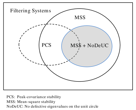
Figure 1: Relationships between the peak-covariance stability and mean-square stability over the space of the filtering systems under consideration. Theorem 3 indicates that the intersection of the two sets, PCS and MSS+NoDEUC, is contained in the set MSS.

Remark 4

In [22], for a scalar model with i.i.d. packet losses, it has been shown that the peak-covariance stability is equivalent to mean-square stability, while for a vector system even with i.i.d. packet losses, the relationship between the two is unclear. In [24], the equivalence between the two stability notions was established for systems that are one-step observable, again for the i.i.d. case. Theorem 3 now fills the gap for a large class of vector systems under general random packet drops.

4.2 The Critical $p-q$ Curve

In this subsection, we first show that for a fixed $q$ in the Gilbert-Elliott channel, there exists a critical failure rate $p_{c}$, such that if and only if the failure rate is below $p_{c}$, the Kalman filtering is mean-square stable. This conclusion is relatively independent of previous results, and the proof relies on a coupling argument and can be found in Appendix E.

Proposition 2

Let the recovery rate $q$ satisfy $|\lambda_{A}|^{2}(1-q)<1$. Then there exists a critical value $p_{c}\in(0,1]$ for the failure rate in the sense that

• $\sup_{k\in\mathbb{N}}\mathbb{E}\|P_{k}\|<\infty$ for all $\Sigma_{0}\geq 0$ and $0<p<p_{c}\leavevmode\nobreak\$;

• there exists $\Sigma_{0}\geq 0$ such that $\sup_{k\in\mathbb{N}}\mathbb{E}\|P_{k}\|=\infty$ for all $p_{c}<p<1$.

It has been shown in [25] that a necessary condition for mean-square stability of the filtering system is $|\lambda_{A}|^{2}(1-q)<1$, which is only related to the recovery rate $q$. For Gilbert-Elliot channels, a critical value phenomenon with respect to $q$ is also expectable. Theorem 4 proves the existence of the critical $p-q$ curve and Fig. 2 illustrates this critical curve in the $p-q$ plane. The proof, analogous to that of Proposition 2, is given in Appendix F.

Theorem 4

There exists a critical curve defined by $f_{c}(p,q)=0$, which reads two non-decreasing functions $p=p_{c}(q)$ and $q=q_{c}(p)$ with $q_{c}(\cdot)=p_{c}^{-1}(\cdot)$, dividing $(0,1)^{2}$ into two disjoint regions such that:

• If $(p,q)\in\big{\{}f_{c}(p,q)>0\big{\}}$, then $\sup_{k\in\mathbb{N}}\mathbb{E}\|P_{k}\|<\infty$ for all $\Sigma_{0}\geq 0$;

• If $(p,q)\in\big{\{}f_{c}(p,q)<0\big{\}}$, then there exists $\Sigma_{0}\geq 0$ under which $\sup_{k\in\mathbb{N}}\mathbb{E}\|P_{k}\|=\infty$.

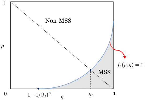
Figure 2: The $p-q$ plane is divided into MSS (Mean-Square Stability) and Non-MSS regions by the critical curve $f_{c}(p,q)=0$. When $p+q=1$, the Markovian packet loss process is reduced to an i.i.d. process. As a result, the intersection point of the curves $f_{c}(p,q)=0$ and $p+q=1$ gives the critical packet drop probability established in [36].

Remark 5

If the packet loss process is an i.i.d. process, where $p+q=1$ in the transition probability matrix defined in (3), Proposition 2 and Theorem 4 recover the result of Theorem 2 in [12]. It is worth pointing out that whether mean-square stability holds or not exactly on the curve $f_{c}(p,q)=0$ is beyond the reach of the current analysis (even for the i.i.d. case with $p+q=1$): such an understanding relies on the compactness of the stability or non-stability regions.

4.3 Mean-square Stability Conditions

We can now make use of the peak-covariance stability conditions we obtained in the last section, and the connection between peak-covariance stability and mean-square stability indicated in Theorem 3, to establish mean-square stability conditions for the considered Kalman filter. It turns out that the assumption requiring no defective eigenvalues on the unit circle, can be relaxed by an approximation method. We present the following result.

Theorem 5

Let the recovery rate $q$ satisfy $|\lambda_{A}|^{2}(1-q)<1$. Then there holds $p_{c}\geq\underline{p}$, where

$$\underline{p}\triangleq\sup\Big{\{}p:\exists(K,P)\mathrm{\leavevmode\nobreak\ s.t.\leavevmode\nobreak\ }\mathcal{L}_{K}(P)<P,P>0\Big{\}},$$ (14)

i.e., for all $\Sigma_{0}\geq 0$ and $0<p<\underline{p}$, the Kalman filtering system is mean-square stable.

The proof of Theorem 5 was given in Appendix G.

Remark 6

For second-order systems and certain classes of high-order systems, such as non-degenerate systems, necessary and sufficient conditions for mean-square stability have been derived in [25] and [27]. However, these results rely on a particular system structure and fail to apply to general LTI systems. It seems challenging to find an explicit description of necessary and sufficient conditions for mean-square stability of general LTI systems. Theorem 5 gives a stability criterion for general LTI systems.

5 Numerical Examples

In this section, we present two numerical examples to demonstrate the theoretical results we established in Sections 3 and 4.

5.1 Example I: A Second-order System

To compare with the works in [21, 22, 23], we will examine the same vector example considered therein. The parameters are specified as follows:

$$A=\left[\begin{array}[]{ccc}1.3&0.3\\ 0&1.2\end{array}\right],\leavevmode\nobreak\ \leavevmode\nobreak\ C=[1,1],$$

$Q=I_{2\times 2}$ and $R=1$. As illustrated in [22], it is easily checked that $\mathsf{I_{o}}=2$ and the spectrum of $A$ is $\sigma(A)=\{1.2,1.3\}$, and that $\lambda_{A}=1.3$.

First let us compare the sufficient condition we provide in Proposition 1 with the counterpart provided in [22]. Note that $|\lambda_{A}|^{2}(1-q)<1$ is a necessary condition for mean-square stability. We take $q=0.65$ as was done in [22]. As for the failure rate $p$, [22] concludes that $p<0.04$ guarantees peak-covariance stability; while Proposition 1 requires

$$p<\frac{1-|\lambda_{A}|^{2}(1-q)}{|\lambda_{A}|^{4}q},$$

which generates the less conservative condition $p<0.22$. In [22], all numerical simulations were implemented with parameters $(p,q)=(0.03,0.65)$. Note that, for the associated channel with $(p,q)=(0.04,0.65)$, $\mathbb{P}(\gamma_{k}=0)=0.0580$ when the packet loss process enters the stationary distribution, which means that the allowed long term packet loss rate is at most $5.80\%$. However, by choosing a larger $p$, Proposition 1 permits $\mathbb{P}(\gamma_{k}=0)=0.2529$ at the stationary distribution at most, i.e., the allowed long term packet dropout rate is $25.29\%$. Similarly, the example in [23] allows $p=0.1191$ at most. Separately, we note that it is rather convenient to check the condition in Proposition 1 even with manual calculation; in contrast, to check the conditions in [22] and [23] involves a considerable amount of numerical calculation.

In what follows, we use the criterion established in Theorem 2 to check for the peak-covariance stability. Then we obtain that when $p=1$ the LMI in 2) of Theorem 2 is still feasible. It should be pointed that at least for the parameters specified in this example, the criterion of [22] only covers the Gilbert-Elliott models with failure rate lower than $4.5\%$. Fig. 3 and Fig. 4 illustrate sample paths of $\|P_{k}\|$ and $\gamma_{k}$ with $(p,q)=(0.5,0.65)$ and $(p,q)=(0.99,0.65)$, respectively. The figures show that even a high value of $p$ may not effect the peak-covariance stability with the system parameters specified in this example, showing that Theorem 2 provides a less conservative criterion than Proposition 1 or [22, 23] does, a fact which is consistent with the theoretical analysis in Section 3.

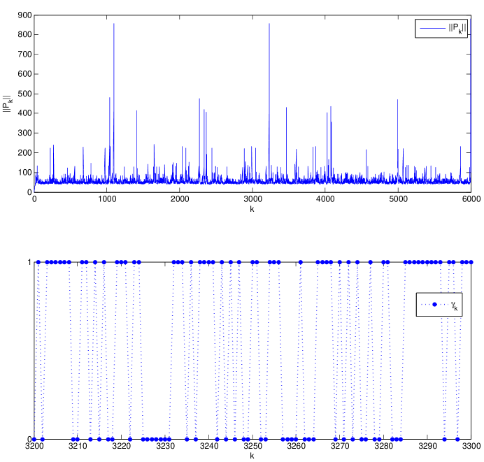
Figure 3: A sample path of $\|P_{k}\|$ and $\gamma_{k}$ with $p=0.5$, $q=0.65$ in Example I.

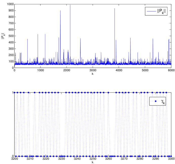
Figure 4: A sample path of $\|P_{k}\|$ and $\gamma_{k}$ with $p=0.99$, $q=0.65$ in Example I.

5.2 Example II: A Third-order System

To compare the work in Section 4 with the result [25] and [27], we will use the following example, where the parameters are given by

$$A=\left[\begin{array}[]{ccc}1.2&0&0\\ 0&1.2&0\\ 0&0&-1.2\end{array}\right],\leavevmode\nobreak\ \leavevmode\nobreak\ C=\left[\begin{array}[]{ccc}1&0&1\\ 0&1&1\end{array}\right],$$ (15)

$Q=I_{3\times 3}$ and $R=I_{2\times 2}$. In [25] and [27], mean-square stability of Kalman filtering for so-called non-degenerate systems has been studied. Before proceeding, we introduce their definition, which originates from [14].

Definition 5

Consider a system $(C,A)$ in diagonal standard form, i.e., $A=\mathrm{diag}(\lambda_{1},\ldots,\lambda_{n})$ and $C=[C_{1},\ldots,C_{n}]$. A quasi-equiblock of the system is defined as a subsystem $(C_{\mathcal{I}},A_{\mathcal{I}})$, where $\mathcal{I}\triangleq\{l_{1},\ldots,l_{i}\}\subset\{1.\ldots,n\}$, such that $A_{\mathcal{I}}=\mathrm{diag}(\lambda_{l_{1}},\ldots,\lambda_{l_{i}})$ with $|\lambda_{l_{1}}|=\cdots=|\lambda_{l_{i}}|$ and $C_{\mathcal{I}}=[C_{l_{1}},\ldots,C_{l_{i}}]$.

Definition 6

A diagonalizable system $(C,A)$ is non-degenerate if every quasi-equiblock of the system is one-step observable. Conversely, it is degenerate if it has at least one quasi-equiblock that is not one-step observable.

By the above definitions, the system in (15) is observable but degenerate since $|\lambda_{1}|=|\lambda_{2}|=|\lambda_{3}|$ but $(C,A)$ is not one-step observable. Hence none of the necessary and sufficient conditions developed in the aforementioned two papers is applicable in this example. To the best of our knowledge, no tool has been established so far to study mean-square stability of such a system. The results presented in Section 4 provide us a universal criterion for mean-square stability. Let us fix $q=0.5.$ We can conclude from Theorem 5 that if $p\leq 0.465$ the Kalman filter is mean-square stable. Fig. 5 illustrates a sample path of $\|P_{k}\|$ and $\gamma_{k}$ with $(p,q)=(0.45,0.5)$. Fig. 6 illustrates that with $(p,q)=(0.99,0.5)$ the expected prediction error covariance matrices diverge. One can verify that when $q=0.5$ and $p=1$ the criterion in Theorem 5 is violated as the LMI in Theorem 2 is infeasible.

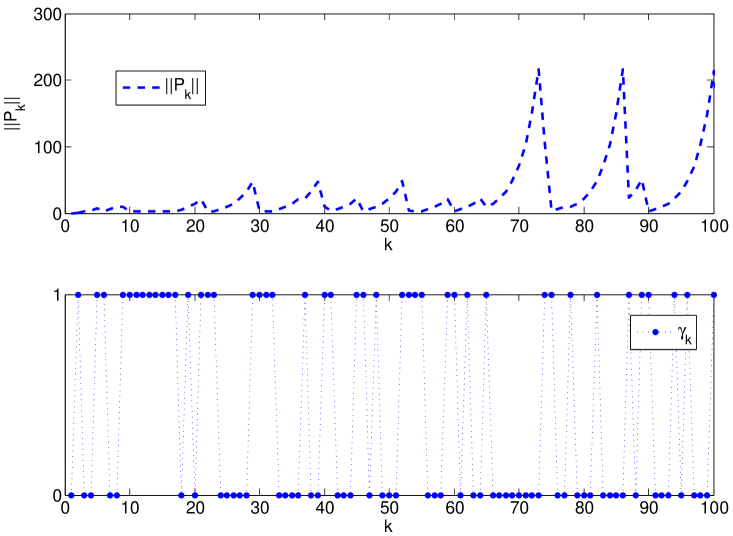
Figure 5: A sample path of $\|P_{k}\|$ and $\gamma_{k}$ with $p=0.45$, $q=0.5$ in Example II.

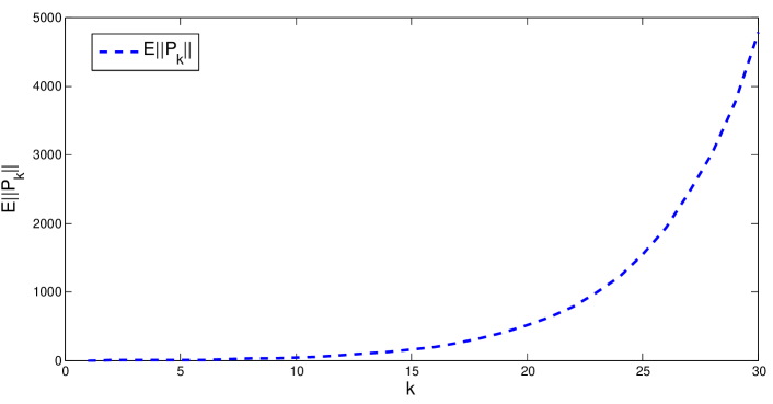
Figure 6: Divergence of $\mathbb{E}\|P_{k}\|$ with $p=0.99$, $q=0.5$ in Example II.

6 Conclusions

We have investigated the stability of Kalman filtering over Gilbert-Elliott channels. Random packet drop follows a time-homogeneous two-state Markov chain where the two states indicate successful or failed packet transmissions. We established a relaxed condition guaranteeing peak-covariance stability described by an inequality in terms of the spectral radius of the system matrix and transition probabilities of the Markov chain, and then showed that the condition can be reduced to an LMI feasibility problem. It was proved that peak-covariance stability implies mean-square stability if the system matrix has no defective eigenvalues on the unit circle. This connection holds for general random packet drop processes. We also proved that there exists a critical region in the $p-q$ plane such that if and only if the pair of recovery and failure rates falls into that region the expected prediction error covariance matrices are uniformly bounded. By fixing the recovery rate, a lower bound for the critical failure rate was obtained making use of the relationship between two stability criteria for general LTI systems. Numerical examples demonstrated significant improvement on the effectiveness of our appraoch compared with the existing literature.

Appendices. Proofs of Statements

Appendix A. Auxiliary Lemmas

In this section, we collect some lemmas that are regularly used throughout the proofs of our main results.

Lemma 3 (Lemma A.1 in [26])

For any matrices $X\geq Y\geq 0$, the following inequalities hold

$$h(X) \geq h(Y),$$ (16)

$$g(X) \geq g(Y),$$ (17)

$$h(X) \geq g(X),$$ (18)

where the operators $h$ and $g$ are defined in (4) and (5) respectively.

Lemma 4

Consider the operator

$$\phi_{i}({K}^{(i)},P) = (A^{i}+K^{(i)}C^{(i)})X(\cdot)^{*}+[A^{(i)}\leavevmode\nobreak\ K^{(i)}]\left[\begin{array}[]{ccc}Q^{(i)}&Q^{(i)}(D^{(i)})^{\prime}\\ \ast&D^{(i)}(Q^{(i)})(D^{(i)})^{\prime}+R^{(i)}\end{array}\right][A^{(i)}\leavevmode\nobreak\ K^{(i)}]^{*},$$

$$\leavevmode\nobreak\ \forall i\in\mathbb{N},$$

where $C^{(i)}=[C^{\prime},\leavevmode\nobreak\ A^{\prime}C^{\prime},\cdots,(A^{\prime})^{i-1}C^{\prime}]^{\prime}$, $A^{(i)}=[A^{i-1},\cdots,A,\leavevmode\nobreak\ I]$, $D^{(i)}=0$ for $i=1$ otherwise $D^{(i)}=\left[\begin{array}[]{cccc}0&0&\cdots&0\\ C&0&\cdots&0\\ \vdots&\vdots&\ddots&\vdots\\ CA^{i-2}&CA^{i-3}&\cdots&0\end{array}\right]$, $Q^{(i)}=\mathrm{diag}(\underbrace{Q,\cdots,Q}_{i})$, $R^{(i)}=\mathrm{diag}(\underbrace{R,\cdots,R}_{i})$, and $K^{(i)}$ are of compatible dimensions. For any $X\geq 0$ and $K^{(i)}$, it always holds that

$$g^{i}(X)=\min_{K^{(i)}}\phi_{i}(K^{(i)},X)\leq\phi_{i}(K^{(i)},X).$$

Proof. The result is readily established when setting $B=I$ in Lemmas 2 and 3 in [33]. For $i=1$, The result is well known as Lemma 1 in [12]. $\square$

Lemma 5 ([37])

For any $A\in\mathbb{C}^{n\times n}$, $\epsilon>0$ and $k\in\mathbb{N}$, it holds that

$$\|A^{k}\|\leq\sqrt{n}(1+2/\epsilon)^{n-1}\Big{(}|\lambda_{A}|+\epsilon\|A\|\Big{)}^{k}$$

Lemma 6 (Lemma 2 in [38])

For any $G\in\mathbb{C}^{n\times n}$ there exist $G_{i}\in\mathbb{S}^{n}_{+},\leavevmode\nobreak\ i=1,2,3,4$ such that

$$G=(G_{1}-G_{2})+(G_{3}-G_{4})\mathbf{i}$$

where $\mathbf{i}=\sqrt{-1}$.

Appendix B. Proof of Theorem 1

The proof relies on the following two lemmas.

Lemma 7 (Lemma 5 in [22])

Assume that $(C,A)$ is observable and $(A,Q^{{1}/{2}})$ is controllable. Define

$$\mathbb{S}_{0}^{n}=\{P:0\leq P\leq AP_{0}A^{\prime}+Q,\hbox{\leavevmode\nobreak\ for some\leavevmode\nobreak\ }P_{0}\geq 0\},$$

Then there exists a constant $\mathsf{L}>0$ such that

1. for any $X\in\mathbb{S}_{0}^{n}$, $g^{k}(X)\leq\mathsf{L}I$ for all $k\geq\mathsf{I_{o}}$;

2. for any $X\in\mathbb{S}_{+}^{n}$, $g^{k+1}(X)\leq\mathsf{L}I$ for all $k\geq\mathsf{I_{o}}$,

where the operator $g$ is defined in (5).

Lemma 8

For $q\in(0,1)$ and $A\in\mathbb{R}^{n\times n}$, the series of matrices $\sum_{i=1}^{\infty}(A\otimes A)^{i}(1-q)^{i-1}q$ and $\sum_{i=1}^{\infty}\sum_{j=0}^{i-1}(A\otimes A)^{j}(1-q)^{i-1}q$ converge if and only if $|\lambda_{A}|^{2}(1-q)<1$.

Proof. First observe that

$$\sum_{i=1}^{\infty}\sum_{j=0}^{i-1}(A\otimes A)^{j}(1-q)^{i-1}q=\sum_{i=0}^{\infty}(A\otimes A)^{i}(1-q)^{i}.$$

The geometric series generated by $(A\otimes A)(1-q)$ converges if and only if $|\lambda_{A\otimes A}|(1-q)<1$. Therefore the conclusion follows from the fact that $|\lambda_{A\otimes A}|=\max\{|\lambda_{i}\lambda_{j}|:\lambda_{i},\lambda_{j}\in\sigma(A)\}=|\lambda_{A}|^{2}$. $\square$

Now fix $j\geq 1$. First note that, for any $k\in[\tau_{j+1},\beta_{j+1}-1]$, $\gamma_{k}=0$. Hence we have

$$P_{\beta_{j+1}} = \sum_{i=1}^{\infty}1_{\{\beta_{j+1}^{*}=i\}}h^{i}(P_{\tau_{j+1}})$$ (20)

$$\triangleq \sum_{i=1}^{\infty}1_{\{\beta_{j+1}^{*}=i\}}A^{i}P_{\tau_{j+1}}(A^{i})^{\prime}+\sum_{i=1}^{\infty}1_{\{\beta_{j+1}^{*}=i\}}V_{i},$$

where $V_{i}\triangleq\sum_{l=0}^{i-1}A^{l}Q(A^{l})^{\prime}$. Now let us consider the interval $[\beta_{j},\tau_{j+1}-1]$ over which $\tau_{j+1}^{*}$ packets are successfully received. We will analyze the relationship between $P_{\tau_{j+1}}$ and $P_{\beta_{j}}$ in two separated cases, which are $\tau_{j+1}^{*}\leq\mathsf{I_{o}}-1$ and $\tau_{j+1}^{*}\geq\mathsf{I_{o}}$. Computation yields the following result

$$P_{\tau_{j+1}} = \sum_{i=1}^{\mathsf{I_{o}}-1}1_{\{\tau_{j+1}^{*}=i\}}g^{i}(P_{\beta_{j}})+\sum_{l=\mathsf{I_{o}}}^{\infty}1_{\{\tau_{j+1}^{*}=l\}}g^{l}(P_{\beta_{j}})$$ (21)

$$\leq \sum_{i=1}^{\mathsf{I_{o}}-1}1_{\{\tau_{j+1}^{*}=i\}}g^{i}(P_{\beta_{j}})+\mathsf{L}I\sum_{l=\mathsf{I_{o}}}^{\infty}1_{\{\tau_{j+1}^{*}=l\}}$$

$$\leq \sum_{i=1}^{\mathsf{I_{o}}-1}1_{\{\tau_{j+1}^{*}=i\}}\phi_{i}(K^{(i)},P_{\beta_{j}})+\mathsf{L}I\sum_{l=\mathsf{I_{o}}}^{\infty}1_{\{\tau_{j+1}^{*}=l\}}$$

$$= \sum_{i=1}^{\mathsf{I_{o}}-1}1_{\{\tau_{j+1}^{*}=i\}}(A^{i}+K^{(i)}C^{(i)})P_{\beta_{j}}(A^{i}+K^{(i)}C^{(i)})^{*}+\mathsf{L}I\sum_{j=\mathsf{I_{o}}}^{\infty}1_{\{\tau_{j+1}^{*}=l\}}$$

$$\hskip 85.35826pt+\sum_{i=1}^{\mathsf{I_{o}}-1}1_{\{\tau_{j+1}^{*}=i\}}[A^{i}\leavevmode\nobreak\ K^{(i)}]J_{i}[A^{i}\leavevmode\nobreak\ K^{(i)}]^{*}$$

$$\triangleq (A^{i}+K^{(i)}C^{(i)})P_{\beta_{j}}(A^{i}+K^{(i)}C^{(i)})^{*}+U,$$

where $J_{i}\triangleq\left[\begin{array}[]{ccc}Q^{(i)}&Q^{(i)}(D^{(i)})^{\prime}\\ D^{(i)}(Q^{(i)})&D^{(i)}(Q^{(i)})(D^{(i)})^{\prime}+R^{(i)}\end{array}\right]$ and

$$U\triangleq\mathsf{L}I\sum_{j=\mathsf{I_{o}}}^{\infty}1_{\{\tau_{j+1}^{*}=l\}}+\sum_{i=1}^{\mathsf{I_{o}}-1}1_{\{\tau_{j+1}^{*}=i\}}[A^{i}\leavevmode\nobreak\ K^{(i)}]J_{i}[A^{i}\leavevmode\nobreak\ K^{(i)}]^{*}$$

is bounded. The first inequality is from Lemma 7 and the second one follows from Lemma 4. By substituting (21) into (20), it yields

$$P_{\beta_{j+1}} \leq \sum_{i=1}^{\infty}1_{\{\beta_{j+1}^{*}=i\}}A^{i}\left[\sum_{l=1}^{\mathsf{I_{o}}-1}1_{\{\tau_{j+1}^{*}=l\}}(A^{l}+K^{(l)}C^{(l)})P_{\beta_{j}}(A^{l}+K^{(l)}C^{(l)})^{*}\right](A^{i})^{\prime}+W,$$ (22)

where $W\triangleq\sum_{i=1}^{\infty}1_{\{\beta_{j+1}^{*}=i\}}A^{i}U(A^{i})^{\prime}+\sum_{i=1}^{\infty}1_{\{\beta_{j+1}^{*}=i\}}V_{i}$.

To facilitate discussion, we force $P_{\beta_{j+1}}$ in (22) to take the maximum,

$$P_{\beta_{j+1}}=\sum_{i=1}^{\infty}1_{\{\beta_{j+1}^{*}=i\}}A^{i}\left[\sum_{l=1}^{\mathsf{I_{o}}-1}1_{\{\tau_{j+1}^{*}=l\}}(A^{l}+K^{(l)}C^{(l)})P_{\beta_{j}}(A^{l}+K^{(l)}C^{(l)})^{*}\right](A^{i})^{\prime}+W.$$ (23)

In what follow, we only take (23) into consideration. For other cases in (22), the subsequent conclusion still holds as (23) renders an upper envelop of $\{P_{\beta_{j}}\}_{j\in\mathbb{N}}$.

We introduce the vectorization operator. Let $X=[x_{1}\leavevmode\nobreak\ x_{2}\leavevmode\nobreak\ \cdots\leavevmode\nobreak\ x_{n}]\in\mathbb{C}^{m\times n}$ where $x_{i}\in\mathbb{C}^{m}$. Then we define

$$\mathrm{vec}(X)\triangleq\left[x_{1}^{\prime},x_{2}^{\prime},\ldots,x_{n}^{\prime}\right]^{\prime}\in\mathbb{C}^{mn}.$$

Notice that $\mathrm{vec}(AXB)=(B^{\prime}\otimes A)\mathrm{vec}(X)$. For Kronecker product, we have $\left(A_{1}A_{2}\right)\otimes\left(B_{1}B_{2}\right)=\left(A_{1}\otimes B_{1}\right)\left(A_{2}\otimes B_{2}\right)$. Take expectations and vectorization operators over both sides of (22). We obtain from Lemma 1 that

$$\mathbb{E}[\mathrm{vec}(P_{\beta_{j+1}})] = \mathbb{E}[\mathrm{vec}(W)]$$

$$+\sum_{i=1}^{\infty}(A\otimes A)^{i}(1-q)^{i-1}q\sum_{l=1}^{\mathsf{I_{o}}-1}\overline{(A^{l}+K^{(l)}C^{(l)})}\otimes(A^{l}+K^{(l)}C^{(l)})p(1-p)^{l-1}\,\mathbb{E}[\mathrm{vec}(P_{\beta_{j}})].$$

In the above equation $\mathbb{E}[\mathrm{vec}(W)]$ can be written as

$$\mathbb{E}[\mathrm{vec}(W)] = \sum_{i=1}^{\infty}(A\otimes A)^{i}(1-q)^{i-1}q\,\mathrm{vec}(U)+\sum_{i=1}^{\infty}\sum_{l=0}^{i-1}(A\otimes A)^{l}(1-q)^{i-1}q\,\mathrm{vec}(Q).$$ (25)

In Lemma 8, we show that both of the two terms in (25) converges if $|\lambda_{A}|^{2}(1-q)<1$.

For $j=1$, following the similar argument as above, we have

$$\mathbb{E}\|P_{\beta_{1}}\|\leq\mathbb{E}\|P_{\tau_{1}}\|\sum_{i=1}^{\infty}\|A^{i}\|^{2}(1-q)^{i-1}q+\Big{\|}\sum_{i=1}^{\infty}(1-q)^{i-1}qV_{i}\Big{\|},$$

where $V_{i}$’s are defined in (20). Moreover, by Lemma 7 and (18), it holds that

$$\mathbb{E}\|P_{\tau_{1}}\| \leq \|\mathsf{L}I\|+\sum_{i=1}^{\mathsf{I_{o}}}\|g^{i}(\Sigma_{0})\|(1-p)^{i-1}p$$

$$\leq \|\mathsf{L}I\|+\|\Sigma_{0}\|\sum_{i=1}^{\mathsf{I_{o}}}\|A^{i}\|^{2}(1-p)^{i-1}p+\|V_{\mathsf{I_{o}}}\|,$$

showing that $\mathbb{E}\|P_{\tau_{1}}\|$ is bounded. To sum up, $\mathbb{E}\|P_{\beta_{1}}\|$ is bounded if $|\lambda_{A}|^{2}(1-q)<1$. By applying the Cauchy-Schwarz inequality to the inner product of random variables, the boundness of $\mathbb{E}\|P_{\beta_{1}}\|$ implies the boundness of each element of $\mathbb{E}[P_{\beta_{1}}]$. So is $\mathbb{E}[\mathrm{vec}(P_{\beta_{1}})]$ if $|\lambda_{A}|^{2}(1-q)<1$.

We have shown that $\mathbb{E}[\mathrm{vec}(P_{\beta_{j}})]$ for $j\in\mathbb{N}$ evolves following (Appendix B. Proof of Theorem 1), and that $\mathbb{E}[\mathrm{vec}(W)]$ in (Appendix B. Proof of Theorem 1) and $\mathbb{E}[\mathrm{vec}(P_{\beta_{1}})]$ are bounded if $|\lambda_{A}|^{2}(1-q)<1$. We conclude that if $|\lambda_{A}|^{2}(1-q)<1$ and there exists an $K\triangleq[K^{(1)},\ldots,K^{(\mathsf{I_{o}}-1)}]$ such that $|\lambda_{H(K)}|$ defined in (7) is less than $1$, then the spectral radius of

$$\sum_{i=1}^{\infty}(A\otimes A)^{i}(1-q)^{i-1}q\sum_{l=1}^{\mathsf{I_{o}}-1}\overline{(A^{l}+K^{(l)}C^{(l)})}\otimes(A^{l}+K^{(l)}C^{(l)})(1-p)^{l-1}p$$

is less than $1$, all the above observations lead to $\sup_{j\geq 1}\mathbb{E}[\mathrm{vec}_{i}(P_{\beta_{j}})]<\infty\leavevmode\nobreak\ \forall 1\leq i\leq n^{2}$, where $\mathrm{vec}_{i}(X)$ represents the $i$th element of $\mathrm{vec}(X)$. In addition, there holds

$$\mathbb{E}\|P_{\beta_{j}}\|\leq\mathbb{E}\left[\mathrm{tr}(P_{\beta_{j}})\right]=[e_{1}^{\prime},\ldots,e_{n}^{\prime}]\,\mathbb{E}[\mathrm{vec}(P_{\beta_{j}})],$$

where $e_{i}$ denotes the vector with a $1$ in the $i$th coordinate and 0’s elsewhere, so the desired result follows.

Appendix C. Proof of Theorem 2

$(i)\Rightarrow(ii)$. It suffices to show $|\lambda_{H^{*}(K)}|<1$. The hypothesis means that for any $X\in\mathbb{S}_{+}^{n}$

$$\lim_{k\rightarrow\infty}\left(H^{*}(K)\right)^{k}\mathrm{vec}(X)=0.$$ (26)

In light of Lemma 6, for any $G\in\mathbb{C}^{n\times n}$ there exist $G_{1},G_{2},G_{3},G_{4}\in\mathbb{S}_{+}^{n}$ such that $G=(G_{1}-G_{2})+(G_{3}-G_{4})\mathbf{i}$. It can been seen from (26) that

$$\lim_{k\rightarrow\infty}\left(H^{*}(K)\right)^{k}\mathrm{vec}(G)$$

$$= \lim_{k\rightarrow\infty}\left(H^{*}(K)\right)^{k}\Big{(}\mathrm{vec}(G_{1})-\mathrm{vec}(G_{2})+\mathrm{vec}(G_{3})\mathbf{i}-\mathrm{vec}(G_{4})\mathbf{i}\Big{)}$$

$$= 0,$$

which implies $(ii)$.

$(ii)\Rightarrow(iii)$. Since $|\lambda_{H^{*}(K)}|<1$ by the hypothesis in $(ii)$, $(I-H^{*}(K))^{-1}$ exist and it equals to $\sum_{i=0}^{\infty}\left(H^{*}(K)\right)^{i}$. Due to the nonsingular of $(I-H^{*}(K))^{-1}$ and the one-to-one correspondence of vectorization operator, for any positive definite matrix $V\in\mathbb{C}^{n\times n}$, there exists a unique matrix $P\in\mathbb{C}^{n\times n}$ such that

$$\mathrm{vec}(V)=\left(I-H^{*}(K)\right)\mathrm{vec}(P).$$ (27)

The property of Kronecker product gives $\mathrm{vec}(V)=\mathrm{vec}\left(P-\mathcal{L}_{K}(P)\right).$ Since vectorization is one-to-one correspondence, we then have $V=P-\mathcal{L}_{K}(P)>0.$ It still remains to show $P>0$. It follows from (28) that

$$\mathrm{vec}(P) = \left(I-H^{*}(K)\right)^{-1}\mathrm{vec}(V)$$ (28)

$$= \sum_{i=0}^{\infty}\left(H^{*}(K)\right)^{i}\mathrm{vec}(V)$$

$$= \mathrm{vec}\left(\sum_{i=0}^{\infty}\mathcal{L}_{K}^{i}(V)\right),$$

which yields $P=\sum_{i=0}^{\infty}\mathcal{L}_{K}^{i}(V)>0.$

$(iii)\Rightarrow(i)$. If there exist $\,K=[K^{(1)},\ldots,K^{(\mathsf{I_{o}}-1)}]$ with each matrix $K^{(i)}$ having compatible dimensions and $P>0$ such that $\mathcal{L}_{K}(P)<P$, then there must exist a $\mu\in(0,1)$ satisfying $\mathcal{L}_{K}(P)<\mu P$. Choose an $c>0$ such that $X\leq cP$. Then, due to the linearity and non-decreasing properties of $\mathcal{L}_{K}(X)$ with respect to $X$ on the positive semi-definite cone, for $k\in\mathbb{N}$

$$\mathcal{L}^{k}_{K}(X)\leq\mathcal{L}^{k}_{K}(cP)=c\mathcal{L}^{k}_{K}(P)<c\mathcal{L}^{k-1}_{K}(\mu P)<\cdots<c\mu^{k}P,$$

which leads to $\lim_{k\rightarrow\infty}\mathcal{L}^{k}_{K}(X)=0$.

$(iii)\Rightarrow(iv)$. It can be seen from $(iii)$ that

$$p\sum_{i=1}^{\mathsf{I_{o}}-1}(1-p)^{i-1}(A^{i}+K^{(i)}C^{(i)})^{*}Y(A^{i}+K^{(i)}C^{(i)})<P,\leavevmode\nobreak\ \leavevmode\nobreak\ P>0$$ (29)

and $Y$ is the solution to the following Lyapunov equation

$$Y=(1-q)A^{\prime}YA+qA^{\prime}PA,$$ (30)

where $qA^{\prime}PA>0$ due to $q>0$, $P>0$ and non-singularity of $A$. In light of the Schur Complement lemma, (29) is equivalent to

$$\Xi\triangleq\left[\begin{array}[]{ccccccc}P&\sqrt{p}(A+KC)^{*}&\cdots&\sqrt{p(1-p)^{\mathsf{I_{o}}-2}}(A^{\mathsf{I_{o}}-1}+K^{(i)}C^{(i)})^{*}\\ &Y^{-1}&\cdots&0\\ \vdots&\vdots&\ddots&\vdots\\ &*&\cdots&Y^{-1}\end{array}\right]>0.$$

Then we obtain

$$\left[\begin{array}[]{cccc}I&0&\cdots&0\\ 0&Y&\cdots&0\\ \vdots&\vdots&\ddots&\vdots\\ 0&0&\cdots&Y\end{array}\right]\Xi\left[\begin{array}[]{cccc}I&0&\cdots&0\\ 0&Y&\cdots&0\\ \vdots&\vdots&\ddots&\vdots\\ 0&0&\cdots&Y\end{array}\right]=\Psi.$$

The equality holds by letting $F_{i}=(YK^{(i)})^{*},\leavevmode\nobreak\ i=1,\dots,\mathsf{I_{o}}-1$, thereby (13) follows. By relaxing the equality in (30) into inequality and applying the same method as above, (12) follows.

$(iv)\Rightarrow(iii)$. Note that, by the Schur complement lemma and $X,Y>0$, (12) holds if and only if

$$Y\geq(1-q)A^{\prime}YA+qA^{\prime}XA.$$ (32)

Similarly, (13) holds if and only if

$$p\sum_{i=1}^{\mathsf{I_{o}}-1}(1-p)^{i-1}(A^{i}+K^{(i)}C^{(i)})^{*}Y(A^{i}+K^{(i)}C^{(i)})<X,$$ (33)

where $K^{(i)}=Y^{-1}F_{i}^{*},\leavevmode\nobreak\ i=1,\ldots,\mathsf{I_{o}}-1$. Applying the inequality of (32) for $k$ times, it results in

$$Y\geq(1-q)^{k}(A^{\prime})^{k}YA^{k}+q\sum_{j=1}^{k}(1-q)^{j-1}(A^{\prime})^{j}XA^{j}.$$

As $Y$ is bounded, taking limitation on the right sides, it yields

$$Y\geq q\sum_{j=1}^{\infty}(1-q)^{j-1}(A^{\prime})^{j}XA^{j}.$$ (34)

Combining (33) and (34), we obtain $\mathcal{L}_{K}(X)<X$, where $(iii)$ follows.

Appendix D. Proof of Theorem 3

To prove this theorem, we need some preliminary lemmas.

Lemma 9

Suppose that there exist constants $d_{1},d_{0}\geq 0$ such that, for any $j\in\mathbb{N}$ and $k\in[\beta_{j},\beta_{j+1}]$, $\|P_{k}\|\leq\max\limits_{i=j,j+1}\{d_{1}\|P_{\beta_{i}}\|+d_{0}\}$ holds $\mu-$almost surely. If $\sup_{j\in\mathbb{N}}\mathbb{E}\|P_{\beta_{j}}\|<\infty$, then $\sup_{k\in\mathbb{N}}\mathbb{E}\|P_{k}\|<\infty$ holds.

Proof. Since $\sup_{j\in\mathbb{N}}\mathbb{E}\|P_{\beta_{j}}\|<\infty$, there exists a uniform bound $\alpha$ for $\{\mathbb{E}\|P_{\beta_{j}}\|\}_{j\in\mathbb{N}}$, i.e., $\mathbb{E}\|P_{\beta_{j}}\|\leq\alpha$ for all $j\in\mathbb{N}$. By the definition of $\beta_{j}$ in (6), $k$ should be no larger than $\beta_{k}$ for all $k\in\mathbb{N}$. Then one obtains

$$\mathbb{E}\|P_{k}\| = \mathbb{E}\left[\sum_{j=0}^{k-1}\mathbb{E}\Big{[}\|P_{k}\|\mid\beta_{j}\leq k\leq\beta_{j+1}\Big{]}1_{\{\beta_{j}\leq k\leq\beta_{j+1}\}}\right]$$

$$\leq \sum_{j=0}^{k-1}\mathbb{E}\left[\max_{i=j,j+1}\{d_{1}\|P_{\beta_{i}}\|+d_{0}\}\mid\beta_{j}\leq k\leq\beta_{j+1}\right]\mu(\beta_{j}\leq k\leq\beta_{j+1})$$

$$\leq \sum_{j=0}^{k-1}\left(d_{1}\mathbb{E}\|P_{\beta_{j}}\|+d_{1}\mathbb{E}\|P_{\beta_{j+1}}\|+d_{0}\right)\mu(\beta_{j}\leq k\leq\beta_{j+1})$$

$$\leq \left(2d_{1}\sup_{j\leq k}\mathbb{E}\|P_{\beta_{j}}\|+d_{0}\right)\sum_{j=0}^{k-1}\mu(\beta_{j}\leq k\leq\beta_{j+1})$$

$$\leq 2d_{1}\alpha+d_{0},$$

which completes the proof. $\square$

Before proceeding to the proof of the theorem, let us provide some properties related to the discrete-time algebraic Riccati equation (DARE). The proof, provided in [39], is omitted.

Lemma 10

Consider the following DARE

$$P=APA^{\prime}+Q-APC^{\prime}(CPC^{\prime}+R)^{-1}CPA^{\prime}.$$ (35)

If $(A,{Q}^{{1}/{2}})$ is controllable and $(C,A)$ is observable, then it has a unique positive definite solution $\tilde{P}$ and $A+\tilde{K}C$ is stable, where $\tilde{K}=-A\tilde{P}C^{\prime}(C\tilde{P}C^{\prime}+R)^{-1}$.

Fix $j\geq 0$. First of all, we shall show that, for $k\in[\beta_{j}+1,\tau_{j+1}]$, $\|P_{k}\|$ is uniformly bounded by an affine function of $\|P_{\beta_{j}}\|$. By Lemma 4 and Lemma 10, we have $g(P_{k-1})\leq\phi_{1}(\tilde{K},P_{k-1})$ and that $A+\tilde{K}C$ is stable. In light of (17) in Lemma 3, we further obtain $g^{i}(P_{k-1})\leq\phi_{1}^{i}(\tilde{K},P_{k-1})$ for all $i\in\mathbb{N}$. Therefore, an upper bound of $\|P_{k}\|$ is given as follows:

$$\|P_{k}\| = \|g^{k-\beta_{j}}(P_{\beta_{j}})\|$$

$$\leq \|\phi_{1}^{k-\beta_{j}}(\tilde{K},P_{\beta_{j}})\|$$

$$\leq \Big{\|}(A+\tilde{K}C)^{k-\beta_{j}}P_{\beta_{j}}(A^{\prime}+C^{\prime}\tilde{K}^{*})^{k-\beta_{j}}\Big{\|}+\Big{\|}\sum_{i=0}^{k-\beta_{j}-1}(A+\tilde{K}C)^{i}(Q+\tilde{K}R\tilde{K}^{*})(A^{\prime}+C^{\prime}\tilde{K}^{*})^{i}\Big{\|}$$

$$\leq \|(A+\tilde{K}C)^{k-\beta_{j}}\|^{2}\|P_{\beta_{j}}\|+\sum_{i=0}^{k-\beta_{j}-1}\|(A+\tilde{K}C)^{i}\|^{2}\|Q+\tilde{K}R\tilde{K}^{*}\|$$

$$\leq m_{0}\,\alpha_{0}^{2k-2\beta_{j}}\|P_{\beta_{j}}\|+m_{0}\|Q+\tilde{K}R\tilde{K}^{*}\|\sum_{i=0}^{k-\beta_{j}-1}\alpha_{0}^{2i},$$

where $\alpha_{0}=|\lambda_{A+\tilde{K}C}|+\epsilon_{0}\|A+\tilde{K}C\|$ and $m_{0}=n(1+2/\epsilon_{0})^{2n-2}$ with a positive number $\epsilon_{0}$ satisfying $|\lambda_{A+\tilde{K}C}|+\epsilon_{0}\|A+\tilde{K}C\|<1$ (such an $\epsilon_{0}$ must exist because $|\lambda_{A+\tilde{K}C}|<1$), and the last inequality holds due to Lemma 5. Observe that $\sum_{i=0}^{k-\beta_{j}-1}\alpha_{0}^{2i}\leq\frac{1}{1-\alpha_{0}^{2}}$. As $\alpha_{0}<1$, $\alpha_{0}^{2k-2\beta_{j}}<1$ for any $k\in[\beta_{j}+1,\tau_{j+1}]$. Therefore,

$$\|P_{k}\|\leq m_{0}\|P_{\beta_{j}}\|+n_{0},$$ (36)

where $n_{0}\triangleq\frac{m_{0}}{1-\alpha_{0}^{2}}\|Q+\tilde{K}R\tilde{K}^{\prime}\|$.

Next, we shall show that, for $k\in[\tau_{j+1}+1,\beta_{j+1}]$, $\|P_{k}\|$ is bounded by an affine function of $\|P_{\beta_{j+1}}\|$. To do this, let us look at the relationship between $P_{\beta_{j+1}}$ and $P_{k}$. Since $\gamma_{k}=0$ for all $k\in[\tau_{j+1},\beta_{j+1}-1]$, the relation is given by

$$P_{\beta_{j+1}}=A^{\beta_{j+1}-j}P_{k}(A^{\prime})^{\beta_{j+1}-k}+\sum_{i=0}^{\beta_{j+1}-k-1}A^{i}Q(A^{\prime})^{i},$$

from which we obtain $P_{\beta_{j+1}}\geq A^{\beta_{j+1}-k}P_{k}(A^{\prime})^{\beta_{j+1}-k}.$ Then it yields

$$\|P_{\beta_{j+1}}\| \geq \|A^{\beta_{j+1}-k}P_{k}(A^{\prime})^{\beta_{j+1}-k}\|$$

$$\geq \frac{1}{n}\mathrm{Tr}(A^{\beta_{j+1}-k}P_{k}(A^{\prime})^{\beta_{j+1}-k})$$

$$= \frac{1}{n}\mathrm{Tr}(P_{k}^{{1}/{2}}(A^{\prime})^{\beta_{j+1}-k}A^{\beta_{j+1}-k}P_{k}^{{1}/{2}})$$

$$\geq \frac{1}{n}\|A^{k-\beta_{j+1}}\|^{-2}\mathrm{Tr}(P_{j})$$

$$\geq \frac{1}{n}\|A^{k-\beta_{j+1}}\|^{-2}\|P_{k}\|,$$

where the second and the last inequality allows from the fact that $\|X\|=\lambda_{X}\geq\frac{1}{n}\mathrm{Tr}(X)$ and $\mathrm{Tr}(X)\geq\|{X}\|$ for any $X\in\mathbb{S}_{+}^{n}$; the third one holds since

$$(A^{\prime})^{\beta_{j+1}-k}A^{\beta_{j+1}-k}\geq\min\sigma\big{(}A^{\beta_{j+1}-k}(\cdot)^{\prime}\big{)}I=\frac{1}{\lambda_{A^{k-\beta_{j+1}}(\cdot)^{\prime}}}I=\|A^{k-\beta_{j+1}}\|^{-2}I.$$

If $A$ has no eigenvalues on the unit circle, by Lemma 5, there holds $\|A^{k-\beta_{j+1}}\|\leq n_{1}\,\alpha_{1}^{\beta_{j+1}-k}$ where $n_{1}\triangleq\sqrt{n}(1+2/\epsilon_{1})^{n-1}$ and $\alpha_{1}\triangleq|\lambda_{A^{-1}}|+\epsilon_{1}\|A^{-1}\|$ with a positive number $\epsilon_{1}$ so that $\alpha_{1}<1$ (such an $\epsilon_{1}$ must exist since $|\lambda_{A^{-1}}|<1$ by assumption (A1)). As $\alpha_{1}<1$, $\|A^{k-\beta_{j+1}}\|\leq n_{1}\,\alpha_{1}^{\beta_{j+1}-k}<n_{1}$ for all $k\in[\beta_{j}+1,\tau_{j+1}]$. If $A$ has semi-simple eigenvalues on the unit circles, we denote the Jordan form of $A$ as $J=\mathrm{diag}(J_{11},J_{22})$, where $A_{11}$ has no eigenvalues on the unit circle and $A_{22}$ is diagonal with all semi-simple eigenvalues on the unit circle, i.e., there exists a nonsingular matrix $S\in\mathbb{R}^{n\times n}$ such that $J=SAS^{-1}.$ In this case,

$$\|J^{k-\beta_{j+1}}\|=\max\left\{\|J_{11}^{k-\beta_{j+1}}\|,\|J_{22}^{k-\beta_{j+1}}\|\right\}\leq\max\{n_{1},1\}\leq n_{1},$$

where, similarly, $n_{1}\triangleq\sqrt{n}(1+2/\epsilon_{1})^{n-1}$ with a positive number $\epsilon_{1}$ so that $|\lambda_{J_{11}^{-1}}|+\epsilon_{1}\|J_{11}^{-1}\|<1$. Since $\|S^{-1}\cdot S\|$ can be considered a matrix norm, we have

$$\|A^{k-\beta_{j+1}}\|=\|S^{-1}J^{k-\beta_{j+1}}S\|\leq c\|J^{k-\beta_{j+1}}\|\leq cn_{1},$$

where $c=\sup_{X\in\mathbb{C}^{n\times n}}\frac{\|S^{-1}XS\|}{\|X\|}<\infty$ due to the equivalence of matrix norms on a finite dimensional vector space. Then, we have the following upper bound for $\|P_{k}\|$ for all $k\in[\tau_{j+1}+1,\beta_{j+1}]$:

$$\|P_{k}\|\leq n\|A^{k-\beta_{j+1}}\|^{2}\|P_{\beta_{j+1}}\|\leq m_{1}\|P_{\beta_{j+1}}\|,$$ (37)

where $m_{1}\triangleq nc^{2}n_{1}^{2}$.

According to (36) and (37), it can be seen that when $k\in[\beta_{j},\beta_{j+1}]$

$$\|P_{k}\|\leq\max\{m_{0},m_{1}\}\max\{\|P_{\beta_{j}}\|,\|P_{\beta_{j+1}}\|\}+n_{0}.$$

Since $j$ is arbitrarily chosen, by invoking Lemma 9, the desired conclusion follows.

Appendix E. Proof of Proposition 2

If $p=0$, we have the standard Kalman filter, which evidently converges to a bounded estimation error covariance. On the other hand, if $p=1$, then the Kalman filter reduces to an open-loop predictor after time step $k=2$, which suggests that there exists a transition point for $p$ beyond which the expected prediction error covariance matrices are not uniformly bounded. It remains to show that with a given $q$ this transition point is unique. Fix a $0\leq p_{1}<1$ such that $\sup_{k\in\mathbb{N}}\mathbb{E}_{p_{1}}\|P_{k}\|<\infty\leavevmode\nobreak\ \forall\Sigma_{0}\geq 0$. It suffices to show that, for any $p_{2}<p_{1}$, $\sup_{k\in\mathbb{N}}\mathbb{E}_{p_{2}}\|P_{k}\|<\infty$ for all $\Sigma_{0}\geq 0$. To differentiate two Markov chains with different failure rate in (3), we use the notation $\{\gamma_{k}(p_{i})\}_{k\in\mathbb{N}}$ instead to represent the packet loss process so as to indicate the configuration $p=p_{i}$ in (3). We will prove the aforementioned statement using a coupling argument. We define a sequence of random vectors $\{(z_{k},\tilde{z}_{k})\}_{k\in\mathbb{N}}$ over a probability space $(\mathscr{G},\mathcal{G},\pi)$ with $\mathscr{G}=\{(0,0),(0,1),(1,1)\}^{\mathbb{N}}$ and $\mathcal{G}_{k}$ representing the filtration generated by $(z_{1},\tilde{z}_{1}),\ldots,(z_{k},\tilde{z}_{k})$. We also define

$$\varphi_{1}(\{z_{k},\tilde{z}_{k}\}_{k=1:t})=\psi_{z_{t}}\circ\cdots\circ\psi_{z_{1}}(\Sigma_{0})$$

and

$$\varphi_{2}(\{z_{k},\tilde{z}_{k}\}_{k=1:t})=\psi_{\tilde{z}_{t}}\circ\cdots\circ\psi_{\tilde{z}_{1}}(\Sigma_{0}),$$

where $\psi_{z}=zg+(1-z)h$ with $h,g$ defined in (4), (5) and $z=\{0,1\}$. Due to Lemma 3 and $z_{k}\leq\tilde{z}_{k}$ in $\mathscr{G}$, we have $\varphi_{1}\left(\{z_{k},\tilde{z}_{k}\}_{k=1:t}\right)\geq\varphi_{2}\left(\{z_{k},\tilde{z}_{k}\}_{k=1:t}\right)$.

When $p_{2}+q\leq 1$, we let the evolution of $\{(z_{k},\tilde{z}_{k})\}_{k\in\mathbb{N}}$ follow the Markov chain illustrated in Fig. 7, whereby it can seen that $\pi(z_{k+1}=j|z_{k}=i)$’s for $i,j=\{0,1\}$ are constants independent of $\tilde{z}_{k}$’s, and conversely that $\pi(\tilde{z}_{k}=j|\tilde{z}_{k}=i)$’s for $i,j=\{0,1\}$ are constants independent of $z_{k}$’s. Therefore, both the marginal distributions of $\{z_{k}\}_{k\in\mathbb{N}}$ and $\{\tilde{z}_{k}\}_{k\in\mathbb{N}}$ are Markovian, and moreover,

$$\pi(z_{k+1}=j|z_{k}=i)=\mathbb{P}_{p_{1}}(\gamma_{k+1}(p_{1})=j|\gamma_{k}(p_{1})=i)$$

and

$$\pi(\tilde{z}_{k+1}=j|\tilde{z}_{k}=i)=\mathbb{P}_{p_{2}}(\gamma_{k+1}(p_{2})=j|\gamma_{k}(p_{2})=i)$$

for all $i,j=\{0,1\}$ and $k\in\mathbb{N}$. It can be seen that the Markov chain in Fig. 7 is ergodic and has a unique stationary distribution

$$\pi_{\infty}\left((0,0)\right)=\frac{p_{2}}{p_{2}+q},\leavevmode\nobreak\ \;\;\pi_{\infty}\left((0,1)\right)=\frac{p_{1}}{p_{1}+q}-\frac{p_{2}}{p_{2}+q},\leavevmode\nobreak\ \;\;\pi_{\infty}\left((1,1)\right)=\frac{q}{p_{1}+q}.$$ (38)

We assume the Markov chain starts at the stationary distribution. Then the distribution of $(z_{k},\tilde{z}_{k})$ for $k\geq 2$ is the same as $(z_{1},\tilde{z}_{1})$, which gives

$$\mathbb{E}_{p_{1}}^{\infty}\|P_{k}\| = \int_{\Omega}\left\|\psi_{\gamma_{k}(p_{1})}\circ\cdots\circ\psi_{\gamma_{1}(p_{1})}(\Sigma_{0})\right\|\,\rm{d}\mathbb{P}_{p_{1}}$$

$$= \int_{\mathscr{G}}\big{\|}\varphi_{1}(\{z_{j},\tilde{z}_{j}\}_{j=1:k})\big{\|}\,\rm{d}{\pi}$$

$$\geq \int_{\mathscr{G}}\big{\|}\varphi_{2}(\{z_{j},\tilde{z}_{j}\}_{j=1:k})\big{\|}\,\rm{d}{\pi}$$

$$= \int_{\Omega}\left\|\psi_{\gamma_{k}(p_{2})}\circ\cdots\circ\psi_{\gamma_{1}(p_{2})}(\Sigma_{0})\right\|\,\rm{d}\mathbb{P}_{p_{2}}$$

$$= \mathbb{E}_{p_{2}}^{\infty}\|P_{k}\|,$$

where $\mathbb{E}^{\infty}$ means that the expectations is taken conditioned on the stationarily distributed $\gamma_{1}$.

When $p_{2}+q>1$, we abuse the definition of probability measure and allow the existence of negative probabilities in the Markov chain described in Fig. 7, generating $\{(z_{k},\tilde{z}_{k})\}_{k\in\mathbb{N}}$. It can be easily shown by direct computation that the eigenvalues of transition probability matrix, denoted by $\mathbf{M}\in\mathbb{R}^{3\times 3}$, of this Markov chain are $1-q-p_{1},\leavevmode\nobreak\ 1-q-p_{2}$ and $1$, respectively. As a result, $\mathbf{M}^{k}$ converges to a limit as $k$ tends to infinity, indicating that the generalized Markov chain has a unique stationary distribution which is the same as the one given in (38). Therefore, although the Markov chain is only formally defined without corresponding physical meaning with $p_{2}+q>1$, the most important basic property for this coupling still persists, that is,

$$\pi(z_{1}=i_{1},\ldots,z_{t}=i_{t})=\mathbb{P}_{p_{1}}(\gamma_{1}=i_{1},\ldots,\gamma_{t}=i_{t})$$

and

$$\pi(\tilde{z}_{1}=i_{1},\ldots,\tilde{z}_{t}=i_{t})=\mathbb{P}_{p_{2}}(\gamma_{1}=i_{1},\ldots,\gamma_{t}=i_{t})$$

for all $t\in\mathbb{N}$ and $i_{1},\ldots,i_{t}\in\{0,1\}$. Thus, the inequality $\mathbb{E}_{p_{1}}^{\infty}\|P_{k}\|\geq\mathbb{E}_{p_{2}}^{\infty}\|P_{k}\|$ still proves true in this case.

Finally, in order to show $\sup_{k\in\mathbb{N}}\mathbb{E}_{p_{2}}\|P_{k}\|<\infty$ with packet losses initialized by $\gamma_{1}=1$, we only need to recall the following lemma:

Lemma 11 (Lemma 2 in [25])

The statement holds that $\sup_{k\in\mathbb{N}}\mathbb{E}^{\infty}\|P_{k}\|<\infty$ if and only if $\sup_{k\in\mathbb{N}}\mathbb{E}^{1}\|P_{k}\|<\infty$ and $\sup_{k\in\mathbb{N}}\mathbb{E}^{0}\|P_{k}\|<\infty$, where $\mathbb{E}^{1}$ and $\mathbb{E}^{0}$ denotes the expectations conditioned on $\gamma_{1}=1$ and $0$, respectively.

The proof is now complete.

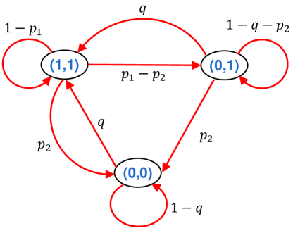
Figure 7: The transitions of the Markov chain $\{(z_{k},\tilde{z}_{k})\}_{k\in\mathbb{N}}$ when $p_{2}+q\leq 1$.

Appendix F. Proof of Theorem 4

Let $p=p_{c}(q)$ be the critical value established in Proposition 2. For any given $p$, fix a $1-1/|\lambda_{A}|^{2}<q_{1}<1$ so that $\sup_{k\in\mathbb{N}}\mathbb{E}_{q_{1}}\|P_{k}\|<\infty$ for all $\Sigma_{0}\geq 0$. From a symmetrical coupling argument as the proof of Proposition 2, for any $q_{1}\leq q_{2}<1$, $\sup_{k\in\mathbb{N}}\mathbb{E}_{q_{2}}\|P_{k}\|<\infty$ also holds for all $\Sigma_{0}\geq 0$. As a result, $p_{c}(q)$ is a non-decreasing function of $q$.

Consequently, $p_{c}(\cdot)$ yields an inverse function, denoted $q_{c}(\cdot)$, which is also non-decreasing. The desired conclusion then follows immediately, e.g., we can simply choose $f_{c}(p,q)=p_{c}(q)-p$.

Appendix G. Proof of Theorem 5

We shall first show that

$$\lim_{\eta\rightarrow 1^{+}}{p}(\eta)=\underline{p}$$ (39)

holds where $\eta>1$ is properly taken so that $\eta^{2}|\lambda_{A}|^{2}(1-q)<1$, and

$${p}(\eta)\triangleq\sup\big{\{}p:\exists(K,P)\hbox{\leavevmode\nobreak\ s.t.\leavevmode\nobreak\ }\mathcal{L}(\eta A,K,P,p)<P,P>0\big{\}}$$

with the notation $\mathcal{L}(A,K,P,p)$ used to alter $\mathcal{L}_{K}(P)$ in the proof so as to emphasize the relevance of $\mathcal{L}_{K}(P)$ to $A$ and $p$. To this end, first note that ${p}(\eta)$ is a non-increasing function of $\eta$. Thus, $\lim_{\eta\rightarrow 1^{+}}{p}(\eta)$ must exist. To show the equality in (39), we require the following lemma.

Lemma 12

Suppose $X,\tilde{X}>0$ are the solutionis to the following Lyapunov equations respectively:

$$X=(1-q)AXA^{\prime}+\tilde{Q},\leavevmode\nobreak\ \leavevmode\nobreak\ \leavevmode\nobreak\ \eta^{-1}\tilde{X}=(1-q)A\tilde{X}A^{\prime}+\tilde{Q},$$

where $\tilde{Q}>0$, $0<q<1$ and $\eta>1$ are properly taken so that $\eta(1-q)|\lambda_{A}|^{2}<1$. Then, for any $\epsilon>0$ there always exists a $\delta>0$ such that $\eta\leq 1+\delta$ implies $\tilde{X}\leq(1+\epsilon)X.$

Proof. First we shall find an upper bound for $X$ and a lower bound for $\tilde{X}$. It is straightforward that

$$X\geq\tilde{Q}\geq\|{\tilde{Q}}^{-1}\|^{-1}I.$$ (40)

Let $d\triangleq\left[{(1-q)|\lambda_{A}|^{2}}\right]^{-{1}/{4}}>1$ and restrict $1<\eta\leq d$. By Lemma 5, we have

$$\tilde{X} = \sum_{i=0}^{\infty}\eta^{i}(1-q)^{i}A^{i}\tilde{Q}(A^{i})^{\prime}$$

$$\leq \|\tilde{Q}\|\sum_{i=0}^{\infty}\eta^{i}(1-q)^{i}\|A^{i}\|^{2}I$$

$$\leq n\|\tilde{Q}\|(1+2/\varepsilon)^{2n-2}\sum_{i=0}^{\infty}d^{i}(1-q)^{i}(|\lambda_{A}|+\varepsilon\|A\|)^{2i}I$$

for any $\varepsilon>0.$ Taking $\varepsilon=\frac{(d-1)|\lambda_{A}|}{\|A\|}$, it yields that $\tilde{X}\leq\frac{cd}{d-1}\|\tilde{Q}\|$ with $c=n(1+2/\varepsilon)^{2n-2}$. Note that $\tilde{X}-X$ is bounded in the following way

$$\tilde{X}-X = \eta(1-q)A\tilde{X}A^{\prime}+\eta\tilde{Q}-(1-q)AXA^{\prime}-\tilde{Q}$$

$$= (1-q)A(\tilde{X}-X)A^{\prime}+(\eta-1)\left[(1-q)A\tilde{X}A^{\prime}+\tilde{Q}\right]$$

$$\leq (1-q)A(\tilde{X}-X)A^{\prime}+(\eta-1)\tilde{X}$$

$$\vdots$$

$$\leq (1-q)^{k}A^{k}(\tilde{X}-X)(\cdot)^{\prime}+(\eta-1)\sum_{i=0}^{k-1}(1-q)^{i}A^{i}\tilde{X}(A^{i})^{\prime}$$

Taking limitation on both sides, we obtain that $\tilde{X}-X\leq(\eta-1)\sum_{i=0}^{\infty}(1-q)^{i}A^{i}\tilde{X}(A^{i})^{\prime}$, which by Lemma 5 and (40) gives

$$\tilde{X}-X \leq (\eta-1)\|\tilde{Q}\|\frac{cd}{d-1}\sum_{i=0}^{\infty}(1-q)^{i}\|A^{i}\|^{2}\,I$$

$$\leq \frac{c^{2}d^{3}}{(d^{2}-1)(d-1)}(\eta-1)\|\tilde{Q}\|\,I$$

$$\leq \frac{c^{2}d^{3}}{(d^{2}-1)(d-1)}(\eta-1)\|\tilde{Q}\|\|{\tilde{Q}}^{-1}\|\,X$$

where the last inequality holds because of (40). Due to the positive definiteness of $\tilde{Q}$, the assertion follows by letting

$$1<\eta\leq\min\left\{\frac{(d^{2}-1)(d-1)}{c^{2}d^{3}\|\tilde{Q}\|\|{\tilde{Q}}^{-1}\|}\epsilon+1,d\right\}.$$

$\square$

By the definition of $\underline{p}$ one can verify that for any $0<\varepsilon<\underline{p}$ there always exists at least a $p\in(\underline{p}-\varepsilon,\underline{p})$ so that there exist $K$ and $P>0$ satisfying $\mathcal{L}(A,K,P,p)<P$; otherwise it contradicts (14). We take an $\epsilon>0$ so that $(1+\epsilon)\mathcal{L}(A,K,P,p)<P$ still holds. Then, from Lemma 12, there always exists an $\eta_{0}>1$ satisfying $\Phi_{\eta_{0}}\leq\sqrt{1+\epsilon}\Phi$ where $\Phi$ and $\Phi_{\eta_{0}}$ are the positive definite solutions to the following equations respectively:

$$\Phi=(1-q)A^{\prime}\Phi A+A^{\prime}PA,\leavevmode\nobreak\ \leavevmode\nobreak\ \leavevmode\nobreak\ \eta_{0}^{-2}\Phi_{\eta_{0}}=(1-q)A^{\prime}\Phi_{\eta_{0}}A+A^{\prime}PA.$$

In addition, there exists an $\eta_{1}>1$ such that $\eta_{1}^{2\mathsf{I_{o}}-2}\leq\sqrt{1+\epsilon}.$ Letting $\tilde{\eta}=\min\{\eta_{0},\eta_{1}\}$, we have

$$P>(1+\epsilon)\mathcal{L}(A,K,P,p)\geq p\sum_{i=1}^{\mathsf{I_{o}}-1}(1-p)^{i-1}(\tilde{\eta}^{i}A^{i}+\tilde{\eta}^{i}K^{(i)}C^{(i)})^{*}(\Phi_{\tilde{\eta}})(\tilde{\eta}^{i}A^{i}+\tilde{\eta}^{i}K^{(i)}C^{(i)}),$$

which implies that $\mathcal{L}(\tilde{\eta}A,K_{\tilde{\eta}},P,p)<P$ with $K_{\tilde{\eta}}\triangleq[\tilde{\eta}K^{(1)},\ldots,\tilde{\eta}^{\mathsf{I_{o}}-1}K^{(\mathsf{I_{o}}-1)}]$ and therefor that ${p}(\tilde{\eta})>\underline{p}-\varepsilon$. As $\varepsilon$ is any positive real number, $\lim_{\eta\rightarrow 1^{+}}{p}(\eta)=\underline{p}$ consequently holds. Since $\eta A$ has no defective eigenvalues on the unit circle, combining Theorems 2 and 3, we obtain that $p_{c}(\eta A,C,q)\geq{p}(\eta)$ holds.

To conclude, we also need to establish the following lemma.

Lemma 13

For a given recovery rate $q$ satisfying $|\lambda_{A}|^{2}(1-q)<1$, denote $q_{c}(A,C,q)$ as the critical value of $q_{c}$ for a system $(C,A)$. Then, we have

$$p_{c}(A,C,q)\geq\lim_{\eta\rightarrow 1^{+}}p_{c}(\eta A,C,q).$$ (41)

Proof. To emphasize the relevance of $h(X)$ and $g(X)$ to $A$, we will change the notations $h(X)$ and $g(X)$ into $h(A,X)$ and $g(A,X)$ respectively in the proof. Note that $h(\eta A,X)$ and $g(\eta A,X)$ are both non-decreasing function of $\eta>1$, where $\eta$ is properly chosen so that $\eta^{2}|\lambda_{A}|^{2}(1-q)<1$, since, for all $1\leq\eta_{1}\leq\eta_{2}\leq 1+\delta$ and $X\geq 0$, one has

$$h(\eta_{2}A,X)-h(\eta_{1}A,X)=(\eta_{2}^{2}-\eta_{1}^{2})AXA^{\prime}\geq 0$$

and

$$g(\eta_{2}A,X)-g(\eta_{1}A,X)=(\eta_{2}^{2}-\eta_{1}^{2})(AXA^{\prime}-AXC^{\prime}(CXC^{\prime}+R)^{-1}CXA^{\prime})\geq 0.$$

According to the fact that $P_{k}=(1-\gamma_{k})h(A,P_{k-1})+\gamma_{k}g(A,P_{k-1})$ and that $h(A,X)$ and $g(A,X)$ are non-decreasing functions of $X$ from Lemma 3, we can easily show by induction that $P_{k}$ is also non-decreasing with respect to $\eta$. Therefore the limitation on the right side of (41) always exists and then the conclusion follows. $\square$

From Lemma 13 and what has been proved previously, it can be seen that $\lim_{\eta\rightarrow 1^{+}}p_{c}(\eta A,C,q)$ and $\lim_{\eta\rightarrow 1^{+}}{p}(\eta)$ exist and moreover that

$$p_{c}(A,C,q)\geq\lim_{\eta\rightarrow 1^{+}}p_{c}(\eta A,C,q)\geq\lim_{\eta\rightarrow 1^{+}}{p}(\eta)=\underline{p},$$

whereby the desired result follows.

Junfeng Wu and Karl H. Johansson
ACCESS Linnaeus Centre, School of Electrical Engineering, KTH Royal Institute of Technology,
Stockholm 100 44, Sweden
Email: junfengw@kth.se, kallej@kth.se

Guodong Shi and Brian D. O. Anderson
College of Engineering and Computer Science, The Australian National University,
Canberra, ACT 0200 Australia
Email: guodong.shi@anu.edu.au, brian.anderson@anu.edu.au

References

- [1] D. F. Delchamps, “Stabilizing a linear system with quantized state feedback,” IEEE Transactions on Automatic Control, vol. 35, pp. 916–924, 1990.
- [2] W. S. Wong and R. W. Brockett, “Systems with finite communication bandwidth-part I: State estimation problems,” IEEE Transactions on Automatic Control, vol. 42, no. 9, pp. 1294–1299, 1997.
- [3] ——, “Systems with finite communication bandwidth-part II: Stabilization with limited information feedback,” IEEE Transactions on Automatic Control, vol. 44, no. 5, pp. 1049–1053, 1999.
- [4] R. W. Brockett and D. Liberzon, “Quantized feedback stabilization of linear systems,” IEEE Transactions on Automatic Control, vol. 45, no. 7, pp. 1279–1289, 2000.
- [5] G. N. Nair and R. J. Evans, “Communication-limited stabilization of linear systems,” in Proceedings of the 39th IEEE Conference on Decision and Control, 2000, pp. 1005–1010.
- [6] S. Tatikonda and S. Mitter, “Control under communication constraints,” IEEE Transactions on Automatic Control, vol. 49, pp. 1056 – 1068, July 2004.
- [7] N. Elia and S. Mitter, “Stabilization of linear systems with limited information,” IEEE Transactions on Automatic Control, vol. 46, no. 9, pp. 1384–1400, 2001.
- [8] N. Elia, “Remote stabilization over fading channels,” System and Control Letters, vol. 54(3), pp. 237–249, March 2005.
- [9] H. Ishii and B. A. Francis, “Quadratic stabilization of sampled-data systems with quantization,” Automatica, vol. 39, pp. 1793–1800, 2003.
- [10] M. Fu and L. Xie, “The sector bound approach to quantized feedback control,” IEEE Transactions on Automatic Control, vol. 50, no. 11, pp. 1698 – 1711, 2005.
- [11] J. Hespanha, P. Naghshtabrizi, and Y. Xu, “A survey of recent results in networked control systems,” Proceedings of the IEEE, vol. 95, no. 1, pp. 138–162, 2007.
- [12] B. Sinopoli, L. Schenato, M. Franceschetti, K. Poola, M. Jordan, and S. Sastry, “Kalman filtering with intermittent observations,” IEEE Transactions on Automatic Control, vol. 49, no. 9, pp. 1453–1464, 2004.
- [13] K. Plarre and F. Bullo, “On Kalman filtering for detectable systems with intermittent observations,” IEEE Transactions on Automatic Control, vol. 54, no. 2, pp. 386–390, Feb 2009.
- [14] Y. Mo and B. Sinopoli, “Towards finding the critical value for Kalman filtering with intermittent observations,” arXiv preprint arXiv:1005.2442, 2010.
- [15] B. Sinopoli, L. Schenato, M. Franceschetti, K. Poolla, and S. S. Sastry, “Optimal control with unreliable communication: the TCP case,” in Proceedings of the American Control Conference, 2005, pp. 3354–3359.
- [16] O. C. Imer, S. Yüksel, and T. Başar, “Optimal control of LTI systems over unreliable communication links,” Automatica, vol. 42, no. 9, pp. 1429–1439, 2006.
- [17] B. Sinopoli, L. Schenato, M. Franceschetti, K. Poolla, and S. Sastry, “Optimal linear LQG control over lossy networks without packet acknowledgment,” Asian Journal of Control, vol. 10, no. 1, pp. 3–13, 2008.
- [18] L. Schenato, B. Sinopoli, M. Franceschetti, K. Poolla, and S. Sastry, “Foundations of control and estimation over lossy networks,” Proceedings of the IEEE, vol. 95, pp. 163–187, 2007.
- [19] E. N. Gilbert, “Capacity of a burst-noise channel,” Bell system technical journal, vol. 39, no. 5, pp. 1253–1265, 1960.
- [20] E. Elliott, “Estimates of error rates for codes on burst-noise channels,” Bell system technical journal, vol. 42, no. 5, pp. 1977–1997, 1963.
- [21] M. Huang and S. Dey, “Kalman filtering with Markovian packet losses and stability criteria,” in Proceedings of the 45th IEEE Conference on Decision and Control, 2006, pp. 5621–5626.
- [22] ——, “Stability of Kalman filtering with Markovian packet losses,” Automatica, vol. 43, pp. 598–607, 2007.
- [23] L. Xie and L. Xie, “Peak covariance stability of a random Riccati equation arising from Kalman filtering with observation losses,” Journal of Systems Science and Complexity, vol. 20, no. 2, pp. 262–272, 2007.
- [24] ——, “Stability of a random Riccati equation with Markovian binary switching,” IEEE Transactions on Automatic Control, vol. 53, no. 7, pp. 1759–1764, 2008.
- [25] K. You, M. Fu, and L. Xie, “Mean square stability for Kalman filtering with Markovian packet losses,” Automatica, vol. 47, no. 12, pp. 2647–2657, 2011.
- [26] L. Shi, M. Epstein, and R. M. Murray, “Kalman filtering over a packet-dropping network: A probabilistic perspective,” IEEE Transactions on Automatic Control, vol. 55, no. 9, pp. 594–604, 2010.
- [27] Y. Mo and B. Sinopoli, “Kalman filtering with intermittent observations: Tail distribution and critical value,” IEEE Transactions on Automatic Control, vol. 57, no. 3, pp. 677–689, March 2012.
- [28] S. Kar, B. Sinopoli, and J. M. Moura, “Kalman filtering with intermittent observations: Weak convergence to a stationary distribution,” IEEE Transactions on Automatic Control, vol. 57, no. 2, pp. 405–420, 2012.
- [29] A. Censi, “Kalman filtering with intermittent observations: convergence for semi-Markov chains and an intrinsic performance measure,” IEEE Transactions on Automatic Control, vol. 56, no. 2, pp. 376–381, 2011.
- [30] L. Xie, “Stochastic comparison, boundedness, weak convergence, and ergodicity of a random Riccati equation with Markovian binary switching,” SIAM Journal on Control and Optimization, vol. 50, no. 1, pp. 532–558, 2012.
- [31] R. Durrett, Probability: Theory and Examples. Cambridge university press, 2010.
- [32] R. A. Horn and C. R. Johnson, Matrix analysis. Cambridge university press, 2012.
- [33] N. Xiao, L. Xie, and M. Fu, “Kalman filtering over unreliable communication networks with bounded Markovian packet dropouts,” International Journal of Robust and Nonlinear Control, vol. 19, no. 16.
- [34] H. S. Wang and N. Moayeri, “Finite-state Markov channel-a useful model for radio communication channels,” IEEE Transactions on Vehicular Technology, vol. 44, no. 1, pp. 163–171, 1995.
- [35] Q. Zhang and S. A. Kassam, “Finite-state markov model for rayleigh fading channels,” IEEE Transactions on Communications, vol. 47, no. 11, pp. 1688–1692, 1999.
- [36] B. Sinopoli, L. Schenato, M. Franceschetti, K. Poolla, M. Jordan, and S. Sastry, “Kalman filtering with intermittent observations,” IEEE Transactions on Automatic Control, vol. 49, no. 9, pp. 1453–1464, 2004.
- [37] V. Solo, “One step ahead adaptive controller with slowly time-varying parameters,” Department of EECS, John Hopkins University, Baltimore, MD, USA, Tech. Rep., 1991.
- [38] O. L. V. Costa and M. Fragoso, “Comments on ”stochastic stability of jump linear systems”,” IEEE Transactions on Automatic Control, vol. 49, no. 8, pp. 1414–1416, Aug 2004.
- [39] P. Lancaster and L. Rodman, Algebraic Riccati equations. Oxford University Press, 1995.