Fast cooling for a system of stochastic oscillators

Abstract

We study feedback control of coupled nonlinear stochastic oscillators in a force field. We first consider the problem of asymptotically driving the system to a desired steady state corresponding to reduced thermal noise. Among the feedback controls achieving the desired asymptotic transfer, we find that the most efficient one from an energy point of view is characterized by time-reversibility. We also extend the theory of Schrödinger bridges to this model, thereby steering the system in finite time and with minimum effort to a target steady-state distribution. The system can then be maintained in this state through the optimal steady-state feedback control. The solution, in the finite-horizon case, involves a space-time harmonic function $\varphi$, and $-\log\varphi$ plays the role of an artificial, time-varying potential in which the desired evolution occurs. This framework appears extremely general and flexible and can be viewed as a considerable generalization of existing active control strategies such as macromolecular cooling. In the case of a quadratic potential, the results assume a form particularly attractive from the algorithmic viewpoint as the optimal control can be computed via deterministic matricial differential equations. An example involving inertial particles illustrates both transient and steady state optimal feedback control.

I Introduction

Stochastic oscillators represent a most fundamental model of dissipative processes since the 1908 paper by Paul Langevin Lan which appeared three years after the ground-breaking work of Einstein and Smoluchowski. These stochastic models culminated in 1928 in the Nyquist-Johnson model for RLC networks with noisy resistors and in 1930 in the Ornstein-Uhlenbeck model of physical Brownian motion N1 . In more recent times, they play a central role in cold damping feedback. The latter is employed to reduce the effect of thermal noise on the motion of an oscillator by applying a viscous-like force, which is historically one of the very first feedback control actions ever analyzed. It was first implemented in the fifties on electrometers MZV . Since then, it has been successfully employed in a variety of areas such as atomic force microscopy (AFM) LMC , polymer dynamics DE ; BBP and nano to meter-sized resonators, see FK ; MG ; SR ; Vin ; PV . These new applications also pose new physics questions as the system is driven to a non-equilibrium steady state Q ; KQ ; BCD ; PT1 . In FH , a suitable efficiency measure for these diffusion-mediated devices was introduced which involves a class of stochastic control problems.

In spite of the flourishing of these applications and cutting edge developments, the interest in these problems in the control engineering community has been shallow to say the least. However, as we argue below, these problems may be cast in the framework of a suitable extension of the classical theory of Schrödinger bridges for diffusion processes W where the time-interval is finite or infinite. Moreover, a connection between finite-horizon Schrödinger bridges and the so called “logarithmic transformation” of stochastic control of Fleming, Holland, Mitter et al., see e.g.F , has been known for some time DP ; Bl ; DPP ; PW . Excepting some special cases FH ; FHS , however, the optimal control is not provided by the theory in an implementable form and a wide gap persists between the simple constant linear feedback controls used in the laboratory and the Schrödinger bridge theory which requires the solution of two partial differential equations nonlinearly coupled through their boundary values –these coupled differential equations are known as a “Schrödinger system” W . Only recently some progress has been made in deriving implementable forms of the optimal control for general linear stochastic systems CG2014 ; CGP ; CGP_ACC15 ; CGP2 as well as implementable solutions of analogous Schrödinger systems for Markov chains, Kraus maps of statistical quantum mechanics, and for diffusion processes GP ; CGP6.15 .

In this paper, continuing the work of CG2014 ; CGP ; CGP_ACC15 ; CGP2 , we study a general system of nonlinear stochastic oscillators. For this general model, we prove optimality of certain feedback controls which are given in an explicit or computable form. We also highlight the relevance of optimal controls on examples of stochastic oscillators. In Section II we introduce the system of nonlinear stochastic oscillators and discuss a fluctuation-dissipation relation and reversibility. In Section III we discuss thoroughly the existence of invariant measures and related topics such as ergodicity and convergence to equilibrium first in the case of linear dynamics and then in the general case. In Section IV, we characterize the most efficient feedback law which achieves the desired asymptotic cooling and relate optimality to reversibility of the controlled evolution. In Section V, we show how the desired cooling can be accomplished in finite time using a suitable generalization of the theory of Schrödinger bridges. The latter results are then specialized in the following section, Section VI, to the case of a quadratic potential where the equations become linear and the results of CGP lead to implementable optimal controls. Optimal transient and steady state feedback controls are illustrated in one example involving inertial particles in Section VII.

II A system of stochastic oscillators

Consider a mechanical system in a force field coupled to a heat bath. More specifically, consider the following generalization of the Ornstein-Uhlenbeck model of physical Brownian motion N1

$$dx(t) = v(t)\,dt,\quad x(t_{0})=x_{0}\;{\rm a.s.}$$ (1a)

$$Mdv(t) = -Bv(t)\,dt-\nabla_{x}V(x(t))dt+\Sigma dW(t),\quad v(t_{0})=v_{0}\;{\rm a.s.}$$ (1b)

that was also studied in HP1 . Here $x(t)$ and $v(t)$ take values in $\mathbb{R}^{n}$ where $n=3N$ and $N$ is the number of oscillators. The potential $V\in C^{1}$ (i.e., continuously differentiable), is bounded below and tends to infinity for $\|x\|\rightarrow\infty$. The noise process $W(\cdot)$ is a standard $n$-dimensional Wiener process independent of the pair $(x_{0},v_{0})$. The matrices $M$, $B$ and $\Sigma$ are $n\times n$ with $M$ symmetric and positive definite, and $\Sigma$ nonsingular. We also assume throughout the paper that $B+B^{\prime}$, where ^′ denotes the transposition, is positive semi-definite.

The one-time phase space probability density $\rho_{t}(x,v)$, or more generally probability measure $\mu_{t}(x,v)$, represents the state of the thermodynamical system at time $t$. Notice that we allow for both potential and dissipative interaction among the particles/modes, with velocity coupling and with dissipation described by a linear law. The models that will be discussed in Section V are more special and correspond to the situation where $M$, $B$ and $\Sigma$ are in fact diagonal matrices. Other spatial arrangements and interaction patterns may be accommodated in this frame as, for instance, a ring of $N$-oscillators with $x_{0}=x_{N}$ described by the scalar equations

$$dx_{k} = v_{k}dt,$$ (2a)

$$m_{k}dv_{k} = \left(-\gamma v_{k-1}-\beta v_{k}-\gamma v_{k+1}-\frac{\partial V(x)}{\partial x_{k}}\right)dt+\sigma_{k}dW,$$ (2b)

where $\sigma_{k}\in\mathbb{R}^{1\times n}$, cf. (HP1, , Section 6). For this case, (2) can be put in the form (1) by defining

$$M=\mathop{\mathrm{diag}}(m_{1},\ldots,m_{N}),\quad B=\left(\begin{matrix}\beta&\gamma&0&0&\cdot&\gamma\\ \gamma&\beta&\gamma&0&\cdot&0\\ 0&\gamma&\beta&\gamma&\cdot&0\\ 0&0&\gamma&\beta&\cdot&\cdot\\ \cdot&\cdot&\cdot&\cdot&\cdot&\gamma\\ \gamma&\cdot&\cdot&\cdot&\gamma&\beta\end{matrix}\right),\quad\Sigma=\left(\begin{matrix}\sigma_{1}\\ \cdot\\ \cdot\\ \cdot\\ \sigma_{N}\end{matrix}\right).$$

Besides thermodynamics, applications of this basic model of dissipative processes is found in nonlinear circuits with noisy resistors, in chemical physics, in biology, and other fields, e.g., see TW ; LE ; RS .

II.1 Boltzmann’s distribution and a fluctuation-dissipation relation

According to the Gibbsian postulate of classical statistical mechanics, the equilibrium state of a system in contact with a heat bath at constant absolute temperature $T$ and with Hamiltonian function $H$ is necessarily given by the Boltzmann distribution law

$$\rho_{B}=Z^{-1}\exp\left[-\frac{H}{kT}\right]$$ (3)

where $Z$ is the partition function. The Hamiltonian function corresponding to (1) is

$$H(x,v)=\frac{1}{2}\langle v,Mv\rangle+V(x),$$

where $\langle\cdot,\cdot\rangle$ denotes the Euclidean scalar product in $\mathbb{R}^{n}$; the partition function is simply a normalization constant.

The key mathematical concept relevant to a stochastic characterization of equilibrium is that of an invariant probability measure. However, not all invariant probability measures correspond to equilibrium. They may represent a steady state of nonequilibrium thermodynamics. Thus, while it is important to establish existence and uniqueness of the invariant probability measure, it is also necessary to characterize when we can expect such a measure to be of the Boltzmann-Gibbs type (3). For the system of stochastic oscillators (1), this was established in HP1 , generalizing the Einstein fluctuation-dissipation relation:

Proposition 1

An invariant measure for (1) is a Boltzmann distribution with density (3) if and only if

$$\Sigma\Sigma^{\prime}=kT(B+B^{\prime}).$$ (4)

Before dealing with existence of invariant measures, we discuss reversibility.

II.2 Reversibility

Let us start recalling that a stochastic process $\{X(t),t\in T\}$ taking values in $\cal X$ and with the invariant measure $\bar{\mu}$ is called reversible if its finite dimensional distributions coincide with those of the time-reversed process. Namely, for all $t_{1}<t_{2}<\cdots<t_{m}$ and $x_{i}\in{\cal X}$,

$$\mathbb{P}_{\bar{\mu}}(X(t_{1})=x_{1},X(t_{2})=x_{2},\ldots,X(t_{n})=x_{n})=\mathbb{P}_{\bar{\mu}}(X(t_{1})=x_{n},X(t_{2})=x_{n-1},\ldots,X(t_{n})=x_{1}).$$

For a Markov-diffusion process such as (1), it should be possible to characterize reversibility through the stochastic differentials. Indeed, it has been shown by Nelson N1 ; N2 , see also HP , that Markov diffusion processes admit, under rather mild conditions, a reverse-time stochastic differential. For (1), this stochastic differential takes the form

$$dx(t) = v(t)\,dt,$$ (5a)

$$Mdv(t) = -Bv(t)\,dt-\nabla_{x}V(x(t))dt-\Sigma\Sigma^{\prime}M^{-1}\nabla_{v}\log\rho_{t}(x(t),v(t))+\Sigma dW_{-}(t).$$ (5b)

Here $dt>0$, $\rho_{t}$ is the probability density of the process in phase space, and $W_{-}$ is a standard Wiener process whose past $\{W_{-}(s);0\leq s\leq t\}$ is independent of $\left(\begin{matrix}x(t)\\ v(t)\end{matrix}\right)$ for all $t\geq 0$.

Consider now the situation where $\rho_{t}(x,v)=\bar{\rho}(x,v)$ an invariant density. Consider also the time reversal transformation Gu

$$t\rightarrow t^{\prime}=-t,\quad x\rightarrow x^{\prime}=x,\quad v\rightarrow v^{\prime}=-v,\quad\nabla_{x}\rightarrow\nabla_{x^{\prime}}=\nabla_{x},\quad\nabla_{v}\rightarrow\nabla_{v^{\prime}}=-\nabla_{v}.$$

In view of (1b) and (5b), we also define

$$F_{+}(x,v,t)=-Bv-\nabla_{x}V(x),\quad F_{-}(x,v,t)=-Bv-\nabla_{x}V(x)-\Sigma\Sigma^{\prime}M^{-1}\nabla_{v}\log\bar{\rho}(x,v).$$

Then, we have invariance under time reversal if and only if

$$F_{+}^{\prime}(x^{\prime},v^{\prime},t^{\prime})=F_{-}(x,v,t)=-Bv-\nabla_{x}V(x)-\Sigma\Sigma^{\prime}M^{-1}\nabla_{v}\log\bar{\rho}(x,v)$$

$$=F_{+}(x^{\prime},v^{\prime},t^{\prime})=-Bv^{\prime}-\nabla_{x^{\prime}}V(x^{\prime})=Bv-\nabla_{x}V(x).$$

We get the condition

$$\Sigma\Sigma^{\prime}M^{-1}\nabla_{v}\log\bar{\rho}(x,v)=-2Bv.$$ (6)

We have therefore the following result.

Proposition 2

The phase-space process (1) with the invariant Boltzmann distribution (3) is reversible if and only if the matrix $B$ is symmetric positive definite.

Proof. Since $\nabla_{v}\log\rho_{B}(x,v)=-\frac{1}{kT}Mv$, (6) reads

$$\frac{1}{kT}\Sigma\Sigma^{\prime}v=2Bv,\quad v\in\mathbb{R}^{n}.$$

which holds true if and only if $B$ is symmetric positive definite ($\Sigma$ is nonsingular) satisfying (4), namely

$$\Sigma\Sigma^{\prime}=2kTB.$$ (7)

$\Box$ In (HP1, , Proposition 2.1), it was shown that, under (4), symmetry of $B$ is a necessary and sufficient condition for a Newton-type law to hold. The latter can be derived from a Hamilton-like principle in analogy to classical mechanics P . In the next section, we deal in some detail with the issue of existence and properties of an invariant measure for (1).

III Invariant measures for the system of stochastic oscillators

This topic is in general a rather delicate one and the mathematical literature covering model (1) is rather scarce. We have therefore decided to give a reasonably comprehensive account of the issues and results. We discuss first the case of a quadratic potential where the dynamics becomes linear and simple linear algebra conditions may be obtained. This case is also of central importance for cooling applications LMC ; DE ; Vin .

III.1 Invariant measures: The case of a quadratic potential function

We assume in this subsection that

$$V(x)=\frac{1}{2}\langle x,Kx\rangle$$

with $K$ symmetric positive definite so that the various restoring forces in the vector Langevin equation (1) are linear and the system takes the form:

$$d\xi={\cal A}\xi dt+{\cal B}dW(t)$$ (8a)

where

$$\xi=\left(\begin{matrix}x\\ v\end{matrix}\right),\quad\cal A=\left(\begin{matrix}0&I\\ -M^{-1}K&-M^{-1}B\end{matrix}\right),\quad\cal B=\left(\begin{matrix}0\\ M^{-1}\Sigma\end{matrix}\right).$$ (8b)

This case has been thoroughly studied in (HP1, , Section 5) building on the deterministic results of Müller Mu and Wimmer Wim . Thus, we only give below the essential concepts and results for the sake of continuity in exposition.

As is well known FCG , the existence of a Gaussian invariant measure with nonsingular covariance matrix ${\cal P}$ is intimately connected to the existence of a positive definite ${\cal P}$ satisfying the Lyapunov equation

$$0=\cal A\cal P+\cal P\cal A^{\prime}+\cal B\cal B^{\prime}.$$ (9)

Inertia theorems for (9) Wim relate the spectrum of ${\cal P}$ to the spectrum of ${\cal A}$ and controllability of an associated deterministic system. Recall that for a dynamical system

$$\dot{\xi}(t)=f(\xi(t),u(t),t),\quad\xi(0)=\xi_{0}$$

(complete) controllability refers to the property of an external input (the vector of control variables $u(t)$) to steer the internal state $\xi(t)$ in finite time from any initial condition $\xi_{0}$ to any desired target state. It turns out that the pair $({\cal A},{\cal B})$ gives rise to a controllable linear system

$$\dot{\xi}(t)={\cal A}\xi(t)+{\cal B}u(t)$$

if and only if the matrix $({\cal B},{\cal A}{\cal B},\ldots,{\cal A}^{2n-1}{\cal B})$ has full row rank KFA . Now, suppose $\cal P$ is positive definite and satisfies (9). Let $\lambda$ be an eigenvalue of $\cal A^{\prime}$ with $\gamma$ a corresponding eigenvector. Then

$$0=\gamma^{\prime}\left[\cal A\cal P+\cal P\cal A^{\prime}+\cal B\cal B^{\prime}\right]\gamma=(\lambda+\bar{\lambda})\gamma^{\prime}\cal P\gamma+\gamma^{\prime}\cal B\cal B^{\prime}\gamma.$$

Since $\gamma^{\prime}{\cal P}\gamma>0$ and $\gamma^{\prime}{\cal B}{\cal B}^{\prime}\gamma\geq 0$, it follows that $\Re[\lambda]\leq 0$. That is, the spectrum of ${\cal A}$ is contained in the left half of the complex plane. In the other direction, if ${\cal A}$ is asymptotically stable (i.e., all eigenvalues are in the open left half-plane), $\cal P$ given by

$${\cal P}=\int_{0}^{\infty}e^{{\cal A}\tau}{\cal B}{\cal B}^{\prime}e^{{\cal A}^{\prime}\tau}d\tau$$

satisfies (9) and is positive semidefinite –this is the so-called controllability Gramian. It turns out that this is positive definite if and only if the pair $({\cal A},{\cal B})$ is controllable FCG .

For $({\cal A},{\cal B})$ as in (8b) and under the present assumptions ($\Sigma$ nonsingular), the matrix $({\cal B},{\cal A}{\cal B},\ldots,{\cal A}^{2n-1}{\cal B})$ always has full row rank. Thus, existence and uniqueness of a nondegenerate Gaussian invariant measure is reduced to characterizing asymptotic stability of the matrix ${\cal A}$ in (8b). When ${\cal A}$ is asymptotically stable, starting from any initial Gaussian distribution, we have convergence to the invariant Gaussian density with zero mean and covariance ${\cal P}$. Asymptotic stability of ${\cal A}$ can be studied via stability theory for the deterministic system

$$M\ddot{z}(t)+\frac{B+B^{\prime}}{2}\dot{z}(t)+Kz(t)=0$$

employing as Lyapunov function the energy $H(x,v)=\frac{1}{2}\langle v,Mv\rangle+\frac{1}{2}\langle x,Kx\rangle$. In the case when $B+B^{\prime}$ is positive semidefinite, using invariance of controllability under feedback, the asymptotic stability of ${\cal A}$ was shown by Müller Mu to be equivalent to the complete controllability of the system

$$M\ddot{z}(t)+Bu(t)+Kz(t)=0.$$ (10)

In Müller’s terminology, as quoted in Wim , this means that damping in the corresponding deterministic system is pervasive. We collect all these findings in the following theorem.

Theorem 1

Mu ; Wim In model (1), assume that $M=M^{\prime}>0$, $V(x)=\frac{1}{2}\langle x,Kx\rangle$ with $K=K^{\prime}>0$. Suppose moreover that $(B+B^{\prime})\geq 0$ and that $\Sigma$ is nonsingular. Then there exists a unique nondegenerate invariant Gaussian measure if and only if the pair of matrices

$$\left(\left[\begin{matrix}0&I\\ -M^{-1}K&0\end{matrix}\right],\left[\begin{matrix}0&0\\ 0&-M^{-1}\frac{B+B^{\prime}}{2}\end{matrix}\right]\right)$$ (11)

is controllable. In particular, this is always the case when $B+B^{\prime}$ is actually positive definite. If the invariant measure exists, it is of the Boltzmann type (3) if and only if the generalized fluctuation-dissipation relation (4) holds.

Some extensions of this result to the case of a non quadratic potential have been presented in (BM, , Section 3B).

III.2 Invariant measures: The case of a general potential function

Consider now the general case where the potential function $V$ is any nonnegative, continuously differentiable function which tends to infinity for $\|x\|\rightarrow\infty$. As already observed, existence, uniqueness, ergodicity, etc. of an invariant probability measure are quite delicate issues and we refer to the specialized literature for the full story, see e.g. (St, , Section 7.4), (DaPrato, , Chapters 5 and 7). One way to prove existence of an invariant measure is by establishing that the flow of one-time marginals $\mu_{t}(x_{0},v_{0})$, $t\geq 0$ of the random evolution in (1) starting from the point $(x_{0},v_{0})$ is tight. If that is the case, existence of an invariant measure follows from the Krylov-Bogoliubov theorem (DaPrato, , Section 7.1). One way to establish tightness of the family $\mu_{t}(x_{0},v_{0}),t\geq 0$ is via Lyapunov functions. One has, for instance, the following result.

Proposition 3

(DaPrato, , Proposition 7.10) Let ${\cal V}:\mathbb{R}^{2n}\rightarrow[0,+\infty]$ be a Borel function whose level sets $K_{a}=\{(x,v)\in\mathbb{R}^{2n}:{\cal V}(x,v)\leq a\}$ are compact for all $a>0$. Suppose there exists $(x_{0},v_{0})\in\mathbb{R}^{2n}$ and $C(x_{0},v_{0})>0$ such that the corresponding solution $(x(t,x_{0}),v(t,v_{0}))$ of (1) starting from $(x_{0},v_{0})$ is such that

$${\mathbb{E}}\{{\cal V}(x(t,x_{0}),v(t,v_{0}))\}\leq C(x_{0},v_{0}),\quad\forall t\geq 0.$$ (12)

Then, there exists an invariant measure for (1).

The natural Lyapunov function for our model is the Hamiltonian $H(x,v)$ which, under the present assumptions on the potential function $V$, does have compact level sets. Thus, we now consider the evolution of $H(x(t),v(t))$ along the random evolution of (1). By Ito’s rule KS , we get

$$dH(x(t),v(t)) = \left[\frac{\partial H}{\partial t}+\left(\begin{matrix}v(t)\\ \left(-M^{-1}Bv(t)-M^{-1}\nabla_{x}V(x(t)\right)\end{matrix}\right)\cdot\left(\begin{matrix}\nabla_{x}H\\ \nabla_{v}H\end{matrix}\right)\right.$$ (13)

$$\left.+\frac{1}{2}\sum_{i,j=1}^{n}\left[M^{-1}\Sigma\Sigma^{\prime}M^{-1}\right]_{ij}\frac{\partial^{2}H}{\partial v_{i}\partial v_{j}}\right](x(t),v(t))dt$$

$$+\nabla_{v}H(x(t),v(t))\cdot M^{-1}\Sigma dW(t)$$

$$= -\langle Bv(t),v(t)\rangle dt+\frac{1}{2}\operatorname{\rm trace}\left[M^{-1}\Sigma\Sigma^{\prime}\right]dt+v(t)^{\prime}\Sigma dW(t).$$

Let $U(t)={\mathbb{E}}\{H(x(t),v(t))\}$ be the internal energy. Then from (13), observing that $\langle Bv,v\rangle=\langle B^{\prime}v,v\rangle$, we get

$$U(t+h)-U(t)={\mathbb{E}}\left\{\int_{t}^{t+h}-\left\langle\frac{B+B^{\prime}}{2}v(\tau),v(\tau)\right\rangle d\tau\right\}+\frac{h}{2}\operatorname{\rm trace}\left[M^{-1}\Sigma\Sigma^{\prime}\right].$$ (14)

The first term represents the work done on the system by the friction forces, whereas the second is due to the action of the thermostat on the system and represents the heat, so that (14) appears as an instance of the first law of thermodynamics

$$\Delta U=W+Q.$$

Since the friction force is dissipative ($B+B^{\prime}\geq 0$), we have that $W\leq 0$. If we take $(0,0)$ as initial condition for (1), the initial variance will be zero and therefore by (14) the internal energy will initially increase. The statement that it remains bounded, so that we can apply Proposition 3, rests on the possibility that the $L^{2}$ norm of $v(\tau)$, suitably weighted by the symmetric part of the friction matrix $B$, becomes eventually at least as large as the constant quantity $\operatorname{\rm trace}\left[M^{-1}\Sigma\Sigma^{\prime}\right]$.

In the rest of this section, we discuss the case where the generalized fluctuation-dissipation relation (4) holds. Then, a direct computation on the Fokker-Planck equation associated to (1)

$$\frac{\partial{\rho}}{\partial{t}}+v\cdot\nabla_{x}\rho-\nabla_{v}\cdot\left(M^{-1}Bv+M^{-1}\nabla_{x}V\rho\right)=\frac{1}{2}\sum_{i,j=1}^{n}\left[M^{-1}\Sigma\Sigma^{\prime}M^{-1}\right]_{ij}\frac{\partial^{2}}{\partial v_{i}\partial v_{j}}\rho$$ (15)

shows that the Boltzmann density (3)

$$\rho_{B}(x,v)=Z^{-1}\exp\left[-\frac{H(x,v)}{kT}\right]=Z^{-1}\exp\left[-\frac{\frac{1}{2}\langle v,Mv\rangle+V(x)}{kT}\right]$$

is indeed invariant. We now discuss uniqueness, ergodicity and convergence of $\rho_{t}$ to $\rho_{B}$. Consider the free energy functional

$$F(\rho_{t})=kT\int_{\mathbb{R}^{n}}\int_{\mathbb{R}^{n}}\log\frac{\rho_{t}}{\rho_{B}}\rho_{t}\,dxdv=kT\,{\mathbb{D}}(\rho_{t}\|\rho_{B}),$$

where ${\mathbb{D}}(\rho\|\sigma)$ is the relative entropy or divergence or Kullback-Leibler pseudo-distance between the densities $\rho$ and $\sigma$. We have the well known result, see e.g. Gr :

$$\frac{d}{dt}F(\rho_{t})=-\frac{kT}{2}\int_{\mathbb{R}^{n}}\int_{\mathbb{R}^{n}}\langle\Sigma\Sigma^{\prime}\nabla_{v}\log\frac{\rho_{t}}{\rho_{B}},\nabla_{v}\log\frac{\rho_{t}}{\rho_{B}}\rangle\rho_{t}\,dxdv$$ (16)

Recalling that ${\mathbb{D}}(\rho\|\sigma)\geq 0$ and ${\mathbb{D}}(\rho\|\sigma)=0$ if and only if $\rho=\sigma$ Ku , we see that $F$ acts as a natural Lyapunov function for (15). The decay of $F(\rho_{t})$ implies uniqueness of the invariant density $\rho_{B}$ in the set $\{\rho|{\mathbb{D}}(\rho\|\rho_{B})<\infty\}$. Suppose now that $V$ is actually $C^{\infty}$. Then the generator (KS ) of (1), taking $M=\Sigma\Sigma^{\prime}=I$ to simplify the writing,

$$v\cdot\nabla_{x}-Bv\cdot\nabla_{v}-\nabla_{x}V\cdot\nabla_{v}+\frac{1}{2}\Delta_{v}$$ (17)

is actually hypoelliptic Bell . Indeed it can be written in Hörmander’s form

$$X_{0}+Y+\frac{1}{2}\sum_{i=1}^{n}X_{i}^{2}$$

where

$$X_{0}=-Bv\cdot\nabla_{v},\quad Y=-\nabla_{x}\cdot\nabla_{v}+v\cdot\nabla_{x},\quad X_{i}=\frac{\partial}{\partial v_{i}}.$$

Moreover, the vectors

$$(X_{1},\ldots,X_{n},[Y,X_{1}],\ldots,[Y,X_{n}])$$

form a basis of $\mathbb{R}^{2n}$ at every point (Bau, , Section 2). This is Hörmander’s condition Ho which, in the case of a quadratic potential, turns into controllability of the pair $({\cal A},{\cal B})$ in (8a). It follows that, for any initial condition $\rho_{0}$ (even a Dirac delta) the correspondig solution $\rho_{t}$ of (15) is smooth and supported on all of $\mathbb{R}^{2n}$ for all $t>0$. Let $p(s,\xi,t,\eta)$ denote the (smooth) transition density and consider the Markov semigroup

$$P_{t}[\varphi](\xi)=\int p(0,\xi,t,\eta)\varphi(\eta)d\eta,$$

for $\varphi$ a Borel bounded function on $\mathbb{R}^{2n}$. Then the Markov semigroup is regular (DaPrato, , Definition 7.3) and the invariant measure $\rho_{B}(x,v)dxdv$ is unique (DaPrato, , Proposition 7.4). This invariant measure being unique, it is necessarily ergodic (DaPrato, , Theorem 5.16) (time averages converging to probabilistic averages).

We finally turn to the convergence of $\rho_{t}$ to $\rho_{B}$. In view of (16), it seems reasonable to expect that $\rho_{t}(x,v)$ tends to $\rho_{B}(x,v)$ in relative entropy and, consequently, in $L^{1}$ (total variation of the measures) LC . This, however, does not follow from (16) and turns out to be surprisingly difficult to prove. Indeed, the result rests on the possibility of establishing a logarithmic Sobolev inequality (LSI) Le ; Bau , (Vil, , Section 9.2), a topic which has kept busy some of the finest analysts during the past forty years. One says the probability measure $\mu$ satisfies a (LSI) with constant $\lambda>0$ if for every function $f$ satisfying $\int f^{2}d\mu=1$,

$$\int f^{2}\log f^{2}d\mu\leq\frac{1}{2\lambda}\int\|\nabla f\|^{2}d\mu.$$ (18)

Let us consider a non degenerate diffusion process $\{X(t);t\geq 0\}$ taking values in some Euclidean space $\mathbb{R}^{m}$ with differential

$$dX(t)=-\frac{1}{2}\nabla R(X(t))dt+dW(t),$$

where $R$ is a smooth, nonnegative function such that $\exp[-R(x)]$ is integrable over $\mathbb{R}^{m}$. Then $\rho_{\infty}(x)=C\exp[-R(x)]$ is an invariant density for $X(t)$ where $C$ is a normalizing constant. Let $\rho_{t}$ be the one-time density of $X(t)$. Then, in analogy to (16), we have the decay of the relative entropy

$$\frac{d}{dt}{\mathbb{D}}(\rho_{t}\|\rho_{\infty})=-\frac{1}{2}\int\|\nabla\log\frac{\rho_{t}}{\rho_{\infty}}\|^{2}\rho_{t}dx.$$ (19)

The integral appearing in the right hand-side of (19) is called the relative Fisher information of $\rho_{t}$ with respect to $\rho_{\infty}$. It is also a “Dirichlet form”, as it can be rewritten as

$$4\int\|\nabla\sqrt{\frac{\rho_{t}}{\rho_{\infty}}}\|^{2}\rho_{\infty}dx,$$

see below. Suppose a LSI as in (18) holds for $\mu_{\infty}(dx)=\rho_{\infty}(x)dx$. Let $f^{2}=\rho_{t}/\rho_{\infty}$ which indeed satisfies

$$\int f^{2}d\mu=\int\frac{\rho_{t}}{\rho_{\infty}}\rho_{\infty}dx=1.$$

We then get

$${\mathbb{D}}(\rho_{t}\|\rho_{\infty})=\int\frac{\rho_{t}}{\rho_{\infty}}\log\left(\frac{\rho_{t}}{\rho_{\infty}}\right)\rho_{\infty}dx=\int f^{2}\log f^{2}d\mu\leq\frac{1}{2\lambda}\int\|\nabla f\|^{2}d\mu=$$

$$\frac{1}{2\lambda}\int\|\nabla\sqrt{\frac{\rho_{t}}{\rho_{\infty}}}\|^{2}\rho_{\infty}dx=\frac{1}{2\lambda}\int\|\nabla\log\left(\sqrt{\frac{\rho_{t}}{\rho_{\infty}}}\right)\|^{2}\rho_{t}dx=\frac{1}{8\lambda}\int\|\nabla\log\left(\frac{\rho_{t}}{\rho_{\infty}}\right)\|^{2}\rho_{t}dx$$ (20)

From (19) and (20), we finally get

$$\frac{d}{dt}{\mathbb{D}}(\rho_{t}\|\rho_{\infty})\leq-4\lambda{\mathbb{D}}(\rho_{t}\|\rho_{\infty})$$ (21)

which implies exponentially fast decay of the relative entropy to zero. Thus $\rho_{t}$ converges in the (strong) entropic sense to $\rho_{\infty}$ and therefore in $L^{1}$. Thirty years ago Bakry and Emery proved that if the function $R$ is strongly convex, i.e. the Hessian of $R$ is uniformly bounded away from zero, then $\rho_{\infty}$ satisfies a suitable LSI. This result has, since then, been extended in many ways, most noticeably by Villani Vil2 .

To establish entropic convergence of $\rho_{t}$ to $\rho_{B}$ for our degenerate diffusion model (1), we would need a suitable LSI of the form

$$\frac{1}{2}\int_{\mathbb{R}^{n}}\int_{\mathbb{R}^{n}}\langle\Sigma\Sigma^{\prime}\nabla_{v}\log\frac{\rho_{t}}{\rho_{B}},\nabla_{v}\log\frac{\rho_{t}}{\rho_{B}}\rangle\rho_{t}\,dxdv\geq 4\lambda{\mathbb{D}}(\rho_{t}\|\rho_{B}).$$

It is apparent that the possibility of establishing such a result depends only on the properties of the potential function $V$. Recently, some results in this directions have been reported in Bau under various assumptions including the rather strong one that the Hessian of $V$ be bounded.

IV Optimal steering to a steady state and reversibility

Consider again the system of stochastic oscillators (1) and let $\bar{\rho}$, given by

$$\bar{\rho}(x,v)=\bar{Z}^{-1}\exp\left[-\frac{H(x,v)}{kT_{{\rm eff}}}\right],$$ (22)

be a desired thermodynamical state with $T_{{\rm eff}}<T$, $T$ being the temperature of the thermostat. Consider the controlled evolution

$$dx(t) = v(t)\,dt,\quad x(t_{0})=x_{0}\;{\rm a.s.}$$ (23a)

$$Mdv(t) = -Bv(t)\,dt-Uv(t)dt-\nabla V(x(t))dt+\Sigma dW(t),\quad v(t_{0})=v_{0}\;{\rm a.s.},$$ (23b)

where $B$ and $\Sigma$ satisfy (4) and $U$ is a constant $n\times n$ matrix. We have the following fluctuation-dissipation relation which is a direct consequence of Proposition 1.

Corollary 1

Under condition (4), the probability density $\bar{\rho}(x,v)$ in (22) is invariant for the controlled dynamics (23) if and only if the following relation holds

$$\frac{T-T_{{\rm eff}}}{T}\Sigma\Sigma^{\prime}=kT_{{\rm eff}}\left[U+U^{\prime}\right].$$ (24)

Observe that $U$ satisfying (24) always exist. For instance, if we require $U$ to be symmetric, it becomes unique and it is explicitly given by

$$U_{{\rm sym}}=\frac{1}{2}\left[\frac{T-T_{{\rm eff}}}{kTT_{{\rm eff}}}\Sigma\Sigma^{\prime}\right].$$ (25)

Considerations on uniqueness, ergodicity and convergence are completely analogous to those of the Subsection III.2 and will not be repeated here. We shall just assume that the potential function $V$ is such that an LSI for $\bar{\rho}(x,v)dxdv$ can be established Bau leading to entropic exponential convergence of $\rho_{t}(x,v)$ to $\bar{\rho}(x,v)$ for any $U$ satisfying (24). Thus, such a control $-M^{-1}Uv$ achieves asymptotically the desired cooling.

It is interesting to investigate which of the feedback laws $-Uv$ which satisfy (24) and therefore drive the system (23) to the desired steady state $\bar{\rho}$, does it more efficiently. Following (CGP2, , Section II-B), we consider therefore the problem of minimizing the expected input power (energy rate)

$$J_{p}(u)={\mathbb{E}}\left\{u^{\prime}u\right\}$$ (26)

over the set of admissible controls

$${\mathcal{U}}_{p}=\left\{u(t)=-M^{-1}Uv(t)\mid U\mbox{ satisfies }(\ref{FD2})\right\}.$$ (27)

Observe that, under the distribution $\bar{\rho}dxdv$, $x$ and $v$ are independent. Moreover, ${\mathbb{E}}\{vv^{\prime}\}=kT_{{\rm eff}}M^{-1}$. Hence

$${\mathbb{E}}\left\{u^{\prime}u\right\}={\mathbb{E}}\left\{v^{\prime}U^{\prime}M^{-2}Uv\right\}=kT_{{\rm eff}}\operatorname{\rm trace}\left[M^{-1}U^{\prime}M^{-2}U\right].$$

We now proceed with a variational analysis that allows identifying the form of the optimal control. Let $\Pi$ be a symmetric matrix and consider the Lagrangian function

$$\mathcal{L}(U,\Pi)=kT_{{\rm eff}}\operatorname{\rm trace}\left[M^{-1}U^{\prime}M^{-2}U\right]+\operatorname{\rm trace}\left(\Pi(kT_{{\rm eff}}\left[U+U^{\prime}\right]-\frac{T-T_{{\rm eff}}}{T}\Sigma\Sigma^{\prime})\right)$$ (28)

which is a simple quadratic form in the unknown $U$. Taking variations of $U$, we get

$$\delta\mathcal{L}(U,\Pi;\delta U)=kT_{{\rm eff}}\operatorname{\rm trace}\left(\left(M^{-1}\delta U^{\prime}M^{-2}U+M^{-1}U^{\prime}M^{-2}\delta U+\Pi\delta U+\Pi\delta U^{\prime}\right)\right).$$

Setting $\delta\mathcal{L}(U,\Pi;\delta U)=0$ for all variations, which is a sufficient condition for optimality, we get $M^{-2}UM^{-1}=\Pi$ which implies that $M^{-1}U$ equals the symmetric matrix $M\Pi M$. Thus, for an extremal point $U^{*}$, we get the symmetry condition

$$U^{*}M^{-1}=M^{-1}(U^{*})^{\prime}.$$ (29)

This optimality condition can be related to reversibility in the steady state. Indeed, repeating the analysis of Subsection II.2 with $B+U$ in place of $B$, we get that the phase-space process (1) is reversible with the steady state distribution (22) if and only if

$$\Sigma\Sigma^{\prime}=2kT_{{\rm eff}}(B+U).$$

If we have reversibility in equilibrium, namely $B$ is symmetric positive definite satisfying (7), we get

$$U=\frac{T-T_{{\rm eff}}}{T_{{\rm eff}}}B=U_{{\rm sym}}>0.$$ (30)

We collect these observations in the following result.

Corollary 2

Assume $M=mI_{n}$ a scalar matrix. Then $U^{*}=U_{{\rm sym}}$. This, under the assumption that $B$ satisfies (7), is equivalent to reversibility in the steady state (22). If, morever, $B=m\beta I_{n}$ and $\Sigma=m\sigma I_{n}$, writing $T_{{\rm eff}}=(\beta/\beta+\gamma)T$, we get $U^{*}=m\gamma I$.

It follows, in particular, that what is implemented in various applications LMC ; BBP ; Vin does indeed minimize the expected control power (26) among those satisfying (24).

V Fast cooling for the system of stochastic oscillators

Consider now the same system of stochastic oscillators (1) subject to an external force represented by the control action $u(t)$:

$$dx(t) = \phantom{-}v(t)\,dt,$$ (31a)

$$Mdv(t) = -Bv(t)\,dt+u(t)dt-\nabla V(x(t))dt+\Sigma dW(t),$$ (31b)

with $x(t_{0})=x_{0}$ and $v(t_{0})=v_{0}$ a.s. Here $u$ is to be specified by the controller in order to achieve the desired cooling at a finite time $t_{1}$. That is, we seek to steer the system of stochastic oscillators to the desired steady state $\bar{\rho}$ given in (22) in finite time. Let $\mathcal{U}$ be the family of adapted, finite-energy control functions such that the initial value problem (31) is well posed on bounded time intervals and such that the probability density of the “state” process

$$\xi^{u}(t_{1})=\left(\begin{array}[]{c}x\\ v\end{array}\right)$$

is given by (22). More precisely, $u\in\mathcal{U}$ is such that $u(t)$ only depends on $t$ and on $\{\xi^{u}(s);t_{0}\leq s\leq t\}$ for each $t>t_{0}$, satisfies

$${\mathbb{E}}\left\{\int_{t_{0}}^{t_{1}}u(t)^{\prime}u(t)\,dt\right\}<\infty,$$

and is such that $\xi^{u}(t_{1})$ is distributed according to $\bar{\rho}$. The family $\mathcal{U}$ represents here the admissible control inputs which achieve the desired probability density transfer from $\rho_{0}$ to $\rho_{1}=\bar{\rho}$. Thence, we formulate the following Schrödinger Bridge Problem:

Problem 1

Determine whether ${\mathcal{U}}$ is non-empty and if so, find $u^{*}:={\rm argmin}_{u\in\mathcal{U}}\,J(u)$ where

$$J(u):={\mathbb{E}}\left\{\int_{t_{0}}^{t_{1}}\frac{1}{2}u(t)^{\prime}\left(\Sigma\Sigma^{\prime}\right)^{-1}u(t)\,dt\right\}.$$ (32)

The original motivation to study these problems comes from large deviations of the empirical distribution F2 ; ellis ; DZ , namely a rather abstract probability question first posed and, to some extent, solved by Erwin Schrödinger in two remarkable papers in 1931 and 1932 S1 ; S2 . The solution of the large deviations problem, in turn, requires solving a maximum entropy problem on path space where the uncontrolled evolution plays the role of a “prior” F2 ; W , see also PT1 ; PT2 ; GP . The latter, as we show in this specific case in Appendix A, leads to Problem 1. Observe that, after $u^{*}$ has steered the system to $\bar{\rho}$ at time $t_{1}$, we simply need to switch to a control $u(t)=-Uv(t)$, with $U$ satisfying (24), to keep the system in the desired steady state, see Section VII for an illustrating example.

To simplify the writing here and in Appendix A, we take $M=mI_{n}$, $B=m\beta I_{n}$ and $\Sigma=m\sigma I_{n}$ in (1):

$$dx(t) = v(t)\,dt,\quad x(t_{0})=x_{0}\;{\rm a.s.}$$ (33a)

$$dv(t) = -\beta v(t)\,dt-\frac{1}{m}\nabla_{x}V(x(t))dt+\sigma dW(t),\quad v(t_{0})=v_{0}\;{\rm a.s.}$$ (33b)

As we are now working on a finite time interval, the assumption that $B$ be a diagonal, positive definite matrix is not as crucial as it was in the previous two sections. Next we outline the variational analysis in the spirit of Nagasawa-Wakolbinger W to obtain a result of Jamison Jam for our degenerate diffusion (33). Let $\varphi(x,v,t)$ be any positive, space-time harmonic function for the uncontrolled evolution, namely $\varphi$ satisfies on $\mathbb{R}^{2n}\times[t_{0},t_{1}]$

$$\frac{\partial\varphi}{\partial t}+v\cdot\nabla_{x}\varphi+(-\beta v-\frac{1}{m}\nabla_{x}V)\cdot\nabla_{v}\varphi+\frac{\sigma^{2}}{2}\Delta_{v}\varphi=0.$$ (34)

It follows that $\log\varphi$ satisfies

$$\frac{\partial\log\varphi}{\partial t}+v\cdot\nabla_{x}\log\varphi+(-\beta v-\frac{1}{m}\nabla_{x}V)\cdot\nabla_{v}\log\varphi+\frac{\sigma^{2}}{2}\Delta_{v}\log\varphi=-\frac{\sigma^{2}}{2}\|\nabla_{v}\log\varphi\|^{2}.$$ (35)

Observe now that, in view of (47) in Appendix A, the maximum entropy problem is equivalent to minimizing over admissible measures $P_{u}$ on the space of paths the functional

$$I(P_{u})={\mathbb{E}}_{P_{u}}\left[\int_{t_{0}}^{t_{1}}\frac{1}{2\sigma^{2}}u\cdot udt-\log\varphi(x(t_{1}),v(t_{1}),t_{1})+\log\varphi(x(t_{0}),v(t_{0}),t_{0})\right]$$ (36)

since the endpoints marginals at $t=t_{0}$ and $t=t_{1}$ are fixed. Under $P_{u}$, by Ito’s rule KS ,

$$d\log\varphi(x(t),v(t),t) = \frac{\partial\log\varphi}{\partial t}+v\cdot\nabla_{x}\log\varphi+(-\beta v-\frac{1}{m}\nabla_{x}V+u)\cdot\nabla_{v}\log\varphi$$

$$+\frac{\sigma^{2}}{2}\Delta_{v}\log\varphi(x(t),v(t),t)dt+\nabla_{v}\log\varphi(x(t),v(t),t)\sigma dW(t).$$

Using this and (35) in (36), we now get

$$I(P_{u}) ={\mathbb{E}}_{P_{u}}\left[\int_{t_{0}}^{t_{1}}\frac{1}{2\sigma^{2}}u\cdot udt-\log\varphi(x(t_{1}),v(t_{1}),t_{1})+\log\varphi(x(t_{0}),v(t_{0}),t_{0})\right]$$

$$={\mathbb{E}}_{P_{u}}\left[\int_{t_{0}}^{t_{1}}\left(\frac{1}{2\sigma^{2}}u\cdot u\right.\right.$$

$$\left.\left.-\left[\frac{\partial\log\varphi}{\partial t}+v\cdot\nabla_{x}\log\varphi+(-\beta v-\frac{1}{m}\nabla_{x}V+u)\cdot\nabla_{v}\log\varphi+\frac{\sigma^{2}}{2}\Delta_{v}\log\varphi\right](x(t),v(t),t)\right)dt\right.$$

$$\hskip 15.0pt\left.-\int_{t_{0}}^{t_{1}}\nabla_{v}\log\varphi(x(t),v(t),t)\sigma dW(t)\right]$$

$$={\mathbb{E}}_{P_{u}}\left[\int_{t_{0}}^{t_{1}}\left(\frac{1}{2\sigma^{2}}u\cdot u-u\cdot\nabla_{v}\log\varphi(x(t),v(t),t)+\frac{\sigma^{2}}{2}\|\nabla_{v}\log\varphi(X_{t},t)\|^{2}\right)dt\right]$$

$$={\mathbb{E}}_{P_{u}}\left[\int_{t_{0}}^{t_{1}}\frac{1}{2\sigma^{2}}\|u-\sigma^{2}\nabla_{v}\log\varphi(x(t),v(t),t)\|^{2}dt\right],$$ (37)

where we have used the fact that the stochastic integral has zero expectation. Then the form of the optimal control follows

$$u^{*}(t)=\sigma^{2}\nabla_{v}\log\varphi(x(t),v(t),t).$$ (38)

Thus $u^{*}$ is in feedback form, so that the optimal solution is a Markov process as we know from the general theory Jam . If for some $\varphi$ the closed-loop system (31) with control (38) and initial distribution $\rho_{0}$ does satisfy the terminal distribution $\bar{\rho}$, that is, the solution $\rho(x,v,t)$ of the Fokker-Planck equation

$$\frac{\partial\rho}{\partial t}+v\cdot\nabla_{x}\rho+\nabla_{v}\cdot\left[\left(-\beta v-\frac{1}{m}\nabla_{x}V+u\right)\rho\right]-\frac{\sigma^{2}}{2}\Delta_{v}\rho=0$$ (39)

with initial value $\rho(x,v,t_{0})=\rho_{0}(x,v)$ satisfies the final condition $\rho(x,v,t_{1})=\bar{\rho}(x,v)$, then this control $u^{*}$ solves Problem 1. Let

$$\hat{\varphi}(x,v,t)=\frac{\rho(x,v,t)}{\varphi(x,v,t)}.$$

Then a long but straightforward calculation shows that $\hat{\varphi}$ satisfies a Fokker-Planck equation and we obtain the system

$$\frac{\partial\varphi}{\partial t}+v\cdot\nabla_{x}\varphi+(-\beta v-\frac{1}{m}\nabla_{x}V)\cdot\nabla_{v}\varphi+\frac{\sigma^{2}}{2}\Delta_{v}\varphi=0,$$ (40a)

$$\frac{\partial\hat{\varphi}}{\partial t}+v\cdot\nabla_{x}\hat{\varphi}+\nabla_{v}\cdot\left[\left(-\beta v-\frac{1}{m}\nabla_{x}V\right)\hat{\varphi}\right]-\frac{\sigma^{2}}{2}\Delta_{v}\hat{\varphi}=0,$$ (40b)

with boundary conditions

$$\varphi(x,v,t_{0})\hat{\varphi}(x,v,t_{0})=\rho_{0}(x,v),\quad\varphi(x,v,t_{1})\hat{\varphi}(x,v,t_{1})=\bar{\rho}(x,v).$$ (40c)

The system of linear equations with nonlinear boundary couplings (40) is called the Schrödinger system. Conversely, if a pair $(\varphi,\hat{\varphi})$ satisfies the Schrödinger system (40), then $P_{u^{*}}$ is the solution of the Schrödinger bridge problem. Existence and uniqueness for this system was guessed by Schrödinger himself and proven in various degrees of generality by Fortet, Beurlin, Jamison and Föllmer Beu60 ; For ; Jam74 ; F2 , see also CGP6.15 for a recent different approach. Hence, there is a unique control strategy $u^{*}$ in Problem 1 that minimizes the control effort (32). The optimal evolution steering the stochastic oscillator from $\rho_{0}$ to $\bar{\rho}(x)$ with minimum effort is given by

$$dx(t) = v(t)\,dt,$$

$$dv(t) = -\beta v(t)\,dt-\frac{1}{m}\nabla_{x}V(x(t))dt+\sigma^{2}\nabla_{v}\log\varphi(x(t),v(t),t)dt+\sigma dW(t),$$

where $\varphi$ solves together with $\hat{\varphi}$ the Schrödinger system (40). We observe that $-\sigma^{2}\log\varphi(x,v,t)$ plays the role of an artificial potential generating the external force which achieves the optimal steering.

VI The case of a quadratic potential

We consider the same situation as in Subsection III.1 where the potential $V$ is simply given by the quadratic form

$$V(x)=\frac{1}{2}x^{\prime}Kx,$$

with $K$ a symmetric, positive definite $n\times n$ matrix. The dynamics of the stochastic oscillator (1) become linear and we can directly apply the results of CGP . This is precisely the situation considered in Vin ; BCD . We proceed to show that it is possible to design a feedback control action which takes the system to the desired (Gaussian) steady state

$$\bar{\rho}=\bar{Z}^{-1}\exp\left[-\frac{\frac{1}{2}mv^{\prime}v+\frac{1}{2}x^{\prime}Kx}{kT_{{\rm eff}}}\right]$$

at the finite time $t_{1}$. The uncontrolled dynamics (33)

$$dx(t) = \phantom{-}v(t)\,dt,$$ (41)

$$dv(t) = -\beta v(t)\,dt-\frac{1}{m}Kx(t)dt+\sigma dW(t).$$

are in the form $d\xi={\mathcal{A}}\xi dt+{\mathcal{B}}dW$, where

$$\xi=\left(\begin{matrix}x\\ v\end{matrix}\right),\quad{\mathcal{A}}=\left(\begin{matrix}0&I\\ -\frac{1}{m}K&-\beta I\end{matrix}\right),\quad{\mathcal{B}}=\left(\begin{matrix}0\\ \sigma I\end{matrix}\right).$$

Notice that the pair $({\mathcal{A}},{\mathcal{B}})$ is controllable. Once again, introducing a control input $u(t)$, we want to minimize

$${\mathbb{E}}\left\{\int_{t_{0}}^{t_{1}}\frac{1}{2}u(t)^{\prime}u(t)\,dt\right\}$$

under the controlled dynamics

$$dx(t) = v(t)\,dt,$$ (42a)

$$dv(t) = -\beta v(t)\,dt-\frac{1}{m}Kx(t)dt+u(t)dt+\sigma dW(t),$$ (42b)

with $x(t_{0})=x_{0}$, and $v(t_{0})=v_{0}$ a.s. Then, applying (CGP, , Proposition 2), we get that the optimal solution is

$$u^{*}(t)=-\sigma{\mathcal{B}}^{\prime}\Pi(t)\xi$$

where $(\Pi(t),{\rm H}(t))$ is the solution to the following system of Riccati equations

$$\dot{\Pi}(t)=-{\mathcal{A}}^{\prime}\Pi(t)-\Pi(t){\mathcal{A}}+\Pi(t){\mathcal{B}}{\mathcal{B}}^{\prime}\Pi(t),$$ (43)

$$\dot{\rm H}(t)=-{\mathcal{A}}^{\prime}{\rm H}(t)-{\rm H}(t){\mathcal{A}}-{\rm H}(t){\mathcal{B}}{\mathcal{B}}^{\prime}{\rm H}(t),$$ (44)

coupled through their boundary values by

$$\frac{1}{kT}\mathop{\mathrm{diag}}\{K,\,mI\} = {\rm H}(t_{0})+\Pi(t_{0})$$ (45)

$$\frac{1}{kT_{\rm eff}}\mathop{\mathrm{diag}}\{K,\,mI\} = {\rm H}(t_{1})+\Pi(t_{1}).$$ (46)

Because control effort is required to steer the system to a lower-temperature state, $\Pi(t)$ will be non-vanishing throughout. The precise form of the optimal control is in (CGP, , Theorem 8).

VII Example

This is an academic example, based on the linear model

$$dx(t) = \phantom{-}v(t)dt$$

$$dv(t) = -v(t)dt-x(t)dt+u(t)dt+dw(t)$$

which corresponds to taking $m=1$, $\beta=1$, $\sigma=1$, and $K=1$ in suitable units. The goal is to steer and maintain the system starting from an intial temperature (in consistent units) of $T=\frac{1}{2}$ to a final temperature $T_{\rm eff}=\frac{1}{16}$.

Thus, we seek an optimal $u(t)$ as a time-varying linear function of $\xi=(x,v)^{\prime}$ to steer the system from a normal distribution in phase space with zero mean and covariance

$${kT}\mathop{\mathrm{diag}}\{K,\,mI\}^{-1}=\frac{1}{2}\left[\begin{matrix}1&0\\ 0&1\end{matrix}\right]$$

to a final distribution with zero mean and covariance

$${kT_{\rm eff}}\mathop{\mathrm{diag}}\{K,\,mI\}^{-1}=\frac{1}{2^{4}}\left[\begin{matrix}1&0\\ 0&1\end{matrix}\right],$$

over the time window $[0,\,1]$. Thereafter, the distribution of $x(t)$ remains normal maintaining the covariance via a choice of $u(t)$ which is a linear, time-invariant function of $v(t)$, namely $u(t)=-Uv(t)$, with now the scalar constant $U$ satisfying (24). The figures show the trajectories of the inertial particles in phase space as a function of time and the respective control effort. Thus, Figure 1 shows typical sample paths and Figure 2 shows the nature of the corresponding control inputs. The transition is effected optimally, using time-varying control, whereas at $t_{1}=1$, the value of the control switches to the time-invariant linear function of $v(t)$ which maintains thereafter the distribution of $(x(t),v(t))$ at the desired level.

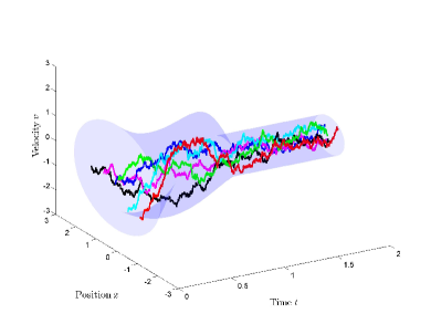
Figure 1: Inertial particles: trajectories in phase space

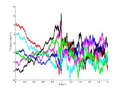
Figure 2: Inertial particles: control effort $u(t)$

Appendix A Relative entropy for stochastic oscillators measures

Consider the same set up as in Section V and let ${\mathcal{D}}$ denote the space of probability measures on path spaces for phase space processes. Consider the process with Ito’s differential

$$dx(t) = v(t)\,dt+n^{-1/2}dZ(t),\quad x(t_{0})=x_{0}\;{\rm a.s.}$$

$$dv(t) = -\beta v(t)\,dt-\frac{1}{m}\nabla V(x(t))dt+u(t)+\sigma dW(t),\quad v(t_{0})=v_{0}\;{\rm a.s.},$$

and let $P_{u}^{n}\in{\mathcal{D}}$ be the measure corresponding to a choice of a specific control law $u\in\mathcal{U}$. Here $Z$ is standard $n$-dimensional Wiener processes independent of $W$ and of the initial conditions $x_{0}$, $v_{0}$. The difference with respect to the model in (33) is that now we have also a “weak” noise $n^{-1/2}dZ(t)$ affecting the configurational variables. Let

$$\Theta^{2}=\mathop{\mathrm{diag}}\left(\frac{1}{n},\sigma^{2}\right)$$

denote the diffusion coefficient matrix for the above model. Next, using Girsanov’s theorem IW ; KS , we compute the Radon-Nikodym derivative $\frac{dP_{u}^{n}}{dP_{0}^{n}}$ between the probability laws for the controlled and the uncontrolled (i.e., with $u=0$) processes.

Let $W_{0}$ be a Wiener measure starting with distribution $\rho_{0}(x,v)dxdv$ of $(x_{0},v_{0})$ at $t=t_{0}$. Since $W_{0}$, $P_{u}^{n}$ and $P_{0}^{n}$ have the same initial marginal, we get

$$\frac{dP_{u}^{n}}{dW_{0}}=\exp\left[\int_{t_{0}}^{t_{1}}\Theta^{-1}\beta_{t}^{P_{u}^{n}}\cdot\Theta^{-1}dX_{t}-\int_{t_{0}}^{t_{1}}\frac{1}{2}\beta_{t}^{P_{u}^{n}}\cdot\Theta^{-2}\beta_{t}^{P_{u}^{n}}dt\right],\quad P_{u}^{n}\;{\rm a.s.},$$

$$\frac{dW_{0}}{dP_{0}^{n}}=\exp\left[-\int_{t_{0}}^{t_{1}}\beta_{t}^{P_{0}^{n}}\cdot\Theta^{-1}dX_{t}+\int_{t_{0}}^{t_{1}}\frac{1}{2}\beta_{t}^{P_{0}^{n}}\Theta^{-2}\beta_{t}^{P_{0}^{n}}dt\right],\quad P_{0}^{n}\;{\rm a.s.}\Rightarrow P_{u}^{n}\;{\rm a.s.}.$$

Therefore,

$$\frac{dP_{u}^{n}}{dP_{0}^{n}} = \exp\left\{\int_{t_{0}}^{t_{1}}\left(\Theta^{-1}\beta_{t}^{P_{u}^{n}}-\Theta^{-1}\beta_{t}^{P_{0}^{n}}\right)\cdot\Theta^{-1}\left(\begin{matrix}dx_{t}\\ dv_{t}\end{matrix}\right)+\frac{1}{2}\int_{t_{0}}^{t_{1}}\left[\beta_{t}^{P_{0}^{n}}\cdot\Theta^{-2}\beta_{t}^{P_{0}^{n}}-\beta_{t}^{P_{u}^{n}}\cdot\Theta^{-2}\beta_{t}^{P_{u}^{n}}\right]dt\right\}$$

$$= \exp\left\{\int_{t_{0}}^{t_{1}}\left(\Theta^{-1}\beta_{t}^{P_{u}^{n}}-\Theta^{-1}\beta_{t}^{P_{0}^{n}}\right)\cdot\left(\begin{matrix}dZ_{t}\\ dW_{t}\end{matrix}\right)+\frac{1}{2}\int_{t_{0}}^{t_{1}}\left(\beta_{t}^{P_{u}^{n}}-\beta_{t}^{P_{0}^{n}}\right)\cdot\Theta^{-2}\left(\beta_{t}^{P_{u}^{n}}-\beta_{t}^{P_{0}^{n}}\right)dt\right\}$$

$$= \exp\left\{\int_{t_{0}}^{t_{1}}\left[\Theta^{-1}\left(\begin{matrix}0\\ u\end{matrix}\right)\right]\cdot\left(\begin{matrix}dZ_{t}\\ dW_{t}\end{matrix}\right)+\frac{1}{2}\int_{t_{0}}^{t_{1}}\left(\begin{matrix}0\\ u\end{matrix}\right)\cdot\Theta^{-2}\left(\begin{matrix}0\\ u\end{matrix}\right)dt\right\}$$

$$= \exp\left\{\int_{t_{0}}^{t_{1}}\frac{1}{\sigma}u\cdot dW_{t}+\int_{t_{0}}^{t_{1}}\frac{1}{2\sigma^{2}}u\cdot udt.\right\}.$$

We observe that this Radon-Nikodym derivative does not depend on $n$.

Now, let $P_{u}$ and $P_{0}$ be the measures in ${\mathcal{D}}$ corresponding to the situation when there is no noise in the position equation (i.e., $n=\infty$). In this case, as expected,

$$\frac{dP_{u}}{dP_{0}}=\int_{t_{0}}^{t_{1}}\frac{1}{\sigma}u\cdot dW_{t}+\int_{t_{0}}^{t_{1}}\frac{1}{2\sigma^{2}}u\cdot udt.$$

To derive this formula, one could have also resorted to a general form of Girsanov’s theorem (IW, , Thm 4.1), (Fischer, , (5.3)). Assuming that the control satisfies the finite energy condition

$${\mathbb{E}}\left[\int_{t_{0}}^{t_{1}}u\cdot udt\right]<\infty,$$

the stochastic integral

$$\int_{t_{0}}^{t_{1}}\frac{1}{\sigma}u\cdot dW_{t}$$

has zero expectation. We then obtain that the relative entropy between $P_{u}$ and $P_{0}$ is

$${\mathbb{D}}(P_{u}\|P_{0})={\mathbb{E}}_{P_{u}}\left[\log\frac{dP_{u}}{dP_{0}}\right]={\mathbb{E}}_{P_{u}}\left[\int_{t_{0}}^{t_{1}}\frac{1}{2\sigma^{2}}u\cdot udt\right],$$ (47)

which is precisely the index in Problem 1 in the case $\Sigma=\sigma I_{n}$.

REFERENCES

- (1) D. Bakry and M. Emery, Diffusions hypercontractives, Séminaire de probabilités XIX, Univ. Strasbourg, Springer, 1985, 177-206..
- (2) F. Baudoin, Bakry-Emery meet Villani, http://arxiv.org/abs/1308.4938v1, Aug. 2013.
- (3) D. Bell, The Malliavin Calculus and Hypoelliptic Differential Operators, Infinite Dimensional Analysis, Quantum Probability and Related Topics, 18, no. 1, 1550001 (2015), 24 pp.
- (4) A. Beurling, An automorphism of product measures, Annals of Mathematics, 1960, 189-200.
- (5) A. Blaquière, Controllability of a Fokker-Planck equation, the Schrödinger system, and a related stochastic optimal control, Dynamics and Control, vol. 2, no. 3, pp. 235-253, 1992.
- (6) M. Bonaldi, L. Conti, P. De Gregorio et al, Nonequilibrium steady-state fluctuations in actively cooled resonators, Phys. Rev. Lett., 103 (2009) 010601.
- (7) Y. Braiman, J. Barhen, and V. Protopopescu, Control of Friction at the Nanoscale, Phys. Rev. Lett. 90, (2003), 094301.
- (8) C. I. Byrnes and C. F. Martin, An integral-invariance principle for nonlinear systems, IEEE Trans. Aut. Contr., 40, pp.983–994, 1995.
- (9) Y. Chen and T.T. Georgiou, Stochastic bridges of linear systems, preprint, http://arxiv.org/abs/1407.3421, IEEE Trans. Aut. Control, to appear, February 2016.
- (10) Y. Chen, T.T. Georgiou and M. Pavon, Optimal steering of a linear stochastic system to a final probability distribution, , Part I, Aug. 2014, http://arxiv.org/abs/1408.2222, IEEE Trans. Aut. Control, to appear, May 2016.
- (11) Y. Chen, T.T. Georgiou and M. Pavon, Optimal steering of a linear stochastic system to a final probability distribution, part II, Oct. 2014, http://arxiv.org/abs/1410.3447, IEEE Trans. Aut. Control, to appear, May 2016.
- (12) Y. Chen, T. Georgiou and M. Pavon, Optimal steering of inertial particles diffusing anisotropically with losses, Oct. 2014, http://arxiv.org/abs/1410.1605, to appear in the Proceedings of the American Control Conference, 2015.
- (13) Y. Chen, T.T. Georgiou and M. Pavon, Entropic and displacement interpolation: a computational approach using the Hilbert metric, June 2015, http://arxiv.org/abs/1506.04255v1, submitted for publication.
- (14) P. Dai Pra, A stochastic control approach to reciprocal diffusion processes, Applied Mathematics and Optimization, 23 (1), 1991, 313-329.
- (15) P.Dai Pra and M.Pavon, On the Markov processes of Schroedinger, the Feynman-Kac formula and stochastic control, in Realization and Modeling in System Theory - Proc. 1989 MTNS Conf., M.A.Kaashoek, J.H. van Schuppen, A.C.M. Ran Eds., Birkaeuser, Boston, 1990, pages 497- 504.
- (16) G. Da Prato, An Introduction to Infinite-Dimensional Analysis, Springer, 2006.
- (17) A. Dembo and O. Zeitouni, Large deviations techniques and applications, Jones and Bartlett Publishers, Boston, 1993.
- (18) M. Doi and S. F. Edwards, The Theory of Polymer Dynamics, Oxford University Press, New York, 1988.
- (19) R. S. Ellis, Entropy, Large deviations and statistical mechanics, Springer-Verlag, New York, 1985.
- (20) P. Faurre, M. Clerget, and F. Germain: Operateurs rationnels positifs, Dunod, Paris, 1979.
- (21) I. Favero and K. Karrai, Nat. Photon. 3, 201 (2009).
- (22) R. Filliger and M.-O. Hongler, Relative entropy and efficiency measure for diffusion-mediated transport processes, J. Physics A: Mathematical and General 38 (2005), 1247-1255.
- (23) R. Filliger, M.-O. Hongler and L. Streit, Connection between an exactly solvable stochastic optimal control problem and a nonlinear reaction-diffusion equation, J. Optimiz. Theory Appl. 137 (2008), 497-505.
- (24) M. Fischer, On the form of the large deviation rate function for the empirical measures of weakly interacting systems, Bernoulli, 20 (4), (2014), 1765-1801.
- (25) W.H. Fleming, Logarithmic transformation and stochastic control, in: W. Fleming and L. Gorostiza, eds., Advances in Filtering and Optimal Stochastic Control, Lecture Notes in Control and Inform. Sciences, Vol. 42, Springer, Berlin, 1982, 131-141.
- (26) W.H. Fleming and R.W. Rishel, Deterministic and Stochastic Optimal Control, Springer-Verlag, Berlin, 1975.
- (27) H. Föllmer, in: Stochastic Processes - Mathematics and Physics , Lect. Notes in Math. 1158 (Springer-Verlag, New York,1986), p. 119.
- (28) H. Föllmer, Random fields and diffusion processes, in: Ècole d’Ètè de Probabilitès de Saint-Flour XV-XVII, edited by P. L. Hennequin, Lecture Notes in Mathematics, Springer-Verlag, New York, 1988, vol.1362,102-203.
- (29) R. Fortet, Résolution d’un système d’equations de M. Schrödinger, J. Math. Pure Appl. IX (1940), 83-105.
- (30) T. T. Georgiou and M. Pavon, Positive contraction mappings for classical and quantum Schroedinger systems, 2014, http://arxiv.org/abs/1405.6650v2, Journal of Mathematical Physics, 56 033301 (2015); doi: 10.1063/1.4915289
- (31) R. Graham, Path integral methods in nonequilibrium thermodynamics and statistics, in Stochastic Processes in Nonequilibrium Systems, L. Garrido, P. Seglar and P.J.Shepherd Eds., Lecture Notes in Physics 84, Springer-Verlag, New York, 1978, 82-138.
- (32) F. Guerra. Processi Dissipativi, Notes for a graduate course on Statistical Mechanics, University of Rome (La Sapienza), 1987 (in Italian).
- (33) U.G.Haussmann and E.Pardoux, Time reversal of diffusions, The Annals of Probability 14, 1986, 1188.
- (34) D.B.Hernandez and M. Pavon, Equilibrium description of a particle system in a heat bath, Acta Applicandae Mathematicae 14 (1989), 239-256.
- (35) L. Hörmander, Hypoelliptic second order differential equations, Acta. Math., 119, 3?4 (1967), 147-171.
- (36) N. Ikeda and S. Watanabe, Stochastic Differential Equations and Diffusion Processes, North-Holland, 1981.
- (37) B. Jamison, The Markov processes of Schrödinger, Z. Wahrscheinlichkeitstheorie verw. Gebiete 32 (1975), 323-331.
- (38) B. Jamison, Reciprocal processes, Probability Theory and Related Fields 30.1 (1974), 65-86.
- (39) R. Kalman, P. Falb and M. Arbib, Topics in Mathematical System Theory, McGraw-Hill, New York, 1969.
- (40) I. Karatzas and S. E. Shreve, Brownian Motion and Stochastic Calculus (Springer-Verlag, New York, 1988).
- (41) K. H. Kim and H. Qian, “Entropy production of Brownian macromolecules with inertia”, Phys. Rev. Lett., 93 (2004), 120602.
- (42) S. Kullback. Information Theory and Statistics, Wiley, 1959.
- (43) Sur la théorie du mouvement brownien, C. R. Acad. Sci. (Paris) 146, 530 533 (1908).
- (44) L. Le Cam, Ann. Stat. 1 (1973), p.38.
- (45) M. Ledoux, Logarithmic Sobolev inequalities for unbounded spin systems revisited, Séminaire de Probabilités XXXV, Springer-Verlag Lecture Notes in Math. 1755, 167-194 (2001).
- (46) H. S. Leff and A. F. Rex (eds.) Maxwell’s Demon 2, Institute of Physics, Bristol, 2003.
- (47) S. Liang, D. Medich, D. M. Czajkowsky, S. Sheng, J. Yuan, and Z. Shao, Ultramicroscopy, 84 (2000), p.119.
- (48) Luo, Y. and Epstein, I. R. (1990) Feedback Analysis of Mechanisms for Chemical Oscillators, in Advances in Chemical Physics, Volume 79 (eds I. Prigogine and S. A. Rice), John Wiley & Sons, Inc., Hoboken, NJ, USA. doi: 10.1002/9780470141281.ch3
- (49) F. Marquardt and S. M. Girvin, Optomechanics, Physics 2, 40 (2009).
- (50) J. M. W. Milatz, J. J. Van Zolingen, and B. B. Van Iperen, Physica (Amsterdam)19, 195 (1953).
- (51) P. C. Müller, Asymptotische Stabilität von linearen mechaniscen Systemen mit positiv semidefiniter Dämpfungsmatrix, Z. Angew. Math. Mech., 51 (1971),T197-T198.
- (52) E. Nelson, Dynamical Theories of Brownian Motion, Princeton University Press, Princeton, 1967.
- (53) E. Nelson, Stochastic mechanics and random fields, in Ècole d’Ètè de Probabilitès de Saint-Flour XV-XVII, edited by P. L. Hennequin, Lecture Notes in Mathematics, Springer-Verlag, New York, 1988, vol.1362, pp. 428-450.
- (54) M.Pavon, Critical Ornstein-Uhlenbeck processes, Appl. Math. and Optimiz. 14 (1986), 265-276.
- (55) M.Pavon and A.Wakolbinger, On free energy, stochastic control, and Schroedinger processes, Modeling, Estimation and Control of Systems with Uncertainty, G.B. Di Masi, A.Gombani, A.Kurzhanski Eds., Birkauser, Boston, 1991, 334-348.
- (56) M. Pavon and F. Ticozzi, On entropy production for controlled Markovian evolution, J. Math. Phys., 47, 06330, doi:10.1063/1.2207716 (2006).
- (57) M. Pavon and F. Ticozzi, Discrete-time classical and quantum Markovian evolutions: Maximum entropy problems on path space, J. Math. Phys., 51, 042104-042125 (2010) doi:10.1063/1.3372725.
- (58) M. Poot and H. S. J. van der Zant, Mechanical systems in the quantum regime, Physics Reports, 511 (5) (2012), 273-335.
- (59) H. Qian, “Relative entropy: free energy associated with equilibrium fluctuations and nonequilibrium deviations”, Physical Review E, 63 (2001), p. 042103.
- (60) P. Reimann, Brownian motors: noisy transport far from equilibrium, Phys. Rep. 361, (2002) 57.
- (61) L.M. Ricciardi and L. Sacerdote, The Ornstein-Uhlenbeck process as a model for neuronal activity Biological Cybernetics (1979) Volume 35(1), pp 1-9.
- (62) E. Schrödinger, Über die Umkehrung der Naturgesetze, Sitzungsberichte der Preuss Akad. Wissen. Berlin, Phys. Math. Klasse (1931), 144-153.
- (63) E. Schrödinger, Sur la théorie relativiste de l’electron et l’interpretation de la mécanique quantique, Ann. Inst. H. Poincaré 2, 269 (1932).
- (64) K. C. Schwab and M. L. Roukes, Phys. Today 58, No. 7, 36 (2005).
- (65) D. Stroock, Probability Theory, an Analytic View, Cambridge University Press, 1993.
- (66) J. Tamayo, A. D. L. Humphris, R. J. Owen, and M. J. Miles, Biophys., 81 (2001), p. 526.
- (67) H. N. Tan and J. L. Wyatt, Thermodynamics of electrical noise in a class of nonlinear RLC networks, IEEE Tran. Circuits and Systems 32 (1985), 540-558.
- (68) C. Villani, Topics in optimal transportation, AMS, 2003, vol. 58.
- (69) C. Villani, Hypocoercivity, Mem. Amer. Math. Soc. 202 (2009), n. 950.
- (70) A. Vinante, M. Bignotto, M. Bonaldi et al., Feedback Cooling of the Normal Modes of a Massive Electromechanical System to Submillikelvin Temperature, Physical Review Letters 101 (2008), 033601.
- (71) A. Wakolbinger, Schroedinger bridges from 1931 to 1991, in Proc. of the 4th Latin American Congress in Probability and Mathematical Statistics, Mexico City 1990, Contribuciones en probabilidad y estadistica matematica, 3 (1992), 61-79.
- (72) H. Wimmer, Inertia theorems for matrices, controllability, and linear vibrations, Linear Algebra and its Applications, 8 (1974), 337-343.