Hybrid-order Poincaré sphere

Abstract

In this work, we develop a hybrid-order Poincaré sphere to describe the evolution of polarization states of wave propagation in inhomogeneous anisotropic media. We extend the orbital Poincaré sphere and high-order Poincaré sphere to a more general form. Polarization evolution in inhomogeneous anisotropic media with special geometry can be conveniently described by state evolution along the longitude line on the hybrid-order Poincaré sphere. Similar to that in previously proposed Poincaré spheres, the Berry curvature can be regarded as an effective magnetic field with monopole centered at the origin of sphere and Berry connection can be interpreted as the vector potential. Both the Berry curvature and the Pancharatnam-Berry phase on the hybrid-order Poincaré sphere are demonstrated to be proportional to the variation of total angular momentum. Our scheme provides a convenient method to describe the spin-orbit interaction in inhomogeneous anisotropic media.

Polarization and phase are two intrinsic features of electromagnetic waves Born1997 . Fundamental polarization states, such as linear, circular, and elliptical polarizations, have a spatial homogeneous distribution. In 1892, a prominent geometric representation of polarization known as the Poincaré sphere is proposed to describe the polarization state of light as a point on the surface of a unit sphere Poincare1892 . The Poincaré sphere unifies the fundamental polarizations, where the polarization states represented by a complex Jones vectors are mapped to the sphere’s surface through the Stokes parameters in the sphere’s Cartesian coordinates. This geometric characterization not only greatly simplifies the calculations of geometric phase, but also provides a deeper insight into physical mechanisms. As a result, the representation of Poincaré sphere has become an important technique to deal with the polarization evolution in different physical systems.

Recently, the orbital Poincaré sphere has been proposed as a geometrical construction to represent the state evolution in phase space Padgett1999 . In analogy to the space of polarization, the north and south poles of the orbital Poincaré sphere correspond to the Laguerre-Gaussian modes with opposite topological charges. The points in the equator of the sphere correspond to Hermite-Gaussian modes Galvez2003 ; Karimi2010 . In past several years, high-order solutions with a spatial inhomogeneous polarization and phase have drawn much attention Zhan2009 . More recently, the high-order Poincaré sphere has been proposed to describe the evolution of both polarization and phase Milione2011 ; Holleczek2011 . The north and south poles of the high-order Poincaré sphere represent the opposite spin states and orbital states. Any state on the high-order Poincaré sphere, can be realized by a superposition of the two orthogonal states Milione2012 ; Cardano2012 ; Chen2014 . However, the high-order solutions on high-order Poincaré sphere are still confined to some special cases. Hence, it is necessary for us to extend the orbital Poincaré sphere and high-order Poincaré sphere to a more general form.

In this work, we develop a hybrid-order Poincaré sphere to describe the evolution of phase and polarization of wave propagating in inhomogeneous anisotropic media. We find that the representation of the polarization states in inhomogeneous anisotropic media has a similar expression of polarization states on high-order Poincaré sphere Milione2011 ; Holleczek2011 with only the orbital states being different. This interesting property motivates us to develop a hybrid-order Poincaré sphere to describe the evolution of polarization states, and therefore extending the high-order Poincaré sphere and orbital Poincaré sphere to a more general form. It is known that the orbital states in the two poles of orbital and high-order Poincaré spheres have the same value but opposite signs. Unlike the previously reported cases, the orbital states on hybrid-order Poincaré sphere should not be confined to this certain condition and can be chosen arbitrarily. We show that the polarization evolution in inhomogeneous anisotropic media with special geometry can be conveniently described by state evolution along the longitude line on the hybrid-order Poincaré sphere. Furthermore, Berry connection, Berry curvature, and Pancharatnam-Berry phase associated with the evolution of polarization state are discussed.

I Hybrid-order Poincaré sphere

We now develop a hybrid-order Poincaré sphere to describe the evolution of polarization and phase in inhomogeneous anisotropic media. It is assumed that the media are composed of local waveplates whose optical axis directions are specified by a space-variant angle

$$\alpha(r,\varphi)=q\varphi+\alpha_{0},$$ (1)

where $r$ is the radial coordinate, $\varphi$ is the azimuthal coordinate, $\alpha_{0}$ is a constant angle specifying the initial orientation on the axis $x$, and $q$ is a constant specifying the topological charge. The inhomogeneous birefringent elements having specified geometry can be designated as $q$-plates Marrucci2006 .

Let us consider that the $q$-plate is illuminated by a circularly polarized vortex wave $|\mathbf{\psi}\rangle={\sqrt{2}}/2(\mathbf{\hat{e}}_{x}+i\sigma\mathbf{\hat{e}}_{y})\exp(il\varphi)$ with spin angular momentum (SAM) $\sigma\hbar$ Beth1936 and orbit angular momentum (OAM) $l\hbar$ Allen1992 , where $\sigma=+1$ for the left-handed circular (LHC) polarization and $\sigma=-1$ for the right-handed circular (RHC) one. The evolution of optical field in the inhomogeneous medium can be obtained in Appendix A as

$$|\mathbf{\psi}_{l,m}\rangle = \cos\frac{\delta}{2}\frac{\sqrt{2}}{2}(\mathbf{\hat{e}}_{x}+i\sigma\mathbf{\hat{e}}_{y})\exp(il\varphi)$$ (2)

$$+\sin\frac{\delta}{2}\frac{\sqrt{2}}{2}(\mathbf{\hat{e}}_{x}-i\sigma\mathbf{\hat{e}}_{y})\exp(im\varphi)$$

$$\times\exp[i(2\sigma\alpha_{0}-\frac{\pi}{2})].$$

Here, $m=l+2\sigma{q}$. It should be noted that diffraction inside the $q$-plate is neglected, so that only evolution of polarization and phase is taking place. This is valid as long as the thickness of the medium is small as compared with a Rayleigh diffraction length. The field in the $q$-plate can be regarded as a superposition of a first wave that has the same SAM and OAM as the input one, and a second wave having reversed SAM and a modified OAM given by $m\hbar$. It means that the input wave only partially occurs spin-to-orbital angular momentum conversion Marrucci2008 . The field amplitudes of the two components of the field depend on the birefringent retardation $\delta$, and are given by $\cos\delta/2$ and $\sin\delta/2$, respectively. In addition, a singularity should be generated around central region of $q$-plate.

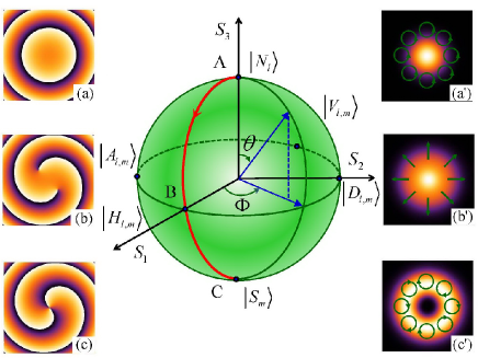
Figure 1: (Color online) Schematic illustration of the evolution of phase and polarization on hybrid-order Poincaré sphere. Insets (a)-(c) show the the phase for points A, B, and C, respectively. Insets (a^′)-(c^′) show the polarization state of the three points. Here, we assume the north pole with state $\sigma=+1$ and $l=0$, while the south pole with $\sigma=-1$ and $m=+2$.

We note that the field represented by Eq. (2) has a similar expression to the field represented by high-order Poincaré sphere Milione2011 ; Holleczek2011 with only the orbital states being different. It inspires us to develop a hybrid-order Poincaré sphere to describe the evolution of phase and polarization. The field for a monochromatic paraxial light beam can be expressed as a two dimensional Jones vector:

$$|\mathbf{\psi}_{l,m}\rangle=\mathbf{\psi}_{N}^{l}|\mathbf{N}_{l}\rangle+\mathbf{\psi}_{S}^{m}|\mathbf{S}_{m}\rangle,$$ (3)

where

$$|\mathbf{N}_{l}\rangle=\frac{\sqrt{2}}{2}(\mathbf{\hat{e}}_{x}+i\sigma\mathbf{\hat{e}}_{y})\exp(il\varphi),$$ (4)

$$|\mathbf{S}_{m}\rangle=\frac{\sqrt{2}}{2}(\mathbf{\hat{e}}_{x}-i\sigma\mathbf{\hat{e}}_{y})\exp(im\varphi).$$ (5)

Here, $|\mathbf{N}_{l}\rangle$ and $|\mathbf{S}_{m}\rangle$ with different topological charges construct an orthogonal polarization basis. Any polarization state on hybrid-order Poincaré can be described as a superposition of the orthogonal bases with coefficients $\mathbf{\psi}_{N}^{l}$ and $\mathbf{\psi}_{S}^{m}$, respectively.

We now map the polarization states on hybrid-order Poincaré sphere by representing the Stokes parameters in the sphere’s Cartesian coordinates. According to Eqs. (4) and (5), we redefine the Stokes parameters as Born1997

$$S_{0}^{l,m}=|\mathbf{\psi}_{N}^{l}|^{2}+|\mathbf{\psi}_{S}^{m}|^{2},$$ (6)

$$S_{1}^{l,m}=2|\mathbf{\psi}_{N}^{l}||\mathbf{\psi}_{S}^{m}|\cos\Phi,$$ (7)

$$S_{2}^{l,m}=2|\mathbf{\psi}_{N}^{l}||\mathbf{\psi}_{S}^{m}|\sin\Phi,$$ (8)

$$S_{3}^{l,m}=|\mathbf{\psi}_{N}^{l}|^{2}-|\mathbf{\psi}_{S}^{m}|^{2},$$ (9)

where $\Phi=\arg(\mathbf{\psi}_{N}^{l})-\arg(\mathbf{\psi}_{S}^{m})$, $|\mathbf{\psi}_{N}^{l}|^{2}$ and $|\mathbf{\psi}_{S}^{m}|^{2}$ are the intensities of $|\mathbf{N}_{l}\rangle$ and $|\mathbf{S}_{m}\rangle$, respectively. Using $S_{1}^{l,m}$, $S_{2}^{l,m}$, and $S_{3}^{l,m}$ as the sphere’s Cartesian coordinates, we construct a new Poincaré sphere with $S_{0}^{l,m}$ the unit radius. Equations (4) and (5) denote the states on two poles with orthogonal circular polarizations. It is worth noting that $|\mathbf{N}_{l}\rangle$ and $|\mathbf{S}_{m}\rangle$ generally have different topological charges, i.e., $l\neq m$. Therefore, we term the new Poincaré sphere as hybrid-order Poincaré sphere.

Generally, the equatorial points on the hybrid-order Poincaré sphere represent a superposition of equal intensities of the two orthogonal states. The horizontal and vertical polarization basis ($|\mathbf{H}_{l,m}\rangle$, $|\mathbf{V}_{l,m}\rangle$) can be obtained through the relations $|\mathbf{H}_{l,m}\rangle=(|\mathbf{N}_{l}\rangle+|\mathbf{S}_{m}\rangle)/2$ and $|\mathbf{V}_{l,m}\rangle=-i(|\mathbf{N}_{l}\rangle-|\mathbf{S}_{m}\rangle)/2$, then we have

$$|\mathbf{H}_{l,m}\rangle = \exp\frac{i(l+m)\varphi}{2}\bigg{[}\cos\frac{(l-m)\varphi}{2}\mathbf{\hat{e}}_{x}$$ (10)

$$+\sin\frac{(l-m)\varphi}{2}\mathbf{\hat{e}}_{y}\bigg{]},$$

$$|\mathbf{V}_{l,m}\rangle = \exp\frac{i(l+m)\varphi}{2}\bigg{[}\cos\left(\frac{l-m}{2}\varphi+\frac{\pi}{2}\right)\mathbf{\hat{\hat{e}}}_{x}$$ (11)

$$+\sin\left(\frac{l-m}{2}\varphi+\frac{\pi}{2}\right)\mathbf{\hat{\hat{e}}}_{y}\bigg{]},$$

with coefficients $\mathbf{\psi}_{H}^{l,m}=(\mathbf{\psi}_{N}^{l}+\mathbf{\psi}_{S}^{m})/\sqrt{2}$ and $\mathbf{\psi}_{V}^{l,m}=i(\mathbf{\psi}_{N}^{l}-\mathbf{\psi}_{S}^{m})/\sqrt{2}$. Similarly, the diagonal and antidiagonal polarization basis $|\mathbf{D}_{l,m}\rangle$ and $|\mathbf{A}_{l,m}\rangle$ can be obtained through the relations $|\mathbf{D}_{l,m}\rangle=(|\mathbf{H}_{l,m}\rangle+|\mathbf{V}_{l,m}\rangle)/\sqrt{2}$ and $|\mathbf{A}_{l,m}\rangle=(|\mathbf{H}_{l,m}\rangle-|\mathbf{V}_{l,m}\rangle)/\sqrt{2}$, respectively, and we have

$$|\mathbf{D}_{l,m}\rangle = \exp\frac{i(l+m)\varphi}{2}\bigg{[}\cos\left(\frac{l-m}{2}\varphi+\frac{\pi}{4}\right)\mathbf{\hat{e}}_{x}$$ (12)

$$+\sin\left(\frac{l-m}{2}\varphi+\frac{\pi}{4}\right)\mathbf{\hat{e}}_{y}\bigg{]},$$

$$|\mathbf{A}_{l,m}\rangle = \exp\frac{i(l+m)\varphi}{2}\bigg{[}\cos\left(\frac{l-m}{2}\varphi+\frac{3\pi}{4}\right)\mathbf{\hat{e}}_{x}$$ (13)

$$+\sin\left(\frac{l-m}{2}\varphi+\frac{3\pi}{4}\right)\mathbf{\hat{e}}_{y}\bigg{]},$$

with coefficients $\mathbf{\psi}_{D}^{l,m}=(\mathbf{\psi}_{H}^{l,m}+\mathbf{\psi}_{V}^{l,m})/\sqrt{2}$ and $\mathbf{\psi}_{A}^{l,m}=(\mathbf{\psi}_{H}^{l,m}-\mathbf{\psi}_{V}^{l,m})/\sqrt{2}$. Note that the equatorial points represent vector vortex waves and the relative phase of the superposition determines the orientation of the longitude on equator.

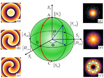
Figure 2: (Color online) Schematic illustration of the evolution of phase and polarization on hybrid-order Poincaré sphere. Insets (a)-(c) show the evolution the phase for points $A$, $B$, and $C$, respectively. Insets (a^′)-(c^′) show the evolution of polarization of the three points. Here, we assume the noth pole with state $\sigma=+1$ and $l=0$, while the south pole with $\sigma=-1$ and $m=-2$.

Figures 1 and 2 show the two cases for the evolution of phase and polarization on hybrid-order Poincaré spheres. Comparing with the high-order Poincaré sphere, the hybrid-order Poincaré sphere has two special features: (1) The orbital states on hybrid-order Poincaré sphere should not be confined to have the same value and opposite signs. As a result, the cylindrical vector vortex beam can be represented by the equatorial points. Intermediate points between the poles and equator represent elliptically polarized vector vortex beam. (2) Polarization and phase evolution in any $q$-plate can be conveniently described by state evolution along the longitude line on the hybrid-order Poincaré sphere. These features will be described in detail in the next section.

II Berry connection, Berry curvature, and geometric phase

From a basic geometric transformation on the Poincaré sphere, the factor of $\varphi\rightarrow\Phi/2$ is a consequence of transformation between the physical SU(2) space of the light beam and the topological SO(3) space of the hybrid-order Poincaré sphere Milione2012 . For a monochromatic wave, the polarization states can be represented as a two dimensional Jones vector given by

$$|\mathbf{\psi(\theta,\Phi)}\rangle=\cos\frac{\theta}{2}|\mathbf{N}_{l}\rangle+\sin\frac{\theta}{2}|\mathbf{S}_{m}\rangle\exp(+i\sigma\Phi).$$ (14)

where

$$|\mathbf{N}_{l}\rangle=\frac{\sqrt{2}}{2}(\mathbf{\hat{e}}_{x}+i\sigma\mathbf{\hat{e}}_{y})\exp(il\Phi/2),$$ (15)

$$|\mathbf{S}_{m}\rangle=\frac{\sqrt{2}}{2}(\mathbf{\hat{e}}_{x}-i\sigma\mathbf{\hat{e}}_{y})\exp(im\Phi/2).$$ (16)

Here, $(\theta,\Phi)$ are the latitude and longitude on the sphere. We have introduced the relation $\theta=\delta$ and $\Phi=2\alpha_{0}\pm\pi/2$, where the choice of signs depends on the circular polarization handedness of the input wave. Equations (15) and (16) represent orthogonal circular polarizations with different topological charges $l$ and $m$.

Similar to the previously proposed Poincaré spheres, the Berry connection can be written as Berry1984

$$\mathbf{A}=i\langle\psi(\mathbf{R})|\nabla_{R}|\psi(\mathbf{R})\rangle.$$ (17)

The components of Berry connection can be obtained in Appendix B as

$$\mathbf{A}_{\rho}=0,$$ (18)

$$\mathbf{A}_{\theta}=0,$$ (19)

$$\mathbf{A}_{\Phi}=-\frac{1}{4\rho\sin\theta}[l(1+\cos\theta)+(m+2\sigma)(1-\cos\theta)].$$ (20)

The Berry curvature for the hybrid-order Poincaré sphere plays the role of “magnetic field” in the parameter space and is given by

$$\mathbf{V(R)}=-\nabla_{\mathbf{R}}\times\mathbf{A}.$$ (21)

Substituting Eqs. (18)-(20) into Eq. (21) we get

$$\mathbf{V(R)}=\frac{l-(m+2\sigma)}{4\rho^{2}}\mathbf{\hat{\rho}}.$$ (22)

Equation (22) shows the Berry curvature is proportional to the variation of total angular momentum of light, a sum of SAM and OAM.

In Berry’s framework a state $\psi(\mathbf{R})$ undergoes a cyclic transformation over a circuit $C$ in parameter space $\mathbf{R}$, and then return to the initial state, an additional phase in addition to dynamic phase arises which is given by

$$\gamma(C)=-\int\int_{C}d\mathbf{S}\cdot\mathbf{V(R)},$$ (23)

where $d\mathbf{S}=\rho^{2}\sin{\theta}d{\rho}d{\theta}d{\Phi}\mathbf{\hat{\rho}}$ Berry1987 . Substituting Eq. (22) into Eq. (23), the resulting geometric phase on the hybrid-order Poincaré sphere is then given by

$$\gamma(C)=-\frac{l-(m+2\sigma)}{4}\Omega,$$ (24)

where $\Omega$ is the surface area on the hybrid-order Poincacé sphere enclosed by the circuit $C$. Equation (24) shows that the geometric phase is directly proportional to the variation of total angular momenta of light. Interestingly, when the two modes have the same total angular momentum (as for $q=1$) both the Berry curvature and the geometrical phase vanish, since the photon crossing the $q$-plate does not change its total angular momentum Marrucci2008 .

On the plane-wave Poincaré sphere, the evolution of polarization states in a homogeneous waveplate can be described as the transformations of longitude and latitude. A quarter-wave plate can transform a circular polarization light to a linear polarization one. This transformation on the plane-wave Poincaré sphere can be described as polarization states from the north pole to a point on the equator, and whose longitude depends on the orientation of the optical axis. Rotation of the waveplate through an angle $\alpha$ advances the longitude by an angle $2\alpha$. A half-wave plate can transform a left-handed circular polarization to a right-handed one. This transformation is presented by a move from pole to pole along a great circle. This dependence can be easily demonstrated if we regard the half-wave plate as two identical quarter-wave plates Padgett1999 .

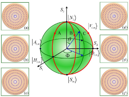
Figure 3: (Color online) Schematic illustration of the evolution of states on the hybrid-order Poincaré sphere. As an example, we choose $q=1$ and $l-m=2$. Insets (a)-(c) realization of the evolution along different longitude lines from the north pole to south pole by half-wave $q$-plate with different initial angles $\alpha_{0}$. Insets (a^′)-(c^′) realization of the evolution along different longitude lines from south pole to north pole. The initial angle of $q$-plate can be obtained by the relation $\Phi=2\alpha_{0}-\pi/2$ from the north pole to south pole, and $\Phi=2\alpha_{0}+\pi/2$ from the south pole to north pole.

On the hybrid-order Poincaré sphere, the evolution of polarization states in an inhomogeneous waveplate can also be described as the transformations of longitude and latitude. A quarter-wave $q$-plate transforms a circular polarization light to a cylindrical vector polarization one. This transformation on the hybrid-order Poincaré sphere can be described as polarization states from the north pole to a point on the equator, and whose longitude depends on the orientation of the initial angle of $q$-plate. Rotation of the initial angle $\alpha_{0}$ of $q$-plate advances the longitude by an angle $2\alpha_{0}$ as shown in Fig. 3. Similarly, a half-wave $q$-plate transforms left-handed circular polarization to right-handed one. This transformation is presented by a move from one pole to the other pole along a great circle. Therefore, our scheme provides a convenient method to describe the spin-orbit interaction. In a word, the phase retardation of $q$-plate determined the latitude of state on the hybrid-order Poincaré sphere, while the longitude is determined by the initial orientation angle $\alpha_{0}$. We therefore can achieve any vector vortex beams by controlling the phase retardation and initial orientation angle of $q$-plate. An important point should be noted that for general cases with $q\neq 1$, $\alpha_{0}$ can be varied by rigidly rotating the $q$-plate, we therefore can achieve a similar effect of selecting the longitude line.

For the case of $\sigma=\pm 1$ and $l=-m$, the hybrid-order Poincaré sphere reduces to the high-order Poincaré sphere Milione2011 ; Holleczek2011 . For the case of $\sigma=0$ and $l=-m$, the hybrid-order Poincaré sphere reduces to the orbital Poincaré sphere Padgett1999 ; Galvez2003 . For the case of $\sigma=\pm 1$ and $l=m=0$ the hybrid-order Poincaré sphere reduces to the well-known fundamental plane-wave Poincaré sphere. In addition, the hybrid-order Poincaré sphere can also be extended to describe the electron vortex beam where the Pancharatnam-Berry phase is related to real magnetic field Karimi2012 . Note that the rotational symmetry of a light beam’s electric field gives rise to the temporal frequency shift or rotational Doppler effect Garetz1979 ; Simon1988 ; Birula1997 ; Courtial1998 . For a spatial rotation of anisotropic axis in plane transverse to the propagation direction of the beam, the rotational Doppler effect is valid by replacing the temporal frequency shift with a spatial one Bliokh2008 ; Niv2008 . The hybrid-order Poincaré may provide a convenient route to describe the spatial Doppler effect.

III Conclusions

In conclusions, we have proposed a hybrid-order Poincaré sphere to describe the evolution of polarization states in inhomogeneous anisotropic media. The metasurface (a two-dimensional electromagnetic nanostructure) Kildishev2013 is expected to be a good candidate for realizing the evolution of polarization states on hybrid Poincaé sphere. By correctly controlling the local orientation and geometrical parameters of the nanograting, one can achieve any desired polarization distribution on hybrid-order Poincaré sphere Liu2014 ; Yi2014 . We have demonstrated that both the Berry curvature and the Pancharatnam-Berry phase on the hybrid-order Poincaré sphere is proportional to the variation of total angular momentum. A representation of beams in the framework of the hybrid-order Poincaré sphere would offer great utility to describe the spin-orbit interaction and Pancharatnam-Berry phase.

Appendix A Calculation of beam evolution in inhomogeneous media

In this appendix we give a detailed calculation of beam evolution in inhomogeneous anisotropic media. The manipulation of polarization state and phase is obtained by using the effective birefringent nature of inhomogeneous media. If the orientation of the optical axis is space-variant at each location, the grating can be described by the space dependent matrix Yariv2007 :

$$\mathbf{T}(r,\varphi)=\mathbf{M}(r,\varphi)\mathbf{J}\mathbf{M}^{-1}(r,\varphi).$$ (25)

Here, $\mathbf{J}$ is the Jones matrix of a uniaxial crystal, and

$$\mathbf{M}(r,\varphi)=\left(\begin{array}[]{cc}\cos\alpha&\sin\alpha\\ \sin\alpha&-\cos\alpha\end{array}\right),$$ (26)

where $\alpha(r,\varphi)$ is the local orientation of the optical axis. It can be easily proved that the Jones matrix $\mathbf{T}(r,\varphi)$ of the optical field interacting with the inhomogeneous anisotropic media at each transverse position $(r,~{}\varphi)$ is given by following:

$$\mathbf{T}(r,\varphi)=\cos\frac{\delta}{2}\left(\begin{array}[]{cc}1&0\\ 0&1\end{array}\right)-i\sin\frac{\delta}{2}\left(\begin{array}[]{cc}\cos 2\alpha&\sin 2\alpha\\ \sin 2\alpha&-\cos 2\alpha\end{array}\right).$$ (27)

The Jones vector of electric field associated with input wave is given by $|\mathbf{\psi}\rangle={\sqrt{2}}/2(\mathbf{\hat{e}}_{x}+i\sigma\mathbf{\hat{e}}_{y})\exp(il\varphi)$. The beam in the inhomogeneous anisotropic media $|\mathbf{\psi(\delta,\varphi)}\rangle=\mathrm{T}(r,\varphi)|\mathbf{\psi}\rangle$ can be written as

$$|\mathbf{\psi(\delta,\varphi)}\rangle = \cos\frac{\delta}{2}\exp(il\varphi)\frac{\sqrt{2}}{2}(\mathbf{\hat{e}}_{x}+i\sigma\mathbf{\hat{e}}_{y})-i\sin\frac{\delta}{2}$$ (28)

$$\times\frac{\sqrt{2}}{2}(\mathbf{\hat{e}}_{x}+i\sigma\mathbf{\hat{e}}_{y})\exp[i(l\varphi+2\sigma\alpha)].$$

Here, we pay our attention to the evolution of polarization and phase, and therefore ignoring the evolution of intensity in the radial coordinate.

Appendix B Calculation of Berry connection and Berry curvature

In this appendix we give a detailed calculation of Berry connection and Berry curvature. From Eq. (17) the three components of Berry connection can be written as

$$\mathbf{A}_{\rho}=i\langle\psi(\mathbf{R})|\partial_{\rho}|\psi(\mathbf{R})\rangle,$$ (29)

$$\mathbf{A}_{\theta}=i\langle\psi(\mathbf{R})|\partial_{\theta}|\psi(\mathbf{R})\rangle/\rho,$$ (30)

$$\mathbf{A}_{\Phi}=i\langle\psi(\mathbf{R})|\partial_{\varphi}|\psi(\mathbf{R})\rangle/(\rho\sin\theta).$$ (31)

As $|\psi(\mathbf{R})\rangle$ is independent of $\rho$, and $\partial_{\rho}|\psi(\mathbf{R})\rangle=0$. Substituting it into Eq. (29) we get

$$\mathbf{A}_{\rho}=i\langle\psi(\mathbf{R})|\partial_{\rho}|\psi(\mathbf{R})\rangle=0.$$ (32)

From Eq. (14), we know that

$$|\partial_{\theta}\mathbf{\psi(\mathbf{R})}\rangle=-\frac{1}{2}\sin\frac{\theta}{2}|\mathbf{N}_{l}\rangle+\frac{1}{2}\cos\frac{\theta}{2}|\mathbf{S}_{m}\rangle\exp(+i\sigma\Phi).$$ (33)

Substituting it into Eq. (30) we get

$$\mathbf{A}_{\theta} = i\langle\psi(\mathbf{R})|\partial_{\theta}|\psi(\mathbf{R})\rangle/\rho$$ (34)

$$= -\frac{1}{4\rho}\sin\theta\langle\mathbf{N}_{l}|\mathbf{N}_{l}\rangle+\frac{1}{4\rho}\sin\theta\langle\mathbf{S}_{m}|\mathbf{S}_{m}\rangle$$

$$= 0.$$

From Eq. (14), we get

$$|\partial_{\Phi}\mathbf{\psi(\mathbf{R})}\rangle=\frac{il}{2}\sin\frac{\theta}{2}|\mathbf{N}_{l}\rangle+\frac{i(m+2\sigma)}{2}\cos\frac{\theta}{2}|\mathbf{S}_{m}\rangle e^{+i\sigma\Phi}.$$ (35)

Substituting it into Eq. (31) we get

$$\mathbf{A}_{\Phi} = i\langle\psi(\mathbf{R})|\partial_{\Phi}|\psi(\mathbf{R})\rangle/(\rho\sin\theta)$$

$$= -\frac{1}{4\rho\sin\theta}[l(1+\cos\theta)+(m+2\sigma)(1-\cos\theta)].$$

The Berry curvature is given by $\mathbf{V(R)}=-\nabla_{\mathbf{R}}\times\mathbf{A}$, where the Laplace operator in the sphere coordinate representations can be written as

$$\nabla=\frac{d}{d\rho}\mathbf{\rho}+\frac{1}{\rho}\frac{d}{d\theta}\mathbf{\theta}+\frac{1}{\rho\sin\theta}\frac{d}{d\Phi}\mathbf{\Phi}.$$ (37)

We then get

$$\mathbf{V(R)}=\left|\begin{array}[]{ccc}\mathbf{\rho}&\rho\mathbf{\theta}&\rho\sin\theta\mathbf{\Phi}\\ \frac{d}{d\rho}&\frac{d}{d\theta}&\frac{d}{d\Phi}\\ \mathbf{A}_{\rho}&\rho\mathbf{A}_{\theta}&\rho\sin\theta\mathbf{A}_{\Phi}\end{array}\right|.$$ (38)

Because of $\mathbf{A_{\rho}}=\mathbf{A_{\theta}}=0$, we can just obtain a component from Eq. (38) as

$$\mathbf{V_{\rho}}=\frac{\frac{d}{d\rho}(\rho\sin\theta\mathbf{A}_{\Phi})}{\rho^{2}\sin\theta}.$$ (39)

After substituting Eq. (LABEL:APhiII) into Eq. (39), we get

$$\mathbf{V_{\rho}(R)}=\frac{l-(m+2\sigma)}{4\rho^{2}},$$ (40)

which is proportional to the variation of total angular momenta of light.

References

- (1) M. Born and E. Wolf, Principles of Optics (University Press, Cambridge, 1997).
- (2) H. Poincaré, Theorie Mathematique de la Lumiere (Gauthiers-Villars, Paris, 1892).
- (3) M. J. Padgett and J. Courtial, Opt. Lett. 24, 430 (1999).
- (4) E. J. Galvez, P. R. Crawford, H. I. Sztul, M. J. Pysher, P. J. Haglin, and R. E. Williams, Phys. Rev. Lett. 90, 203901 (2003).
- (5) E. Karimi, S. Slussarenko, B. Piccirillo, L. Marrucci, and E. Santamato, Phys. Rev. A 81, 053813 (2010).
- (6) Q. Zhan, Adv. Opt. Photon. 1, 1 (2009).
- (7) G. Milione, H. I. Sztul, D. A. Nolan, and R. R. Alfano, Phys. Rev. Lett. 107, 053601 (2011).
- (8) A. Holleczek, A. Aiello, C. Gabriel, C. Marquardt, G. Leuchs, Opt. Express 19, 9714 (2011).
- (9) G. Milione, S. Evans, D. A. Nolan, and R. R. Alfano, Phys. Rev. Lett. 108, 190401 (2012).
- (10) F. Cardano, E. Karimi, S. Slussarenko, L. Marrucci, C. de Lisio, and E. Santamato, Appl. Opt. 51, C1 (2012).
- (11) S. Chen, X. Zhou, Y. Liu, X. Ling, H. Luo, and S. Wen, Opt. Lett. 39, 5274 (2014).
- (12) L. Marrucci, C. Manzo, and D. Paparo, Phys. Rev. Lett. 96, 163905 (2006).
- (13) R. A. Beth, Phys. Rev. 50, 115 (1936).
- (14) L. Allen, M. W. Beijersbergen, R. J. C. Spreeuw, and J. P. Woerdman, Phys. Rev. A 45, 8185 (1992).
- (15) L. Marrucci, Mol. Cryst. Liq. Cryst. 488, 148 (2008).
- (16) M. V. Berry, Proc. R. Soc. Lond. A 392, 45 (1984).
- (17) M. V. Berry, J. Mod. Opt. 34, 1401 (1987).
- (18) E. Karimi, L. Marrucci, V. Grillo, and E. Santamato, Phys. Rev. Lett. 108, 044801 (2012).
- (19) B. A. Garetz and S. Arnold, Opt. Commun. 31, 1 (1979).
- (20) R. Simon, H. J. Kimble, and E. C. G. Sudarshan, Phys. Rev. Lett. 61, 19 (1988).
- (21) I. Bialynicki-Birula and Z. Bialynicka-Birula, Phys. Rev. Lett. 78, 2539 (1997).
- (22) J. Courtial, K. Dholakia, D. A. Robertson, L. Allen, and M. J. Padgett, Phys. Rev. Lett. 80, 3217 (1998).
- (23) K. Y. Bliokh, Y. Gorodetski, V. Kleiner, and E. Hasman, Phys. Rev. Lett. 101, 030404 (2008).
- (24) A. Niv, Y. Gorodetski, V. Kleiner, and E. Hasman, Opt. Lett. 33, 2910 (2008).
- (25) A. V. Kildishev, A. Boltasseva, and V. M. Shalaev, Science 339, 1232009 (2013).
- (26) Y. Liu, X. Ling, X. Yi, X. Zhou, H. Luo, and S. Wen, Appl. Phys. Lett. 104, 191110 (2014).
- (27) X. Yi, X. Ling, Z. Zhang, Y. Li, X. Zhou, Y. Liu, S. Chen, H. Luo, and S. Wen, Opt. Express 22, 17207 (2014).
- (28) A. Yariv and P. Yeh, Photonics: Optical Electronics in Modern Communications (Oxford University Press, New York, 2007).