The equation of state of two dimensional Yang-Mills theory

Abstract

We study the pressure, $P$, of SU($N$) gauge theory on a two-dimensional torus as a function of area, $A=l/t$. We find a cross-over scale that separates the system on a large circle from a system on a small circle at any finite temperature. The cross-over scale approaches zero with increasing $N$ and the cross-over becomes a first order transition as $N\to\infty$ and $l\to 0$ with the limiting value of $\frac{2Pl}{(N-1)t}$ depending on the fixed value of $Nl$.

I Introduction

The partition function for SU($N$) gauge theory on a 2d torus with spatial extent $l$ and temperature $t$ is only a function of the area, $A=l/t$, and is given by Migdal (1975)

$$Z_{N}(A)=\sum_{r}\exp\left(-\frac{C^{\scriptscriptstyle{(2)}}_{r}l}{Nt}\right),$$ (1)

where $C^{\scriptscriptstyle{(2)}}_{r}$ is the value of Casimir in the representation $r$. One can arrive at (1) by taking the continuum limit of a lattice formalism on a finite lattice Kiskis et al. (2014). The asymptotic behavior at large $N$ was studied in Gross and Taylor (1993) where only representations with $C^{\scriptscriptstyle{(2)}}_{r}$ of $\mathscr{O}(N)$ dominate. Since the partition function is a sum over string like states with energies proportional to the spatial extent, $l$, the pressure given by

$$P\equiv t\frac{\partial}{\partial l}\ln Z=\frac{\partial}{\partial A}\ln Z=-\frac{1}{N}\langle C^{\scriptscriptstyle{(2)}}_{r}\rangle,$$ (2)

is negative.

The partition function for SU(2) is simple and given by

$$Z=\sum_{\lambda=0}^{\infty}e^{-\frac{\left(\lambda^{2}+2\lambda\right)A}{4}}=\frac{1}{2}e^{\frac{A}{4}}\left[\sum_{\lambda=-\infty}^{\infty}e^{-\frac{\lambda^{2}A}{4}}-1\right]=\frac{1}{2}e^{\frac{A}{4}}\left[\sqrt{\frac{4\pi}{A}}\sum_{\lambda=-\infty}^{\infty}e^{-\frac{4\pi^{2}\lambda^{2}}{A}}-1\right].$$ (3)

The asymptotic behavior of the equation of state is

$$\frac{Pl}{t}=-\frac{3}{4}\frac{l}{t}e^{-\frac{3l}{4t}}\quad\text{as}\quad l\to\infty,$$ (4)

and

$$\frac{Pl}{t}=-\frac{1}{2}\quad\text{as}\quad l\to 0.$$ (5)

The behavior at large $l$ is dominated by a few low lying energy states where as the behavior at small $l$ comes from a sum over all states and could be interpreted as the equipartition limit with the number of degrees of freedom being 1 for SU(2). The cross-over from the behavior on a large circle to a small circle is shown in Figure 1.

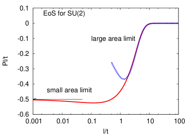
Figure 1: The equation of state for SU(2) gauge theory on a two-dimensional torus is shown as the solid curve. The asymptotic values of $Pl/t$ at small area is -0.5. At very large area, $Pl/t$ behaves as $0.75\exp(-0.75l/t)l/t$, which is shown as the dotted curve. There is a cross-over between the two limits.

Expecting that the equipartition limit is given by

$$\frac{Pl}{t}=-\frac{N-1}{2}\quad\text{as}\quad l\to 0,$$ (6)

for all $N$, we define

$$Q(\alpha)\equiv-\frac{2Pl}{(N-1)t};\quad\text{with}\quad\alpha=\frac{Nl}{t},$$ (7)

and study this quantity in this paper.

II Summary of results

We will show the following results in this paper using a numerical simulation of the partition function in Eq. (1):

1. $Q(\alpha)$ falls on a universal curve as $N\to\infty$.

2. $Q(\alpha)$ goes to zero as $\alpha$ goes to infinity. This result implies that the pressure at infinite $N$ is zero for all $l$ at any $t$ as long as one takes $N\to\infty$ keeping $l$ and $t$ finite and is consistent with physics being independent of temperature and spatial extent in the infinite $N$ limit Gross and Witten (1980); Eguchi and Kawai (1982).

3. $Q(\alpha)$ goes to unity as $\alpha$ goes to zero. This limit is reached from a finite $l$ and $t$ only at finite $N$.

4. There is a cross-over point defined as a peak in the susceptibility,

   $$\chi=A\frac{\partial}{\partial A}Q=\alpha\frac{\partial}{\partial\alpha}Q.$$ (8)

   1. The large $l$ side of the cross-over is dominated by representations where $C^{\scriptscriptstyle{(2)}}_{r}$ are of $\mathscr{O}(N)$. This is the case of interest for all non-zero $l$ at infinite $N$ and studied in Gross and Taylor (1993).

   2. The small $l$ side of the cross-over is dominated by representations where $C^{\scriptscriptstyle{(2)}}_{r}$ are of $\mathscr{O}(N^{2})$.

5. Since the value of $Q$ at infinite $N$ and $l=0$ (or equivalently $t=\infty$) depends on the approach to the limit, $N\to\infty$ and $l\to 0$, there is a first order transition confirming the argument in McLerran and Sen (1985).

III Properties of Casimir for SU(N)

The representations of SU($N$) are specified by the sequence of integers $\Lambda_{r}=\left(\lambda_{1},\lambda_{2},\ldots,\lambda_{N-1}\right)$, subjected to the ordering $\lambda_{i}\geq\lambda_{i+1}$ and the value of $C^{\scriptscriptstyle{(2)}}_{r}$ is

$$C^{\scriptscriptstyle{(2)}}_{r}=\sum_{i=1}^{N-1}\lambda_{i}^{2}-\sum_{i=1}^{N-1}i\lambda_{i}-\frac{\lambda^{2}}{N}+(N+1)\lambda\quad\text{where}\quad\lambda=\sum_{i=1}^{N-1}\lambda_{i}.$$ (9)

The maximum and the minimum value of Casimir, given the constraint that $\lambda$ has to be kept fixed, would be used in the subsequent sections. The representation with the maximum value of $C^{\scriptscriptstyle{(2)}}_{r}$ for a given $\lambda$ is given by

$$\Lambda_{\rm max}=(\lambda,0,\ldots,0).$$ (10)

The minimum value of $C^{\scriptscriptstyle{(2)}}_{r}$ is given by the sequence $\Lambda_{\rm min}$:

$$\lambda_{i}=\left\{\begin{array}[]{ll}\lfloor\frac{\lambda}{N-1}\rfloor+1&\mbox{if }i\leq k\equiv\lambda-(N-1)\lfloor\frac{\lambda}{N-1}\rfloor\\ \lfloor\frac{\lambda}{N-1}\rfloor&\mbox{if }i>k.\end{array}\right.$$ (11)

To prove that the two sequences extremize the Casimir, note that the Casimir decreases under the transformation $(\lambda_{1},\lambda_{2},\ldots,\lambda_{i},\ldots,\lambda_{j},\ldots,\lambda_{N-1})$ to $(\lambda_{1},\lambda_{2},\ldots,\lambda_{i}-1,\ldots,\lambda_{j}+1,\ldots,\lambda_{N-1})$ for $j>i$, provided this transformation is allowed. Such a transformation is not possible for $\Lambda_{\rm min}$. Similarly, the reverse of that transformation is not possible on $\Lambda_{\rm max}$. One can prove by contradiction that $\Lambda_{\rm min}$ and $\Lambda_{\rm max}$ are unique to satisfy these properties.

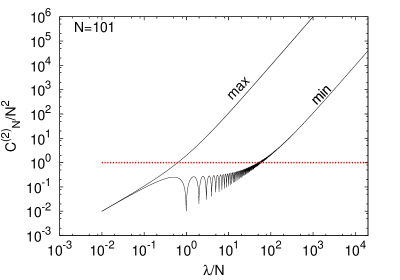
Figure 2: Behaviour of Casimir as a function of $\lambda$. The upper solid curve is the maximum value of Casimir given a value of $\lambda$, as a function of $\lambda$. Similarly, the lower solid curve is the minimum value of Casimir given a value of $\lambda$, as a function of $\lambda$. The dotted line is where $C^{\scriptscriptstyle{(2)}}_{r}=N^{2}$.

We have shown the behaviour of the maximum and the minimum value of $C^{\scriptscriptstyle{(2)}}_{r}$ as a function of $\lambda$ in Figure 2. The minimum of $C^{\scriptscriptstyle{(2)}}_{r}$ shows a quasi-periodic behaviour, with troughs at $\lambda=qN$ for integer $q$. The values of Casimir at these troughs are

$$C_{\rm min}=N\left(1+\left\lfloor\frac{q}{N-1}\right\rfloor\right)\left(2q-\left\lfloor\frac{q}{N-1}\right\rfloor(N-1)\right),$$ (12)

whose dependence on $N$ is linear for $q$ between two multiples of $(N-1)$ and is quadratic for $q$ that are multiples of $(N-1)$. On very large circles (or at very low temperatures), one would expect that only the excitations around these troughs at small $q$ would be important. On very small circles (or at very high temperatures), large values of $q$ would become accessible, where all possible Casimir are $\mathscr{O}(N^{2})$. This is the region above the red dotted line in Figure 2 where $C^{\scriptscriptstyle{(2)}}_{r}$ is larger than $N^{2}$. Qualitatively, this is the difference one might expect between the low and high temperature phases.

IV Heat-bath algorithm

We simulated the partition function in Eq. (1) by updating $\Lambda_{r}$ by the heat-bath algorithm. Each heat-bath update is a sequence of local updates from $\lambda_{1}$ to $\lambda_{N-1}$, in that order, such that the ordering of $\lambda_{i}$ is preserved. For the local update of $\lambda_{i}$, the probability distribution of $\lambda_{i}$ is given by a discrete version of the Gaussian distribution

$$T\left(\lambda_{i}\right)\propto e^{-(\lambda_{i}-\mu_{i})^{2}/2\sigma^{2}},$$ (13)

subject to the condition $\lambda_{i+1}\leq\lambda_{i}\leq\lambda_{i-1}$ for $i>1$ and $\lambda_{2}\leq\lambda_{1}$. The $\mu_{i}$ and $\sigma_{i}$ for the above discrete Gaussian distribution are functions of the rest of the $\lambda_{i}$’s forming the heat-bath:

$$\mu_{i}=\frac{\overline{\lambda}+N\left(\frac{2i-N-1}{2}\right)}{N-1}\quad\text{and}\quad\sigma^{2}=\frac{N^{2}}{2A\left(N-1\right)},$$ (14)

where $\overline{\lambda}=\sum_{j\neq i}\lambda_{j}$. For $i>1$, the set of allowed values for $\lambda_{i}$ is bounded from above and below. Hence, we included all the allowed possibilities weighted by Eq. (13) as candidates for the update. Since Eq. (14), along with the inequality $\lambda-\lambda_{1}<(N-2)\lambda_{2}$, implies that $\mu_{1}<\lambda_{2}$, the probability for $\lambda_{1}$ is a monotonically decreasing function. This enables one to put an upper cut-off on $\lambda_{1}$. In our calculation, we used an upper cut-off of $\lambda_{2}+3\sigma$. We also checked that changing this value to $\lambda_{2}+10\sigma$ does not cause any statistically significant changes. Since a representation $r$ and its conjugate representation $\overline{r}$ have the same Casimir, one can do an over-relaxation step by a global update $\lambda^{\prime}_{i}=\lambda_{1}-\lambda_{N-i+1}$.

In our simulations, the successive measurements were separated by 100 iterations of 2 heat-bath and 1 over-relaxation steps. The first 2000 measurements were discarded for thermalization. In this way, we collected $10^{4}$ configurations of $\Lambda_{r}$ at all area and $N$.

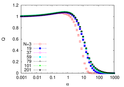
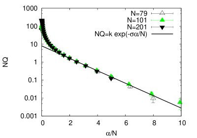
Figure 3: $Q$ as a function of the scaled area $\alpha=NA$ is shown in the top panel. It is seen that $Q$ as a function of $\alpha$ has a large-$N$ limit. For very small values of $\alpha$, $Q$ approaches $1$. In the bottom panel, the large area behaviour of $Q$ in the large-$N$ limit is shown. In this case, $QN$ behaves as $\exp\left(-\sigma\alpha/N\right)$.

V Results

In the top panel of Figure 3, we show the behaviour of $Q$ as a function of the scaled area $\alpha$ for various values of $N$. The important thing to notice is that $Q$ has a large-$N$ limit when plotted as a function of $\alpha$. For $\alpha\ll 1$, $Q$ seems to approach $1$ for all $N$. This is in agreement with our intuition based on the equipartition theorem. The non-trivial observation is that this cross-over to the equipartition limit happens at a finite value of $\alpha$ in the large-$N$ limit. For $\alpha\gg 1$, $Q$ seems to behave as $N^{-1}\exp\left(-\sigma\alpha/N\right)$ for a constant $\sigma\approx 0.81$ in the large-$N$ limit. This is shown in the bottom panel of Figure 3. Thus, it can also be seen as a cross-over from strong-coupling regime, which has a scale $\sigma$, to the weak-coupling regime with no underlying scale.

We determined the cross-over point $\alpha_{c}$ using the peak-position of the susceptibility $\chi$, after interpolating using multi-histogram reweighting. We show $\chi$ as a function of $\alpha$ in Figure 4 for various $N$. The susceptibility also has a large-$N$ limit when plotted as a function of $\alpha$. The peak positions of susceptibility for $N>19$ agree within errors, giving us an estimate $\alpha_{c}=12.1(2)$. This implies that the cross-over area $A_{c}=\alpha_{c}/N$ shifts to smaller values at larger $N$. The width of the susceptibility when expressed in terms of the area $A$ decreases inversely as $N$. This is characteristic of finite volume scaling near a first order phase transition, with the large-$N$ limit replacing the thermodynamic limit in this case.

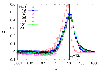
Figure 4: Susceptibility $\chi$ as a function of the scaled area $\alpha=NA$. The cross-over coupling $\alpha_{c}$ is shown by the vertical line.

The reason for this cross-over can be understood from the scatter plot of $C^{\scriptscriptstyle{(2)}}_{r}$ versus $\lambda$ measured during the course of the Monte Carlo run using a value of $\alpha$. Such scatter plots at various $\alpha$ are shown in Figure 5 for two different $N$. We also show the maximum and minimum value of Casimir at a fixed $\lambda$, as a function of $\lambda$. As discussed earlier, the minimum Casimir shows a quasi-periodic behaviour forming wells with a periodicity $N$. At large values of $\alpha$, the representations near the troughs of these wells at small values of $\lambda$ get populated. The representations within these wells are sparse, and this discreteness govern the large area behaviour. At very small area, the most probable $C^{\scriptscriptstyle{(2)}}_{r}$ moves away from the line of minimum $C^{\scriptscriptstyle{(2)}}_{r}$ and remains in a region where one can approximate the distribution of Casimir by a continuum. The cross-over between the two behaviours is what shows up as a peak in $\chi$. As discussed in Section III, the Casimir near the troughs at small $\lambda$ is of $\mathscr{O}(N)$, while the Casimir at very large $\lambda$ is of $\mathscr{O}(N^{2})$. As shown by the dotted line in Figure 5, this cross-over at $\alpha\approx 12.1$ roughly occurs when the dominant behaviour $C^{\scriptscriptstyle{(2)}}_{r}$ changes from $\mathscr{O}(N)$ to $\mathscr{O}(N^{2})$.

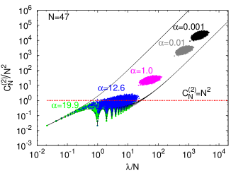
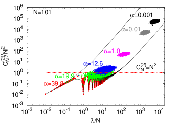
Figure 5: Scatter plot of $C^{\scriptscriptstyle{(2)}}_{r}/N^{2}$ versus $\lambda/N$ at various area $A$. The top panel is for $N=47$ and the bottom one for $N=101$. Each point corresponds to a $C^{\scriptscriptstyle{(2)}}_{r}$ and $\lambda$ measured in the course of Monte Carlo simulation at a particular $\alpha$ specified by the color. The upper and lower solid curves are the maximum and the minimum value of $C^{\scriptscriptstyle{(2)}}_{r}$ at a given $\lambda$ respectively.

VI Conclusions

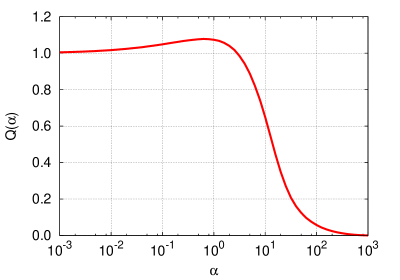
Figure 6: The large-$N$ limit of $Q$ as a function of $\alpha$.

Yang-Mills theory in two dimensions is always in the confined phase. We focused on the quantity, $Q=-\frac{2Pl}{(N-1)t}$, to study the equation of state. We showed that the equation of state shows a cross-over from strong coupling (large spatial extent) to weak coupling (small spatial extent) within the confined phase. Viewed as a function of $\alpha=\frac{lN}{t}$, $Q(\alpha)$ approaches a universal curve as $N\to\infty$ as shown in Figure 6. This behavior is similar to the Durhuus-Olesen transition Durhuus and Olesen (1981); Narayanan and Neuberger (2007) with the double scaling limit for the equation of state being $N\to\infty$ and $l\to 0$ (or $t\to\infty$) keeping $\alpha=\frac{lN}{t}$ fixed. There is a line of cross-over, $\frac{lN}{t}=\alpha_{c}$, extending from the origin in the $\frac{l}{t}$ – $\frac{1}{N}$ diagram as shown in Figure 7. Well above this line, $Q\ll 1$ and it behaves as $\exp(-\sigma A)/N$. Well below this line, $Q$ is approximately $1$. Depending on the slope, $\alpha$, of the line along which the $N\rightarrow\infty$ and $\frac{l}{t}\rightarrow 0$ limit is taken, the limiting value of $Q$ differs. Specifically, if $N\rightarrow\infty$ limit is taken after the $A\rightarrow 0$ limit is taken, then $Q$ is 1. When the two limits are reversed, $Q$ becomes 0. Therefore, the cross-over along $AN=\alpha_{c}$ becomes a first order transition at vanishing area in the large-$N$ limit.

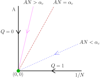
Figure 7: Phase diagram. Various approaches to vanishing area at large-$N$ are indicated by lines with arrows. The critical value of the slope $AN=\alpha_{c}$ is shown as the dot-dashed line. For values of $AN\gg\alpha_{c}$ (the dotted line), $Q$ decays exponentially with area. For values of $AN\ll\alpha_{c}$ (the dashed line), $Q\approx 1$. In particular, when $A$ is reduced to $0$ after taking the large-$N$ limit (i.e., along $y$-axis), $Q$ vanishes. When the two limits are interchanged (i.e., along $x$-axis), $Q$ becomes $1$.

The equation of state in four dimensional Yang-Mills theories for several different values of $N$ has been recently studied Datta and Gupta (2010). The pressure is found to be close to zero in the confined phase. In light of this paper, it would be interesting to perform a careful study of the equation of state in the confined phase in three and four dimensions and see if one can see a cross-over similar to the one seen here in two dimensions.