Three-dimensional Atmospheric Circulation of Warm and Hot Jupiters: Effects of Orbital Distance, Rotation Period, and Non-Synchronous Rotation

Abstract

Efforts to characterize extrasolar giant planet (EGP) atmospheres have so far emphasized planets within 0.05 AU of their stars. Despite this focus, known EGPs populate a continuum of orbital separations from canonical hot Jupiter values (0.03-0.05 AU) out to 1 AU and beyond. Unlike typical hot Jupiters, these more distant EGPs will not generally be synchronously rotating. In anticipation of observations of this population, we here present three-dimensional atmospheric circulation models exploring the dynamics that emerge over a broad range of rotation rates and incident stellar fluxes appropriate for warm and hot Jupiters. We find that the circulation resides in one of two basic regimes. On typical hot Jupiters, the strong day-night heating contrast leads to a broad, fast superrotating (eastward) equatorial jet and large day-night temperature differences. At faster rotation rates and lower incident fluxes, however, the day-night heating gradient becomes less important, and baroclinic instabilities emerge as a dominant player, leading to eastward jets in the midlatitudes, minimal temperature variations in longitude, and, often, weak winds at the equator. Our most rapidly rotating and least irradiated models exhibit similarities to Jupiter and Saturn, illuminating the dynamical continuum between hot Jupiters and the weakly irradiated giant planets of our own Solar System. We present infrared (IR) light curves and spectra of these models, which depend significantly on incident flux and rotation rate. This provides a way to identify the regime transition in future observations. In some cases, IR light curves can provide constraints on the rotation rate of non-synchronously rotating planets.

1. Introduction

Ever since their initial discovery, the atmospheric structure and circulation of hot Jupiters has been a subject of intense focus. Light curves and secondary eclipse measurements have now been obtained for a variety of objects, constraining the three-dimensional temperature structure, day-night heat transport, and circulation regime. This observational vanguard has motivated a growing body of modeling studies of the three-dimensional atmospheric circulation of hot Jupiters (e.g. Showman & Guillot, 2002; Cooper & Showman, 2005; Dobbs-Dixon & Lin, 2008; Dobbs-Dixon & Agol, 2013; Showman et al., 2009, 2013a; Menou & Rauscher, 2010; Lewis et al., 2010; Heng et al., 2011b; Thrastarson & Cho, 2010; Perna et al., 2012; Rauscher & Kempton, 2014; Mayne et al., 2014). Most of these models have emphasized synchronously rotating hot Jupiters in $\sim$2–4-day orbits with properties similar to HD 189733b or HD 209458b.

Despite the focus of modeling efforts on HD 189733b-like and 209458b-like planets, groundbased surveys and the CoRoT and Kepler missions have greatly expanded the catalog of known extrasolar giant planets (EGPs) to include many Jupiter-sized objects outside the close-in hot-Jupiter population. Known EGPs populate nearly a continuum of orbital separations from canonical hot-Jupiter values ($\sim$0.03–0.05 AU) out to 1 AU and beyond. As we will show, for Jupiter-like tidal $Q$ values of $\sim$$10^{5}$, planets beyond $\sim$0.2 AU have tidal spindown times comparable to typical system ages, implying that these more distant EGPs will not in general be synchronously rotating. Depending on tidal $Q$ values, orbital histories, and other factors, even some planets inward of $\sim$0.1–0.2 AU may rotate asychronously. In anticipation of observations of this wider population, there is thus a strong motivation to explore the atmospheric circulation of hot and warm Jupiters over a wide range of incident stellar fluxes and rotation rates.

To date, however, no such systematic investigation has been carried out. Showman et al. (2009) and Rauscher & Kempton (2014) explored the effects of factor-of-two deviations from synchronous rotation in models of HD 189733b and/or HD 209458b. Lewis et al. (2014) performed an analogous study for the eccentric hot Jupiter HAT-P-2b. Kataria et al. (2013) performed a thorough parameter study of the effect of eccentricity and stellar flux on the circulation of eccentric hot Jupiters, considering both synchronous and pseudo-synchronous rotation rates. There has been no comparably thorough exploration isolating how both widely varying stellar flux and rotation rate affect the circulation for hot Jupiters on circular orbits.

Such a study can address fundamental questions on the mechanisms controlling hot-Jupiter atmospheric circulation and their relationship to the dominant circulation mechanisms of Solar-System planets such as Earth and Jupiter. Most models of synchronously rotating hot Jupiters in $\sim$3-day orbits predict significant day-night temperature contrasts and several broad zonal jets, including an eastward (superrotating) jet at the equator, which in some cases causes an eastward displacement of the hottest regions from the substellar longitude (e.g., Showman & Guillot, 2002). Showman & Polvani (2011) showed that many features of this circulation regime, including the equatorial superrotation, can be understood in terms of the interaction of standing, planetary-scale waves with the mean flow. However, it is unknown whether this circulation regime should apply across the range of hot and warm Jupiters or whether it should give way to other circulation regimes under greatly different conditions. Earth, for example, exhibits significant equator-to-pole temperature differences, only modest variations of temperature in longitude, and zonal winds that peak in midlatitudes, with westward zonal-mean flow in the equatorial troposphere. Such a regime, if it occurred on a close-in EGP, could lead to very different lightcurves and spectra than would otherwise occur.

Here, we present new three-dimensional circulation models over a broad range of rotation rates and incident stellar fluxes comparable to and less than that received by HD 189733b with the aim of understanding the conditions under which transitions to different circulation regimes occur, establishing the link to more Earth-like and Jupiter-like regimes, and determining the implications for observables. Section 2 presents theoretical arguments anticipating a transition in the circulation regime for warm and hot Jupiters. Section 3 presents our dynamical model used to test these ideas. Section 4 describes the basic circulation regimes of our model integrations, including a diagnosis of the conditions under which regime transitions occur. Section 5 presents more detailed diagnostics illuminating the dynamical mechanisms. Section 6 presents light curves and spectra that our models would imply. Our summary and conclusions are in Section 7.

2. Background theory and prediction of a regime transition

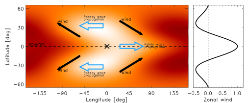
Figure 1.— Two regimes of atmospheric circulation of warm/hot Jupiters as proposed in this study. The top row, (a), represents the “canonical” hot Jupiter regime of slowly rotating, highly irradiated planets. The strong day-night thermal forcing induces significant day-night temperature differences and planetary-scale Kelvin and Rossby wave modes, which exhibit phase tilts that cause momentum to be transported to the equator. The result is a strong eastward (superrotating) jet at the equator. The bottom row, (b), is a regime we hypothesize to occur on warm Jupiters when the rotation is sufficiently fast and/or the stellar irradiation is sufficiently weak. In this case, the day-night forcing (i.e., the diurnal cycle) is relatively unimportant, and the circulation is instead driven by the zonal-mean, equator-to-pole contrast in stellar heating. Longitudinal temperature variations are small, but latitudinal temperature gradients (from equator to pole) can be large. In such a configuration, the midlatitudes can become baroclinically unstable, and the Rossby waves so generated cause momentum transport into the instability latitude, leading to the generation of “eddy driven” zonal jets. Zonal winds peak in the midlatitudes rather than the equator. The cross marks the substellar point.

Circulation models of “typical” hot Jupiters—defined here as those in several-day orbits with effective temperatures of 1000–$1500\rm\,K$ such as HD 189733b and HD 209458b—generally exhibit a circulation pattern near the infrared (IR) photosphere dominated by a fast, broad eastward jet centered at the equator (equatorial “superrotation”) and large temperature differences between the dayside and nightside (e.g. Showman & Guillot, 2002; Cooper & Showman, 2005; Showman et al., 2008, 2009, 2013a; Heng et al., 2011b, a; Perna et al., 2012; Rauscher & Menou, 2010, 2012a, 2013; Dobbs-Dixon & Lin, 2008; Dobbs-Dixon & Agol, 2013; Rauscher & Kempton, 2014). The day-night temperature differences in these models reach $\sim$200–$1000\rm\,K$ depending on pressure and on how the day-night thermal forcing is introduced. In many cases, the equatorial jet induces an eastward displacement of the hottest regions from the substellar point. Models that include radiative transfer show that IR lightcurves exhibit large flux variations with orbital phase, with a flux peak that often occurs before secondary eclipse (Showman et al., 2009; Heng et al., 2011a; Rauscher & Menou, 2012a; Perna et al., 2012; Dobbs-Dixon & Agol, 2013). Observational support for this dynamical regime comes from the overall agreement between observed and synthetic light curves and spectra—including inferences of eastward hotspot offsets—for HD 189733b (Showman et al., 2009; Knutson et al., 2012; Dobbs-Dixon & Agol, 2013), HD 209458b (Zellem et al., 2014), WASP-43b (Stevenson et al., 2014; Kataria et al., 2014b), and HAT-P-2b (Lewis et al., 2013, 2014). Eastward offsets have also been inferred on WASP-12b (Cowan et al., 2012) and Ups And b (Crossfield et al., 2010), although 3D models of those planets have yet to be published.

Showman & Polvani (2011) showed that the key dynamical feature of this circulation regime—the superrotating equatorial jet—results from a wave-mean-flow interaction caused by the strong day-night heating contrast. Figure 1a schematically illustrates this mechanism. The day-night heating contrast induces standing planetary-scale waves. In particular, a Kelvin wave is generated at low latitudes; it is centered about and exhibits thermal maxima occurring at the equator. Kelvin waves exhibit (group) propagation to the east, and in the context of a continuously forced and damped circulation, this leads to a quasi-steady, eastward displacement of the thermal pattern at the equator (Figure 1a, left). Moreover, equatorially trapped Rossby waves are generated on the poleward flanks of the Kelvin wave. These waves exhibit group propagation to the west, and in the presence of continuous thermal forcing and damping, a quasi-steady westward displacement of the thermal pattern emerges at mid-latitudes (Figure 1a, left). This latitudinally varying zonal phase shift implies that the thermal and eddy wind structure exhibits northwest-southeast tilts in the northern hemisphere and southwest-northeast tilts in the southern hemisphere. In turn, this eddy pattern induces a transport of eddy momentum from the midlatitudes to the equator, leading to equatorial superrotation (Figure 1a, right). See Showman & Polvani (2010, 2011), Showman et al. (2013a), and Tsai et al. (2014) for additional discussion; a review can be found in Showman et al. (2013b).

But theory and simulations from the solar-system literature indicate that, at sufficiently fast rotation and weak irradiation, the dynamics should shift to a different regime. When the irradiation is sufficiently weak, the day-night thermal forcing (i.e., the diurnal cycle) lessens in importance and the latitudinal variation of the zonal-mean heating becomes the dominant driver of the circulation. This heating pattern leads to significant temperature gradients in latitude but only small temperature gradients in longitude. Dynamical (e.g., thermal wind) balance requires that these meridional temperature gradients will be accompanied by strong zonal flow. A large body of work shows that, when the rotation is sufficiently fast, this configuration tends to be dynamically unstable: small perturbations in an initially zonally symmetric flow will grow via baroclinic instability, leading to baroclinic eddies that transport thermal energy poleward (for reviews see Pierrehumbert & Swanson 1995 or Vallis 2006, Chapter 6). Although such instability on Earth and Mars is enhanced by the existence of entropy gradients on the lower surface, several studies have shown that baroclinic instabilities are possible even on gas giants like Jupiter that lack such surfaces (Conrath et al., 1981; Read, 1988; Williams, 2003; Lian & Showman, 2008; O’Gorman & Schneider, 2008; Polichtchouk & Cho, 2012). Typically, such instabilities occur most readily at mid-to-high latitudes, where meridional temperature gradients are large and isentropes slope steeply. The thermal pattern expected in this regime is shown schematically in Figure 1b (left panel).

On rotating planets, because the gradient of the Coriolis parameter with northward distance, $\beta$, is nonzero, baroclinic instability can transport momentum from surrounding latitudes into the instability latitude, leading to the formation of so-called “eddy-driven” zonal jet streams at the instability latitude. Linear stability analyses demonstrate this transport in an idealized setting (e.g. Conrath et al., 1981; Held & Andrews, 1983; James, 1987), and nonlinear studies of forced-equilibrium circulations show how it can lead to the formation of zonal jets (Williams 1979, 2003; Panetta 1993; O’Gorman & Schneider 2008; Lian & Showman 2008, and many others). The process causing this momentum convergence is often described phenomenologically in terms of the excitation of Rossby waves at the instability latitude and their propagation to other latitudes where they dissipate or break (e.g., Held, 2000; Vallis, 2006). Rossby waves propagating northward from the instability latitude exhibit northward group velocity, whereas those propagating southward exhibit southward group velocity. Because Rossby waves with northward group velocity exhibit southward angular momentum transport, whereas those with southward group velocity exhibit northward angular momentum transport, the implication is that angular momentum is transported into the instability latitude from surrounding regions (Thompson, 1971; Held, 1975, 2000; Vallis, 2006; Showman et al., 2013b). To the extent that wave generation preferentially occurs at some latitudes, and wave breaking/dissipation in others, eddy-driven zonal jets will emerge in the midlatitudes, as shown schematically in Figure 1b (right panel).

Several eddy-mean-flow feedbacks promote the emergence of discrete midlatitude zonal jets (as opposed to simply broad strips of eastward wind) in this regime. When the zonal wind speeds increase with height, eastward jets tend to be more baroclinically unstable than westward jets; the former support a greater number of possible instability modes, and generally exhibit greater baroclinic instability growth rates, than the latter (e.g., Wang, 1990; Polichtchouk & Cho, 2012). This may allow preferential Rossby wave generation at eastward jets, thereby promoting preferential angular momentum transport into them. Perhaps more importantly, the breaking of Rossby waves tends to occur more readily in westward jets, where the meridional potential vorticity (PV) gradient is small, than it does in eastward jets, where the PV gradient is large. The meridional mixing caused by Rossby-wave breaking decreases still further the (already weak) PV gradient in westward jets, promoting even stronger Rossby wave breaking there. This is a positive feedback, which implies that, even if Rossby wave generation occurs randomly everywhere, the wave breaking—and associated PV mixing—will self-organize. The result tends to be series of zonal strips of nearly constant PV, with sharp PV jumps in between, which corresponds to the spontaneous emergence of zonal jets when the Rossby number is sufficiently small. See Dritschel & McIntyre (2008) or Showman et al. (2013b) for reviews.

Assembling these arguments, we thus predict a regime transition for warm/hot Jupiters as a function of stellar irradiation and rotation rate. When stellar irradiation is strong and the rotation rate is modest—as for synchronously rotating planets on several-day orbits—we expect large day-night temperature differences and strong equatorial superrotation—as shown in Figure 1a. When stellar irradiation is weak or the rotation rate is fast, we expect minimal longitudinal temperature differences, significant equator-pole temperature differences, midlatitude baroclinic eddies, and zonal-mean zonal winds that reach a maximum at the midlatitudes rather than the equator. These two regimes will have very different predictions for light curves, IR spectra, and Doppler signatures that may be detectable in observations.

What should be the criterion for the transition? Perez-Becker & Showman (2013) presented an analytic theory for the day-night temperature difference for synchronously rotating planets; however, no such theory yet exists for the more general case of non-sychronously rotating planets, especially when baroclinic instabilities become important. Nevertheless, a reasonable hypothesis is that the transition between these regimes should occur when the radiative time constant (e.g., at the photosphere) approximately equals the solar day. Here, the radiative time constant is the characteristic time for the atmosphere to gain or lose energy by radiation, and the solar day is the characteristic time (say) between two successive sunrises at a given point on the planet. When the radiative time constant is shorter than the solar day, the day-night (diurnal) forcing is strong, leading to wave-driven equatorial superrotation as shown in Figure 1a. When the radiative time constant is longer than the solar day, the diurnal cycle becomes dynamically less important than the meridional gradient in zonal-mean heating, and one obtains the regime of mid-latitude jets shown in Figure 1b. When winds are a significant fraction of the planetary rotation speed, the “solar day” should be generalized to include the zonal advection by winds.

Let us quantify this criterion. The solar day is $P_{\rm solar}=2\pi/|\Omega-n|$, where $n$ is the orbital mean motion (i.e., the mean orbital angular velocity). Thus,

$$P_{\rm solar}={1\over|{1\over P_{\rm rot}}-{1\over P_{\rm orb}}|}={1\over|{1\over P_{\rm rot}}-{1\over ka_{\rm orb}^{3/2}}|}$$ (1)

where $P_{\rm rot}=2\pi/\Omega$ is the (siderial) rotation period of the planet, $P_{\rm orb}$ is the orbital period, $a_{\rm orb}$ is the orbital semimajor axis, and in the second expression we have used Kepler’s 3rd law. Here, $k=2\pi/\sqrt{G(M_{*}+M_{p})}=3.46\times 10^{7}\rm\,s\,AU^{-3/2}$, where $G$ is the gravitational constant, $M_{*}$ and $M_{p}$ are the stellar and planetary masses, and we have evaluated the expression for HD 189733. To order of magnitude, the radiative time constant near the photosphere is (Showman & Guillot, 2002)

$$\tau_{\rm rad}={pc_{p}\over 4g\sigma T_{e}^{3}}$$ (2)

where $p$ is the pressure of the heated part of the atmosphere, $c_{p}$ is the specific heat at constant pressure, $g$ is gravity, $\sigma$ is the Stefan-Boltzmann constant, and $T_{e}$ is the planet’s equilibrium temperature. Assuming zero albedo, the latter can be expressed as $T_{e}=2^{-1/2}(R_{*}/a_{\rm orb})^{1/2}T_{*}$, where $R_{*}$ and $T_{*}$ are the stellar radius and temperature, respectively. Thus,

$$\tau_{\rm rad}\approx{pc_{p}\over g\sigma T_{*}^{3}}\left({a_{\rm orb}\over R_{*}}\right)^{3/2}$$ (3)

Equating this expression to the solar day, we obtain—as a function of of orbital semimajor axis and stellar properties—the planetary rotation period for which the solar day equals the radiative time constant

$$P_{\rm rot}\approx{1\over{1\over ka_{\rm orb}^{3/2}}+{g\sigma T_{*}^{3}\over pc_{p}}\left({R_{*}\over a_{\rm orb}}\right)^{3/2}}.$$ (4)

This expression assumes the rotation is prograde and faster than the orbital motion. Generalizing to include a constant equatorial zonal-wind speed $U$, the time between successive sunrises for a zonally circulating air parcel would become $P_{\rm solar}=2\pi/|\Omega+U/a-n|$, where $a$ is the planetary radius. Equating this expression to the radiative time constant yields the following generalized version of Equation (4):

$$P_{\rm rot}\approx{1\over{1\over ka_{\rm orb}^{3/2}}-{U\over 2\pi a}+{g\sigma T_{*}^{3}\over pc_{p}}\left({R_{*}\over a_{\rm orb}}\right)^{3/2}}.$$ (5)

We plot these expressions as a function of $P_{\rm rot}$ and $a_{\rm orb}$ in Figure 2, using an eastward wind $U=1\rm\,km\,s^{-1}$. Regions below the dashed line have $\tau_{\rm rad}<P_{\rm solar}$ and should exhibit the regime of large day-night temperature differences and equatorial superrotation shown in Figure 1a. Regions above the dashed line have $\tau_{\rm rad}>P_{\rm solar}$ and should exhibit the regime of mid-to-high-latitude jet and small zonal temperature variations of Figure 1b. Our simulations serve as a test of this prediction and will clarify the dynamics operating in each regime.

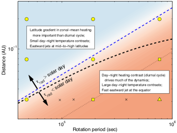
Figure 2.— Predicted phase diagram of dynamical regimes. Blue dashed line shows the planetary rotation rates and orbital semimajor axes at which the planet’s solar day equals its photospheric radiative time constant (Equation 4); black dashed line shows the same criterion generalized to include a constant eastward zonal wind of $U=1\rm\,km\,s^{-1}$ (Equation 5). Regions below the line (orange) have $\tau_{\rm rad}<P_{\rm solar}$ and should exhibit large-day night temperature differences with a fast eastward equatorial jet. Regions above the line (blue) exhibit $\tau_{\rm rad}>P_{\rm solar}$ and should have a circulation exhibiting mid-to-high latitude zonal jets with little zonal temperature variation. The equation is evaluated using $T_{*}=4980\rm\,K$ and $R_{*}=0.788R_{\odot}=5.5\times 10^{8}\rm\,m$ (appropriate to HD 189733), and $c_{p}=1.3\times 10^{4}\rm\,J\,kg^{-1}\,K^{-1}$ and $g=21\rm\,m\,s^{-2}$ appropriate to the planet. We adopt $p\approx 0.25\rm\,bar$, equivalent to that adopted by Perez-Becker & Showman (2013), who found a good fit between their model and lightcurve observations for hot Jupiters. Overplotted yellow symbols show the parameter combinations for GCM simulations presented in this paper; squares are synchronously rotating models, whereas circles (triangles) denote models whose rotation periods are shorter (longer) than their orbital periods. Crosses show non-synchronous models presented in Showman et al. (2009). Thin dotted line denotes synchronous rotation.

Although we focus here on this basic regime shift, it is worth emphasizing that the dynamics are complex and can exhibit richer behavior. In particular, each of the regimes (orange and blue) identified in Figure 2 could themselves split into several sub-regimes. For example, in the orange region, models in which the radiative time constant becomes particularly short—and/or the rotation rate becomes particularly long—could transition from a regime of fast equatorial superrotation to a regime where day-night flow dominates the circulation (e.g. Showman et al., 2013a). In the blue region, sufficiently rapid rotation should lead to a tropical zone confined near the equator, with a broad extratropical zone at mid-to-high latitudes in which baroclinic instabilities occur as depicted in Figure 1a. However, if the rotation rate is sufficiently slow (while still maintaining $\tau_{\rm rad}>P_{\rm solar}$), the planet may become an “all tropics” world with a global Hadley circulation in which baroclinic instabilities play a minimal role. While such a planet would still exhibit small zonal temperature variations and zonal winds peaking in midlatitudes, the dynamics controlling those jets may differ from the rapidly rotating case. Titan and Venus provide the best solar system analogues. This regime has been well studied for terrestrial planets (e.g., Del Genio & Suozzo, 1987; Del Genio & Zhou, 1996; Mitchell et al., 2006; Mitchell & Vallis, 2010; Kaspi & Showman, 2014) but has yet to receive attention for gas giants. Moreover, our considerations neglect any role for strong frictional drag, strong magnetic coupling, or strong internal convection, all of which may influence the dynamical regime.

3. Model

We solved the coupled hydrodynamics and radiative transfer equations using the Substellar and Planetary Atmospheric Radiation and Circulation (SPARC/MITgcm) model of Showman et al. (2009). This model solves the global, three-dimensionsal primitive equations in spherical geometry, with pressure as a vertical coordinate, using the MITgcm (Adcroft et al., 2004). The radiative transfer is solved using the two-stream variant of the multi-stream, non-grey radiative transfer model of Marley & McKay (1999). Opacities are treated using the correlated-$k$ method, which retains most of the accuracy of full line-by-line calculations but with dramatically reduced computational overhead. Opacities are treated statistically in each of 11 wavelength bins (see Kataria et al. 2013), allowing the inclusion of $10^{5}$ to $10^{6}$ individual opacity points within each bin; this is far more accurate than grey or multi-band approaches that adopt a single, mean opacity in each of a small number of wavelength bins (e.g., Rauscher & Menou 2012b, Heng et al. 2011a, Dobbs-Dixon & Agol 2013; see Amundsen et al. 2014 for a detailed discussion). To date, the SPARC model is the only general circulation model (GCM) that has been used to model the 3D circulation of hot Jupiters including a realistic representation of non-grey radiative transfer, as necessary for accurate assessment of the opacities, heating rates, and temperature structure under particular assumptions about the atmospheric composition. Gaseous opacities are determined assuming local chemical equilibrium (accounting for rainout of condensates) at a specified atmospheric metallicity. We have explored a variety of metallicities in prior work (Showman et al., 2009; Lewis et al., 2010), but as our emphasis here is on the dependence of the circulation regime on irradiation and rotation rate, we adopt solar metallicity for the current work. We neglect any opacity due to clouds or hazes. The radiative-transfer model adopts at the base an internal radiative heat flux of $5\rm\,W\,m^{-2}$, similar to that expected for generic multi-Gyr-old hot Jupiters (e.g., Guillot & Showman 2002, Fortney et al. 2007, and others). Nevertheless, this plays little role in the dynamics on the timescale of these simulations, as the absorbed stellar flux exceeds this intrinsic flux by a factor ranging from hundreds to $>10^{4}$, depending on the model.

Treating HD 189733b as a nominal case, we vary the the orbital semimajor axis and rotation rate over a large range. We explore orbital semimajor axes of 0.0313 AU (the actual value for HD 189733b), 0.0789 AU, and 0.1987 AU, corresponding to stellar fluxes incident on the planet of $4.68\times 10^{5}$, $7.37\times 10^{4}$, and $1.16\times 10^{4}\rm\,W\,m^{-2}$, respectively. This corresponds to a significant variation—greater than a factor of 40 in stellar flux—while still emphasizing close-in planets amenable to transit observations.

The rotation periods of hot Jupiters are often assumed to be synchronous with their orbital periods (Guillot et al., 1996; Rasio et al., 1996). The spindown timescale from a primordial rotation rate $\Omega_{p}$ is

$$\tau\sim Q\left({R_{p}^{3}\over GM_{p}}\right)\Omega_{p}\left({M_{p}\over M_{\star}}\right)^{2}\left({a_{\rm orb}\over R_{p}}\right)^{6}$$ (6)

where $Q$, $R_{p}$ and $M_{p}$ are the planet’s tidal dissipation factor, radius and mass, $G$ is the gravitational constant, $a_{\rm orb}$ is the orbital semimajor axis (here considering a circular orbit), and $M_{\star}$ is the mass of the star. Adopting a solar mass for the star, a Jupiter mass for the planet, and taking the planetary radius as 1.2 Jupiter radii (typical for a hot Jupiter), we obtain

$$\tau\sim 1\times 10^{6}\left({Q\over 10^{5}}\right)\left({a_{\rm orb}\over 0.05{\rm AU}}\right)^{6}\,{\rm yr}.$$ (7)

For a Jupiter-like $Q\sim 10^{5}$, this yields $\tau\sim 10^{6}\,$yr for canonical hot-Jupiter orbital separations of 0.05 AU, but the timescale increases to $4\times 10^{9}\rm\,yr$—comparable to typical system ages—for orbital separations of 0.2 AU. Thus, while this argument suggests that hot Jupiters should be tidally locked inward of 0.05 AU, sychronization should not be expected outward of 0.2 AU, and at intermediate distances (perhaps for planets that have experienced only a few spindown times), the planet may have been significantly despun but not yet become fully synchronized. Note that tidal $Q$ values are highly uncertain, and planet radii vary over a wide range from $\sim$1–2 Jupiter radii, implying that the orbital semimajor axes over which synchronization is expected are uncertain and may vary from system to system. Moreover, it has been suggested, even when Eq. (6) predicts synchronization, that in some cases the gravitational torque on not only the gravitational tide but also on the thermal tidal response may be important, leading to an equilibrium configuration with asychronous rotation (Showman & Guillot, 2002; Arras & Socrates, 2010).

Motivated by these considerations, we explore rotation periods varying by up to a factor of four from the nominal orbital period of HD 189733b, that is, 0.55, 2.2, and 8.8 Earth days, corresponding to rotation rates $\Omega$ of $1.322\times 10^{-4}\rm\,s^{-1}$, $3.3\times 10^{-5}\rm\,s^{-1}$, and $8.264\times 10^{-6}\rm\,s^{-1}$. The shortest of these is close to Jupiter’s rotation period of 10 hours. This is a wider exploration of rotation rate than considered in previous studies of non-synchronous rotation (Showman et al., 2009; Kataria et al., 2013; Rauscher & Kempton, 2014; Lewis et al., 2014). In our non-synchronous models, the longitude of the substellar point migrates in time $t$ as $(n-\Omega)t$, where $n$ is $2\pi$ over the orbital period; thus, in the reference frame of the rotating planet, the entire dayside heating pattern migrates east or west over time. We assume circular orbits with zero obliquity.

In total, these variations constitute a regular grid of models varying the rotation rate by a factor of 16 and the incident stellar flux by a factor of over 40. Figure 2 depicts the parameter space explored. For each integration, we denote the irradiation level by H for hot, W for warm, and C for cold (representing models with orbital semimajor axes of 0.03, 0.08, and $0.2\,$AU respectively) and rotation rate by $\Omega_{\rm fast}$, $\Omega_{\rm med}$, and $\Omega_{\rm slow}$. Thus for example H$\Omega_{\rm slow}$is the most highly irradiated, slowly rotating model, while C$\Omega_{\rm fast}$is the least irradiated, most rapidly rotating model.

All models adopt the radius and gravity of HD 189733b ($1.15R_{J}$ and $21.4\rm\,m\,s^{-2}$, respectively), $c_{p}=13000\rm\,J\,kg^{-1}\,K^{-1}$, a ratio of gas constant to specific heat at constant pressure $R/c_{p}=2/7$, and the ideal-gas equation of state. As is standard in GCMs, gravity and $R/c_{p}$ are assumed constant, which is a reasonably good approximation. The models are integrated from rest using an initial temperature-pressure profile from a one-dimensional planetwide-average radiative-equilibrium calculation. Liu & Showman (2013) showed the typical hot Jupiter regime does not exhibit significant sensitivity to initial conditions.

Our nominal grid of models do not include explicit frictional drag. The mechanisms of frictional dissipation in hot-Jupiter atmospheres are poorly understood and could include magnetohydrodynamic (ion) drag (Perna et al., 2010), vertical turbulent mixing (Li & Goodman, 2010), and breaking small-scale gravity waves (e.g., Lindzen, 1981). The atmospheres of planets in the Solar System are generally relatively inviscid except near the surfaces. In giant planets such as Jupiter, magnetohydrodynamic drag at great depth has been suggested as a key process in braking the interior winds (Kirk & Stevenson, 1987; Liu et al., 2008; Schneider & Liu, 2009). For hot Jupiters as cool as or cooler than HD 189733b, recent circulation models suggest that magnetic coupling is unimportant in the observable atmosphere (Rauscher & Menou, 2013; Rogers & Showman, 2014), although it may play a role in the deep atmosphere (pressures greater than tens to hundreds of bar) where temperatures become hot. Motivated by this possibility, we performed a range of sensitivity studies where we included frictional drag near the bottom of the model, where temperatures are warmest and magnetohydrodynamic braking is most likely.

We integrated each model until the velocities at low pressure reached a stable configuration. In the models without explicit large-scale drag, the winds in the observable atmosphere (pressures less than 0.1 bar) become essentially steady within $\sim$3000 days, and sometimes much less. The winds at depth (pressures exceeding 10 bars) are generally much weaker than photosphere winds. Any further increases in wind speed beyond our $\sim$3000–6000-day integration periods are likely to be modest and confined to pressures well below the mean photosphere, such that influences on lightcurves and spectra are modest. When drag is included in the deep atmosphere, it readily allows the total kinetic energy to equilibrate. If this drag is confined to pressures exceeding 10 bars, it has little effect on the overall circulation regime at the photosphere; if the drag extends to pressures as low as 1 bar it starts to influence the details of the photospheric circulation, although the overall qualitative trends identified in this paper are unaffected. Although this is reassuring, it is clear that the drag formulation is one of the greatest uncertainties in current EGP circulation models.

The equations are solved on the cubed-sphere grid (Adcroft et al., 2004). The cases at the longest two rotation periods (2.2 and 8.8 Earth days) adopt a horizontal resolution of C32 (i.e. $32\times 32$ finite-volume cells on each cube face), corresponding to an approximate global resolution of $128\times 64$ in longitude and latitude. Because of the smaller Rossby deformation radius in the cases with shortest rotation period (0.55 days), the dominant lengthscales are smaller, and so we integrated all of these cases at C64 (i.e., $64\times 64$ cells on each cube face), corresponding to an approximate global resolution of $256\times 128$ in longitude and latitude. Nevertheless, the behavior of these high-resolution, rapidly rotating integrations is qualitatively similar to equivalent cases performed at C32 resolution. All models adopt a vertical grid containing $N_{r}=40$ levels. The bottom $N_{r}-1$ levels have interfaces that are evenly spaced in log-pressure between 0.2 mbar and 200 bar; the top level extends from 0 to 0.2 mbar. These models generally conserve total angular momentum to $\sim$0.02%.

4. Results: Basic circulation regime

Our key result is that the circulation undergoes a major reorganization as the irradiation level and rotation rate are varied—as predicted by the theoretical arguments in Section 2. At high irradiation and slow rotation rates, the circulation is dominated by a broad equatorial (superrotating) jet and significant day-night temperature differences at low pressure. But at low irradiation and/or faster rotation rates, the circulation shifts to a regime dominated by off-equatorial eastward jets, with weaker eastward or even westward flow at the equator; day-night temperature differences are smaller, and the primarily horizontal temperature differences instead occur between the equator and pole. This behavior emerges clearly in Figure 3, which presents the zonal-mean zonal wind versus latitude and pressure, and Figure 4, which shows the temperature and wind structure on the 170-mbar isobar, within the layer that shapes the IR light curves and spectra. Here, we discuss basic structure and trends across our entire ensemble, deferring to Section 5 more detailed diagnostics of the two regimes.

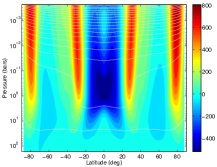
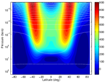
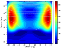
Figure 3.— Zonal-mean circulation for the nine runs in the nominal grid. Each panel plots zonal-mean zonal wind (colorscale, $\rm m\,s^{-1}$) and zonal-mean potential temperature (white contours) versus latitude and pressure. The left, middle, and right columns adopt rotation periods of 0.55, 2.2, and 8.8 days, respectively. The top, middle, and bottom rows adopt orbital semimajor axes of 0.2, 0.08, and 0.03 AU, respectively. Note the regime transition from a flow dominated by an equatorial superrotating jet in the bottom right (slow rotation, large incident flux) to a flow dominated by mid-latitude eastward jets in the middle and top left (fast rotation, small incident flux).

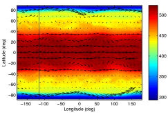
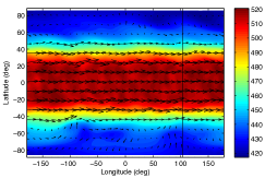
Figure 4.— Temperature (colorscale, K) and winds (arrows) on an isobar for the nine runs in the nominal grid. Each panel plots the temperature and winds versus longitude and latitude at 170 mbar. The left, middle, and right columns adopt rotation periods of 0.55, 2.2, and 8.8 days, respectively. The top, middle, and bottom rows adopt orbital semimajor axes of 0.2, 0.08, and 0.03 AU, respectively. Vertical black lines in each panel denote the substellar longitude at this snapshot. The hot cases tend to have large day-night temperature differences, especially at slow rotation rates; cooler cases—particularly at fast rotation rate—have minimal temperature differences in longitude but significant temperature differences in latitude.

First, consider the highly irradiated, slowly rotating regime of equatorial superrotation and large day-night temperature contrasts; this behavior is best developed in the lower-right corner of Figures 3–4 (models W$\Omega_{\rm slow}$, H$\Omega_{\rm med}$, and H$\Omega_{\rm slow}$). The circulation in this portion of the parameter space resembles that explored extensively in the hot Jupiter literature (e.g., Showman & Guillot, 2002; Showman et al., 2008, 2009; Dobbs-Dixon & Lin, 2008; Menou & Rauscher, 2009; Rauscher & Menou, 2010; Heng et al., 2011b). Peak zonal-mean zonal wind speeds reach 2 to $4\rm\,km\,s^{-1}$ in the core of the equatorial jet, with maximum wind speeds occurring at the equator. The jet extends smoothly from the top of the domain ($\sim$0.2 mbar) to a pressure of $\sim$3–10 bars depending on the model, with the fastest zonal-mean speeds at a midlevel of 0.1–0.3 bar. In models H$\Omega_{\rm med}$and H$\Omega_{\rm slow}$, the equatorial jet is sufficiently narrow for westward zonal-mean flow to develop at high latitudes; in others (W$\Omega_{\rm slow}$), the equatorial jet extends from pole to pole, such that the zonal-mean flow within the jet is eastward at essentially all latitudes. As shown in Figure 4, day-night temperature differences are large in the observable atmosphere. The dayside is characterized by a broad, hemispheric-scale hot region that is shifted eastward of the substellar longitude by $\sim$10–$50^{\circ}$ at the highest irradiation (H$\Omega_{\rm med}$and H$\Omega_{\rm slow}$) and $\sim$50–$90^{\circ}$ at lower irradiation (W$\Omega_{\rm slow}$). The amplitude of the offsets depend on pressure. Longitudinal temperature variations are up to $\sim$$400\rm\,K$ in the hottest models (H$\Omega_{\rm med}$and H$\Omega_{\rm slow}$) and $\sim$100–$200\rm\,K$ in W$\Omega_{\rm slow}$.

Next, consider the weakly irradiated and/or rapidly rotating regime (upper left portion of Figures 3–4; models C$\Omega_{\rm fast}$, C$\Omega_{\rm med}$, C$\Omega_{\rm slow}$, W$\Omega_{\rm fast}$, W$\Omega_{\rm med}$, and H$\Omega_{\rm fast}$). In this regime, superrotation is less dominant, and the circulation instead becomes dominated by eastward jets at mid-to-high latitudes in each hemisphere, with weaker eastward or even westward flow at the equator. Peak zonal-mean zonal wind speeds reach $\sim$0.6–$1.4\rm\,km\,s^{-1}$ in the off-equatorial eastward jets. When the rotation is slow-to-intermediate, only two off-equatorial eastward jets develop (one in each hemisphere), as seen in models C$\Omega_{\rm med}$, C$\Omega_{\rm slow}$, and W$\Omega_{\rm med}$. When the rotation is fast, however, the dynamical length scales are shorter, and the flow splits into four mid-latitude eastward jets (two per hemisphere), as in models H$\Omega_{\rm fast}$, W$\Omega_{\rm fast}$, and C$\Omega_{\rm fast}$. The phenomenon is best developed in model C$\Omega_{\rm fast}$, the fastest-rotating, lowest-irradiation model of our ensemble. In this regime, temperatures are relatively constant in longitude but vary significantly in latitude (middle and upper left of Figure 4). As can be seen from the detailed velocity patterns in Figure 4, the eastward mid-latitude jets exhibit quasi-periodic undulations in longitude with zonal wavenumbers ranging from 2 to $\sim$14, suggesting that the jets are experiencing dynamical instabilities. As we will show in Section 5, these instabilities play an important role in maintaining the jets. The off-equatorial ciculation in these models qualitatively resembles that of Earth or Jupiter.

The location of the transition, as a function of rotation rate and stellar flux, agrees well with that predicted in Section 2 (compare Figures 2 and 3). This provides tentative support for the theoretical arguments presented there.

The transition between the regimes is continuous and broad. Models along the boundary between the two regimes—in particular, C$\Omega_{\rm med}$, W$\Omega_{\rm med}$, and H$\Omega_{\rm fast}$—exhibit aspects of both regimes. For example, C$\Omega_{\rm med}$and W$\Omega_{\rm med}$exhibit a flow comprising midlatitude eastward jets (red colors in Figure 3) embedded in a broad superrotating flow that includes the equator. It is likely that, in this regime, diurnal (day-night) forcing and baroclinic instabilities both play a strong role in driving the circulation, leading to a hybrid between the two scenarios shown in Figure 1.

The importance of rotation in the dynamics varies significantly across our ensemble. This is characterized by the Rossby number, $Ro=U/\Omega L$, giving the ratio of advective to Coriolis forces in the horizontal momentum equation, where $U$ and $L$ are the characteristic wind speed and horizontal length scale and $\Omega$ is the planetary rotation rate. Considering a length scale $L\approx 10^{8}\rm m$ appropriate to a global-scale flow, our slowest-rotating models have $Ro=1.2(U/1000\rm\,m\,s^{-1})$, implying Rossby numbers as high as $\sim$4 when irradiation is strongest. In this case, Coriolis forces, while important, will be subdominant to advection in the horizontal force balances. On the other hand, our most rapidly rotating models exhibit $Ro=0.15(U/\rm\,1000\,m\,s^{-1})$, where we have used $L\approx 5\times 10^{7}\rm\,m$ to account for the shorter flow length scales in those cases (Figure 3, left column). When irradiation is weakest, wind speeds are typically $\sim$$300\rm\,m\,s^{-1}$ (Figure 3), implying $Ro\sim 0.05$—smaller than the value on Earth. This implies that the large-scale flow is in approximate geostrophic balance—i.e., a balance between Coriolis and pressure-gradient forces in the horizontal momentum equation. Such a force balance is the dominant force balance away from the equator on most solar system planets (Earth, Mars, Jupiter, Saturn, Uranus, and Neptune). In terms of force balances, these models therefore resemble these solar system planets more than “canonical” hot Jupiters.

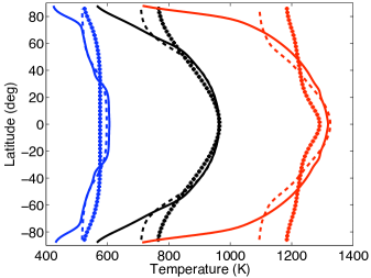
Figure 5.— Zonal-mean temperature versus latitude, averaged vertically from 60 mbar to 1 bar. Red, black, and blue curves represent models with strong, intermediate, and weak irradiations (i.e., H, W, and C respectively). Solid, dashed, and plus-sign curves denote models with fast, intermediate, and slow rotation ($\Omega_{\rm fast}$, $\Omega_{\rm med}$, and $\Omega_{\rm slow}$respectively). Model W$\Omega_{\rm fast}$has been averaged about the equator. At a given incident stellar flux, the equator-to-pole temperature difference increases with rotation rate; rapidly rotating models have warmer low-latitude regions and colder poles than slowly rotating models.

The rotation exerts a significant control over the temperature structure—faster rotation rates weaken the meridional (north-south) heat flux and lead to greater equator-to-pole temperature differences in the equilibrated state. Figure 5 shows the zonal-mean temperature versus latitude, averaged vertically between 60 mbar and 1 bar, for all nine nominal models. At a given incident stellar flux, rapidly rotating models exhibit colder poles and warmer mid-to-low-latitude regions than slowly rotating models. While all models exhibit net radiative heating at low latitudes and cooling at the poles, the temperatures shown in Figure 5 imply that the magnitude of this heating gradient is smaller in the rapidly rotating cases than the slowly rotating cases. Essentially, the rapid rotation acts to inhibit meridional heat transport, forcing the fluid to equilibrate to a state closer to the (latitudinally varying) radiative equilibrium temperature profile.

The tendency of rapidly rotating flows to exhibit larger horizontal temperature differences (Figure 5) can be understood with scaling arguments. The characteristic horizontal pressure-gradient force has magnitude $|\nabla\Phi|\sim R\delta T_{\rm horiz}\Delta\ln p/L$, where $R$ is the specific gas constant, $\delta T_{\rm horiz}$ is the characteristic horizontal temperature difference, and $\Delta\ln p$ is the range of log-pressures over which this horizontal temperature difference extends vertically (e.g., $\Delta\ln p=1$ if the temperature differences extend over a layer one scale height thick). Here, we consider the case where friction is weak, appropriate to most atmospheres (away from any solid surface) and to our simulations. In the slowly rotating regime, the pressure-gradient force is balanced primarily by advection, expressable to order-of-magnitude as $U^{2}/L$, where $U$ is a typical wind speed. On the other hand, in the rapidly rotating regime, the pressure-gradient force is balanced primarily by Coriolis forces, $\Omega U$. Writing the force balance for each of these cases, it follows that (Charney, 1963; Showman et al., 2013b)

$${\delta T_{\rm horiz}\over T}\approx\begin{cases}Fr&Ro\gtrsim 1,\\ {Fr\over Ro}&Ro\ll 1\end{cases}$$ (8)

where $Fr\equiv U^{2}/gH\Delta\ln p$ is a dimensionless number called a Froude number, which is the squared ratio of wind speed to a quantity related to the gravity wave speed; here, $H=RT/g$ is the atmospheric scale height and $g$ is gravity. The key point is that $\delta T_{\rm horiz}/T$ is significantly greater—by a factor $Ro^{-1}$—in the rapidly rotating regime than in the slowly rotating regime. Inserting numbers appropriate to our most strongly irradiated simulations ($U\approx 1000\rm\,m\,s^{-1}$, $g=23\rm\,m\,s^{-2}$, $H\approx 200\rm\,km$, $\Delta\ln p=2$) yields $\delta T_{h}\sim 100\rm\,K$ when rotation is slow but $\delta T_{h}\sim 600\rm\,K$ when rotation is fast. These values agree reasonably well with our simulation results (compare plus-sign and solid red curves in Figure 5).

The structure of isentropes—surfaces of constant entropy—differs considerably across our ensemble and provides important clues about the dynamical stability of the atmosphere. To show this, Figure 3 plots in contours the zonal-mean potential temperature for our simulations. Because the atmosphere is stably stratified throughout the domain, potential temperature increases upward. In our highly irradiated, slowly rotating models, zonal-mean isentropes are relatively flat (lower right corner of Figure 3), indicating that the zonal-mean temperature varies only modestly on constant-pressure surfaces (consistent with Figure 5). In our poorly irradiated and/or rapidly rotating models, however, the isentropes slopes becomes large in local regions. The slopes become particularly tilted at pressures of $\sim$0.1–1 bar and latitudes of $\sim$20–$40^{\circ}$ in our poorly irradiated models (C$\Omega_{\rm slow}$, C$\Omega_{\rm med}$, C$\Omega_{\rm fast}$), but the large slopes are confined closer to the poles in some other models (e.g., W$\Omega_{\rm fast}$and H$\Omega_{\rm fast}$). In some cases, individual isentropes vary in pressure by $\sim$3 scale heights over horizontal distances of only $\sim$$20^{\circ}$ latitude. In stratified atmospheres, sloping isentropes indicate a source of atmospheric potential energy that can be liberated by atmospheric motions. Strongly sloping isentropes—with vertical variations exceeding a scale height over horizontal distances comparable to a planetary radius—often indicate that the atmosphere is dynamically unstable, in particular to baroclinic instabilities. We return to this issue in Section 5.

5. Mechanisms

Here, we present further diagnostics that clarify the dynamical mechanisms occurring in each regime.

5.1. Slow rotation, high irradiation: equatorial superrotation

The slowly rotating, strongly irradiated regime of large day-night temperature differences and fast equatorial superrotation is exemplified by models H$\Omega_{\rm med}$, H$\Omega_{\rm slow}$, and W$\Omega_{\rm slow}$. As described in Section 2, Showman & Polvani (2011) showed that the day-night forcing generates standing, planetary-scale waves that transport angular momentum from mid-to-high latitudes to the equator, driving the equatorial superrotation.

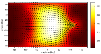
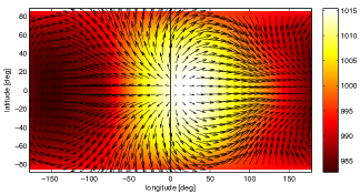
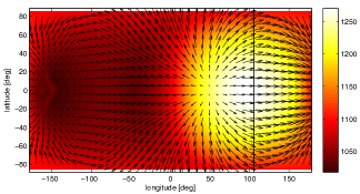
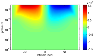
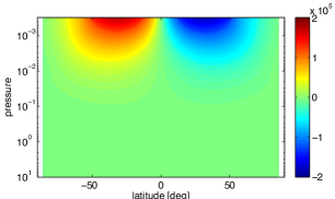
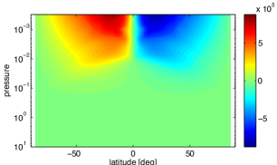
Figure 6.— Structure of our three highly irradiated, slowly rotating models during the spin-up phase, after the day-night heating contrast has induced a global wave response, but before strong zonal jets have developed. Models are H$\Omega_{\rm med}$(top), W$\Omega_{\rm slow}$(middle), and H$\Omega_{\rm slow}$(bottom) at times of 0.9, 1.4, and 0.9 Earth day, respectively. Left column shows temperature (colorscale, K) and winds (arrows) versus longitude and latitude on the 85-mbar level; right column shows zonal-mean meridional momentum transport, $\overline{u^{\prime}v^{\prime}}$, versus latitude and pressure. All three models show the development of a standing-wave, “Matsuno-Gill” pattern that causes a transport of angular momentum to the equator and subsequently generates equatorial superrotation. The solid lines in (a), (c), and (e) denote the substellar longitude. The top two rows are synchronously rotating models, whereas the bottom row exhibits asynchronous rotation.

Figure 6 demonstrates the existence of such a standing wave pattern in the transient spin-up phases of our highly irradiated, slowly rotating models. These are snapshots shown at early times, after the day-night forcing has had time to trigger a global wave response but before the equatorial jet has spun up to high speed. In synchronously rotating models H$\Omega_{\rm med}$and W$\Omega_{\rm slow}$, strong east-west divergence occurs along the equator from a point east of the substellar point (Figure 6a and c, respectively). At northern latitudes, Coriolis forces lead to clockwise curvature of the flow on the dayside and counterclockwise curvature on the nightside (with reversed directions at southern latitudes). Globally, these flows exhibit a striking similarity to the analytic standing-wave solutions of Showman & Polvani (2011, compare our Figures 6a and c to the top middle and top left panels of their Figure 3). The zonal divergence (with an eastward displacement) along the equator is precisely the behavior expected for a steady, forced, damped equatorial Kelvin wave, whereas the high-latitude behavior is analogous to the steady, forced, damped equatorial Rossby wave. Linear, analytic solutions show that the two wave components tend to be more distinct when the radiative or drag timescales are longer, and less distinct when they are shorter; the behavior in our simulations is toward the latter limit. In contrast, H$\Omega_{\rm slow}$(Figure 6e) is an asynchronous model where the substellar longitude migrates to the east over time. No analytic solutions of the asynchronous case have been published in the hot-Jupiter literature, but the similarity of the wind patterns to the synchronous case (particularly W$\Omega_{\rm slow}$) is evident. The main difference is that, although the thermal pattern tracks the heating (and is thus centered near the substellar longitude), there is a time-lag in the wind response, such that the flow divergence point lies west (rather than east) of the substellar point. Still, taken as a whole, Figure 6 provides strong evidence that the mechanism of Showman & Polvani (2011) is occurring in these simulations.

The planetary-scale waves shown in Figure 6 lead to a pattern of eddy velocities that transport angular momentum from the mid-latitudes to the equator, which allows the development of equatorial superrotation. This can be seen visually from the velocities in Figure 6 (left column), which exhibit a preferential northwest-southeast orientation in the northern hemisphere and southwest-northeast orientation in the southern hemisphere. As a result, one expects the eddy velocity correlation $\overline{u^{\prime}v^{\prime}}$ to be negative in the northern hemisphere and positive in the southern hemisphere, where $u$ and $v$ are the zonal and meridional winds, the primes denote deviations from the zonal average, and the overbar denotes a zonal average. This is explicitly demonstrated in Figure 6 (right column), which shows $\overline{u^{\prime}v^{\prime}}$ versus latitude and pressure for the three simulations in the left column. Note that $\overline{u^{\prime}v^{\prime}}$ represents the meridional transport of zonal (relative) momentum per unit mass by eddies (negative implying southward momentum transport and positive implying northward momentum transport). A strong equatorward momentum flux occurs at pressures less than 0.1 bar, with spatial patterns that are quite similar in all three cases. The momentum fluxes are largest in H$\Omega_{\rm med}$(Figure 6b) and somewhat smaller in H$\Omega_{\rm slow}$(Figure 6f), consistent with the fact that the eddy-velocity phase tilts are better correlated in the former than the latter. (That is, the eddy velocity tilts are more strongly organized in the poleward/westward to equatorward/eastward direction in H$\Omega_{\rm med}$than in H$\Omega_{\rm slow}$; the weaker correlation in H$\Omega_{\rm slow}$may result from the effect of slower rotation and/or non-synchronous rotation on the structure of the wave modes.) Model W$\Omega_{\rm slow}$exhibits the weakest momentum fluxes, presumably because of the weaker stellar forcing in that case.

More formally, the zonal-mean zonal momentum equation of the primitive equations using pressure as a vertical coordinate can be written

$${\partial\overline{u}\over\partial t}=\overline{v}\left[f-{1\over a\cos\phi}{\partial(\overline{u}\cos\phi)\over\partial\phi}\right]-\overline{\omega}{\partial\overline{u}\over\partial p}+\overline{X}$$

$$-{1\over a\cos^{2}\phi}{\partial(\overline{u^{\prime}v^{\prime}}\cos^{2}\phi)\over\partial\phi}-{\partial(\overline{u^{\prime}\omega^{\prime}})\over\partial p}$$ (9)

where $a$ is the planetary radius, $f=2\Omega\sin\phi$ is the Coriolis parameter, $\phi$ is latitude, $\omega=dp/dt$ is the vertical velocity in pressure coordinates (i.e., the rate of change of pressure with time following an air parcel), with $d/dt$ being the total (material) derivative in three dimensions, and $X$ represents any frictional terms. The terms on the righthand side represent meridional momentum advection by the mean flow, vertical momentum advection by the mean flow, frictional drag, horizontal convergence of eddy momentum, and vertical convergence of eddy momentum.

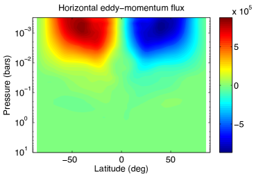
Figure 7.— Zonal eddy-momentum fluxes and convergences for our slowly rotating, highly irradiated model, H$\Omega_{\rm slow}$, averaged in time once the simulation has reached equilibrium at pressures less than a few bars. Panels (a) and (b) show the horizontal and vertical eddy fluxes, $\overline{u^{\prime}v^{\prime}}$ and $\overline{u^{\prime}\omega^{\prime}}$ (units of $\rm m^{2}\,s^{-2}$ and $\rm m\,Pa\,s^{-2}$ respectively). Panels (c) and (d) show the eddy-momentum convergences from Equation (9), $-(a\cos\phi)^{-1}\partial(\overline{u^{\prime}v^{\prime}}\cos^{2}\phi)/\partial\phi$ and $-\partial(\overline{u^{\prime}\omega^{\prime}})/\partial p$ (units of $\rm m\,s^{-2}$). Large-scale waves transport eddy momentum to equator and downward. Plots show the upper part of the domain from 0.3 mbar to 10 bars. Note that positive $\omega$ indicates downward motion, such that, in panel (b), a downward momentum flux is red, while an upward momentum flux is blue.

To illustrate how the thermally forced, planetary-scale waves maintain the equatorial jet, Figure 7 shows the resulting eddy fluxes and accelerations for our slowly rotating, highly irradiated model (H$\Omega_{\rm slow}$). These are long-time averages after the simulation has reached equilibrium at pressures less than a few bars. Panels (a) and (b) show the horizontal and vertical eddy fluxes, $\overline{u^{\prime}v^{\prime}}$ and $\overline{u^{\prime}\omega^{\prime}}$, whereas panels (c) and (d) show the eddy-momentum convergences from Equation (9), namely $-(a\cos\phi)^{-1}\partial(\overline{u^{\prime}v^{\prime}}\cos^{2}\phi)/\partial\phi$ and $-\partial(\overline{u^{\prime}\omega^{\prime}})/\partial p$. Planetary-scale waves transport eddy momentum to the equator (Figure 7a), especially at pressure less than $\sim$1 bar. At pressures less than $\sim$0.1 bar, this leads to a torque that causes an eastward acceleration at the equator and westward acceleration at high latitudes (Figure 7c), as expected from the arguments surrounding Figure 6 and from the theory of Showman & Polvani (2011). Indeed, the equilibrated, time-averaged meridional momentum fluxes shown in Figure 7a strongly resemble the structure and magnitudes of those at early times shown in Figure 6f. Considering now the vertical fluxes, Figure 7b shows that, at the equator, eddy momentum is transported downward from the upper regions ($\sim$1 mbar–1 bar) to pressures exceeding a few bars. This downward momentum transport induces a westward eddy acceleration at the equator, shown in panel (d), which largely cancels the eastward acceleration resulting from meridional momentum convergence. The residual eddy acceleration (sum of panels (c) and (d)) is very weakly eastward at the equator at most pressures, thereby maintaining the equatorial superrotation. Meanwhile, at high latitudes, the vertical eddy flux is upward (panel b), leading to an eastward eddy acceleration that largely cancels the westward eddy acceleration caused by the meridional convergence. In steady state, the net eddy acceleration—that is, the sum of the lower two panels in Figure 7—is balanced by a combination of Coriolis, horizontal mean advection, and vertical mean advection terms. At the equator, the Coriolis and horizontal mean advection terms are negligible, and the weak net eddy acceleration is balanced primarily by vertical advection (i.e., $-\overline{\omega}\partial\overline{u}/\partial p$).

The rotation rate and stellar heating pattern both exert significant control over the equatorial jet width. A comparison of models H$\Omega_{\rm med}$and W$\Omega_{\rm slow}$—which are both synchronously rotating—allows a comparison of the effects of rotation alone. Interestingly, W$\Omega_{\rm slow}$, which has a rotation rate four times slower than H$\Omega_{\rm med}$, exhibits an equatorial jet twice as wide, extending nearly from pole to pole (Figure 3). This agrees with the theory of Showman & Polvani (2011), which predicts for synchronously rotating planets that the meridional half-width of the equatorial jet is comparable to the equatorial Rossby deformation radius, $(NH/\beta)^{1/2}$, where $N$ is the Brunt-Vaisala frequency, $H$ is scale height, and $\beta=df/dy$ is the gradient of the Coriolis parameter with northward distance $y$. In contrast, a comparison of models W$\Omega_{\rm slow}$  and H$\Omega_{\rm slow}$  allows a comparison of stellar-heating pattern at constant rotation rate. Although the stellar insolation is fixed in longitude in W$\Omega_{\rm slow}$, it migrates eastward over time in H$\Omega_{\rm slow}$  due to the asynchronous rotation. Despite the identical rotation rates, the equatorial jet is much narrower in H$\Omega_{\rm slow}$than W$\Omega_{\rm slow}$. This suggests that the asynchronous thermal forcing alters the nature of the wave modes that are generated, leading to differing equatorial jet widths and speeds.

5.2. Fast rotation, weak irradiation: off-equatorial eastward jets

In comparison to the closest-in hot Jupiters, EGPs that are rapidly rotating and relatively far from their stars will exhibit relatively weak diurnal (day-night) forcing, and will exhibit a circulation that develops primarily in response to the need to transport heat from low to high latitudes. Here we describe the dynamics of this regime in further detail, focusing for concreteness on model C$\Omega_{\rm fast}$.

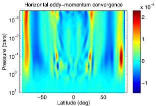
Figure 8.— Zonal-mean circulation diagnostics for model C$\Omega_{\rm fast}$, our coolest, most rapidly rotating model, averaged in time once the simulation has reached equilibrium at pressures less than a few bars. Panels (a) and (b) show the horizontal and vertical eddy-momentum convergence from Equation (9), $-(a\cos\phi)^{-1}\partial(\overline{u^{\prime}v^{\prime}}\cos^{2}\phi)/\partial\phi$ and $-\partial(\overline{u^{\prime}\omega^{\prime}})/\partial p$. Panel (c) shows their sum. (d) shows the Coriolis acceleration, $f\overline{v}$. The top four panels all have units $\rm m\,s^{-2}$. (e) shows the meridional eddy temperature flux, $\overline{v^{\prime}T^{\prime}}$ (units $\rm m\,K\,s^{-1}$), illustrating that large meridional eddy heat transport occurs across the eastward jets. (f) shows the zonal-mean streamfunction (black contours) overlain on the zonal-mean zonal wind (colorscale, $\rm m\,s^{-1}$). Solid is clockwise (with ten log-spaced contours between $1.3\times 10^{8}$ and $1.3\times 10^{13}\rm kg\,s^{-1}$) and dashed is counterclockwise (with ten log-spaced contours between $-1.3\times 10^{8}$ and $-1.3\times 10^{13}\rm kg\,s^{-1}$). White contours depict angular momentum per unit mass with respect to the planet’s rotation axis (with ten linearly spaced contours between $3.36\times 10^{10}$ and $8.99\times 10^{10}\rm m^{2}\,s^{-1}$).

In the rapidly rotating regime, the meridional heat transport is accomplished by baroclinic eddies that develop in the mid-to-high latitudes, which—as predicted by the theory in Section 2—transport momentum into their latitude of generation, thereby producing and maintaining the off-equatorial zonal jets that dominate this regime. Figure 8 illustrates this behavior for model C$\Omega_{\rm fast}$. Panels (a) and (b) show the time-mean, zonal-mean horizontal and vertical eddy momentum convergences, that is, the terms $-(a\cos^{2}\phi)^{-1}\partial(\overline{u^{\prime}v^{\prime}}\cos^{2}\phi)/\partial\phi$ and $-\partial(\overline{u^{\prime}\omega^{\prime}})/\partial p$, respectively from Equation (9). Figure 8c shows their sum. There is a strong correlation of the accelerations—particularly the horizontal eddy-momentum convergence—with the jet latitudes (compare Figure 8a and b to the zonal winds in Figure 3 or 8f). Specifically, the eddies produce strongest eastward accelerations primarily within the eastward jets, thereby maintaining them.

A mean-meridional circulation develops in response to the thermal and eddy forcing. This circulation organizes into a series of cells that extend coherently from the top of the domain ($\sim$0.2 mbar) to pressures exceeding 1 bar. The streamfunction $\psi$, defined by $\overline{v}=g(2\pi a\cos\phi)^{-1}\partial\overline{\psi}/\partial p$ and $\overline{\omega}=-g(2\pi a^{2}\cos\phi)^{-1}\partial{\overline{\psi}}/\partial\phi$, where $a$ is planetary radius, is contoured in Figure 8f; solid and dashed contours denote clockwise and counterclockwise motion, respectively. The cells are meridionally narrow, with approximately five cells per hemisphere. In each hemisphere, adjacent cells alternate in sign, representing thermally direct and indirect circulations analogous to the terrestrial Hadley and Ferrel cells, respectively.

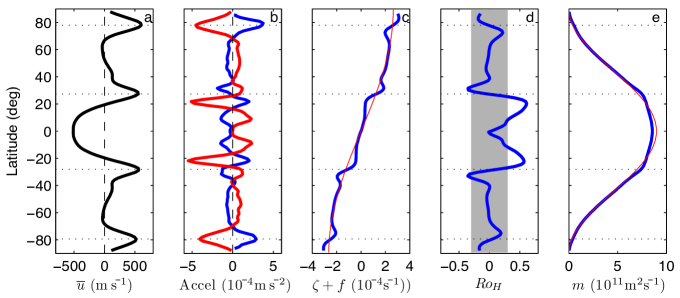
Figure 9.— Zonal-mean, time-mean state of model C$\Omega_{\rm fast}$at 240 mbar. (a) Zonal-mean zonal wind. (b) Total zonal eddy acceleration (sum of last two terms in Equation 9) (blue) and Coriolis acceleration $f\overline{v}$ (red). The strong anticorrelation between these quantities indicates a good balance between them, especially poleward of $30^{\circ}$ latitude. (c) Zonal-mean absolute vorticity, $\overline{\zeta}+f$ (blue) and the Coriolis parameter $f$ itself (red). (d) The Rossby number $Ro_{H}=-\overline{\zeta}/f$. Grey strip corresponds to Rossby numbers with magnitudes less than 0.3, indicating that advection is small relative to the Coriolis acceleration. (e) Zonal-mean angular momentum per unit mass with respect to the planetary rotation axis, $m$ (blue) and the angular momentum of solid-body rotation, $m_{\rm solid}=\Omega a^{2}\cos^{2}\phi$ (red).

Our models show that, in steady state, the zonal eddy acceleration is approximately balanced (away from the equator) by the zonal Coriolis acceleration associated with this mean-meridional circulation. This is demonstrated in Figure 8d, which shows the time-mean $f\overline{v}$ for model C$\Omega_{\rm fast}$. It can be seen that, in most regions, the Coriolis acceleration exhibits a strong anticorrelation with the total eddy acceleration shown in Figure 8c, indicating an approximate balance between the two. This balance is also evident in Figure 9b, which shows the total zonal eddy acceleration (blue) and Coriolis acceleration (red) versus latitude at 200 mbar in model C$\Omega_{\rm fast}$.

To understand this behavior, we can, in a statistical steady state, rewrite the zonal momentum balance (9) as

$$(f+\overline{\zeta})\overline{v}=f(1-Ro_{H})\overline{v}=\overline{\omega}{\partial\overline{u}\over\partial p}+S$$ (10)

where $S$ represents the sum of the two zonal eddy accelerations (the last two terms in Equation 9), $\zeta={\bf k}\cdot\nabla\times{\bf v}$ is the relative vorticity, ${\bf k}$ is the vertical (upward) unit vector, and ${\bf v}$ is the horizontal velocity. In the middle expression, we have defined a Rossby number for the mean-meridional flow, $Ro_{H}=-\overline{\zeta}/f$ (cf Held, 2000; Walker & Schneider, 2006; Schneider & Bordoni, 2008); note that, to order of magnitude, the relative vorticity scales as $\zeta\sim U/L$, where $U$ is a characteristic zonal wind speed and $L$ is a horizontal length scale; thus, $\zeta/f$ essentially equals $Ro\sim U/fL$. Thus, in the rapidly rotating regime, the lefthand side of Equation (10) simplifies to $f\overline{v}$. Likewise, the mean vertical advection term $\overline{\omega}\,\partial{\overline{u}}/\partial p$ can be expressed to order-of-magnitude as $\overline{\omega}\,\overline{u}/\Delta p$, where $\Delta p$ is the pressure thickness of the circulation; the zonal-mean continuity equation implies that $\overline{\omega}/\Delta p\sim\overline{v}/L$, and thus this term is also $Ro$ smaller than $f\overline{v}$. Thus, when the Rossby number is small, Equation (10) leads to the balance

$$f\overline{v}\approx S.$$ (11)

This balance implies that the strength of the mean-meridional circulation in the extratropics is controlled by the eddy-momentum convergence; large eddy momentum convergence leads to a strong meridional circulation and vice versa. Figure 9b shows that, poleward of $\sim$$30^{\circ}$ latitude, the balance (11) is quite good. Over this latitude range, the deviations of the zonal-mean absolute vorticity $\overline{\zeta}+f$ from $f$ itself are generally small (Figure 9c); in agreement, the corresponding extratropical Rossby number $Ro_{H}$ is almost everywhere less than $\sim$0.2 (Figure 9d).

The dynamics of this rapidly rotating regime can be understood by considering the angular momentum per unit mass about the planetary rotation axis, $m=(\Omega a\cos\phi+u)a\cos\phi$. Under small Rossby number, the second term is small compared to the first, which means that dynamics provides only minor perturbations to the planetary (solid-body) contribution. In this case, contours of constant angular momentum are parallel to the rotation axis (essentially vertical in the context of a thin, hydrostatic atmosphere). In this regime, any mean-meridional circulation must cross angular-momentum contours. This can only happen in the presence of eddy-momentum convergences that alter the zonal-mean angular momentum of the air as it moves meridionally. Figure 8f shows contours of $m$ in white, and it can be seen that poleward of $30^{\circ}$, the meridional circulation indeed strongly crosses the angular-momentum contours, and that the $m$-contours are almost vertical, as expected.

At low latitudes, in contrast, the dynamics deviate significantly from the rapidly rotating regime described above. Equatorward of $30^{\circ}$, the angular momentum becomes more slowly varying with latitude (Figure 8f and 9e). This behavior indicates that eddy-momentum convergences do not strongly alter the angular momentum of air as it flows meridionally (at least in comparison to the situation at higher latitudes), so that the meridional circulation is closer to the limit where the angular momentum is conserved following the flow (cf Held & Hou, 1980). Consistent with this picture, the Rossby number $Ro_{H}$ reaches values as high as 0.6 near $20^{\circ}$ latitude (Figure 9c), indicating that—unlike the situation poleward of $30^{\circ}$—meridional momentum advection plays an important role in the zonal momentum budget. This low-latitude regime is analogous to that of Earth’s Hadley circulation, particular the summer cell (e.g., Held & Hou 1980, Walker & Schneider 2006, Schneider & Bordoni 2008; see review in Showman et al. 2013b) and suggests that thermal driving may be an equal or more important factor in controlling the amplitude of this cell than the amplitude of the eddy-momentum convergences. Indeed, it can be seen that, like Earth’s Hadley circulation, the cell extending from $\sim$15–$30^{\circ}$ in each hemisphere is thermally direct, with ascent on the equatorward flank and descent on the poleward flank (Figure 8f).

The relative location of the zonal jets, eddy-momentum convergences, and meridional circulation cells suggests the following picture for the circulation. At high latitudes, the zonal winds are eddy driven. The eastward jet at $\sim$$80^{\circ}$ latitude occurs at precisely the same latitude as the prograde eddy-momentum convergences, which extend coherently—as does the jet—from the top of the model to pressures of $\sim$1 bar (compare Figure 9a and b, or Figure 8a and f). Equation (11) then implies that the jet is co-located with a Ferrel cell, in which air flows equatoward across the jet at pressures $\lesssim 1\rm\,bar$ (Figure 8f). Likewise, the local minimum in zonal wind from $\sim$50–$70^{\circ}$ latitude corresponds well to a broad region of westward eddy acceleration and poleward mean-meridional circulation. This is precisely the picture that has been suggested for the off-equatorial zonal jets on Jupiter and Saturn near cloud level (Showman, 2007; Del Genio et al., 2007; Del Genio & Barbara, 2012; Lian & Showman, 2008; Schneider & Liu, 2009), and would plausibly result from the generation of Rossby waves near the core of the eastward jet and their equatorward propagation into the zonal-flow minimum, where they would break and/or become absorbed at their critical levels (e.g. Dritschel & McIntyre, 2008).

On the other hand, the eastward jet at $\sim$$30^{\circ}$ latitude is more complex. Over much of its vertical extent (from $\sim$0.2–100 mbar), the eddy acceleration is eastward on the jet’s poleward flank but westward on its equatorward flank. Conversely, the Coriolis acceleration (associated with the mean meridional circulation) is westward on the jet’s poleward flank and eastward on its equatorward flank. In the streamfunction (Figure 8f), it is clear that, at $p\lesssim 0.1\,$bar, the jet’s poleward flank corresponds to a Ferrel cell whereas its equatorward flank corresponds to the Hadley cell, with a transition latitude close to the jet axis. This suggests that the jet is a hybrid, corresponding to an eddy-driven jet on its poleward flank and a subtropical jet—i.e., a jet at the poleward edge of a Hadley circulation that is driven by the Coriolis acceleration in the poleward flowing air—on its equatorward flank. Interestingly, the midlatitude local maximum of zonal-mean zonal wind in Earth’s troposphere corresponds to just such a hybrid.

The transition from Hadley to Ferrel cell that occurs near the axis of the $30^{\circ}$-latitude jet suggests that the latitude of this jet—and therefore the width of the the constant-angular-momentum region—is controlled by the location where the jet first becomes baroclinically unstable. Just such a criterion has been proposed as a controlling factor in the width of the Hadley circulation on Earth (e.g. Held, 2000; Lu et al., 2007; Frierson et al., 2007). In the context of a simple two-layer model of a background flow that conserves angular momentum in its upper branch, the lowest latitude of instability is (Held, 2000)

$$\phi_{H}\approx\left({gD\Delta\theta_{v}\over\Omega^{2}a^{2}\theta_{0}}\right)^{1/4}$$ (12)

where $D$ is the layer thickness and $\Delta\theta_{v}/\theta_{0}$ is the fractional variation in potential temperature occurring vertically across the circulation. Inserting the radius and gravity of HD 189733b, $\Omega_{\rm fast}=1.3\times 10^{-4}\rm\,s^{-1}$, $D\approx 300\rm\,km$ appropriate to the multi-scale-height deep circulation in C$\Omega_{\rm fast}$, and $\Delta\theta_{v}/\theta_{0}\approx 1$ yields $\phi_{H}\approx 30^{\circ}$. The agreement with the jet latitude in the simulation is encouraging, though we caution that the two-layer model is crude and its applicability to a continuously stratified, compressible atmosphere extending over many scale heights is perhaps open to question. Nevertheless, the hypothesis is worth testing further in future work.

Our most rapidly rotating, weakly illuminated model, C$\Omega_{\rm fast}$, illuminates the dynamical continuum from hot EGPs to Jupiter and Saturn themselves. Numerous one-layer turbulence studies have suggested that, in rapidly rotating, turbulent, geostrophic flows, the existence of zonal jets is controlled by Rhines scaling, with a meridional jet spacing $L\sim\pi(U/\beta)^{1/2}$ and approximately $N_{\rm jet}\sim a(\beta/U)^{1/2}$ zonal jets from pole to pole, where $U$ is the jet speed (for a review, see Vasavada & Showman, 2005). Inserting $U=600\rm\,m\,s^{-1}$ and $\beta=1.6\times 10^{-12}\rm\,m^{-1}\,s^{-1}$ (appropriate to the off-equatorial jets in C$\Omega_{\rm fast}$) yields $L\approx 60,000\rm\,km$ and $N_{\rm jet}\approx 4$, in agreement with the existence of four eastward jets in this simulation. Inserting $U\approx 30\rm\,s^{-1}$ appropriate for Jupiter’s midlatitudes yields $N_{\rm jet}\approx 16$, similar to the number of eastward jets on Jupiter. This and other similarities suggests that the dynamical regime of C$\Omega_{\rm fast}$resembles Jupiter in important ways. Presumably, models like C$\Omega_{\rm fast}$but with even weaker stellar irradiation would exhibit weaker wind speeds and therefore more jets, approaching Jupiter even more closely.

5.3. Discussion

The above analysis suggests that the equatorial jet direction is controlled by the relative amplitudes of the equatorial versus extratropical wave driving associated with day-night and equator-pole heating gradients, respectively. The day-night (diurnal) forcing drives equatorial waves that attempt to cause equatorial superrotation (cf Showman & Polvani, 2011). In contrast, any baroclinic instabilities induced by the equator-to-pole forcing (i.e., the meridional gradient in zonal-mean heating) induce Rossby waves that propagate meridionally; these waves can become absorbed at critical layers on the equatorward flanks of the off-equatorial subtropical jets, causing a westward acceleration in the equatorial region (Randel & Held, 1991). The net equatorial jet direction depends on which effect dominates. In our models W$\Omega_{\rm slow}$, H$\Omega_{\rm med}$, and H$\Omega_{\rm slow}$, the former effect is far stronger, and the equatorial jet is fast and eastward. On the other hand, in C$\Omega_{\rm fast}$  and W$\Omega_{\rm fast}$, the latter is stronger, leading to (weak) westward flow at the equator. The amplitudes of both wave sources change gradually with rotation rate and incident stellar flux, leading to the transitional behavior described in Section 4 for models C$\Omega_{\rm med}$, W$\Omega_{\rm med}$, and H$\Omega_{\rm fast}$.

This control of equatorial jet direction by equatorial versus mid-latitude wave driving is dynamically similar to that observed in idealized GCMs of Earth and solar-system giant planets that independently vary a zonally symmetric equator-pole forcing and an imposed tropical forcing associated with zonally varying tropical heating anomalies or tropical convection (Suarez & Duffy, 1992; Saravanan, 1993; Kraucunas & Hartmann, 2005; Liu & Schneider, 2010, 2011). In these models, equatorial superrotation occurs when the tropical wave forcing dominates over the mid-latitude wave forcing, while equatorial subrotation (i.e., westward flow) occurs in the reverse case.

These ideas explain the absence of strong superrotation on C$\Omega_{\rm fast}$  despite its existence on Jupiter and Saturn. Models of Jupiter and Saturn have consistently shown that strong convection is a crucial ingredient in causing their equatorial superrotation (e.g. Heimpel et al., 2005; Schneider & Liu, 2009; Kaspi et al., 2009; Lian & Showman, 2010). Jupiter is in a regime where the convection is dynamically important because it is driven by a heat flux comparable to the absorbed solar flux. However, our EGP models have absorbed stellar fluxes ranging from hundreds (C series) to $\sim$$10^{4}$ (H series) times greater than the expected internal convected fluxes. This suggests that internal convection is dynamically unimportant for the photosphere-level atmospheric circulation of warm and hot EGPs. Indeed, our models lack a representation of such convection, implying that when the diurnal forcing is weak, all that remains is the equator-pole forcing, leading to westward equatorial flow as long as rotation is not too slow.

6. Observable implications

Here, we present IR spectra and light curves calculated for our nominal grid of models following the methods described in Fortney et al. (2006), Showman et al. (2008), and Showman et al. (2009). Essentially, given the $T(p)$ profile at each vertical column of the model’s 3D grid, we calculate the local emergent flux radiating toward Earth from that patch of surface. We then sum all such contributions from every surface patch visible from Earth at a given point in the planet’s orbit to obtain an integrated, planet-averaged, wavelength-dependent flux as received at Earth versus orbital phase. Note that this approach naturally accounts for any limb darkening or brightening (associated with longer path lengths through the atmosphere in regions near the planetary limb as viewed from Earth). To compare with previous observed and synthetic light curves (e.g. Showman et al., 2009; Lewis et al., 2010; Kataria et al., 2013, 2014a), we calculate light curves in the Spitzer and WFC3 bandpasses, integrating the emergent flux appropriately over each wavelength-dependent instrument bandpass. To ensure self-consistency, the spectra and lightcurves are calculated using the same radiative transfer model and opacities used in the SPARC model itself. Nevertheless, we use a greater resolution of 196 spectral bins so that spectral features may be better represented.

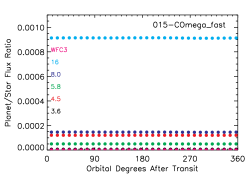
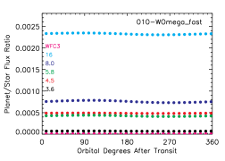
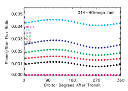
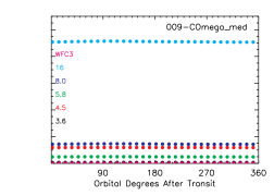
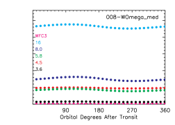
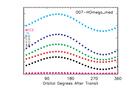
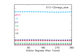
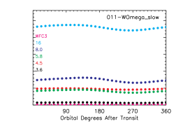
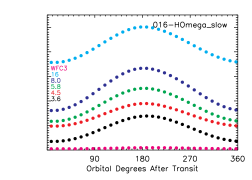
Figure 10.— Light curves in Spitzer IRAC and HST WFC3 bandpasses for the nine runs in the nominal grid. Each panel plots planet-star flux ratio versus orbital phase relative to transit. The left, middle, and right columns adopt rotation periods of 0.55, 2.2, and 8.8 days, respectively. The top, middle, and bottom rows adopt orbital semimajor axes of 0.2, 0.08, and 0.03 AU, respectively.

The resulting light curves are shown in Figure 10. Our cool models exhibit relatively flat light curves, a result of the minimal hemispheric-scale longitudinal temperature differences in these models. In constrast, phase variations are larger in the warm and hot models, a result of the larger longitudinal temperature variations there. For a given incident stellar flux, slowly rotating models exhibit larger phase variations than rapidly rotating models. In the W series, for example, the variations are $\lesssim 5$–10% in the rapidly rotating model but reach 10–20% for the slowly rotating model. Unsurprisingly, the hot models exhibit the largest phase variations, reaching or exceeding a factor-of-two variation at many wavelengths in H$\Omega_{\rm slow}$. In most of the models with prominent phase variations—including all three W models, H$\Omega_{\rm fast}$, and H$\Omega_{\rm med}$—the IR flux peaks precede secondary eclipse, with offets of $\sim$40–$80^{\circ}$. This is the result of advection from the equatorial superrotation (and, in fast rotation cases, the rotation itself) displacing the hot regions to the east. Interestingly, the phase offset is nearly zero in H$\Omega_{\rm slow}$. This results from the fact that, in a synchronously rotating reference frame, the planetary motion is from east-to-west, while the equatorial jet flows from west-to-east; these phenomena lead to rather weak net flow at low latitudes in the synchronously rotating frame, and thus a small offset.

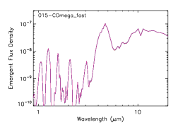
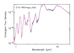
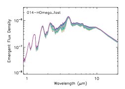
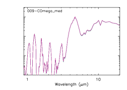
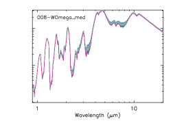
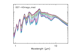
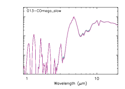
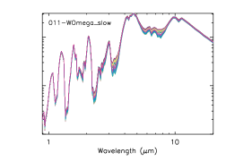
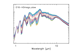
Figure 11.— Infrared spectra for the nine runs in the nominal grid. Different curves show spectra at different orbital phases; this quantifies how the amplitude of phase variations depends on wavelength. The left, middle, and right columns adopt rotation periods of 0.55, 2.2, and 8.8 days, respectively. The top, middle, and bottom rows adopt orbital semimajor axes of 0.2, 0.08, and 0.03 AU, respectively.

Figure 11 shows IR spectra for these same nine models at many different orbital phases. The spectra deviate strongly from a blackbody, especially in the W and C models. Spectral peaks, which represent atmospheric opacity windows, sample deeper pressures where temperatures are high; spectral valleys represent absorption bands that probe lower-pressure, cooler regions. Because the day-night temperature differences tend to increase with decreasing pressure, spectral windows tend to exhibit smaller phase variations than spectral absorption bands. This trend can be prominently seen in Figure 11 where the spread between curves—when it occurs at all—is greatest in the spectral valleys. The C models exhibit essentially no phase variations at any wavelength, except for slight variations near 3.3–$3.5\,\mu$m and 6–$8\,\mu$m in C$\Omega_{\rm slow}$. In the W series, spectral peaks exhibit little phase variation, whereas spectral valleys start to exhibit significant phase variations, reaching a factor of two at $\sim$$2.2\,\mu$m and $3.3\,\mu$m in W$\Omega_{\rm med}$and W$\Omega_{\rm slow}$. Consistent with Figure 10, the spectral phase variations are strongest for the hottest models, and also exhibit significant dependence on rotation rate. Model H$\Omega_{\rm fast}$exhibits peak phase variations of a factor of two from $\sim$2–$3.5\,\mu$m, with little phase variations at many other wavelengths. In contrast, the variations reach a factor of 5–8 at these same wavelengths in H$\Omega_{\rm med}$and H$\Omega_{\rm slow}$.

These light curves and spectra indicate that sufficiently strong non-synchronous rotation can cause observable variations in flux, providing a potential observational test of rotation state. Nevertheless, in practice this may be challenging. For example, the amplitude of the phase variations in H$\Omega_{\rm slow}$  is only a factor of $\sim$2 larger than in H$\Omega_{\rm fast}$, despite the 16-fold difference in rotation rate between these models. Given that atmospheric metallicity, the possible influence of clouds or hazes, and other effects could exert an equal or greater effect on the phase-curve amplitude and offsets, extracting robust information about rotation rate from observational phase variations may be difficult. Our feeling is that order-of-magnitude variations in rotation rate are observationally distinguishable in lightcurves, but that factor of two (or smaller) variations in rotation rate may be degenerate with other unknowns. The real, but modest, effect of rotation in that case would simply be difficult to disentangle from other competing, but poorly constrained, influences on the light curves.

There are several other observational signatures that may help to constrain the dynamics of these warm-to-hot EGPs, including the regime transition discussed here. First, ingress/egress mapping during secondary eclipse could be used to determine the two-dimensional thermal pattern across the dayside (Majeau et al., 2012; de Wit et al., 2012), which may allow observational discrimination between planets with dayside hot spots (like our models H$\Omega_{\rm med}$, H$\Omega_{\rm slow}$, and W$\Omega_{\rm slow}$) versus those with nearly homogeneous temperatures in longitude (like our models C$\Omega_{\rm fast}$, C$\Omega_{\rm med}$, and C$\Omega_{\rm slow}$). Because this technique allows mapping in both longitude and latitude, it may allow latitudinal temperature contrasts to be determined. Second, vertical mixing will likely cause chemical disequilibrium between CO and CH₄ (Cooper & Showman, 2006), and between N₂ and NH₃ for cooler EGPs. Thus photometry and spectra that help to infer the abundances of these species will allow constraints to be placed on the vertical mixing rates. Third, cloud formation would also be expected, particularly in our cooler models and on the nightsides of our warmer models. The longitudinal distribution of cloudiness—which could be constrained via visible-wavelength light curves—likewise will shed light on the circulation regime.

7. Discussion

We presented a systematic analysis of how the atmospheric circulation regime on warm and hot Jupiters varies with incident stellar flux and planetary rotation rate. Basic theoretical arguments suggest that the “canonical” hot Jupiter regime—of large day-night temperature difference and a fast, eastward jet with peak zonal-mean zonal winds at the equator—should give way at smaller stellar flux and/or faster rotation rate to a regime with small longitudinal temperature variations and peak wind speeds occurring in zonal jets at mid-to-high latitudes. We argued on theoretical grounds that the former regime should occur when the radiative time constant at the photosphere is shorter than the solar day whereas the latter should obtain when the radiative time constant is longer than the solar day. To test these ideas and provide a deeper understanding of the dynamical behavior, we performed 3D numerical simulations of the atmospheric flow using the SPARC/MITgcm model, varying the rotation rate over a factor of 16 and the incident stellar flux over a factor of 40.

In agreement with the predictions, our models show that the dynamics exhibits a regime transition from a circulation dominated by an equatorial superrotating jet at high irradiation and slow rotation rates to a regime consisting of off-equatorial eastward jets, with weaker eastward or even westward flow at the equator, at lower irradiation and faster rotation rates. In the latter regime, models at modest-to-slow rotation rate exhibit one eastward jet in each hemisphere, but our fastest-rotating models exhibit multiple eastward jets in each hemisphere and illuminate the dynamical continuum from hot Jupiters to Jupiter and Saturn themselves.

Nevertheless, the apparent simplicity of this transition belies a rich range of dynamical behavior within each regime and associated with their transition. For example, the Rossby number ranges from $\sim$0.1 in the rapidly rotating models to $\gtrsim 1$ in the slowly rotating models, implying that the relative roles of Coriolis forces to momentum advection, the way that eddies act to maintain a mean flow, and the nature of the meridional heat transport undergo significant variation across our ensemble. Several sub-regimes involving significant transitions in the dynamics may may exist within each of the broader regimes emphasized here.

Synthetic light curves and spectra calculated from our models demonstrate that incident stellar flux and planetary rotation rate exert a strong influence on planetary emission. Variations of emission with orbital phase are weak when the incident stellar flux is low, but become significant as the stellar flux increases. At a given stellar flux, slower rotation tends to cause larger-amplitude phase variations, though the effect is modest (order-of-magnitude variations in rotation rate lead to $\sim$factor-of-two changes in phase amplitude). These results indicate that non-synchronous rotation could be inferred from light curves of hot Jupiters if the deviation from synchronous rotation is sufficiently large ($\gtrsim$ factor of two). This is consistent with Showman et al. (2009) and Rauscher & Kempton (2014) and extends their results to a wider range of conditions.

As emphasized by Showman et al. (2009) and Kataria et al. (2014a), the amplitude of phase variations depends significantly on wavelength. The greatest phase variations tend to occur in spectral absorption bands (which probe low-pressure regions that tend to exhibit large day-night temperature differences) and smaller phase variations occur in spectral windows (which probe higher-presssure regions that generally exhibit smaller day-night temperature variations). This wavelength-dependent phase variation becomes significant in our hot and warm models. This signature provides a potentially important way to observationally determine how the day-night temperature difference of a hot Jupiter depends on pressure.

The models presented here pose numerous questions amenable to future research. The regime of weak longitudinal temperature variations and fast mid-to-high latitude jets occurring when $\tau_{\rm rad}>P_{\rm solar}$ has been little explored in the hot-Jupiter literature, but this regime likely dominates the dynamical behavior of EGPs from orbital distances of $\sim$0.1 AU out to several AU. Given that the population of such planets greatly exceeds that of hot Jupiters themselves, further work to understand this regime would be beneficial. For example, most work done in the terrestrial literature on baroclinic instabilities is for the Earth-like application of an atmosphere resting on a surface with a strong entropy gradient, a property that strongly affects the instability. In contrast, it would be useful to explore how baroclinic instabilities equilibrate with the mean flow in the case of a gas giant where a lower impermeable surface plays no role—an area where little work has been done. The extent to which Venus or Titan can provide analogues to the regime of slowly rotating, weakly irradiated EGPs would also be worth investigating. The relative roles of equator-pole and day-night forcing could be disentangled by performing idealized models that vary their ratio. Moreover, additional work is needed—both in the hot Jupiter and more weakly irradiated regime—in the mechanisms controlling the meridional (equator-pole) heat transport, and how that transport depends on parameters. Coupled with improved observations over the coming decade, such an effort would greatly improve our understanding of EGP atmospheric circulation over a broad range of conditions.

References

- Adcroft et al. (2004) Adcroft, A., Campin, J.-M., Hill, C., & Marshall, J. 2004, Monthly Weather Review, 132, 2845
- Amundsen et al. (2014) Amundsen, D. S., Baraffe, I., Tremblin, P., Manners, J., Hayek, W., Mayne, N. J., & Acreman, D. M. 2014, A&A, 564, A59
- Arras & Socrates (2010) Arras, P., & Socrates, A. 2010, ApJ, 714, 1
- Charney (1963) Charney, J. G. 1963, Journal of Atmospheric Sciences, 20, 607
- Conrath et al. (1981) Conrath, B. J., Gierasch, P. J., & Nath, N. 1981, Icarus, 48, 256
- Cooper & Showman (2005) Cooper, C. S., & Showman, A. P. 2005, ApJ, 629, L45
- Cooper & Showman (2006) —. 2006, ApJ, 649, 1048
- Cowan et al. (2012) Cowan, N. B., Machalek, P., Croll, B., Shekhtman, L. M., Burrows, A., Deming, D., Greene, T., & Hora, J. L. 2012, ApJ, 747, 82
- Crossfield et al. (2010) Crossfield, I. J. M., Hansen, B. M. S., Harrington, J., Cho, J., Deming, D., Menou, K., & Seager, S. 2010, ApJ, 723, 1436
- de Wit et al. (2012) de Wit, J., Gillon, M., Demory, B.-O., & Seager, S. 2012, A&A, 548, A128
- Del Genio & Barbara (2012) Del Genio, A. D., & Barbara, J. M. 2012, Icarus, 219, 689
- Del Genio et al. (2007) Del Genio, A. D., Barbara, J. M., Ferrier, J., Ingersoll, A. P., West, R. A., Vasavada, A. R., Spitale, J., & Porco, C. C. 2007, Icarus, 189, 479
- Del Genio & Suozzo (1987) Del Genio, A. D., & Suozzo, R. J. 1987, Journal of Atmospheric Sciences, 44, 973
- Del Genio & Zhou (1996) Del Genio, A. D., & Zhou, W. 1996, Icarus, 120, 332
- Dobbs-Dixon & Agol (2013) Dobbs-Dixon, I., & Agol, E. 2013, MNRAS, 435, 3159
- Dobbs-Dixon & Lin (2008) Dobbs-Dixon, I., & Lin, D. N. C. 2008, ApJ, 673, 513
- Dritschel & McIntyre (2008) Dritschel, D. G., & McIntyre, M. E. 2008, Journal of Atmospheric Sciences, 65, 855
- Fortney et al. (2006) Fortney, J. J., Cooper, C. S., Showman, A. P., Marley, M. S., & Freedman, R. S. 2006, ApJ, 652, 746
- Fortney et al. (2007) Fortney, J. J., Marley, M. S., & Barnes, J. W. 2007, ApJ, 659, 1661
- Frierson et al. (2007) Frierson, D. M. W., Lu, J., & Chen, G. 2007, Geophys. Res. Lett., 34, L18804
- Guillot et al. (1996) Guillot, T., Burrows, A., Hubbard, W. B., Lunine, J. I., & Saumon, D. 1996, ApJ, 459, L35
- Guillot & Showman (2002) Guillot, T., & Showman, A. P. 2002, A&A, 385, 156
- Hartmann (2007) Hartmann, D. L. 2007, J. Meteor. Soc. Japan, 85B, 123
- Heimpel et al. (2005) Heimpel, M., Aurnou, J., & Wicht, J. 2005, Nature, 438, 193
- Held (1975) Held, I. M. 1975, Journal of the Atmospheric Sciences, 32, 1494
- Held (2000) —. 2000, Paper presented at 2000 Woods Hole Oceanographic Institute Geophysical Fluid Dynamics Program, Woods Hole Oceanographic Institute, Woods Hole, MA (available at http://www.whoi.edu/page.do?pid=13076)
- Held & Andrews (1983) Held, I. M., & Andrews, D. G. 1983, Journal of Atmospheric Sciences, 40, 2220
- Held & Hou (1980) Held, I. M., & Hou, A. Y. 1980, Journal of Atmospheric Sciences, 37, 515
- Heng et al. (2011a) Heng, K., Frierson, D. M. W., & Phillipps, P. J. 2011a, MNRAS, 418, 2669
- Heng et al. (2011b) Heng, K., Menou, K., & Phillipps, P. J. 2011b, MNRAS, 413, 2380
- Holton (2004) Holton, J. R. 2004, An Introduction to Dynamic Meteorology, 4th Ed. (Academic Press, San Diego)
- James (1987) James, I. N. 1987, Journal of Atmospheric Sciences, 44, 3710
- Karoly et al. (1998) Karoly, D. J., Vincent, D. G., & Shrage, J. M. 1998, General circulation. In Meteorology of the Southern Hemisphere, American Meteorological Society Monographs, vol. 27 (American Meterological Society), 47–85
- Kaspi et al. (2009) Kaspi, Y., Flierl, G. R., & Showman, A. P. 2009, Icarus, 202, 525
- Kaspi & Showman (2014) Kaspi, Y., & Showman, A. 2014, ArXiv e-prints
- Kataria et al. (2014a) Kataria, T., Showman, A. P., Fortney, J. J., Marley, M. S., & Freedman, R. S. 2014a, ApJ, 785, 92
- Kataria et al. (2014b) Kataria, T., Showman, A. P., Fortney, J. J., Stevenson, K. B., Line, M. R., Kreidberg, L., Bean, J. L., & Désert, J.-M. 2014b, ArXiv e-prints
- Kataria et al. (2013) Kataria, T., Showman, A. P., Lewis, N. K., Fortney, J. J., Marley, M. S., & Freedman, R. S. 2013, ApJ, 767, 76
- Kirk & Stevenson (1987) Kirk, R. L., & Stevenson, D. J. 1987, ApJ, 316, 836
- Knutson et al. (2012) Knutson, H. A., Lewis, N., Fortney, J. J., Burrows, A., Showman, A. P., Cowan, N. B., Agol, E., Aigrain, S., Charbonneau, D., Deming, D., Désert, J.-M., Henry, G. W., Langton, J., & Laughlin, G. 2012, ApJ, 754, 22
- Kraucunas & Hartmann (2005) Kraucunas, I., & Hartmann, D. L. 2005, J. Atmos. Sci., 62, 371
- Lewis et al. (2013) Lewis, N. K., Knutson, H. A., Showman, A. P., Cowan, N. B., Laughlin, G., Burrows, A., Deming, D., Crepp, J. R., Mighell, K. J., Agol, E., Bakos, G. Á., Charbonneau, D., Désert, J.-M., Fischer, D. A., Fortney, J. J., Hartman, J. D., Hinkley, S., Howard, A. W., Johnson, J. A., Kao, M., Langton, J., & Marcy, G. W. 2013, ApJ, 766, 95
- Lewis et al. (2014) Lewis, N. K., Showman, A. P., Fortney, J. J., Knutson, H. A., & Marley, M. S. 2014, ArXiv e-prints
- Lewis et al. (2010) Lewis, N. K., Showman, A. P., Fortney, J. J., Marley, M. S., Freedman, R. S., & Lodders, K. 2010, ApJ, 720, 344
- Li & Goodman (2010) Li, J., & Goodman, J. 2010, ApJ, 725, 1146
- Lian & Showman (2008) Lian, Y., & Showman, A. P. 2008, Icarus, 194, 597
- Lian & Showman (2010) —. 2010, Icarus, 207, 373
- Lindzen (1981) Lindzen, R. S. 1981, J. Geophys. Res., 86, 9707
- Liu & Showman (2013) Liu, B., & Showman, A. P. 2013, ApJ, 770, 42
- Liu et al. (2008) Liu, J., Goldreich, P. M., & Stevenson, D. J. 2008, Icarus, 196, 653
- Liu & Schneider (2010) Liu, J., & Schneider, T. 2010, Journal of Atmospheric Sciences, 67, 3652
- Liu & Schneider (2011) —. 2011, Journal of Atmospheric Sciences, 68, 2742
- Lu et al. (2007) Lu, J., Vecchi, G. A., & Reichler, T. 2007, Geophys. Res. Lett., 34 (L06805)
- Majeau et al. (2012) Majeau, C., Agol, E., & Cowan, N. B. 2012, ApJ, 747, L20
- Marley & McKay (1999) Marley, M. S., & McKay, C. P. 1999, Icarus, 138, 268
- Mayne et al. (2014) Mayne, N. J., Baraffe, I., Acreman, D. M., Smith, C., Browning, M. K., Skålid Amundsen, D., Wood, N., Thuburn, J., & Jackson, D. R. 2014, A&A, 561, A1
- Menou & Rauscher (2009) Menou, K., & Rauscher, E. 2009, ApJ, 700, 887
- Menou & Rauscher (2010) —. 2010, ApJ, 713, 1174
- Mitchell et al. (2006) Mitchell, J. L., Pierrehumbert, R. T., Frierson, D. M. W., & Caballero, R. 2006, Proceedings of the National Academy of Science, 103, 18421
- Mitchell & Vallis (2010) Mitchell, J. L., & Vallis, G. K. 2010, Journal of Geophysical Research (Planets), 115, 12008
- O’Gorman & Schneider (2008) O’Gorman, P. A., & Schneider, T. 2008, Journal of Atmospheric Sciences, 65, 524
- Panetta (1993) Panetta, R. L. 1993, Journal of Atmospheric Sciences, 50, 2073
- Perez-Becker & Showman (2013) Perez-Becker, D., & Showman, A. P. 2013, ApJ, 776, 134
- Perna et al. (2012) Perna, R., Heng, K., & Pont, F. 2012, ApJ, 751, 59
- Perna et al. (2010) Perna, R., Menou, K., & Rauscher, E. 2010, ApJ, 719, 1421
- Pierrehumbert & Swanson (1995) Pierrehumbert, R. T., & Swanson, K. L. 1995, Annu. Rev. Fluid Mech., 27, 419
- Polichtchouk & Cho (2012) Polichtchouk, I., & Cho, J. Y.-K. 2012, MNRAS, 424, 1307
- Randel & Held (1991) Randel, W. J., & Held, I. M. 1991, Journal of Atmospheric Sciences, 48, 688
- Rasio et al. (1996) Rasio, F. A., Tout, C. A., Lubow, S. H., & Livio, M. 1996, ApJ, 470, 1187
- Rauscher & Kempton (2014) Rauscher, E., & Kempton, E. M. R. 2014, ApJ, 790, 79
- Rauscher & Menou (2010) Rauscher, E., & Menou, K. 2010, ApJ, 714, 1334
- Rauscher & Menou (2012a) —. 2012a, ApJ, 750, 96
- Rauscher & Menou (2012b) —. 2012b, ApJ, 745, 78
- Rauscher & Menou (2013) —. 2013, ApJ, 764, 103
- Read (1988) Read, P. L. 1988, Quarterly Journal of the Royal Meteorological Society, 114, 421
- Rogers & Showman (2014) Rogers, T. M., & Showman, A. P. 2014, ApJ, 782, L4
- Saravanan (1993) Saravanan, R. 1993, J. Atmos. Sci., 50, 1211
- Schneider & Bordoni (2008) Schneider, T., & Bordoni, S. 2008, Journal of Atmospheric Sciences, 65, 915
- Schneider & Liu (2009) Schneider, T., & Liu, J. 2009, J. Atmos. Sci., 66, 579
- Showman (2007) Showman, A. P. 2007, J. Atmos. Sci., 64, 3132
- Showman et al. (2008) Showman, A. P., Cooper, C. S., Fortney, J. J., & Marley, M. S. 2008, ApJ, 682, 559
- Showman et al. (2013a) Showman, A. P., Fortney, J. J., Lewis, N. K., & Shabram, M. 2013a, ApJ, 762, 24
- Showman et al. (2009) Showman, A. P., Fortney, J. J., Lian, Y., Marley, M. S., Freedman, R. S., Knutson, H. A., & Charbonneau, D. 2009, ApJ, 699, 564
- Showman & Guillot (2002) Showman, A. P., & Guillot, T. 2002, A&A, 385, 166
- Showman & Polvani (2010) Showman, A. P., & Polvani, L. M. 2010, Geophys. Res. Lett., 37, 18811
- Showman & Polvani (2011) —. 2011, ApJ, 738, 71
- Showman et al. (2013b) Showman, A. P., Wordsworth, R. D., Merlis, T. M., & Kaspi, Y. 2013b, Atmospheric Circulation of Terrestrial Exoplanets. In Comparative Climatology of Terrestrial Planets (Mackwell, S.J., Simon-Miller, A.A., Harder, J.W., and Bullock, M.A., Eds.) (Univ. Arizona Press), 277–326
- Stevenson et al. (2014) Stevenson, K. B., coauthors, X. X., & morecoauthors, X. X. 2014, Science, submitted
- Suarez & Duffy (1992) Suarez, M. J., & Duffy, D. G. 1992, J. Atmos. Sci., 49, 1541
- Thompson (1971) Thompson, R. O. R. Y. 1971, Journal of Physical Oceanography, 1, 235
- Thrastarson & Cho (2010) Thrastarson, H. T., & Cho, J. 2010, ApJ, 716, 144
- Tsai et al. (2014) Tsai, S.-M., Dobbs-Dixon, I., & Gu, P.-G. 2014, ArXiv e-prints
- Vallis (2006) Vallis, G. K. 2006, Atmospheric and Oceanic Fluid Dynamics: Fundamentals and Large-Scale Circulation (Cambridge Univ. Press, Cambridge, UK)
- Vasavada & Showman (2005) Vasavada, A. R., & Showman, A. P. 2005, Reports of Progress in Physics, 68, 1935
- Walker & Schneider (2006) Walker, C. C., & Schneider, T. 2006, Journal of Atmospheric Sciences, 63, 3333
- Wallace & Hobbs (2004) Wallace, J. M., & Hobbs, P. V. 2004, Atmospheric Science: An Introductory Survey, 2nd Ed. (Academic Press, San Diego)
- Wang (1990) Wang, B. 1990, Tellus A, Vol. 42, issue 4, p.463, 42, 463
- Williams (1979) Williams, G. P. 1979, Journal of Atmospheric Sciences, 36, 932
- Williams (2003) —. 2003, Journal of Atmospheric Sciences, 60, 1270
- Zellem et al. (2014) Zellem, R. T., Lewis, N. K., Knutson, H. A., Griffith, C. A., Showman, A. P., Fortney, J. J., Cowan, N. B., Agol, E., Burrows, A., Charbonneau, D., Deming, D., Laughlin, G., & Langton, J. 2014, ApJ, 790, 53