Quantifying Redundant Information in Predicting a Target Random Variable

Abstract

This paper considers the problem of defining a measure of redundant information that quantifies how much common information two or more random variables specify about a target random variable. We discussed desired properties of such a measure, and propose new measures with some desirable properties.

I Introduction

Many molecular and neurological systems involve multiple interacting factors affecting an outcome synergistically and/or redundantly. Attempts to shed light on issues such as population coding in neurons, or genetic contribution to a phenotype (e.g. eye-color), have motivated various proposals to leverage principled information-theoretic measures for quantifying informational synergy and redundancy, e.g. [1, 2, 3, 4, 5]. In these settings, we are concerned with the statistics of how two (or more) random variables $X_{1},X_{2}$, called predictors, jointly or separately specify/predict another random variable $Y$, called a target random variable. This focus on a target random variable is in contrast to Shannon’s mutual information which quantifies statistical dependence between two random variables, and various notions of common information, e.g. [6, 7, 8].

The concepts of synergy and redundancy are based on several intuitive notions, e.g., positive informational synergy indicates that $X_{1}$ and $X_{2}$ act cooperatively or antagonistically to influence $Y$; positive redundancy indicates there is an aspect of $Y$ that $X_{1}$ and $X_{2}$ can each separately predict. However, it has proven challenging[9, 10, 11, 12] to come up with precise information-theoretic definitions of synergy and redundancy that are consistent with all intuitively desired properties.

II Background: Partial Information Decomposition

The Partial Information Decomposition (PID) approach of [13] defines the concepts of synergistic, redundant and unique information in terms of intersection information, $\operatorname{I}_{\cap}\!\left(\{X_{1},\ldots,X_{n}\}\!\mathrel{\mathop{\mathchar 58\relax}}\!Y\right)$, which quantifies the common information that each of the $n$ predictors $X_{1},\ldots,X_{n}$ conveys about a target random variable $Y$. An antichain lattice of redundant, unique, and synergistic partial informations is built from the intersection information.

Partial information diagrams (PI-diagrams) extend Venn diagrams to represent synergy. A PI-diagram is composed of nonnegative partial information regions (PI-regions). Unlike the standard Venn entropy diagram in which the sum of all regions is the joint entropy $\operatornamewithlimits{H}\!\left(X_{1\ldots n},Y\right)$, in PI-diagrams the sum of all regions (i.e. the space of the PI-diagram) is the mutual information $\operatornamewithlimits{I}\!\left(X_{1\ldots n}\!\mathrel{\mathop{\mathchar 58\relax}}\!Y\right)$. PI-diagrams show how the mutual information $\operatornamewithlimits{I}\!\left(X_{1\ldots n}\!\mathrel{\mathop{\mathchar 58\relax}}\!Y\right)$ is distributed across subsets of the predictors. For example, in the PI-diagram for $n=2$ (Figure 1): $\{1\}$ denotes the unique information about $Y$ that only $X_{1}$ carries (likewise {2} denotes the information only $X_{2}$ carries); $\{1,2\}$ denotes the redundant information about $Y$ that $X_{1}$ as well as $X_{2}$ carries, while $\{12\}$ denotes the information about $Y$ that is specified only by $X_{1}$ and $X_{2}$ synergistically or jointly.

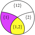
(a) $\operatornamewithlimits{I}\!\left(X_{1}\!\mathrel{\mathop{\mathchar 58\relax}}\!Y\right)$

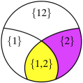
(b) $\operatornamewithlimits{I}\!\left(X_{2}\!\mathrel{\mathop{\mathchar 58\relax}}\!Y\right)$

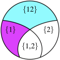
(c) $\operatornamewithlimits{I}\!\left(X_{1}\!\mathrel{\mathop{\mathchar 58\relax}}\!Y|X_{2}\right)$

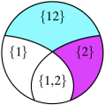
(d) $\operatornamewithlimits{I}\!\left(X_{2}\!\mathrel{\mathop{\mathchar 58\relax}}\!Y|X_{1}\right)$

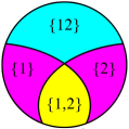
(e) $\operatornamewithlimits{I}\!\left(X_{1}X_{2}\!\mathrel{\mathop{\mathchar 58\relax}}\!Y\right)$

Figure 1: PI-diagrams for $n=2$ predictors, showing the amount of redundant (yellow/bottom), unique (magenta/left and right) and synergistic (cyan/top) information with respect to the target $Y$.

Each PI-region is either redundant, unique, or synergistic, but any combination of positive PI-regions may be possible. Per [13], for two predictors, the four partial informations are defined as follows: the redundant information as $\operatorname{I}_{\cap}\!\left(\{X_{1},X_{2}\}\!\mathrel{\mathop{\mathchar 58\relax}}\!Y\right)$, the unique informations as

$$\begin{split}\operatorname{I}_{\partial}(X_{1}\mathrel{\mathop{\mathchar 58\relax}}Y)&=\operatornamewithlimits{I}\!\left(X_{1}\!\mathrel{\mathop{\mathchar 58\relax}}\!Y\right)-\operatorname{I}_{\cap}\!\left(\{X_{1},X_{2}\}\!\mathrel{\mathop{\mathchar 58\relax}}\!Y\right)\\ \operatorname{I}_{\partial}(X_{2}\mathrel{\mathop{\mathchar 58\relax}}Y)&=\operatornamewithlimits{I}\!\left(X_{2}\!\mathrel{\mathop{\mathchar 58\relax}}\!Y\right)-\operatorname{I}_{\cap}\!\left(\{X_{1},X_{2}\}\!\mathrel{\mathop{\mathchar 58\relax}}\!Y\right),\end{split}$$ (1)

and the synergistic information as

$$\begin{split}&\operatorname{I}_{\partial}(X_{1},X_{2}\mathrel{\mathop{\mathchar 58\relax}}Y)\\ &=\operatornamewithlimits{I}\!\left(X_{1},X_{2}\!\mathrel{\mathop{\mathchar 58\relax}}\!Y\right)-\operatorname{I}_{\partial}\left(X_{1}\mathrel{\mathop{\mathchar 58\relax}}Y\right)-\operatorname{I}_{\partial}\left(X_{2}\mathrel{\mathop{\mathchar 58\relax}}Y\right)\\ &\hskip 7.22743pt-\operatorname{I}_{\partial}\left(X_{1},X_{2}\mathrel{\mathop{\mathchar 58\relax}}Y\right)\;\\ &=\operatornamewithlimits{I}\!\left(X_{1},X_{2}\!\mathrel{\mathop{\mathchar 58\relax}}\!Y\right)-\operatornamewithlimits{I}\!\left(X_{1}\!\mathrel{\mathop{\mathchar 58\relax}}\!Y\right)-\operatornamewithlimits{I}\!\left(X_{2}\!\mathrel{\mathop{\mathchar 58\relax}}\!Y\right)+\operatorname{I}_{\cap}\!\left(\{X_{1},X_{2}\}\!\mathrel{\mathop{\mathchar 58\relax}}\!Y\right).\end{split}$$ (2)

III Desired $\operatorname{I}_{\cap}$ properties and canonical examples

There are a number of intuitive properties, proposed in [13, 9, 10, 11, 5, 12], that are considered desirable for the intersection information measure $\operatorname{I}_{\cap}$ to satisfy:

• Weak Symmetry: $\operatorname{I}_{\cap}\!\left(\{X_{1},\ldots,X_{n}\}\!\mathrel{\mathop{\mathchar 58\relax}}\!Y\right)$ is invariant under reordering of $X_{1},\ldots,X_{n}$.

• Weak Monotonicity: $\operatorname{I}_{\cap}\!\left(\{X_{1},\ldots,X_{n},Z\}\!\mathrel{\mathop{\mathchar 58\relax}}\!Y\right)\leq\operatorname{I}_{\cap}\!\left(\{X_{1},\ldots,X_{n}\}\!\mathrel{\mathop{\mathchar 58\relax}}\!Y\right)$ with equality if there exists $X_{i}\in\{X_{1},\ldots,X_{n}\}$ such that $\operatornamewithlimits{H}\!\left(Z,X_{i}\right)=\operatornamewithlimits{H}\!\left(Z\right)$.

• Self-Redundancy: $\operatorname{I}_{\cap}\!\left(\{X_{1}\}\!\mathrel{\mathop{\mathchar 58\relax}}\!Y\right)=\operatornamewithlimits{I}\!\left(X_{1}\!\mathrel{\mathop{\mathchar 58\relax}}\!Y\right)$. The intersection information a single predictor $X_{1}$ conveys about the target $Y$ is equal to the mutual information between the $X_{1}$ and the target $Y$.

• Strong Monotonicity: $\operatorname{I}_{\cap}\!\left(\{X_{1},\ldots,X_{n},Z\}\!\mathrel{\mathop{\mathchar 58\relax}}\!Y\right)\leq\operatorname{I}_{\cap}\!\left(\{X_{1},\ldots,X_{n}\}\!\mathrel{\mathop{\mathchar 58\relax}}\!Y\right)$ with equality if there exists $X_{i}\in\{X_{1},\ldots,X_{n}\}$ such that $\operatornamewithlimits{I}\!\left(Z,X_{i}\!\mathrel{\mathop{\mathchar 58\relax}}\!Y\right)=\operatornamewithlimits{I}\!\left(Z\!\mathrel{\mathop{\mathchar 58\relax}}\!Y\right)$.

• Local Positivity: For all $n$, the derived “partial informations” defined in [13] are nonnegative. This is equivalent to requiring that $\operatorname{I}_{\cap}$ satisfy total monotonicity, a stronger form of supermodularity. For $n=2$ this can be concretized as, $\operatorname{I}_{\cap}\!\left(\{X_{1},X_{2}\}\!\mathrel{\mathop{\mathchar 58\relax}}\!Y\right)\geq\operatornamewithlimits{I}\!\left(X_{1}\!\mathrel{\mathop{\mathchar 58\relax}}\!X_{2}\right)-\operatornamewithlimits{I}\!\left(X_{1}\!\mathrel{\mathop{\mathchar 58\relax}}\!X_{2}\middle|Y\right)$.

• Target Monotonicity: If $\operatornamewithlimits{H}\!\left(Y|Z\right)=0$, then $\operatorname{I}_{\cap}\!\left(\{X_{1},\ldots,X_{n}\}\!\mathrel{\mathop{\mathchar 58\relax}}\!Y\right)\leq\operatorname{I}_{\cap}\!\left(\{X_{1},\ldots,X_{n}\}\!\mathrel{\mathop{\mathchar 58\relax}}\!Z\right)$.

There are also a number of canonical examples for which one or more of the partial informations have intuitive values, which are considered desirable for the intersection information measure $\operatorname{I}_{\cap}$ to attain.

Example Unq, shown in Figure 2, is a canonical case of unique information, in which each predictor carries independent information about the target. $Y$ has four equiprobable states: ab, aB, Ab, and AB. $X_{1}$ uniquely specifies bit a/A, and $X_{2}$ uniquely specifies bit b/B. Note that the states are named so as to highlight the two bits of unique information; it is equivalent to choose any four unique names for the four states.

$X_{1}$ $X_{2}$	$Y$
a b	ab	$\nicefrac{{1}}{{4}}$
a B	aB	$\nicefrac{{1}}{{4}}$
A b	Ab	$\nicefrac{{1}}{{4}}$
A B	AB	$\nicefrac{{1}}{{4}}$

(a) $\Pr\!\left(x_{1},x_{2},y\right)$

$$\operatornamewithlimits{I}\!\left(X_{1},X_{2}\!\mathrel{\mathop{\mathchar 58\relax}}\!Y\right) =2$$

$$\operatornamewithlimits{I}\!\left(X_{1}\!\mathrel{\mathop{\mathchar 58\relax}}\!Y\right) =1$$

$$\operatornamewithlimits{I}\!\left(X_{2}\!\mathrel{\mathop{\mathchar 58\relax}}\!Y\right) =1$$

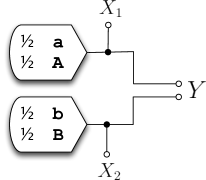
(b) circuit diagram

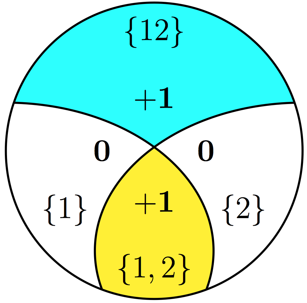
(c) $\operatorname{I}_{\min}$

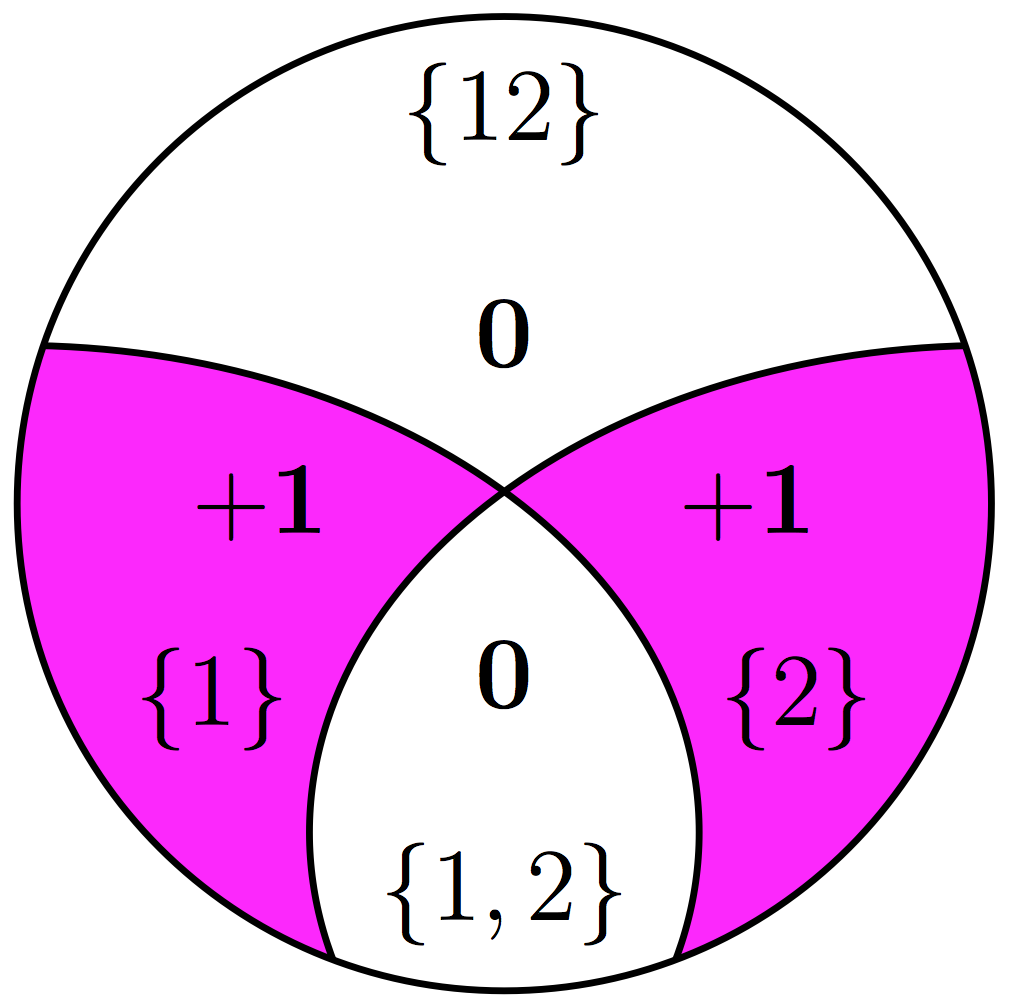
(d) Syn/$\Delta\operatorname{I}$/$\operatorname{I}_{\wedge}$/$\operatorname{I}_{\alpha}$

Figure 2: Example Unq. $X_{1}$ and $X_{2}$ each uniquely carry one bit of information about $Y$. $\operatornamewithlimits{I}\!\left(X_{1}X_{2}\!\mathrel{\mathop{\mathchar 58\relax}}\!Y\right)~{}=~{}\operatornamewithlimits{H}\!\left(Y\right)~{}=~{}2$ bits.

Example RdnXor, shown in Figure 3, is a canonical example of redundancy and synergy coexisting. The r/R bit is redundant, while the 0/1 bit of $Y$ is synergistically specified as the XOR of the corresponding bits in $X_{1}$ and $X_{2}$.

$X_{1}$ $X_{2}$	$Y$
r0 r0	r0	$\nicefrac{{1}}{{8}}$
r0 r1	r1	$\nicefrac{{1}}{{8}}$
r1 r0	r1	$\nicefrac{{1}}{{8}}$
r1 r1	r0	$\nicefrac{{1}}{{8}}$
R0 R0	R0	$\nicefrac{{1}}{{8}}$
R0 R1	R1	$\nicefrac{{1}}{{8}}$
R1 R0	R1	$\nicefrac{{1}}{{8}}$
R1 R1	R0	$\nicefrac{{1}}{{8}}$

(a) $\Pr\!\left(x_{1},x_{2},y\right)$

$$\operatornamewithlimits{I}\!\left(X_{1},X_{2}\!\mathrel{\mathop{\mathchar 58\relax}}\!Y\right) =2$$

$$\operatornamewithlimits{I}\!\left(X_{1}\!\mathrel{\mathop{\mathchar 58\relax}}\!Y\right) =1$$

$$\operatornamewithlimits{I}\!\left(X_{2}\!\mathrel{\mathop{\mathchar 58\relax}}\!Y\right) =1$$

$$\operatorname{I}_{\min}\!\left(\{X_{1},X_{2}\}\!\mathrel{\mathop{\mathchar 58\relax}}\!Y\right) =1$$

$$\operatorname{I}_{\wedge}\!\left(\{X_{1},X_{2}\}\!\mathrel{\mathop{\mathchar 58\relax}}\!Y\right) =1$$

$$\operatorname{I}_{\alpha}\!\left(\{X_{1},X_{2}\}\mathrel{\mathop{\mathchar 58\relax}}Y\right) =1$$

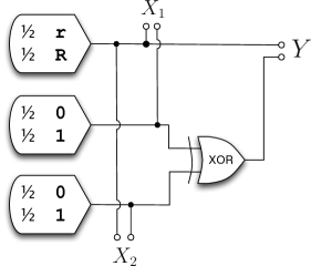
(b) circuit diagram

(c) Syn

(d) $\Delta\operatorname{I}$/$\operatorname{I}_{\min}$/$\operatorname{I}_{\wedge}$/$\operatorname{I}_{\alpha}$

Figure 3: Example RdnXor. This is the canonical example of redundancy and synergy coexisting. $\operatorname{I}_{\min}$ and $\operatorname{I}_{\wedge}$ each reach the desired decomposition of one bit of redundancy and one bit of synergy. This example demonstrates $\operatorname{I}_{\wedge}$ correctly extracting the embedded redundant bit within $X_{1}$ and $X_{2}$.

Example And, shown in Figure 4, is an example where the relationship between $X_{1},X_{2}$ and $Y$ is nonlinear, making the desired partial information values less intuitively obvious. Nevertheless, it is desired that the partial information values should be nonnegative.

$X_{1}$ $X_{2}$	$Y$
0 0	0	$\nicefrac{{1}}{{4}}$
0 1	0	$\nicefrac{{1}}{{4}}$
1 0	0	$\nicefrac{{1}}{{4}}$
1 1	1	$\nicefrac{{1}}{{4}}$

(a) $\Pr\!\left(x_{1},x_{2},y\right)$

$$\operatornamewithlimits{I}\!\left(X_{1},X_{2}\!\mathrel{\mathop{\mathchar 58\relax}}\!Y\right) =0.811$$

$$\operatornamewithlimits{I}\!\left(X_{1}\!\mathrel{\mathop{\mathchar 58\relax}}\!Y\right) =0.311$$

$$\operatornamewithlimits{I}\!\left(X_{2}\!\mathrel{\mathop{\mathchar 58\relax}}\!Y\right) =0.311$$

$$\operatorname{I}_{\min}\!\left(\{X_{1},X_{2}\}\!\mathrel{\mathop{\mathchar 58\relax}}\!Y\right) =0.311$$

$$\operatorname{I}_{\wedge}\!\left(\{X_{1},X_{2}\}\!\mathrel{\mathop{\mathchar 58\relax}}\!Y\right) =0$$

$$\operatorname{I}_{\alpha}\!\left(\{X_{1},X_{2}\}\mathrel{\mathop{\mathchar 58\relax}}Y\right) =0$$

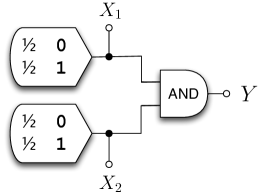
(b) circuit diagram

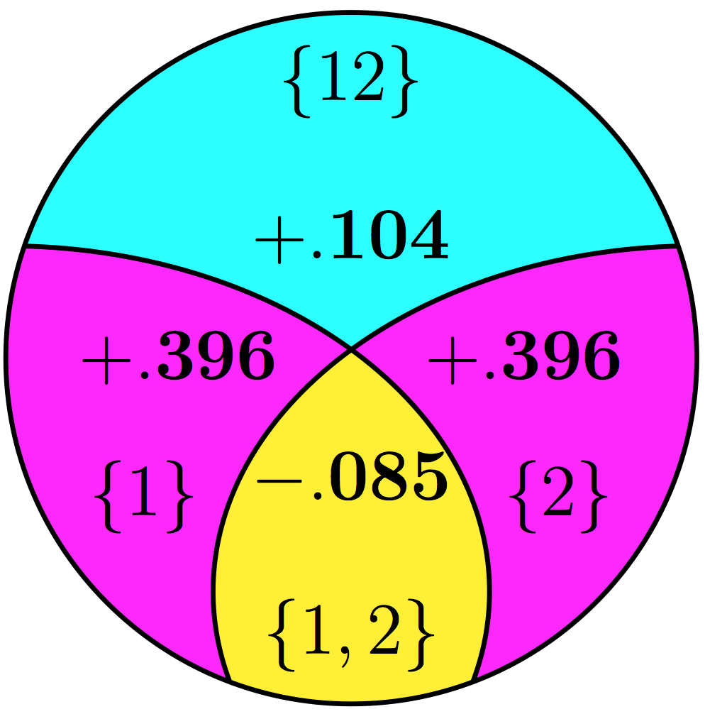
(c) $\Delta\operatorname{I}$

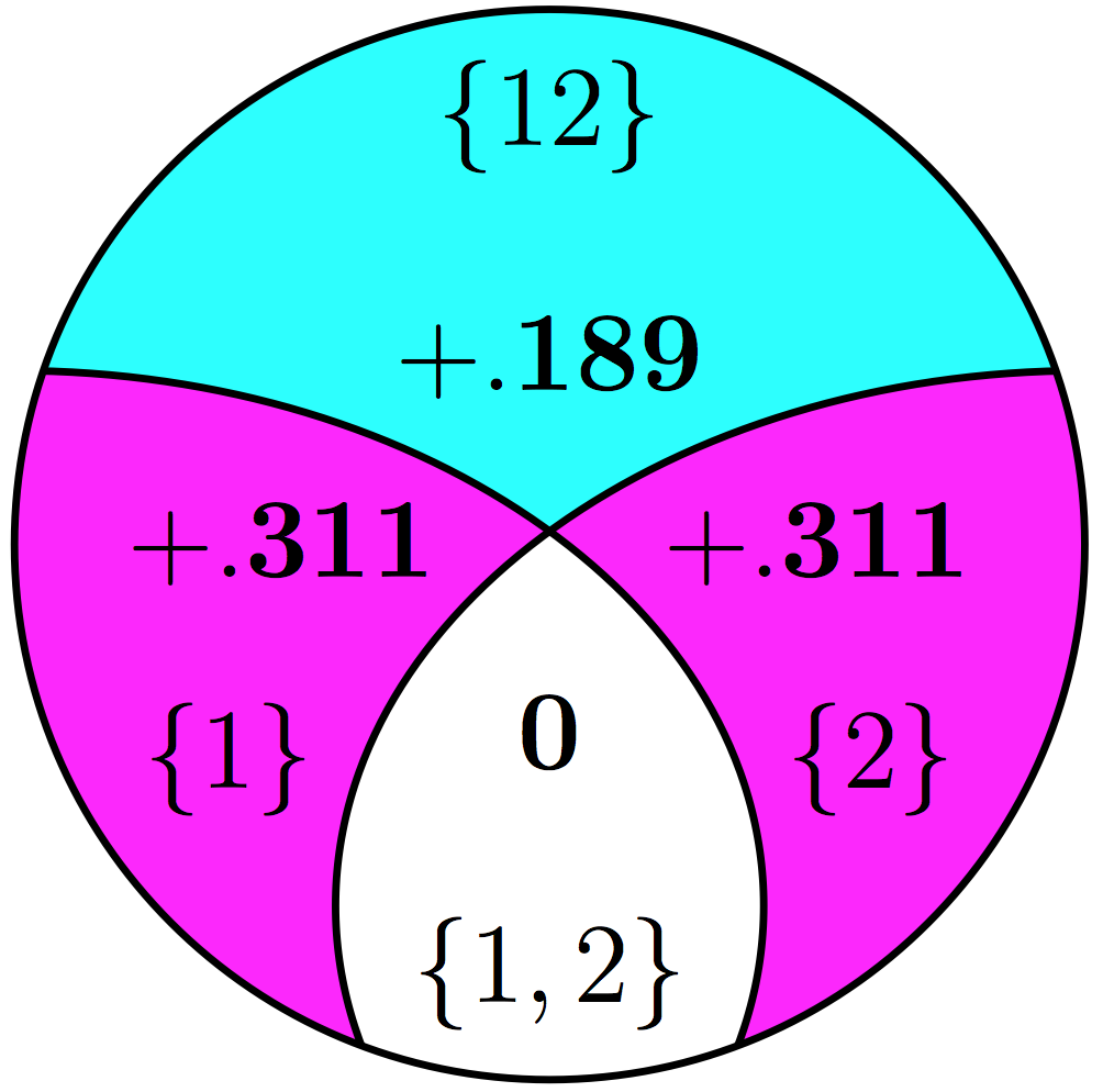
(d) Syn/$\operatorname{I}_{\wedge}$/$\operatorname{I}_{\alpha}$

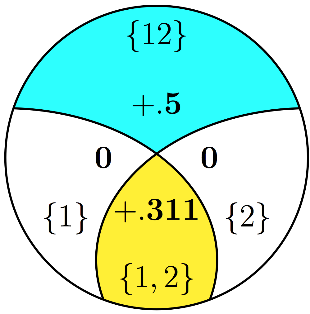
(e) $\operatorname{I}_{\min}$

Figure 4: Example And. $\Delta\operatorname{I}$ yields a redundant information of negative $.085$ bits. There are arguments for the redundant information being zero or positive, but thus far all that is agreed upon is that the redundant information is between $[0,0.311]$ bits.

Example ImperfectRdn, shown in Figure 5, is an example of “imperfect” or “lossy” correlation between the predictors, where it is intuitively desirable that the derived redundancy should be positive. Given $\mathbf{(LP)}$, we can determine the desired decomposition analytically. First, $\operatornamewithlimits{I}\!\left(X_{1},X_{2}\!\mathrel{\mathop{\mathchar 58\relax}}\!Y\right)=\operatornamewithlimits{I}\!\left(X_{1}\!\mathrel{\mathop{\mathchar 58\relax}}\!Y\right)=1$ bit; therefore, $\operatornamewithlimits{I}\!\left(X_{2}\!\mathrel{\mathop{\mathchar 58\relax}}\!Y|X_{1}\right)=\operatornamewithlimits{I}\!\left(X_{1},X_{2}\!\mathrel{\mathop{\mathchar 58\relax}}\!Y\right)-\operatornamewithlimits{I}\!\left(X_{1}\!\mathrel{\mathop{\mathchar 58\relax}}\!Y\right)~{}=~{}0$ bits. This determines two of the partial informations—the synergistic information $\operatorname{I}_{\partial}\!\left(X_{1},X_{2}\!\mathrel{\mathop{\mathchar 58\relax}}\!Y\right)$ and the unique information $\operatorname{I}_{\partial}\!\left(X_{2}\!\mathrel{\mathop{\mathchar 58\relax}}\!Y\right)$ are both zero. Then, the redundant information $\operatorname{I}_{\partial}\!\left(X_{1},X_{2}\!\mathrel{\mathop{\mathchar 58\relax}}\!Y\right)=\operatornamewithlimits{I}\!\left(X_{2}\!\mathrel{\mathop{\mathchar 58\relax}}\!Y\right)-\operatorname{I}_{\partial}(X_{2}\mathrel{\mathop{\mathchar 58\relax}}Y)=\operatornamewithlimits{I}\!\left(X_{2}\!\mathrel{\mathop{\mathchar 58\relax}}\!Y\right)=0.99$ bits. Having determined three of the partial informations, we compute the final unique information $\operatorname{I}_{\partial}\!\left(X_{1}\!\mathrel{\mathop{\mathchar 58\relax}}\!Y\right)=\operatornamewithlimits{I}\!\left(X_{1}\!\mathrel{\mathop{\mathchar 58\relax}}\!Y\right)-0.99=0.01$ bits.

$\ \,X_{1}\,X_{2}$	$Y$
0 0	0	$0.499$
0 1	0	$0.001$
1 1	1	$0.500$

(a) $\Pr\!\left(x_{1},x_{2},y\right)$

$$\operatornamewithlimits{I}\!\left(X_{1},X_{2}\!\mathrel{\mathop{\mathchar 58\relax}}\!Y\right) =1$$

$$\operatornamewithlimits{I}\!\left(X_{1}\!\mathrel{\mathop{\mathchar 58\relax}}\!Y\right) =1$$

$$\operatornamewithlimits{I}\!\left(X_{2}\!\mathrel{\mathop{\mathchar 58\relax}}\!Y\right) =0.99$$

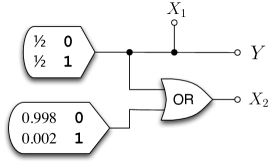
(b) circuit diagram

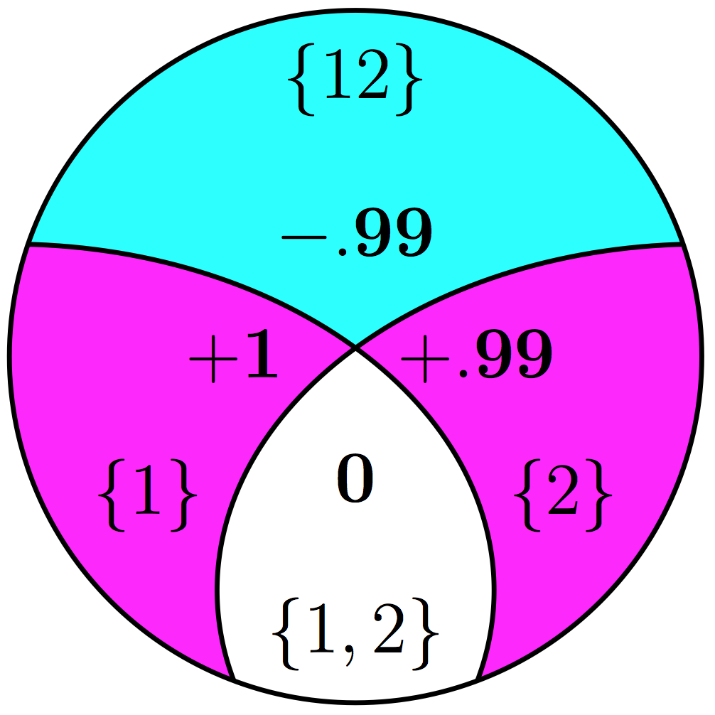
(c) $\operatorname{I}_{\wedge}$

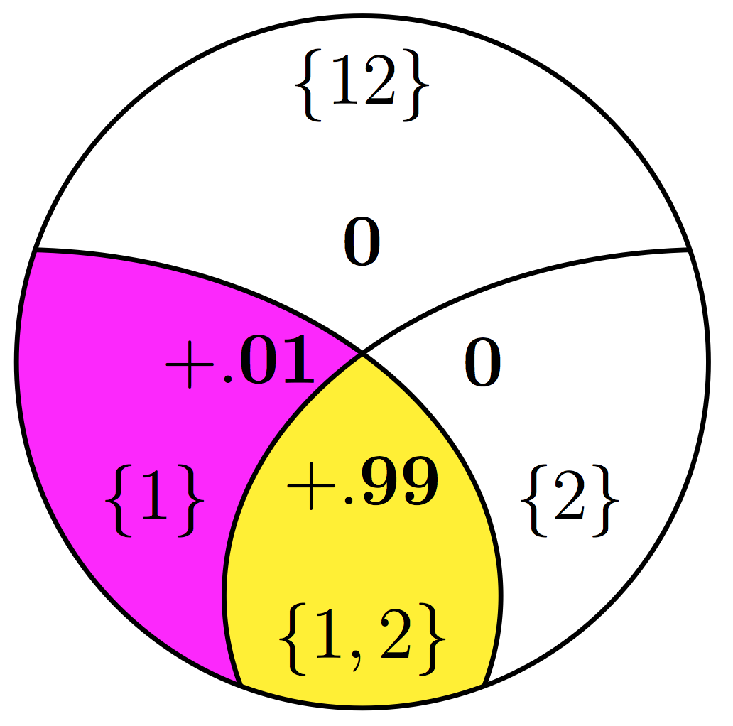
(d) Syn/$\Delta\operatorname{I}$/$\operatorname{I}_{\min}$/$\operatorname{I}_{\alpha}$

Figure 5: Example ImperfectRdn. $\operatorname{I}_{\wedge}$ is blind to the noisy correlation between $X_{1}$ and $X_{2}$ and calculates zero redundant information. An ideal $\operatorname{I}_{\cap}$ measure would detect that all of the information $X_{2}$ specifies about $Y$ is also specified by $X_{1}$ to calculate $\operatorname{I}_{\cap}\!\left(\{X_{1},X_{2}\}\!\mathrel{\mathop{\mathchar 58\relax}}\!Y\right)=0.99$ bits.

IV Previous candidate measures

In [13], the authors propose to use the following quantity, $\operatorname{I}_{\min}$, as the intersection information measure:

$$\begin{split}&\operatorname{I}_{\min}\left(X_{1},\ldots,X_{n}\mathrel{\mathop{\mathchar 58\relax}}Y\right)\\ &\equiv\sum_{y\in Y}\Pr\!\left(y\right)\min_{i\in\{1,\ldots,n\}}\operatornamewithlimits{I}\!\left(X_{i}\!\mathrel{\mathop{\mathchar 58\relax}}\!Y=y\right)\\ &=\sum_{y\in Y}\Pr\!\left(y\right)\min_{i\in\{1,\ldots,n\}}\operatorname{D_{KL}}\!\left[\Pr\!\left(X_{i}|y\right)\middle\|\,\Pr\!\left(X_{i}\right)\right]\;,\end{split}$$ (3)

where $\operatorname{D_{KL}}$ is the Kullback-Leibler divergence.

Though $\operatorname{I}_{\min}$ is an intuitive and plausible choice for the intersection information, [9] showed that $\operatorname{I}_{\min}$ has counterintuitive properties. In particular, $\operatorname{I}_{\min}$ calculates one bit of redundant information for example Unq (Figure 2). It does this because each input shares one bit of information with the output. However, its quite clear that the shared informations are, in fact, different: $X_{1}$ provides the low bit, while $X_{2}$ provides the high bit. This led to the conclusion that $\operatorname{I}_{\min}$ overestimates the ideal intersection information measure by focusing only on how much information the inputs provide to the output. Another way to understand why $\operatorname{I}_{\min}$ overestimates redundancy in example Unq is to imagine a hypothetical example where there are exactly two bits of unique information for every state $y\in Y$ and no synergy or redundancy. $\operatorname{I}_{\min}$ would calculate the redundancy as the minimum over both predictors which would be $\min[1,1]=1$ bit. Therefore $\operatorname{I}_{\min}$ would calculate $1$ bit of redundancy even though by definition there was no redundancy but merely two bits of unique information.

A candidate measure of synergy, $\Delta\operatorname{I}$, proposed in [14], leads to a negative value of redundant information for Example And. Starting from $\Delta\operatorname{I}$ as a direct measure for synergistic information and then using eqs. (1) and (2) to derive the other terms, we get Figure 4c showing $\operatorname{I}_{\cap}\!\left(\{X_{1},X_{2}\}\!\mathrel{\mathop{\mathchar 58\relax}}\!Y\right)\approx-.085$ bits.

Another candidate measure of synergy, Syn [15], calculates zero synergy and redundancy for Example RdnXor, as opposed to the intuitive value of one bit of redundancy and one bit of synergy.

V New candidate measures

V-A The $\operatorname{I}_{\wedge}$ measure

Based on [16], we can consider a candidate intersection information as the maximum mutual information $\operatornamewithlimits{I}\!\left(Q\!\mathrel{\mathop{\mathchar 58\relax}}\!Y\right)$ that some random variable $Q$ conveys about $Y$, subject to $Q$ being a function of each predictor $X_{1},\ldots,X_{n}$. After some algebra, the leads to,

$$\begin{split}&\operatorname{I}_{\wedge}\!\left(\{X_{1},\ldots,X_{n}\}\!\mathrel{\mathop{\mathchar 58\relax}}\!Y\right)\\ &\equiv\max_{\Pr(Q|Y)}\operatornamewithlimits{I}\!\left(Q\!\mathrel{\mathop{\mathchar 58\relax}}\!Y\right)\\ &\hskip 14.45377pt\textnormal{subject to }\forall i\in\{1,\ldots,n\}\mathrel{\mathop{\mathchar 58\relax}}\operatornamewithlimits{H}\!\left(Q|X_{i}\right)=0\end{split}\;,$$ (4)

which reduces to a simple expression in [12].

Example ImperfectRdn highlights the foremost shortcoming of $\operatorname{I}_{\wedge}$; $\operatorname{I}_{\wedge}$ does not detect “imperfect” or “lossy” correlations between $X_{1}$ and $X_{2}$. Instead, $\operatorname{I}_{\wedge}$ calculates zero redundant information, that $\operatorname{I}_{\cap}\!\left(\{X_{1},X_{2}\}\!\mathrel{\mathop{\mathchar 58\relax}}\!Y\right)=0$ bits. This arises from $\Pr\!\left(X_{1}=\texttt{1},X_{2}=\texttt{0}\right)>0$. If this were zero, ImperfectRdn reverts to being determined by the properties $\mathbf{(SR)}$ and the $\mathbf{\left(M_{0}\right)}$ equality condition. Due to the nature of the common random variable, $\operatorname{I}_{\wedge}$ only sees the “deterministic” correlations between $X_{1}$ and $X_{2}$—add even an iota of noise between $X_{1}$ and $X_{2}$ and $\operatorname{I}_{\wedge}$ plummets to zero. This highlights a related issue with $\operatorname{I}_{\wedge}$; it is not continuous—an arbitrarily small change in the probability distribution can result in a discontinuous jump in the value of $\operatorname{I}_{\wedge}$.

Despite this, $\operatorname{I}_{\wedge}$ is useful stepping-stone, it captures what is inarguably redundant information (the common random variable). In addition, unlike earlier measures, $\operatorname{I}_{\wedge}$ satisfies $\mathbf{(TM)}$.

V-B The $\operatorname{I}_{\alpha}$ measure

Intuitively, we expect that if $Q$ only specifies redundant information, that conditioning on any predictor $X_{i}$ would vanquish all of the information $Q$ conveys about $Y$. Noticing that $\operatorname{I}_{\wedge}$ underestimates the ideal $\operatorname{I}_{\cap}$ measure (i.e. it doesn’t satisfy $\mathbf{(LP)}$), we loosen the constraint $\operatornamewithlimits{H}\!\left(Q|X_{i}\right)=0$ in eq. (4), leading us to define the measure $\operatorname{I}_{\alpha}$:

$$\begin{split}&\operatorname{I}_{\alpha}\!\left(\{X_{1},\ldots,X_{n}\}\mathrel{\mathop{\mathchar 58\relax}}Y\right)\\ &\equiv\max_{\Pr(Q|Y)}\operatornamewithlimits{I}\!\left(Q\!\mathrel{\mathop{\mathchar 58\relax}}\!Y\right)\\ &\hskip 14.45377pt\textnormal{subject to }\forall i\in\{1,\ldots,n\}\mathrel{\mathop{\mathchar 58\relax}}\operatornamewithlimits{I}\!\left(Q,X_{i}\!\mathrel{\mathop{\mathchar 58\relax}}\!Y\right)=\operatornamewithlimits{I}\!\left(X_{i}\!\mathrel{\mathop{\mathchar 58\relax}}\!Y\right)\;.\end{split}$$ (5)

$$\begin{split}&=\max_{\Pr(Q|Y)}\operatornamewithlimits{I}\!\left(Q\!\mathrel{\mathop{\mathchar 58\relax}}\!Y\right)\\ &\hskip 14.45377pt\textnormal{subject to }\forall i\in\{1,\ldots,n\}\mathrel{\mathop{\mathchar 58\relax}}\operatornamewithlimits{H}\!\left(Q\middle|X_{i}\right)=\operatornamewithlimits{H}\!\left(Q\middle|X_{i},Y\right)\;.\end{split}$$ (6)

This measure obtains the desired values for the canonical examples in Section III. However, its implicit definition makes it more difficult to verify whether or not it satisfies the desired properties in Section III. Pleasingly, $\operatorname{I}_{\alpha}$ also satisfies $\mathbf{(TM)}$.

We can also show (See Lemmas 1 and 2 in Appendix References) that

$$\begin{split}&0\leq\operatorname{I}_{\wedge}\!\left(\{X_{1},\ldots,X_{n}\}\!\mathrel{\mathop{\mathchar 58\relax}}\!Y\right)\leq\operatorname{I}_{\alpha}\!\left(\{X_{1},\ldots,X_{n}\}\mathrel{\mathop{\mathchar 58\relax}}Y\right)\\ &\leq\operatorname{I}_{\min}\left(X_{1},\ldots,X_{n}\mathrel{\mathop{\mathchar 58\relax}}Y\right)\;.\end{split}$$ (7)

While $\operatorname{I}_{\alpha}$ satisfies previously defined canonical examples, we have found another example, shown in Figure 6, for which $\operatorname{I}_{\wedge}$ and $\operatorname{I}_{\alpha}$ both calculate negative synergy. This example further complicates Example And by making the predictors mutually dependent.

$\ \,X_{1}\,X_{2}$	$Y$
0 0	00	$\nicefrac{{1}}{{3}}$
0 1	01	$\nicefrac{{1}}{{3}}$
1 1	11	$\nicefrac{{1}}{{3}}$

(a) $\Pr\!\left(x_{1},x_{2},y\right)$

$$\operatornamewithlimits{I}\!\left(X_{1},X_{2}\!\mathrel{\mathop{\mathchar 58\relax}}\!Y\right) =1.585$$

$$\operatornamewithlimits{I}\!\left(X_{1}\!\mathrel{\mathop{\mathchar 58\relax}}\!Y\right) =0.918$$

$$\operatornamewithlimits{I}\!\left(X_{2}\!\mathrel{\mathop{\mathchar 58\relax}}\!Y\right) =0.918$$

$$\operatornamewithlimits{I}\!\left(X_{1}\!\mathrel{\mathop{\mathchar 58\relax}}\!X_{2}\right) =0.252$$

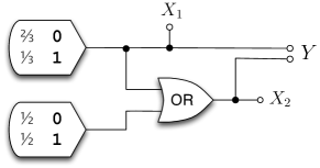
(b) circuit diagram

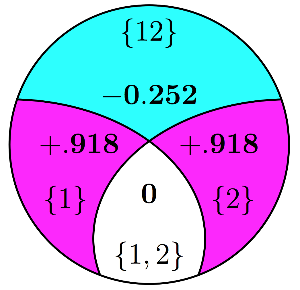
(c) $\operatorname{I}_{\wedge}$/$\operatorname{I}_{\alpha}$

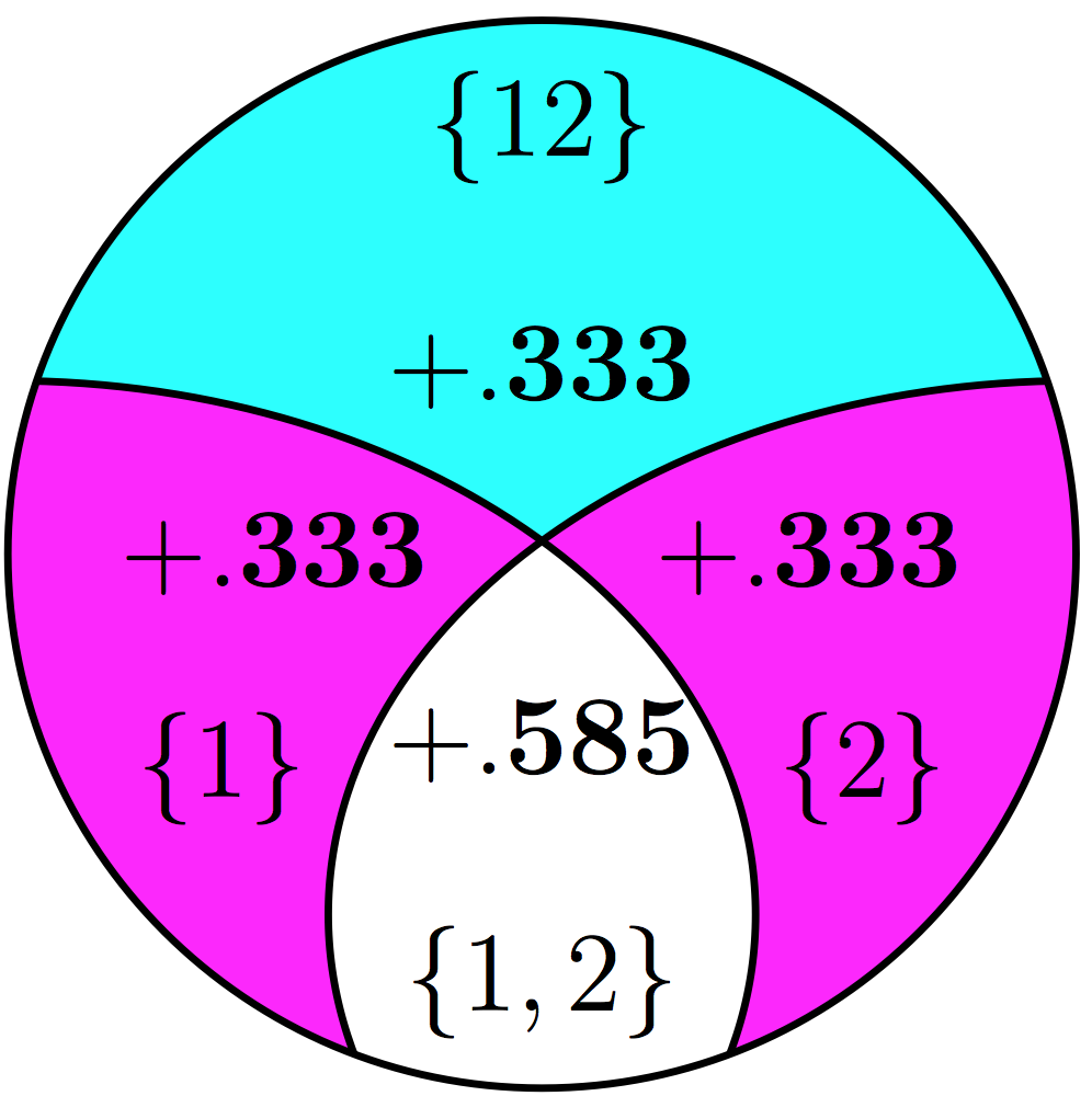
(d) $\operatorname{I}_{\min}$

Figure 6: Example Subtle.

VI Conclusion

We have defined new measures for redundant information of predictor random variables regarding a target random variable. It is not clear whether it is possible for a single measure of synergy/redundancy to satisfy all previously proposed desired properties and canonical examples, and some of them are debatable. For example, a plausible measure of the “unique information” [17] and “union information” [9] yields an equivalent $\operatorname{I}_{\cap}$ measure that does not satisfy $\mathbf{(TM)}$. Determining whether some of these properties are contradictory is an interesting question for further work.

Acknowledgements. We thank Jim Beck, Yaser Abu-Mostafa, Edwin Chong, Chris Ellison, and Ryan James for helpful discussions.

Proof $\operatorname{I}_{\alpha}$ does not satisfy $\mathbf{(LP)}$. Proof by counter-example Subtle (Figure 6). For $\operatornamewithlimits{I}\!\left(Q\!\mathrel{\mathop{\mathchar 58\relax}}\!Y|X_{1}\right)=0$, then $Q$ must not distinguish between states of $Y=\texttt{00}$ and $Y=\texttt{01}$ (because $X_{1}$ does not distinguish between these two states). This entails that $\Pr\!\left(Q|Y=\texttt{00}\right)=\Pr\!\left(Q|Y=\texttt{01}\right)$. By symmetry, likewise for $\operatornamewithlimits{I}\!\left(Q\!\mathrel{\mathop{\mathchar 58\relax}}\!Y|X_{2}\right)=0$, $Q$ must be distinguish between states $Y=\texttt{01}$ and $Y=\texttt{11}$. Altogether, this entails that $\Pr\!\left(Q|Y=\texttt{00}\right)=\Pr\!\left(Q|Y=\texttt{01}\right)=\Pr\!\left(Q|Y=\texttt{11}\right)$, which then entails, $\Pr\!\left(q|y_{i}\right)=\Pr\!\left(q|y_{j}\right)\quad\forall q\in Q,y_{i}\in Y,y_{j}\in Y$, which is only achievable when $\Pr\!\left(q\right)=\Pr\!\left(q|y\right)\quad\forall q\in Q,y\in Y$. This makes $\operatornamewithlimits{I}\!\left(Q\!\mathrel{\mathop{\mathchar 58\relax}}\!Y\right)=0$, therefore for example Subtle, $\operatorname{I}_{\alpha}\!\left(\{X_{1},X_{2}\}\mathrel{\mathop{\mathchar 58\relax}}Y\right)=0$.

Lemma 1.

We have $\operatorname{I}_{\wedge}\!\left(\{X_{1},\ldots,X_{n}\}\!\mathrel{\mathop{\mathchar 58\relax}}\!Y\right)\leq\operatorname{I}_{\alpha}\!\left(\{X_{1},\ldots,X_{n}\}\mathrel{\mathop{\mathchar 58\relax}}Y\right)$.

Proof.

We define a random variable $Q^{\prime}=X_{1}\wedge\cdots\wedge X_{n}$. We then plugin $Q^{\prime}$ for $Q$ in the definition of $\operatorname{I}_{\alpha}$. This newly plugged-in $Q$ satisfies the constraint $\forall i\in\{1,\ldots,n\}$ that $\operatornamewithlimits{I}\!\left(Q\!\mathrel{\mathop{\mathchar 58\relax}}\!Y|X_{i}\right)=0$. Therefore, $Q^{\prime}$ is always a possible choice for $Q$, and the maximization of $\operatornamewithlimits{I}\!\left(Q\!\mathrel{\mathop{\mathchar 58\relax}}\!Y\right)$ in $\operatorname{I}_{\alpha}$ must be at least as large as $\operatornamewithlimits{I}\!\left(Q^{\prime}\!\mathrel{\mathop{\mathchar 58\relax}}\!Y\right)=\operatorname{I}_{\wedge}\!\left(\{X_{1},\ldots,X_{n}\}\!\mathrel{\mathop{\mathchar 58\relax}}\!Y\right)$. ∎

Lemma 2.

We have $\operatorname{I}_{\alpha}\!\left(\{X_{1},\ldots,X_{n}\}\mathrel{\mathop{\mathchar 58\relax}}Y\right)\leq\operatorname{I}_{\min}\left(X_{1},\ldots,X_{n}\mathrel{\mathop{\mathchar 58\relax}}Y\right)$

Proof.

For a given state $y\in Y$ and two arbitrary random variables $Q$ and $X$, given $\operatornamewithlimits{I}\!\left(Q\!\mathrel{\mathop{\mathchar 58\relax}}\!y|X\right)=\operatorname{D_{KL}}\!\left[\Pr\!\left(QX|y\right)\middle\|\,\Pr\!\left(Q|X\right)\Pr\!\left(X|y\right)\right]=0$, we show that, $\operatornamewithlimits{I}\!\left(Q\!\mathrel{\mathop{\mathchar 58\relax}}\!y\right)\leq\operatornamewithlimits{I}\!\left(X\!\mathrel{\mathop{\mathchar 58\relax}}\!y\right)$,

$$\operatornamewithlimits{I}\!\left(X\!\mathrel{\mathop{\mathchar 58\relax}}\!y\right)-\operatornamewithlimits{I}\!\left(Q\!\mathrel{\mathop{\mathchar 58\relax}}\!y\right) =\sum_{x\in X}\Pr\!\left(x|y\right)\log\frac{\Pr\!\left(x|y\right)}{\Pr\!\left(x\right)}-\sum_{q\in Q}\Pr\!\left(q|y\right)\log\frac{\Pr\!\left(q|y\right)}{\Pr\!\left(q\right)}$$

$$\geq 0\;.$$

Generalizing to $n$ predictors $X_{1},\ldots,X_{n}$, the above shows that that the maximum $\operatornamewithlimits{I}\!\left(Q\!\mathrel{\mathop{\mathchar 58\relax}}\!y\right)$ under constraint $\operatornamewithlimits{I}\!\left(Q\!\mathrel{\mathop{\mathchar 58\relax}}\!y|X_{i}\right)$ will always be less than $\min_{i\in\{1,\ldots,n\}}\operatornamewithlimits{I}\!\left(X_{i}\!\mathrel{\mathop{\mathchar 58\relax}}\!y\right)$, which completes the proof. ∎

Lemma 3.

Measure $\operatorname{I}_{\min}$ satisfies desired property Strong Monotonicity, $\mathbf{\left(M_{1}\right)}$.

Proof.

Given $\operatornamewithlimits{H}\!\left(Y|Z\right)=0$, then the specific-surprise $\operatornamewithlimits{I}\!\left(Z\!\mathrel{\mathop{\mathchar 58\relax}}\!y\right)$ yields,

$$\operatornamewithlimits{I}\!\left(Z\!\mathrel{\mathop{\mathchar 58\relax}}\!y\right) \equiv \operatorname{D_{KL}}\!\left[\Pr\!\left(Z|y\right)\middle\|\,\Pr\!\left(Z\right)\right]$$

$$= \sum_{z\in Z}\Pr\!\left(z|y\right)\log\frac{\Pr\!\left(z|y\right)}{\Pr\!\left(z\right)}$$

$$= \sum_{z\in Z}\Pr\!\left(z|y\right)\log\frac{1}{\Pr\!\left(y\right)}$$

$$= \log\frac{1}{\Pr\!\left(y\right)}\;.$$

Given that for an arbitrary random variable $X_{i}$, $\operatornamewithlimits{I}\!\left(X_{i}\!\mathrel{\mathop{\mathchar 58\relax}}\!y\right)\leq\log\frac{1}{\Pr\!\left(y\right)}$. As $\operatorname{I}_{\min}$ takes only uses the $\min_{i}\operatornamewithlimits{I}\!\left(X_{i}\!\mathrel{\mathop{\mathchar 58\relax}}\!y\right)$, the minimum is invariant under adding any predictor $Z$ such that $\operatornamewithlimits{H}\!\left(Y|Z\right)=0$. Therefore, measure $\operatorname{I}_{\min}$ satisfies property $\mathbf{\left(M_{1}\right)}$. ∎

References

[1]
Schneidman E, Bialek W, II MB (2003) Synergy, redundancy, and independence in
population codes.
Journal of Neuroscience 23: 11539–53.
[2]
Narayanan NS, Kimchi EY, Laubach M (2005) Redundancy and synergy of neuronal
ensembles in motor cortex.
The Journal of Neuroscience 25: 4207-4216.
[3]
Balduzzi D, Tononi G (2008) Integrated information in discrete dynamical
systems: motivation and theoretical framework.
PLoS Computational Biology 4: e1000091.
[4]
Anastassiou D (2007) Computational analysis of the synergy among multiple
interacting genes.
Molecular Systems Biology 3: 83.
[5]
Lizier JT, Flecker B, Williams PL (2013) Towards a synergy-based approach to
measuring information modification.
CoRR abs/1303.3440.
[6]
Gács P, Körner J (1973) Common information is far less than mutual
information.
Problems of Control and Informaton Theory 2: 149–162.
[7]
Wyner AD (1975) The common information of two dependent random variables.
IEEE Transactions in Information Theory 21: 163–179.
[8]
Kumar GR, Li CT, Gamal AE (2014) Exact common information.
CoRR abs/1402.0062.
[10]
Harder M, Salge C, Polani D (2013) Bivariate measure of redundant information.
Phys Rev E 87: 012130.
[11]
Bertschinger N, Rauh J, Olbrich E, Jost J (2012) Shared information – new
insights and problems in decomposing information in complex systems.
CoRR abs/1210.5902.
[12]
Griffith V, Chong EKP, James RG, Ellison CJ, Crutchfield JP (2013) Intersection
information based on common randomness.
CoRR abs/1310.1538.
[13]
Williams PL, Beer RD (2010) Nonnegative decomposition of multivariate
information.
CoRR abs/1004.2515.
[14]
Nirenberg S, Latham PE (2003) Decoding neuronal spike trains: How important are
correlations?
Proceedings of the National Academy of Sciences 100: 7348–7353.
[15]
Schneidman E, Still S, Berry MJ, Bialek W (2003) Network information and
connected correlations.
Phys Rev Lett 91: 238701-238705.
[16]
Wolf S, Wullschleger J (2004) Zero-error information and applications in
cryptography.
Proc IEEE Information Theory Workshop 04: 1–6.
[17]
Bertschinger N, Rauh J, Olbrich E, Jost J, Ay N (2013) Quantifying unique
information.
CoRR abs/1311.2852.