Effective Simulation Methods for Structures with Local Nonlinearity: Magnus integrator and Successive Approximations

Abstract

In the following, we discuss nonlinear simulations of nonlinear dynamical systems, which are applied in technical and biological models. We deal with different ideas to overcome the treatment of the nonlinearities and discuss a novel splitting approach. While Magnus expansion has been intensely studied and widely applied for solving explicitly time-dependent problems, it can also be extended to nonlinear problems. By the way it is delicate to extend, while an exponential character have to be computed. Alternative methods, like successive approximation methods, might be an attractive tool, which take into account the temporally in-homogeneous equation (method of Tanabe and Sobolevski). In this work, we consider nonlinear stability analysis with numerical experiments and compare standard integrators to our novel approaches.

Keywords: Magnus Integrator, successive approximation, exponential splitting, Fisher’s equation, nonlinear dynamical models, nonlinear methods.

AMS subject classifications. 65M15, 65L05, 65M71.

1 Introduction

In this paper, we concentrate on solving nonlinear evolution equations, which arose in nonlinear dynamical applications, e.g., biological growth regimes or plasma simulations. We apply the following nonlinear differential equation,

$$\partial_{t}\;u=A_{1}u+A_{2}(u),\;u(0)=u_{0},$$ (1)

where $A_{1}$ is the linear operator, while $A_{2}(u)$ is the nonlinear operator.

To solve such delicate nonlinear differential equations, we have different approaches:

• Approximation of the nonlinear term via time-dependent terms (Magnus expension).

• Approximation of the nonlinear terms via multiscale expensions (successive approximation).

The Magnus expansion [2] is an attractive and widely applied method of solving explicitly time-dependent problems. However, it requires computing time-integrals and nested commutators to higher orders. Successive approximation is based on recursive integral formulations in which an iterative method is enforce the time dependency.

The paper is outlined as follows: In Section 2, we summarizes the Magnus expansion and its application to Hamiltonian systems. Further, we show how AB-, Verlet and successive approximation method can be applied to any exponential-splitting algorithms in Section 3. In Section 4 we present the numerical results of the splitting schemes. In Section 5, we briefly summarize our results.

2 Introduction to splitting methods

For nonlinear problems, the applications of splitting methods are more delicate because of resolving the nonlinear operators. We apply a nonlinear approach based on Magnus expansion and successive approximations.

We concentrate on approximation to the solution of the nonlinear evolution equation, e.g. time-dependent Schrödinger equation,

$$\partial_{t}\;u=F(u(t))+g(u)=Au(t)+B(u(t))u(t)+g(u),\;u(0)=u_{0},$$ (2)

with the unbounded operators $A:D(A)\subset{\bf X}\rightarrow{\bf X}$ and $B:D(B)\subset{\bf X}\rightarrow{\bf X}$. We have further $F(v)=A(v)+B(v),v\in D(A)\cap D(B)$ and $g(u)$ is a nonlinear function.

We assume to have suitable chosen sub-spaces of the underlying Banach space $(X,||\cdot||_{X})$ such that $D(F)=D(A)\cap D(B)\neq\emptyset$

The exact solution of the evolution problem 2 is given as:

$$u(t)={\cal E}_{F}(t,u(0))+\int_{0}^{t}{\cal E}_{F}(t-\tau,g(u(\tau))d\tau,\;0\leq t\leq T,$$ (3)

with the evolution operator ${\cal E}_{F}$ depending on the actual time $t$ and the initial value $u(0)$.

Example 2.1.

For the linear case, means $F(u)=Au+Bu$ the evolution operator is given as:

$$u(t)=\exp(tD_{F})u(0)+\int_{0}^{t}\exp((t-\tau)D_{F})g(u(\tau))d\tau,\;0\leq t\leq T,$$ (4)

with $D_{F}=A+B$.

In the next subsections, we introduce the underlying splitting methods.

3 Nonlinear Splitting Method

We apply the abstract standard splitting schemes to the multiproduct decomposition.

We have to carry out the following steps:

• Apply the nonlinear Strang splitting scheme,

• embed the Strang splitting scheme into the multiproduct expansion.

To apply the abstract setting of a nonlinear Magnus expansion, we deal with the following modified nonlinear equation

$$\partial_{t}u=Au(t)+B(t,u(t))u(t),\qquad u(0)=u_{0},$$ (5)

where $A,B(t,u)\in[0,T]\times{\bf X}$ are non-commuting operators, ${\bf X}$ is a general Banach space, e.g., ${\bf X}\subset{\rm I}\!{\rm R}^{m}$, where $m$ is the rank of the matrices.

To apply the nonlinear Magnus expansion, we deal with:

$$\partial_{t}u=B(t,u(t))u(t),\qquad u(0)=u_{0},\\ u(t)=\exp(\Omega_{B}(t,u_{0}))u_{0},\\$$ (6)

where the first order Magnus operator is given by Euler’s formula:

$$\Omega_{B,1}(t,u_{0})=\int_{0}^{t}B(s,u(s))ds=t\;B(0,u_{0}),$$ (7)

and the second order Magnus operator is given by the midpoint rule:

$$\Omega_{B,2}(t,u_{0}) = \int_{0}^{t}B(s,\exp(\Omega_{B,1}(s,u_{0})))ds,$$

$$= tB(\frac{t}{2},\exp(\Omega_{B,1}(\frac{t}{2},u_{0})))$$

$$= tB(\frac{t}{2},\frac{t}{2}B(0,u_{0})),$$

or Trapezoidal-rule:

$$\Omega_{B,2}(t,u_{0}) = \int_{0}^{t}B(s,\exp(\Omega_{B,1}(s,u_{0})))ds,$$

$$= t/2\left(B(0,u_{0})+B(t,\exp(tB(0,u_{0})u_{0}))\right).$$

We can generalize the schemes with respect to more additional terms to higher order schemes, see [4]

• We apply the following A-B splitting scheme:

  $$\partial_{t}u_{1}=Au_{1}(t),\qquad u(t^{n})=u_{n},$$ (10)

  $$\partial_{t}u_{2}=B(t,u_{2}(t))u_{2}(t),\qquad u_{2}(t^{n})=u_{1}(t^{n+1}),$$ (11)

  where the time-step is $\Delta t=t^{n+1}-t^{n}$ and the next solution is:
  $u(t^{n+1})=u_{2}(t^{n+1})$.

  Here we apply the kernels:

  $$u_{2}(t^{n+1})=\exp(\Omega_{B,2}(\Delta t,u_{1}(t^{n+1})))u_{1}(t^{n+1}),$$ (12)

  $$u_{1}(t^{n+1})=\exp(A\Delta t)u(t^{n})$$ (13)

  We have:

  $${\cal T}_{1,BA}(\Delta t)u(t^{n}) = \exp(\Omega_{B,2}(\Delta t,\exp(A\Delta t)u(t^{n})))\exp(A\Delta t)u(t^{n}),$$ (14)

• Verlet Splitting (Strang-Splitting)

  We apply two A-B splitting, means:

  $${\cal T}_{1,AB}(\Delta t)u(t^{n}) = \exp(A\Delta t)\exp(\Omega_{B,1}(\Delta t,u(t^{n}))),$$ (15)

  $${\cal T}_{1,BA}(\Delta t)u(t^{n}) = \exp(\Omega_{B,2}(\Delta t,\exp(A\Delta t)u(t^{n})))\exp(A\Delta t)u(t^{n}),$$ (16)

  where $\Omega_{A,i},\Omega_{B,i}$ are the Magnus expansions, see equations (7) and (3), of order $i$ and we obtain: the scheme based on the symmetrical splitting by

  $${\cal T}_{2}(\Delta t)u(t^{n}) = {\cal T}_{1,BA}(\frac{\Delta t}{2}){\cal T}_{1,AB}(\frac{\Delta t}{2})u(t^{n}).$$ (17)

• Standard Successive Approximation via linear operator $A$ (without multiscale approximation)

  We deal with the equation:

  $$\frac{\partial u(t)}{\partial t}=Au(t)\;+\;B(t,u(t))u(t),\;\mbox{with}\;\;u(0)=u_{init}(0).$$ (18)

  Then the successive equations are given as:

  $$\frac{\partial u_{0}(t)}{\partial t}=Au_{0}(t),\;u_{0}(t^{n})=u(t^{n}),\;t\in[t^{n},t^{n+1}],$$ (19)

  $$\frac{\partial u_{1}(t)}{\partial t}=Au_{1}(t)+\;B(u_{0}(t))u_{0}(t),\;u_{1}(t^{n})=u(t^{n}),\;t\in[t^{n},t^{n+1}],$$ (20)

  $$\frac{\partial u_{2}(t)}{\partial t}=Au_{2}(t)+\;B(u_{2}(t))u_{1}(t),\;u_{0}(t^{n})=u(t^{n}),\;t\in[t^{n},t^{n+1}],$$ (21)

  $$\frac{\partial u_{3}(t)}{\partial t}=Au_{3}(t)+\;B(u_{2}(t))u_{2}(t),\;u_{3}(t^{n})=u(t^{n}),\;t\in[t^{n},t^{n+1}],$$ (22)

  $$\vdots$$

  where $\Delta t=t^{n+1}-t^{n}$, we start with $u(0)=u_{init}(0)$, the successive solution at $t^{n+1}$ with $i=3$ steps are given as $u(t^{n+1})=u_{3}(t^{n+1})$.

  By integration, we have the following solutions, we start with $n=0$ and $u(0)=u(t^{0})=u_{init}(0)$:

  $$u_{0}(t^{n+1}) = \exp(A\Delta t)u(t^{n}),$$ (23)

  $$u_{1}(t^{n+1}) = \exp(A\Delta t)u(t^{n})$$ (24)

  $$+\int_{t^{n}}^{t^{n+1}}\exp(A(t^{n+1}-s))\;B(u_{0}(s))\;u_{0}(s)\;ds,$$

  $$u_{2}(t^{n+1}) = \exp(A\Delta t)u(t^{n})$$ (25)

  $$+\int_{t^{n}}^{t^{n+1}}\exp(A(t^{n+1}-s))B(u_{1}(s))u_{1}(s)\;ds,$$

  with $\Delta t=t^{n+1}-t^{n}$ is the time step.

  We apply a simple trapezoidal-rule to the integrals and obtain:

  $$\tilde{u}_{1}(t^{n+1})=\frac{\Delta t}{2}\left(B(u_{0}(t^{n+1}))\;u_{0}(t^{n+1})\right.$$ (26)

  $$\left.+\exp(A\Delta t)B(u_{0}(t^{n}))\;u_{0}(t^{n})\right),$$

  $$\tilde{u}_{2}(t^{n+1})=\frac{\Delta t}{2}\left(B(u_{1}(t^{n+1}))u_{1}(t^{n+1})\right.$$ (27)

  $$\left.+\exp(A\;\Delta t)B(u_{1}(t^{n}))u_{1}(t^{n})\right),$$

  where we applied mid-point rule or Simpson’s-rule, then we have for $3$ iterative steps, $u(t^{n+1})$ is given as

  $$u(t^{n+1})=u_{0}(t^{n+1})+\tilde{u}_{1}(t^{n+1})+\tilde{u}_{2}(t^{n+1}).$$ (28)

• Successive Approximation via linear operator $A$ (Multiscale expansion)

  We deal with the multiscale idea:

  $$\frac{\partial u(t)}{\partial t}=Au(t)\;+\;\epsilon\;B(t,u(t))u(t),\;\mbox{with}\;\;u(0)=u_{init}(0),$$ (29)

  where $0<\epsilon\leq 1$. For $\epsilon\rightarrow 1$, we have the original equation.

  We derive a solutions $u(t,\epsilon)$ and apply:

  $$u(t,\epsilon)=u_{0}(t)+\epsilon u_{1}(t)+\epsilon^{2}u_{2}(t)+\ldots+\epsilon^{J}u_{J}(t),$$ (30)

  with the initial conditions $u(0,\epsilon)=u(0)$ and $J\in{I\!\!N}^{+}$ is a fixed iteration number.

  Then the hierarchical equations are given as:

  $$\frac{\partial u_{0}(t)}{\partial t} = Au_{0}(t),\;u_{0}(t^{n})=u(t^{n}),t\in[t^{n},t^{n+1}],$$ (31)

  $$\frac{\partial u_{1}(t)}{\partial t} = Au_{1}(t)+\;B(u_{0}(t))u_{0}(t),$$

  $$\;u_{1}(t^{n})=u(t^{n}),t\in[t^{n},t^{n+1}],$$

  $$\frac{\partial u_{2}(t)}{\partial t} = Au_{2}(t)$$

  $$+\;B(u_{0}(t))u_{1}(t)+\;B^{\prime}(u_{0}(t))u_{1}(t)u_{0}(t),$$

  $$\;u_{2}(t^{n})=u(t^{n}),t\in[t^{n},t^{n+1}],$$

  $$\frac{\partial u_{3}(t)}{\partial t} = Au_{3}(t)+\;B(u_{0}(t))u_{2}(t)+\;B^{\prime}(u_{0}(t))u_{2}(t)u_{0}(t)$$

  $$+\;B^{\prime}(u_{0}(t))u_{1}(t)u_{1}(t)+\;B^{\prime\prime}(u_{0}(t))u_{1}(t)u_{1}(t)u_{0}(t),$$

  $$\;u_{3}(t^{n})=u(t^{n}),t\in[t^{n},t^{n+1}],$$

  $$\vdots$$

  where we extend $B(u_{0}(t)+\epsilon(u_{1}(t)+\epsilon u_{2}(t)+\ldots))=B(u_{0}(t))+\epsilon(u_{1}(t)+\epsilon u_{2}(t)+\ldots)B^{\prime}(u_{0})+(\epsilon(u_{1}(t)+\epsilon u_{2}(t)+\ldots))^{2}B^{\prime\prime}(u_{0})*\ldots$ with $B^{\prime}(u_{0})=\frac{\partial B(u)}{\partial u}|_{u=u_{0}}$ and $B^{\prime\prime}(u_{0})=\frac{\partial^{2}B(u)}{\partial u^{2}}|_{u=u_{0}}$. We have also to expand the initial conditions to $u_{0}(0)=u_{init}(0)$ and $u_{j}(0)=0,\;\forall j=1,\ldots,J$.

  By integration, we have the following solutions, we start with $n=0$ and $u(0)=u(t^{0})=u_{init}(0)$:

  $$u_{0}(t^{n+1}) = \exp(A\Delta t)u(t^{n}),$$ (35)

  $$u_{1}(t^{n+1}) = \exp(A\Delta t)u(t^{n})+\int_{t^{n}}^{t^{n+1}}\exp(A(t^{n+1}-s))\;B(u_{0}(s))\;u_{0}(s)\;ds,$$ (36)

  $$u_{2}(t^{n+1}) = \exp(A\Delta t)u(t^{n})$$

  $$+\int_{t^{n}}^{t^{n+1}}\exp(A(t^{n+1}-s))\left(B(u_{0}(s))u_{1}(s)+\;B^{\prime}(u_{0}(s))u_{1}(s)u_{0}(s)\right)\;ds,$$

  with $\Delta t=t^{n+1}-t^{n}$ is the time step.

  We apply a simple trapezoidal-rule to the integrals and obtain:

  $$\tilde{u}_{1}(t^{n+1})=\frac{\Delta t}{2}\left(B(u_{0}(t^{n+1}))\;u_{0}(t^{n+1})+\exp(A\Delta t)B(u_{0}(t^{n}))\;u_{0}(t^{n})\right),$$ (39)

  $$\tilde{u}_{2}(t^{n+1})=\frac{\Delta t}{2}\left(\left(B(u_{0}(t^{n+1}))u_{1}(t^{n+1})+\;B^{\prime}(u_{0}(t^{n+1}))u_{1}(t^{n+1})u_{0}(t^{n+1})\right)\right.$$

  $$\left.+\exp(A\;\Delta t)\left(B(u_{0}(t^{n}))u_{1}(t^{n})+\;B^{\prime}(u_{0}(t^{n}))u_{1}(t^{n})u_{0}(t^{n})\right)\right),$$

  where we also can apply mid-point rule or Simpson’s-rule, then we have for $u(t^{n+1})$

  $$u(t^{n+1})=u_{0}(t^{n+1})+\tilde{u}_{1}(t^{n+1})+\tilde{u}_{2}(t^{n+1})+\tilde{u}_{3}(t^{n+1}),$$ (40)

• Successive Approximation via linear operator $B$ (multiscale expansion)

  We deal with the multiscale idea:

  $$\frac{\partial u(t)}{\partial t}=\epsilon\;Au(t)\;+\;B(t,u(t))u(t),\;\mbox{with}\;\;u(0)=u_{init}(0),$$ (41)

  where $0<\epsilon\leq 1$. For $\epsilon\rightarrow 1$, we have the original equation.

  We derive a solutions $u(t,\epsilon)$ and apply:

  $$u(t,\epsilon)=u_{0}(t)+\epsilon u_{1}(t)+\epsilon^{2}u_{2}(t)+\ldots+\epsilon^{J}u_{J}(t),$$ (42)

  with the initial conditions $u(0,\epsilon)=u(0)$ and $J\in{I\!\!N}^{+}$ is a fixed iteration number.

  Then the hierarchical equations are given as:

  $$\frac{\partial u_{0}(t)}{\partial t} = B(u_{0}(t))u_{0}(t),\;u_{0}(t^{n})=u(t^{n}),$$ (43)

  $$\frac{\partial u_{1}(t)}{\partial t} = \left(B(u_{0}(t))+\;B^{\prime}(u_{0}(t))u_{0}(t)\right)u_{1}(t)+Au_{0}(t),$$

  $$\;u_{1}(t^{n})=u(t^{n}),$$

  $$\frac{\partial u_{2}(t)}{\partial t} = \;\left(B(u_{0}(t))u_{2}(t)+\;B^{\prime}(u_{0}(t))u_{0}(t)\right)u_{2}(t)$$

  $$+\;B^{\prime}(u_{0}(t))u_{1}(t)u_{1}(t)+\;B^{\prime\prime}(u_{0}(t))u_{1}(t)u_{1}(t)u_{0}(t)+Au_{1}(t),$$

  $$\;u_{2}(t^{n})=u(t^{n}),$$

  $$\vdots$$

  where the initialization is $u_{0}(0)=u_{init}(0)$ and we extend $B(u_{0}(t)+\epsilon(u_{1}(t)+\epsilon u_{2}(t)+\ldots))=B(u_{0}(t))+\epsilon(u_{1}(t)+\epsilon u_{2}(t)+\ldots)B^{\prime}(u_{0})+(\epsilon(u_{1}(t)+\epsilon u_{2}(t)+\ldots))^{2}B^{\prime\prime}(u_{0})*\ldots$ with $B^{\prime}(u_{0})=\frac{\partial B(u)}{\partial u}|_{u=u_{0}}$ and
  $B^{\prime\prime}(u_{0})=\frac{\partial^{2}B(u)}{\partial u^{2}}|_{u=u_{0}}$. We have also to expand the initial conditions to $u_{0}(0)=u_{init}(0)$ and $u_{j}(0)=0,\;\forall j=1,\ldots,J$.

  By integration, we have the following solutions, we start with $n=0$ and $u(0)=u(t^{0})=u_{init}(0)$:

  $$u_{0}(t^{n+1})=\exp(B(u(t^{n}))\Delta t)u(t^{n}),$$ (46)

  $$u_{1}(t^{n+1})=\exp(B(u_{0}(t^{n}))+B^{\prime}(u_{0}(t^{n}))\;u_{0}(t^{n}))u(t^{n})$$

  $$+\int_{t^{n}}^{t^{n+1}}\exp\left(\int_{s_{1}}^{t^{n+1}}B(u_{0}(s_{1}))+B^{\prime}(u_{0}(s_{1}))\;u_{0}(s_{1})\;ds_{1}\right)\;A\;u_{0}(s)\;ds,$$

  $$=\exp(B(u_{0}(t^{n}))+B^{\prime}(u_{0}(t^{n}))\;u_{0}(t^{n}))u(t^{n})$$ (47)

  $$+\int_{t^{n}}^{t^{n+1}}\exp\left(\left(B(u_{0}(s))+B^{\prime}(u_{0}(s))\;u_{0}(s)\right)\;(t^{n+1}-s)\right)\;A\;u_{0}(s)\;ds,$$

  with $\Delta t=t^{n+1}-t^{n}$ is the time step.

  We apply a simple trapezoidal-rule to the integrals and obtain:

  $$u_{1}(t^{n+1})=\frac{\Delta t}{2}\left(Au_{0}(t^{n+1})\right.$$

  $$\left.+\exp\left(\left(B(u_{0}(t^{n}))+B^{\prime}(u_{0}(t^{n}))\;u_{0}(t^{n})\right)\;\Delta t\right)\;A\;u_{0}(t^{n})\right),$$ (48)

  where we also can apply mid-point rule or Simpson’s-rule, then we have for $u(t^{n+1})$

  $$u(t^{n+1})=\tilde{u}_{0}(t^{n+1})+\tilde{u}_{1}(t^{n+1})=u_{1}(t^{n+1}),$$ (49)

Remark 3.1.

The benefit of the A-B and Strang-Splitting schemes are based on the explicit Magnus expansion and the fully decomposition of operator $A$ and $B$.

The benefit of the successive approximation scheme is the idea to skip the Magnus expansion and to deal with e relaxation over $B$. Here we have a weakly coupling based on the frozen solution (previous iterated solution) and we could deal only with matrix multiplications.

Remark 3.2.

While AB splitting has the idea to decompose into an A and B operator-equation, we have to compute for the A-equation $\exp(A)$ and for the B-equation the nonlinear $\exp(\int_{t^{n}}^{t^{n+1}}B(u(t))\;dt)$ part. The last term is expensive. The successive approximation has the following idea to iterate or perturb only to the A-operator, means we have the cheap part $\exp(A)$ and the integral part is only with the right-hand $B(u_{0}(t))$, that is given of the previous solution and there is no need to apply the Magnus-integrators for the exponential expension.

4 Numerical Experiments

In the following section, we deal with experiments to verify the benefit of our methods. At the beginning, we propose introductory examples to compare the methods. In the next examples, applications to nonlinear differential equations, as Bernoulli’s equation and Fisher’s equation for biological models.

4.1 First test example of a nonlinear ODE: Bernoulli’s equation

We deal with a nonlinear ODE (Bernoulli’s equation) and split it into linear and nonlinear operators.

First we examine the non linear Bernoulli-Equation

$$\frac{\partial u(t)}{\partial t} = \lambda_{1}u(t)+\lambda_{2}u^{n}(t)\;,$$ (50)

$$u(0) = 1\;,$$ (51)

with the analytic solution

$$u(t)=\left[(1+\frac{\lambda_{2}}{\lambda_{1}})\exp(\lambda_{1}t(1-n))-\frac{\lambda_{2}}{\lambda_{1}})\right]^{\frac{1}{1-n}}\;.$$ (52)

For the computations, we choose $n=2$ , $\lambda_{1}=-1$, $\lambda_{2}=-1,-2,-10$ and $\Delta t=10^{-2}$ .

We rewrite the equation-system (50) in operator notation, and obtain the following equations :

$$\partial_{t}u = Au+B(u)u\;,$$ (53)

$$u(0) = u_{0},$$ (54)

where $u(t)=(u_{1}(t),u_{2}(t))^{T}$ for $t\in[0,T]$.

Our split operators are

$$Au=\lambda_{1}u\;,\\ B(u)u=\lambda_{2}\;u^{m-1}u\;,$$ (55)

with $m=2$.

We also have a non-commutative behavior of the nonlinear operators, means $[A(u),B(u)]=\left(\frac{\partial B(u)}{\partial u}Au-\frac{\partial Au}{\partial u}B(u)\right)=\lambda_{2}(m-1)u^{m-2}\lambda_{2}u-\lambda_{1}\lambda_{2}u^{m-1}\neq 0$.

We have the following results with the $L_{2}$ and $L_{inf}$-error of our scheme, related to the analytic solution (52) in Figure 1 and 2.

Numerical Method	$err_{L_{2}}$	$err_{L_{inf}}$	Comput. time [sec]
AB-Splitting	$0.962$	$0.183$	$0.030$
Strang-splitting	$0.752$	$0.118$	$0.055$
Standard Successive	$0.283$	$0.100$	$0.013$
Multiscale Successive	$0.098$	$0.035$	$0.027$

Table 1: Numerical error of the different numerical methods for the Bernoulli’s equation.

Numerical Method	$\Delta t$	$err_{L_{2}}$	$err_{L_{inf}}$	Comput. time [sec]
Stand. Successive	$0.02$	0.260	0.096	0.002
Multi. Successive	$0.02$	0.087	0.032	0.004
AB-Splitting	$0.02$	0.800	0.173	0.017
Strang-splitting	$0.02$	0.588	0.110	0.011
Stand. Successive	$0.01$	0.160	0.039	0.004
Multi. Successive	$0.01$	0.026	0.007	0.009
AB-Splitting	$0.01$	1.154	0.177	0.011
Strang-splitting	$0.01$	0.826	0.109	0.018
Stand. Successive	$0.005$	0.106	0.018	0.008
Multi. Successive	$0.005$	0.008	0.002	0.016
AB-Splitting	$0.005$	1.648	0.179	0.020
Strang-splitting	$0.005$	1.164	0.109	0.037
Stand. Successive	$0.0025$	0.073	0.009	0.016
Multi. Successive	$0.0025$	0.003	0.000	0.034
AB-Splitting	$0.0025$	2.342	0.180	0.042
Strang-splitting	$0.0025$	1.642	0.109	0.075

Table 2: Numerical error of the different numerical methods for the Bernoulli’s equation.

We apply the convergence-rates as

$$\rho_{L_{2,\Delta t}}(t)=\frac{log\bigg{(}\frac{E_{L_{2,\Delta t/2}}(t)}{E_{L_{2,\Delta t}}(t)}\bigg{)}}{log(0.5)}.$$ (56)

We obtain a stagnation of the numerical errors of the AB- and Strang-splitting, means, we could not obtain a convergent behavior. Instead with the standard and multiscale successive approach, we obtain a convergence with following convergence rates.

The convergence-rates of the different schemes are given in Table 3:

time-step	Standard Succ. $(\rho_{L_{2}})$	Multi-Splitt $(\rho_{L_{2}})$
$\Delta t$	0.700	1.7425
$\Delta t/2$	0.594	1.70043
$\Delta t/4$	0.5381	1.42

Table 3: Order of convergence of $L_{2}$-error for the different numerical splitting schemes.

The results of the different schemes are shown in Figure 1.

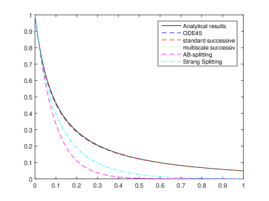
Figure 1: The solutions of the Bernoulli’s equation solved with the different splitting schemes.

Remark 4.1.

We compare the different standard splitting scheme, e.g., A-B splitting, Strang-splitting and the standard successive approximation based on a Bernoulli’s equation with a moderate nonlinearity. We obtain the best results in the case of the novel multiscale successive approximation method, while we include a more accurate resolution of the fast scales. We also obtain an fast method, that is competitive with the simple AB-splitting scheme. Such we improve the results with a more adapted novel scheme.

4.2 Second test example: Diffusion-Reaction equation with nonlinear reaction (Fisher’s equation)

We deal with the Fisher Equation, which describe the spreading of genes see [5] and has found applications in different fields of research ranging from ecology [9] to plasma physics [7].

We deal with a nonlinear PDE and split it into linear and nonlinear operators, while we can compare to a analytical solution.

The Fisher’s equation is given as

$$\frac{\partial u(x,t)}{\partial t} = D\partial_{xx}u+r(1-\frac{u}{K})u\;,\;\mbox{in}\;(x,t)\in\Omega\times[0,T]$$ (57)

$$u(x,0) = g(x)\;\mbox{on}\;x\in\Omega_{init},$$ (58)

$$u(x,t) = u_{analyt}(x,t)\;,\;\mbox{on}\;(x,t)\in\partial\Omega\times[0,T],$$ (59)

where we assume $\Omega\subset{\rm I}\!{\rm R}$. $u$ is the solution function, the initial condition is $g(x)$. Form the dynamical view-point, we apply a homogeneous medium with $D$ as diffusion coefficient and we embed a growth of a logistic function, see [10] with the $r$ is the growth rate and $K$ is the carrying capacity.

The analytical solution is given as:

$$u_{analyt}(x,t)=\frac{\exp(r\;t)}{1+\frac{1}{K}\left(\exp(r\;t)\tilde{u}(x,t)-g(x)\right)}\tilde{u}(x,t)\;.$$ (60)

where $\tilde{u}(x,t)=\frac{1}{\sqrt{1+4D\;t}}\int_{-\infty}^{\infty}\exp(-\frac{(x-\sigma)^{2}}{1+4D\;t})\;g(\sigma)\;d\sigma$.

and we apply the case $g(x)=\exp(-x^{2})$ and we have
$\tilde{u}(x,t)=\frac{1}{\sqrt{1+4D\;t}}\exp(-\frac{x^{2}}{1+4D\;t})$.

We rewrite the equation-system (68) in operator notation, and obtain the following equations :

$$\partial_{t}u = Au+B(u)u\;,$$ (61)

$$u(0) = u_{0},$$ (62)

and we split our operators to a linear and nonlinear one:

$$A=D\partial_{xx}+r$$ (63)

$$B(u)=-r\frac{u}{K},$$ (64)

with $D=0.01,\;r=1,K=1$, later we apply the multiscale case with $K=0.5,0.25$.

• Analytical Solution of the Diffusion-Reaction Part:
  Based on the one-dimensional problem, we can apply the analytical solution of the diffusion-convection part means:

  $$\frac{\partial u(x,t)}{\partial t} = D\partial_{xx}u+ru\;,\;\mbox{in}\;(x,t)\in\Omega\times[0,T]$$ (65)

  $$u(x,0) = u_{0}(x)\;\mbox{on}\;x\in\Omega_{init},$$ (66)

  $$u(x,t) = u_{analyt}(x,t)\;,\;\mbox{on}\;(x,t)\in\partial\Omega\times[0,T],$$ (67)

  where we assume $\Omega\subset{\rm I}\!{\rm R}$. $u$ is the solution function, the initial condition is $u_{0}(x)$. Further $D$ is the diffusion coefficient and $r$ the growth rate.

  The analytical solution is given as:

  $$u_{analyt}(x,t)=\exp(r\;t)\tilde{u}(x,t)\;.$$ (68)

  where $\tilde{u}(x,t)=\frac{1}{\sqrt{1+4D\;t}}\int_{-\infty}^{\infty}\exp(-\frac{(x-\sigma)^{2}}{1+4D\;t})\;u_{0}(\sigma)\;d\sigma$.

• Numerical Solution of the Diffusion part:
  

  The operator $A$ is discretized as:

  $$A = \frac{D}{\Delta x^{2}}\cdot\left(\begin{array}[]{rrrrr}-2&1&{}\hfil&{}\hfil&{}\hfil\\ 1&-2&1&{}\hfil&{}\hfil\\ {}\hfil&\ddots&\ddots&\ddots&{}\hfil\\ {}\hfil&{}\hfil&1&-2&1\\ {}\hfil&{}\hfil&{}\hfil&1&-2\end{array}\right)$$ (74)

  $$+ r\left(\begin{array}[]{rrrrr}1&0&{}\hfil&{}\hfil&{}\hfil\\ 0&1&{}\hfil&{}\hfil&{}\hfil\\ {}\hfil&\ddots&\ddots&{}\hfil&{}\hfil\\ {}\hfil&{}\hfil&0&1&0\\ {}\hfil&{}\hfil&{}\hfil&0&1\end{array}\right)~{}\in~{}{\rm I}\!{\rm R}^{I\times I},$$ (80)

  where $I$ are the number of discretization points, e.g. $I=100$.

  The operator $B$ is written in the operator notation as:

  $$B(u)=-\frac{r}{K}\left(\begin{array}[]{rrrrr}u_{1}(t)&0&{}\hfil&{}\hfil&{}\hfil\\ 0&u_{2}(t)&{}\hfil&{}\hfil&{}\hfil\\ {}\hfil&\ddots&\ddots&{}\hfil&{}\hfil\\ {}\hfil&{}\hfil&0&u_{I-1}(t)&0\\ {}\hfil&{}\hfil&{}\hfil&0&u_{I}(t)\end{array}\right)~{}\in~{}{\rm I}\!{\rm R}^{I\times I},$$ (86)

  where $I$ are the number of discretization points, e.g. $I=100$.

  The solution is given as ${\bf u}(t)=(u_{1}(t),\ldots,u_{I}(t))$, where $u_{i}(t)=u(x_{i},t),x_{i}=\Delta x\;i,\;i=1,\ldots,I$.

  Now, we can apply the discretized operator equations

  $$\frac{\partial{\bf u}(t)}{\partial t} = A{\bf u}+B({\bf u}){\bf u}\;,\;\mbox{in}\;t\in[0,T]$$ (87)

  $${\bf u}(0) = (g(x_{1}),\ldots,g(x_{I}))^{t},$$ (88)

  to our schemes.

The nonlinear behaves in a non-commutative manner $A^{\prime}B-B^{\prime}A\neq 0$.

We apply finite differences or finite elements to the spatial operator. With $\Omega=[0,10]$, $\Delta x=0.05$

We have the following results:

The results of the different schemes are shown in Figure 2.

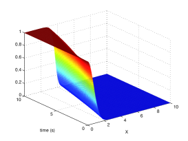
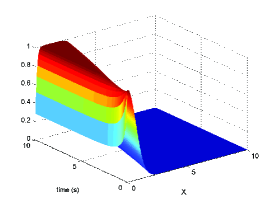
Figure 2: The solutions of the 1D Fisher’s equation with the analytical and numerical splitting schemes.

We have the following error in an $L_{2}$ Banach space:

$$E_{L_{2,\Delta x}}(t) = \sqrt{\int_{\Omega_{h}}(u_{ana}(x,t)-u_{num}(x,t))^{2}\;dx}$$ (89)

$$= \sqrt{\Delta x\sum_{i=1}^{N}(u_{ana}(x_{i},t)-u_{num}(x_{i},t))^{2}}$$ (90)

The results of the different schemes are shown in Figure 3.

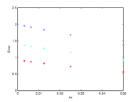
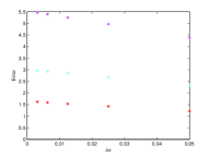
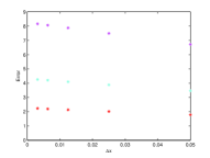
Figure 3: The solutions of the 1D Fisher’s equation with the numerical splitting schemes for $K=1,\;0.5,\;\mbox{and}\;0.25$ (asterisks in magenta $K=1.0$, cyan $K=0.5$ and red $K=0.25$), (left figure: $T=1$, middle figure: $T=5$ and right figure: $T=10$).

The results of the different norms are shown in Figure 4.

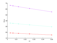
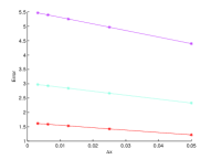
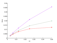
Figure 4: The solutions of the 1D Fisher’s equation with the numerical splitting schemes for $K=1,\;0.5,\;\mbox{and}\;0.25$ (asterisks in magenta $K=1.0$, cyan $K=0.5$ and red $K=0.25$), (left figure: $L_{1}$-norm, middle figure: $L_{2}$-norm and right figure: $L_{\infty}$-norm.

Remark 4.2.

We see the different solutions of the analytical and numerical solutions. The numerical solutions fit to the analytical solutions. The nonlinearity is optimal resolved and more effective with the successive approximation method. Their resolution over the different time-dependent terms is more resolved as for Magnus-expansion, which only average their nonlinear properties.

4.3 Third Example: 2d Fisher’s equation

We deal with the 2D Fisher Equation, which describe the spreading of genes see [5] and has found applications in different fields of research ranging from ecology [9] to plasma physics [7].

We deal with a nonlinear PDE and split it into linear and nonlinear operators, while we can compare to a analytical solution.

The Fisher’s equation is given as

$$\frac{\partial u(x,y,t)}{\partial t} = D_{x}\partial_{xx}u+D_{y}\partial_{yy}u+r(1-\frac{u}{K})u\;,\;\mbox{in}\;(x,t)\in\Omega\times[0,T],$$ (91)

$$u(x,y,0) = g(x,y)\;,\;\mbox{on}\;(x,y)\in\Omega,$$ (92)

$$u(x,y,t) = 0\;,\;\mbox{on}\;(x,y,t)\in\partial\Omega\times[0,T],$$ (93)

where we assume $\Omega=[-2,2]\times[-2,2]\subset{\rm I}\!{\rm R}^{2}$, such that we could apply the Dirichlet-boundary conditions $u(x,y,t)=0,\;\partial\Omega\times[0,T]$. $u$ is the solution function, the initial condition is $g(x,y)$. Form the dynamical view-point, we apply a homogeneous medium with $D$ as diffusion coefficient and we embed a growth of a logistic function, see [10] with the $r$ is the growth rate and $K$ is the carrying capacity.

We apply the case $g(x,y)=\exp(-x^{2}-y^{2})$ .

We rewrite the equation-system (68) in operator notation, and obtain the following equations :

$$\partial_{t}u = Au+B(u)u\;,$$ (94)

$$u(0) = u_{0},$$ (95)

and we split our operators to a linear and nonlinear one:

$$A=D_{x}\partial_{xx}+D_{y}\partial_{yy}+r$$ (96)

$$B(u)=-r\frac{u}{K},$$ (97)

with $D_{x}=D_{y}=0.01,\;r=1,K=1$, later we apply the multiscale case with $K=0.5,0.25$.

Numerical Solution of the Diffusion part:

The operator $A$ is discretized as:

$$A = \frac{D}{\Delta x^{2}}\cdot\left(\begin{array}[]{rrrrr}-T&I&{}\hfil&{}\hfil&{}\hfil\\ I&-T&I&{}\hfil&{}\hfil\\ {}\hfil&\ddots&\ddots&\ddots&{}\hfil\\ {}\hfil&{}\hfil&I&-T&I\\ {}\hfil&{}\hfil&{}\hfil&I&-T\end{array}\right)$$ (103)

$$+ r\left(\begin{array}[]{rrrrr}1&0&{}\hfil&{}\hfil&{}\hfil\\ 0&1&{}\hfil&{}\hfil&{}\hfil\\ {}\hfil&\ddots&\ddots&{}\hfil&{}\hfil\\ {}\hfil&{}\hfil&0&1&0\\ {}\hfil&{}\hfil&{}\hfil&0&1\end{array}\right)~{}\in~{}{\rm I}\!{\rm R}^{I^{2}\times I^{2}},$$ (109)

$$T = \left(\begin{array}[]{rrrrr}4&-1&{}\hfil&{}\hfil&{}\hfil\\ -1&4&-1&{}\hfil&{}\hfil\\ {}\hfil&\ddots&\ddots&\ddots&{}\hfil\\ {}\hfil&{}\hfil&-1&4&-1\\ {}\hfil&{}\hfil&{}\hfil&-1&4\end{array}\right)~{}\in~{}{\rm I}\!{\rm R}^{I\times I},$$ (115)

where $I$ are the number of discretization points, e.g. $I=100$.

The operator $B$ is written in the operator notation as:

$$B(u) = -\frac{r}{K}\left(\begin{array}[]{rrrrr}u_{1}(t)&0&{}\hfil&{}\hfil&{}\hfil\\ 0&u_{2}(t)&{}\hfil&{}\hfil&{}\hfil\\ {}\hfil&\ddots&\ddots&{}\hfil&{}\hfil\\ {}\hfil&{}\hfil&0&u_{I^{2}-1}(t)&0\\ {}\hfil&{}\hfil&{}\hfil&0&u_{I^{2}}(t)\end{array}\right)~{}\in~{}{\rm I}\!{\rm R}^{I^{2}\times I^{2}},$$ (121)

where $I$ are the number of discretization points, e.g. $I=100$.

The solution is given as ${\bf u}(t)=(u_{1}(t),\ldots,u_{I}(t),u_{I+1}(t),\ldots,u_{I^{2}}(t)$ . where $u_{i}(t)=u(x_{j},y_{k},t),x_{j}=\Delta x\;j,\;j=1,\ldots,I,\;y_{k}=\Delta x\;j,\;k=1,\ldots,I$ and $i=I(k-1)+j$.

Now, we can apply the discretized operator equations given in the following:

$$\frac{\partial{\bf u}(t)}{\partial t} = A{\bf u}+B({\bf u}){\bf u}\;,\;\mbox{in}\;t\in[0,T]$$ (122)

$${\bf u}(0) = (g(x_{1},y_{1}),\ldots,g(x_{I},y_{I}))^{t},$$ (123)

to our splitting schemes.

The nonlinear behaves in a non-commutative manner $A^{\prime}B-B^{\prime}A\neq 0$.

We apply finite differences or finite elements to the spatial operator. With $\Omega=[-2,2]\times[-2,2]$, $\Delta x=\Delta y=0.05$

We have the following results:

We have the following error in an $L_{\infty}$ Banach space:

$$E_{L_{\infty,\Delta x}}(t) = \sup\nolimits_{x\in\Omega_{h}}|u_{num,\Delta x/8}(x,t)-u_{num}(x,t)|$$ (124)

$$= \sup\nolimits_{i=1}^{N}|u_{num,\Delta x/8}(x_{i},t)-u_{num}(x_{i},t)|.$$

We have the following error in an $L_{1}$ Banach space:

$$E_{L_{1,\Delta x}}(t) = \int_{\Omega_{h}}|u_{num,\Delta x/8}(x,t)-u_{num}(x,t)|\;dx$$ (125)

$$= \Delta x\sum_{i=1}^{N}|u_{num,\Delta x/8}(x_{i},t)-u_{num}(x_{i},t)|.$$

We have the following error in an $L_{2}$ Banach space:

$$E_{L_{2,\Delta x}}(t) = \sqrt{\int_{\Omega_{h}}(u_{num,\Delta x/8}(x,t)-u_{num}(x,t))^{2}\;dx}$$ (126)

$$= \sqrt{\Delta x\sum_{i=1}^{N}(u_{num,\Delta x/8}(x_{i},t)-u_{num}(x_{i},t))^{2}}.$$

The results of the different schemes are shown in Figure 5.

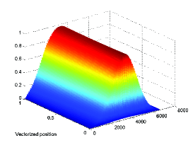
Figure 5: The solutions of the 2d Fisher’s equation of the numerical solution.

The convergence results of the different schemes are shown in Figure 6.

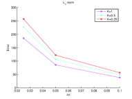
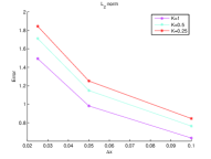
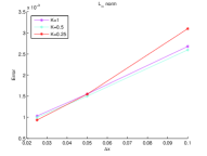
Figure 6: The convergence results of the 2d Fisher’s equation (left figure: $L_{1}$ error, middle figure: $L_{2}$ error, right figure: $L_{inf}$ errors).

Remark 4.3.

We see the different solutions of the analytical and numerical solutions. Here, we have a higher inverstigation to the spatial discretization and therefore also for the solvers. The numerical solutions fit to the analytical solutions. We have the same improvements also for the higher dimensions, that we resolved the nonlinear terms via Taylor-expension in the Multiscale method more accurate as with the Magnus-expansion.

4.4 Forth Example: 3d Fisher’s equation

We deal with the 3D Fisher Equation, which describe the spreading of genes see [5] and has found applications in different fields of research ranging from ecology [9] to plasma physics [7].

We deal with a nonlinear PDE and split it into linear and nonlinear operators, while we can compare to a analytical solution.

The Fisher’s equation is given as

$$\frac{\partial u(x,y,z,t)}{\partial t} = D_{x}\partial_{xx}u+D_{y}\partial_{yy}u+D_{z}\partial_{zz}u$$ (127)

$$+r(1-\frac{u}{K})u\;,\;\mbox{in}\;(x,t)\in\Omega\times[0,T],$$

$$u(x,y,z,0) = g(x,y,z)\;,\;\mbox{on}\;(x,y)\in\Omega,$$ (128)

$$u(x,y,z,t) = 0\;,\;\mbox{on}\;(x,y,z,t)\in\partial\Omega\times[0,T],$$ (129)

where we assume $\Omega=[-0.5,0.5]\times[-0.5,0.5]\times[-0.5,0.5]\subset{\rm I}\!{\rm R}^{3}$, such that we could apply the Dirichelt-boundary conditions $u(x,y,z,t)=0,\;\partial\Omega\times[0,T]$. $u$ is the solution function, the initial condition is $g(x,y,z)$. Form the dynamical view-point, we apply a homogeneous medium with $D$ as diffusion coefficient and we embed a growth of a logistic function, see [10] with the $r$ is the growth rate and $K$ is the carrying capacity.

We apply the case $g(x,y)=\exp(-x^{2}-y^{2}-z^{2})$ .

We rewrite the equation-system (68) in operator notation, and obtain the following equations :

$$\partial_{t}u = Au+B(u)u\;,$$ (130)

$$u(0) = u_{0},$$ (131)

and we split our operators to a linear and nonlinear one:

$$A=D_{x}\partial_{xx}+D_{y}\partial_{yy}+D_{zz}\partial_{zz}+r$$ (132)

$$B(u)=-r\frac{u}{K},$$ (133)

with $D_{x}=D_{y}=D_{z}=0.01,\;r=1,K=1$, later we apply the multiscale case with $K=0.5,0.25$.

Numerical Solution of the Diffusion part:

The operator $A$ is discretized as:

$$A = \frac{D}{\Delta x^{2}}\cdot\left(\begin{array}[]{rrrrr}T_{1}&I_{1}&&\ldots\\ I_{1}&T_{1}&I_{1}&{}\hfil&{}\hfil\\ {}\hfil&\ddots&\ddots&\ddots&{}\hfil\\ {}\hfil&{}\hfil&I_{1}&T_{1}&I_{1}\\ {}\hfil&{}\hfil&{}\hfil&I_{1}&T_{1}\end{array}\right)$$ (139)

$$+ r\left(\begin{array}[]{rrrrr}1&0&{}\hfil&{}\hfil&{}\hfil\\ 0&1&{}\hfil&{}\hfil&{}\hfil\\ {}\hfil&\ddots&\ddots&{}\hfil&{}\hfil\\ {}\hfil&{}\hfil&0&1&0\\ {}\hfil&{}\hfil&{}\hfil&0&1\end{array}\right)~{}\in~{}{\rm I}\!{\rm R}^{I^{3}\times I^{3}},$$ (145)

$$T_{1} = \left(\begin{array}[]{rrrrr}T&I&&\ldots\\ I&T&I&{}\hfil&{}\hfil\\ {}\hfil&\ddots&\ddots&\ddots&{}\hfil\\ {}\hfil&{}\hfil&I&T&I\\ {}\hfil&{}\hfil&{}\hfil&I&T\end{array}\right)~{}\in~{}{\rm I}\!{\rm R}^{I^{2}\times I^{2}},$$ (151)

$$I_{1} = \left(\begin{array}[]{rrrrr}I&0&&\ldots\\ 0&I&0&{}\hfil&{}\hfil\\ {}\hfil&\ddots&\ddots&\ddots&{}\hfil\\ {}\hfil&{}\hfil&=&I&0\\ {}\hfil&{}\hfil&{}\hfil&0&I\end{array}\right)~{}\in~{}{\rm I}\!{\rm R}^{I^{2}\times I^{2}},$$ (157)

$$T = \left(\begin{array}[]{rrrrr}-6&1&{}\hfil&{}\hfil&{}\hfil\\ 1&-6&1&{}\hfil&{}\hfil\\ {}\hfil&\ddots&\ddots&\ddots&{}\hfil\\ {}\hfil&{}\hfil&1&-6&1\\ {}\hfil&{}\hfil&{}\hfil&1&-6\end{array}\right)~{}\in~{}{\rm I}\!{\rm R}^{I\times I},$$ (163)

$$I = \left(\begin{array}[]{rrrrr}1&0&{}\hfil&{}\hfil&{}\hfil\\ 0&1&0&{}\hfil&{}\hfil\\ {}\hfil&\ddots&\ddots&\ddots&{}\hfil\\ {}\hfil&{}\hfil&0&1&0\\ {}\hfil&{}\hfil&{}\hfil&0&1\end{array}\right)~{}\in~{}{\rm I}\!{\rm R}^{I\times I},$$ (169)

where $I$ are the number of discretization points, e.g. $I=100$.

The operator $B$ is written in the operator notation as:

$$B(u)=-\frac{r}{K}\left(\begin{array}[]{rrrrr}u_{1}(t)&0&{}\hfil&{}\hfil&{}\hfil\\ 0&u_{2}(t)&{}\hfil&{}\hfil&{}\hfil\\ {}\hfil&\ddots&\ddots&{}\hfil&{}\hfil\\ {}\hfil&{}\hfil&0&u_{I^{3}-1}(t)&0\\ {}\hfil&{}\hfil&{}\hfil&0&u_{I^{3}}(t)\end{array}\right)~{}\in~{}{\rm I}\!{\rm R}^{I^{3}\times I^{3}},$$ (175)

where $I$ are the number of discretization points, e.g. $I=100$.

The solution is given as ${\bf u}(t)=(u_{1}(t),\ldots,u_{I}(t),u_{I+1}(t),\ldots,u_{I^{3}}(t)$ . where $u_{i}(t)=u(x_{j},y_{k},z_{l},t),x_{j}=\Delta x\;j,\;j=1,\ldots,I,\;y_{k}=\Delta x\;j,\;k=1,\ldots,I\;y_{l}=\Delta x\;l,\;l=1,\ldots,I$ and $i=I^{2}(l-1)+I(k-1)+j$.

Now, we can apply the discretized operator equations to our splitting schemes, which are given as:

$$\frac{\partial{\bf u}(t)}{\partial t} = A{\bf u}+B({\bf u}){\bf u}\;,\;\mbox{in}\;t\in[0,T]$$ (176)

$${\bf u}(0) = (g(x_{1},y_{1},z_{1}),\ldots,g(x_{I},y_{I},z_{I}))^{t}.$$ (177)

The nonlinear behaves in a non-commutative manner $A^{\prime}B-B^{\prime}A\neq 0$.

We apply finite differences or finite elements to the spatial operator. With $\Omega=[-0.5,0.5]\times[-0.5,0.5]\times[-0.5,0.5],\Delta x=\Delta y=\Delta z=0.05$.

We have the following results:

We have the following relative error in an $L_{\infty}$ Banach space:

$$E_{L_{\infty,\Delta x},rel}(t) = \frac{\sup\nolimits_{x\in\Omega_{h}}|u_{num,\Delta x/8}(x,t)-u_{num}(x,t)|}{\sup\nolimits_{x\in\Omega_{h}}|u_{num,\Delta x/8}(x,t)|}$$ (178)

$$= \frac{\sup\nolimits_{i=1}^{N}|u_{num,\Delta x/8}(x_{i},t)-u_{num}(x_{i},t)|}{\sup\nolimits_{i=1}^{N}|u_{num,\Delta x/8}(x_{i},t)|}.$$

We have the following error in an $L_{1}$ Banach space:

$$E_{L_{1,\Delta x},rel}(t) = \frac{\int_{\Omega_{h}}|u_{num,\Delta x/8}(x,t)-u_{num}(x,t)|\;dx}{\int_{\Omega_{h}}|u_{num,\Delta x/8}(x,t)|\;dx}$$ (179)

$$= \frac{\Delta x\sum_{i=1}^{N}|u_{num,\Delta x/8}(x_{i},t)-u_{num}(x_{i},t)|}{\Delta x\sum_{i=1}^{N}|u_{num,\Delta x/8}(x_{i},t)|}.$$

We have the following error in an $L_{2}$ Banach space:

$$E_{L_{2,\Delta x,rel}}(t) = \frac{\sqrt{\int_{\Omega_{h}}(u_{num,\Delta x/8}(x,t)-u_{num}(x,t))^{2}\;dx}}{\sqrt{\int_{\Omega_{h}}(u_{num,\Delta x/8}(x,t))^{2}\;dx}}$$ (180)

$$= \frac{\sqrt{\Delta x\sum_{i=1}^{N}(u_{num,\Delta x/8}(x_{i},t)-u_{num}(x_{i},t))^{2}}}{\sqrt{\Delta x\sum_{i=1}^{N}(u_{num,\Delta x/8}(x_{i},t)}}.$$

The convergence results of the different schemes are shown in Figure 7.

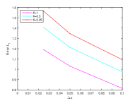
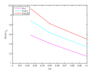
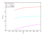
Figure 7: The convergence results of the 3d Fisher’s equation (left figure: $L_{1}$ relative error, middle figure: $L_{2}$ relative error, right figure: $L_{inf}$ relative errors).

Remark 4.4.

We see the different solutions of the analytical and numerical solutions. Here, we have a higher investigation to the spatial discretization and apply a fast computation via Leja-point of the $exp$-matrices, see [3]. The numerical solutions fit to the analytical solutions. We have the same improvements also for the higher dimensions, here we also resolve the nonlinear terms more accurate as with the Magnus-expansion.

5 Conclusions and Discussions

In this work, we have presented application to successive approximations that are related to iterative splitting schemes. We present the convergence analysis of the scheme and approximation to multiple scale methods. We see the benefits in resolving the nonlinearity in the Taylor-expension, such that we could conclude a higher order approximation of the nonlinearity in the recent time-step. Numerical experiments present the benefit of the scheme to standard Magnus expension methods. In future, we analyse and apply our method to different real-life applications.

References

- [1] S. Blanes and F. Casas. Splitting Methods for Non-autonomous separable dynamical systems. Journal of Physics A: Math. Gen., 39, 5405–5423, 2006.
- [2] S. Blanes, F. Casas, J.A. Oteo and J. Ros. The Magnus expansion and some of its applications. arXiv.org:0810.5488 (2008).
- [3] M. Caliari, P. Kandolf, A. Ostermann, and St. Rainer. Comparison of software for computing the action of the matrix exponential. BIT Numerical Mathematics, 54(1):113-128, 2014.
- [4] Casas, F., and A. Iserles. Explicit Magnus expansions for nonlinear equations. J. Phys. A: Math. Gen., 39, 5445–5461, 2006.
- [5] R.A. Fisher. The Wave of Advance of Advantageous Genes. Annals of Genetics, 7(4):353-369, 1937.
- [6] J. Geiser. Higher order splitting methods for differential equations: Theory and applications of a fourth order method. Numerical Mathematics: Theory, Methods and Applications. Global Science Press, Hong Kong, China, accepted, April 2008.
- [7] B.H. Gilding and R. Kersner. Travelling Waves in Nonlinear Diffusion Convection Reaction. Birkhäuser, Basel, 2004.
- [8] T. Jahnke and C. Lubich. Error bounds for exponential operator splittings. BIT Numerical Mathematics, 40:4, 735–745 (2000).
- [9] A. Kolmogorov, I. Petrovskii and N. Piscounov. Etude de L’equation de la Diffusion Avec Croissance de la Quan- tité de Matiere et Son Application a un Problem Biologique. In: V. M. Tikhomirov, Ed., Selected Works of A. Kolmogorov, Kluwer, Dordrecht, p. 248, 1991.
- [10] J. Vandermeer. How Populations Grow: The Exponential and Logistic Equations. Nature Education Knowledge, 3(10):15, 2010.
- [11] M. Suzuki. General Decomposition Theory of Ordered Exponentials. Proc. Japan Acad., vol. 69, Ser. B, 161 (1993).