Long-range spin and charge accumulation in mesoscopic superconductors with Zeeman splitting

Abstract

We describe the far from equilibrium non-local transport in a diffusive superconducting wire with a Zeeman splitting, taking into account the different spin relaxation mechanisms. We demonstrate that due to the Zeeman splitting an injection of a current in a superconducting wire creates a spin accumulation that can only relax via thermalization. In addition the Zeeman splitting also causes a suppression of the spin-orbit and spin-flip scattering rates. These two effects lead to long-range spin and charge accumulations detectable in the non-local signal. Our model explains the main qualitative features of recent experimental results in terms of realistic parameters and predicts a strong dependence of the non-local signal on the orbital depairing effect from an induced magnetic field.

Hybrid ferromagnetic/superconducting (FS) structures reveal a rich physics originating from the interplay between magnetism and superconductivity BuzdinRMP ; Bergeret2001 . While most of the research activity has been focused on the study and detection of proximity induced triplet superconducting correlations in an equilibrium situation Bergeret2001 ; triplet , more recent experiments addressed the problem of spin and charge accumulation in superconducting wiresFukuma2011 ; HanleSuper ; Poli ; SpinInjectionNb ; Aprili2013 ; Beckman2012 ; Beckman2014 . Figure 1 shows a typical experimental setup, in which a spin accumulation is generated by a spin-polarized current injected from a ferromagnetic electrode. This spin accumulation observed in the experiments can be quite large. Two puzzling findings motivate this Letter: First, in superconductors with a strong Zeeman splitting, the induced spin accumulation has been detected at distances from the injector much larger than the spin-relaxation length in the normal state Aprili2013 ; Beckman2012 ; Beckman2014 . Second, the non-local conductance $g_{nl}$ depends drastically on the origin of the Zeeman splitting. Such a splitting can be caused either by an applied (strong) external magnetic field Aprili2013 ; Beckman2012 or by the proximity of a ferromagnetic insulator Beckman2014proximity .

In this Letter, we develop a microscopic model based on the well-established Keldysh kinetic equations for superconductors extended to spin-dependent phenomena, and solve this puzzle. In particular we show that: (i) The observed long-range spin accumulation can be understood as a thermoelectric effect for Bogoliubov quasiparticles. The heating of a superconducting wire, originated for example from an injected current, produces a spin accumulation which can be detected as an electric signal by a spin-filter detector. The spin accumulation created in such a way can relax only due to the thermalization of injected quasiparticles and therefore the spin relaxation length is determined by inelastic electron-phonon and electron-electron scattering that can well exceed the usual spin diffusion length. (ii) Besides generating a large thermoelectric effect the Zeeman splitting also suppresses the spin-flip and spin-orbital scattering which are the main sources of charge imbalance relaxation in superconductors at low temperatures PairBreakingChImb . Hence the different behaviors observed for the non-local conductance $g_{nl}$ as a function of the injection voltage $V_{inj}$, depend on the value of the orbital depairing parameter $\alpha_{orb}$ defined below. For large enough values of $\alpha_{orb}$, at large applied fields the contribution from the charge imbalance to the non-local conductance is suppressed and the $g_{nl}(V_{inj})$ dependence is almost antisymmetric with respect to $V_{inj}$ Aprili2013 ; Beckman2012 ; Beckman2014 . In contrast, if the Zeeman splitting is caused by the proximity of a ferromagnetic insulator Beckman2014proximity , $\alpha_{orb}$ is small and the charge imbalance contribution to $g_{nl}$ becomes important. In this case, we predict a qualitative change of the non-local conductance as function of the injected current, that can be experimentally proven.

We consider the nonlocal spin valve shown in Fig. 1. A spin-polarized current is injected in the superconducting wire from a ferromagnetic electrode with polarization ${\bm{P}_{inj}}$, pointing in the direction of the magnetization. The detector is also a ferromagnet with a polarization vector ${\bm{P}_{det}}$ and located at a distance $L_{det}$ from the injector. Both the injector and the detector are coupled to the wire via tunnel contacts. A magnetic field ${\bm{B}}$ is applied in $z$ direction.

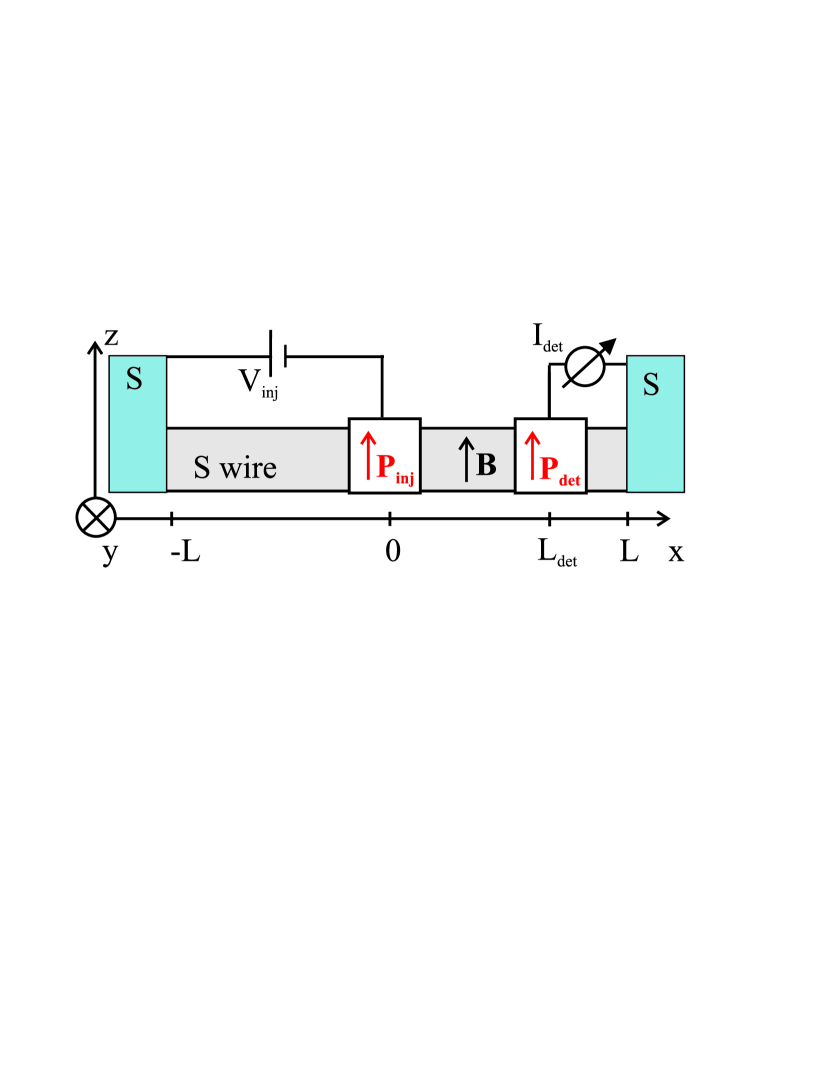
Figure 1: (Color online) Schematic view of the setup for nonlocal conductance measurements. Here we assume that the polarizations of the magnetic contacts are collinear to the magnetic field, ${\bm{P}_{inj}}\parallel{\bm{P}_{det}}\parallel{\bm{B}}$.

When ${\bm{P}_{inj}}\parallel{\bm{B}}\parallel{\bm{P}_{det}}$ (for the non-collinear case, see Ref. silaevup14 ), the tunnelling current at the detector is given by

$$R_{det}I_{det}=\mu+P_{det}\mu_{z}$$ (1)

where $R_{det}$ is the detector interface resistance in the normal state, $\mu$ is the charge imbalance and $\mu_{z}$ the spin imbalance. Here we assume that the detector current is measured at zero bias $V_{det}=0$. The nonlocal differential conductance measured in the experiment is $g_{nl}=dI_{det}/dV_{inj}$.

The charge imbalance $\mu$ and spin accumulation $\mu_{z}$ can be expressed in terms of the Keldysh quasiclassical Green function (GF) as $\mu=\int_{0}^{\infty}{\rm Tr}(g^{K})d\varepsilon/16$ and $\mu_{z}=\int_{0}^{\infty}{\rm Tr}[\tau_{3}\sigma_{3}(g^{K}-g^{K}_{eq})]d\varepsilon/16$. Here $\tau_{3}$ ($\sigma_{3}$) is the third Pauli matrix in Nambu (spin) space, $g^{K}$ is the (4$\times$4 matrix) Keldysh component of the quasiclassical GF matrix $\check{g}=\left(\begin{array}[]{cc}g^{R}&g^{K}\\ 0&g^{A}\\ \end{array}\right)$, and $g^{R(A)}$ is the retarded (advanced) GF. We denote $g^{K}_{eq}=g^{K}$ at the equilibrium state. The matrix GF satisfies the normalization condition $\check{g}^{2}=1$ that allows writing the Keldysh component as $g^{K}=g^{R}\hat{f}-\hat{f}g^{A}$, where $\hat{f}$ is the distribution function with a general spin structure $\hat{f}=f_{L}+f_{T}\tau_{3}+f_{T3}\sigma_{3}+f_{L3}\tau_{3}\sigma_{3}$SupplMat . With the help of the above notations we obtain the expressions for the charge and spin imbalance in the superconductor (here and below, $\hbar=k_{B}=1$)

$$\mu=\frac{1}{2}\int_{0}^{\infty}d\varepsilon(N_{+}f_{T}+N_{-}f_{L3})$$ (2)

$$\mu_{z}=\frac{1}{2}\int_{0}^{\infty}d\varepsilon[N_{+}f_{T3}+N_{-}(f_{L}-n_{0})],$$ (3)

where $N_{+}$ is the total density of states (DOS), $N_{-}$ is the DOS difference between the spin subbands, and $n_{0}(\varepsilon)=\tanh(\varepsilon/2T)$.

According to Eq. (3) there are two contributions to the spin signal. One is generated from the longitudinal component $f_{L}$. This contribution is only finite in the presence of a Zeeman splitting of the DOS ($N_{-}\neq 0$). The second contribution is described by the first term in the integrand of Eq. (3) and it is finite even in the absence of an exchange field. While this latter contribution has been analyzed in Ref. Beckman2012 , we show below that in several cases it is the longitudinal contribution that dominates the spin signal due to its long-range character.

In order to obtain the kinetic equations in a diffusive spin-polarized superconductor we start from the general Usadel equation Bergeret2001

$$D\nabla\cdot(\check{g}\nabla\check{g})+[\check{\Lambda}-\check{\Sigma}_{so}-\check{\Sigma}_{sf}-\check{\Sigma}_{orb},\check{g}]=0.$$ (4)

Here $D$ is the diffusion constant, $\check{\Lambda}=i\varepsilon\tau_{3}-i({\bm{h\cdot S})}\tau_{3}-\check{\Delta}$, $\varepsilon$ is the energy, $\check{\Delta}=\Delta\tau_{1}$ the spatially homogeneous order parameter in the wire, ${\bm{h}}$ is the Zeeman field, and ${\bm{S}}=(\sigma_{1},\sigma_{2},\sigma_{3})$ the vector of Pauli matrices in spin space. The last three terms in Eq. (4), $\check{\Sigma}_{so}=\tau_{so}^{-1}({\bm{S}}\cdot\check{g}{\bm{S}})$, $\check{\Sigma}_{sf}=\tau_{sf}^{-1}({\bm{S}}\cdot\tau_{3}\check{g}\tau_{3}{\bm{S}})$ and $\check{\Sigma}_{orb}=\tau_{orb}^{-1}\tau_{3}\check{g}\tau_{3}$ describe spin and charge imbalance relaxation due to the spin-orbit scattering, exchange interaction with magnetic impurities and orbital magnetic depairing, characterized by the relaxation times $\tau_{so}$, $\tau_{sf}$ and $\tau_{orb}$, respectively.

The orbital depairing rate can be written in the form $\tau^{-1}_{orb}=T_{c}\alpha_{orb}(h/T_{c})^{2}$ where $\alpha_{orb}$ is the dimensionless parameter measuring the relative strength of orbital and paramagnetic effects and $T_{c}$ is the critical temperature of the superconductor for $h=0$. If the Zeeman field is provided by an external magnetic field Beckman2012 ; Aprili2013 ${\bm{h}}=\mu_{B}{\bm{B}}$ where $\mu_{B}$ is the Bohr magneton then $\alpha_{orb}=T_{c}\Delta/(\mu^{2}_{B}B^{2}_{c})$, where $B_{c}=\sqrt{12}\phi_{0}/(\pi\xi W)$ is the critical field of a thin superconducting film of width $W$, $\xi=\sqrt{D/\Delta}$ is the superconducting coherence length and $\phi_{0}=h/(2e)$ is the magnetic flux quantum SchmidtDepairing . Assuming $\Delta=240$ $\mu$eV and diffusion constant $D=40$ cm²/s Beckman2012 ; Beckman2014 , we obtain $\alpha_{orb}\approx 210(W/\xi)^{2}$ where $\xi\approx 100$ nm. This estimation yields $\alpha_{orb}=1.33$ for the film width $W=8$ nm. The Zeeman field can also be induced by an exchange field in a FS proximity system Beckman2014proximity . In this case $\tau_{orb}$ is not directly related to the Zeeman field and we describe this with $\alpha_{orb}=0$ in the numerical results below.

We assume that the transparencies of the detector and injector interfaces are small, so that up to leading order the retarded and advanced GF are the bulk ones determined by the nonlinear equation $[\Lambda^{R}-\Sigma^{R}_{sf}-\Sigma^{R}_{so}-\Sigma^{R}_{orb},g^{R}]=0$. In the presence of an exchange field ${\bm{h}}=h{\bm{z}}$, the spectral functions read $g^{R}=g_{01}\tau_{1}+g_{31}\sigma_{3}\tau_{1}+g_{03}\tau_{3}+g_{33}\sigma_{3}\tau_{3}$ and $g^{A}=-\tau_{3}g^{R{\dagger}}\tau_{3}$. While the terms diagonal in Nambu space ($\tau_{3}$) correspond to the normal GFs, the $g_{01},g_{31}$ describe the singlet and zero-spin triplet anomalous components Bergeret2001 . From these GFs we get $N_{+}={\rm Re}g_{03}$, $N_{-}={\rm Re}g_{33}$ in Eqs. (2,3).

From Eq. (4) we obtain two decoupled sets of kinetic equations complemented by boundary conditions (BC) at the spin-polarized injector interface $z=0$. We use the BC of Ref. bergeret12 that generalizes the Kupriyanov-Lukichev KL one to the case of spin-dependent barrier transmission.

We start analyzing the set of equations that couple the components $f_{T}$ and $f_{L3}$. These determine the charge ${\bm{j_{c}}}$ and spin-heat ${\bm{j_{se}}}$ currents according to:

$${\bm{j_{c}}}={\mathcal{D}}_{T}\nabla f_{T}+{\mathcal{D}}_{L3}\nabla f_{L3}$$ (5)

$${\bm{j_{se}}}={\mathcal{D}}_{T}\nabla f_{L3}+{\mathcal{D}}_{L3}\nabla f_{T},$$ (6)

where the diffusion coefficients are

$${\mathcal{D}}_{T} = D\left(1+|g_{01}|^{2}+|g_{03}|^{2}+|g_{31}|^{2}+|g_{33}|^{2}\right)$$ (7)

$${\mathcal{D}}_{L3} = 2D{\rm Re}\left(g_{03}g_{33}^{*}+g_{01}g_{31}^{*}\right).$$ (8)

These currents satisfy a pair of coupled diffusion equations

$${\bm{\nabla\cdot j_{c}}} = R_{T}f_{T}+R_{L3}f_{L3}$$ (9)

$${\bm{\nabla\cdot j_{se}}} = (R_{T}+S_{L3})f_{L3}+R_{L3}f_{T},$$ (10)

supplemented by the BC at the injector electrode $x=0$:

$${\bm{j_{c}}}=\frac{\kappa_{I}}{D}\{N_{+}(f_{T}-n_{-})+N_{-}[P_{I}(n_{0}-n_{+})+f_{L3}]\}$$

$${\bm{j_{se}}}=\frac{\kappa_{I}}{D}\{N_{-}(f_{T}-n_{-})+N_{+}[P_{I}(n_{0}-n_{+})+f_{L3}]\},$$

where $n_{\pm}=[n_{0}(\varepsilon+V_{inj})\pm n_{0}(\varepsilon-V_{inj})]/2$. The coefficients in Eqs.  (9,10) are given by $R_{T}=4\Delta{\rm Re}g_{01}$, $R_{L3}=4\Delta{\rm Re}g_{31}$, and

$$S_{L3}=\frac{16}{\tau_{\Sigma}}\{({\rm Re}g_{03})^{2}-({\rm Re}g_{33})^{2}+\beta\left[({\rm Re}g_{31})^{2}-({\rm Re}g_{01})^{2}\right]\}.$$

Here $\tau^{-1}_{\Sigma}=\tau^{-1}_{so}+\tau^{-1}_{sf}$ and the parameter $\beta=(\tau_{so}-\tau_{sf})/(\tau_{so}+\tau_{sf})$ characterizes the relative strength of spin-orbit and spin-flip scattering. For example, in Al wires used in the spin-transport experiments, the typical spin relaxation time is $\tau_{\Sigma}\approx 800$ ps $\approx 40/T_{c}$ where $T_{c}\approx 1.6$ K. For the spin accumulation experiments Beckman2012 ; Beckman2014 ; Beckman2014proximity the value of $\beta$ can be inferred from the magnetic depairing parameter $\zeta=8\cdot 10^{-4}$ in the absence of a magnetic field. It is proportional to the spin-flip scattering rate $\zeta=3(1+\beta)/(2\tau_{\Sigma}T_{c})$ which yields $\beta\approx-0.98$. We use $\beta=-0.9$ to obtain the qualitative effects.

The solution of the system (9,10) is given by the superposition of two exponentially decaying functions $e^{-k_{T1,2}x}$ with amplitudes determined by the BC. The energy dependencies of $k_{T1,2}$ are shown in Fig. 2a,b for the cases of strong and weak orbital depairing. The charge and spin-heat imbalance relaxation is non-zero above the gap $k_{T1,2}\neq 0$ due to the magnetic pair breaking effects ShcmidSchoen1975 ; PairBreakingChImb .

The other set of equations are for the components $f_{L},f_{T3}$ that determine the energy and pure spin currents

$${\bm{j_{e}}}={\mathcal{D}}_{L}\nabla f_{L}+{\mathcal{D}}_{T3}\nabla f_{T3}$$ (11)

$${\bm{j_{s}}}={\mathcal{D}}_{L}\nabla f_{T3}+{\mathcal{D}}_{T3}\nabla f_{L}$$ (12)

satisfying the diffusion equations

$${\bm{\nabla\cdot j_{e}}} = 0$$ (13)

$${\bm{\nabla\cdot j_{s}}} = S_{T3}f_{T3},$$ (14)

where the diffusion coefficients are

$${\mathcal{D}}_{L} = D\left(1-|g_{01}|^{2}+|g_{03}|^{2}-|g_{31}|^{2}+|g_{33}|^{2}\right)$$ (15)

$${\mathcal{D}}_{T3} = 2D{\rm Re}\left(g_{03}g_{33}^{*}-g_{01}g_{31}^{*}\right)$$ (16)

and

$$S_{T3}=\frac{16}{\tau_{\Sigma}}\{({\rm Re}g_{03})^{2}-({\rm Re}g_{33})^{2}+\beta\left[({\rm Im}g_{01})^{2}-({\rm Im}g_{31})^{2}\right]\}.$$

The boundary conditions at $x=0$ are

$${\bm{j_{e}}}=\frac{\kappa_{I}}{D}[N_{+}(f_{L}-n_{+})+N_{-}(f_{T3}-P_{I}n_{-})]$$ (17)

$${\bm{j_{s}}}=\frac{\kappa_{I}}{D}[N_{-}(f_{L}-n_{+})+N_{+}(f_{T3}-P_{I}n_{-})],$$ (18)

where $n_{\pm}=n_{\pm}(V_{inj})$.

The solution of the system (13,14) is given by a superposition of two qualitatively different terms

$$\left(f_{L}\atop f_{T3}\right)=A\left(1\atop-{\mathcal{D}}_{L}/{\mathcal{D}}_{T3}\right)e^{-k_{L}x}+\left(\alpha(x-L)\atop 0\right),$$ (19)

where the amplitudes $(\alpha,A)$ can be found from the BC (17,18). The first term in (19) describes a decay of the (spectral) spin imbalance with a characteristic length scale $k_{L}=\sqrt{S_{T3}{\mathcal{D}}_{L}/({\mathcal{D}}_{L}^{2}-{\mathcal{D}}_{T3}^{2})}$. The second term in (19) describes the rise of quasiparticle temperature generated by the applied voltage $V_{inj}$. This decays only via inelastic scattering disregarded in the above equations, but discussed in more detail below.

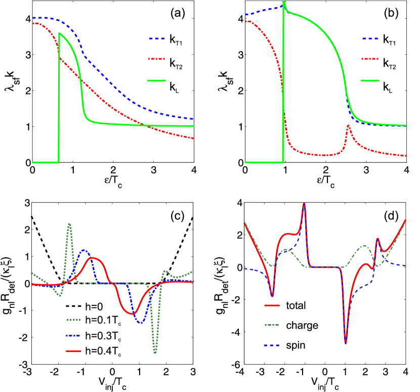
Figure 2: (Color online) (a,b) Energy dependence of the inverse length scales $k_{T1,2}$ and $k_{L}$ for: (a) $\alpha_{orb}=1.33$ and $h=0.3T_{c}$; (b) $\alpha_{orb}=0$, and $h=0.8T_{c}$ (here $\lambda_{sf}=\sqrt{D\tau_{\Sigma}/8}$ is the normal state spin relaxation length). Panels (c) and (d) show the nonlocal conductance as a function of the injecting voltage, $g_{nl}(V_{inj})$ for: (c) $\alpha_{orb}=1.33$ and $h=0;\;0.1;\;0.3;\;0.4T_{c}$. (d) $\alpha_{orb}=0$ and $h=\;0.8T_{c}$. Red solid line shows the total signal, blue dashed and green dash-dotted lines show the spin and charge imbalance contributions respectively. The parameters common to all panels are $T=0.05\;T_{c}$, $\beta=-0.9$, $\tau_{\Sigma}T_{c}=40$, $P_{inj}=-P_{det}=0.1$, $\kappa_{I}\xi=0.02$, the inelastic relaxation length $L=20\lambda_{sf}$ and $L_{det}=5\lambda_{sf}$.

We now calculate the non-local conductance from Eq. (1) and the solutions of kinetic equations (9,10,13,14). First, we assume a strong orbital depairing $\alpha_{orb}=1.33$. Figure (2)c shows the non-local conductance and describes several features observed in recent experiments Aprili2013 ; Beckman2012 ; Beckman2014 that we discuss below.

In the absence of a Zeeman field, $N_{-}=0$, and therefore only the first terms in the r.h.s of Eqs. (2-3) contributes to $g_{nl}$. For $h=0$ the contribution stemming from the spin accumulation is finite only if $P_{inj}\neq 0$, which is the condition to obtain a finite $f_{T3}$. However, this function decays over the short spin diffusion length and therefore is negligibly small at the distances $L_{det}=3\lambda_{sf}$ from the injector. Thus, the detected signal in this case is mostly determined by the charge imbalance, Eq. (2). This explains the symmetry with respect to the injecting voltage: $g_{nl}(V_{inj})=g_{nl}(-V_{inj})$. The charge imbalance contribution to $g_{nl}$ grows monotonically when $|V_{inj}|>\Delta_{g}$. This behavior is determined by the increase of the charge relaxation scale at large energies $k^{-1}_{T2}\rightarrow\infty$ shown in Fig. 2a.

In the presence of a magnetic field, on the one hand, the charge relaxation is strongly enhanced due to the orbital depairing effect. This explains a strong suppression of the charge imbalance background signal by increased $h$ in Fig. 2c. On the other hand the spin imbalance contribution stemming from the second term in the r.h.s of Eq. (3) is large. As shown above, this term describes the heat injection in the presence of a finite Zeeman field $h$ and has a long-range behavior. This contribution leads to the large peaks in $g_{nl}(V_{inj})$ shown in Fig. 2c. In contrast to the linear thermoelectric effect ThermoelectriEschrig ; ThermoelectriOsaeta , which is exponentially small for temperatures well below the energy gap $T\ll\Delta$, a non-linear heating produced by quasiparticles injected at voltages exceeding the energy gap explains the large electric signal observed in the experiments Aprili2013 ; Beckman2012 ; Beckman2014 . Notice that the peaks do not have exactly the same form so that $g_{nl}(V_{inj})\neq-g_{nl}(-V_{inj})$. The small deviation from the antisymmetric case is due to the small but finite injector polarization $P_{inj}$, as well as to the presence of an admixture of the charge imbalance signal.

Next let us consider the case of no orbital depairing $\alpha_{orb}=0$. This may correspond to the case of a Zeeman field caused by the proximity of a ferromagnetic insulator Beckman2014proximity . Figure 2d shows a clearly different behavior for $g_{nl}(V_{inj})$ with respect to the large $\alpha_{orb}$ case, and can be observed in the experiments Beckman2014proximity . Now the asymmetry of the $g_{nl}(V_{inj})$ curve is much more pronounced and the peaks are much broader. This occurs due to a significant admixture of the long-range charge imbalance contribution (blue dashed curves) with the spin imbalance one (green dash-dotted curve). While the latter is almost perfectly antisymmetric the former produces symmetric peaks of $g_{nl}(V_{inj})$ at voltages within the interval $\Delta-h<V_{inj}<\Delta+h$. These peaks appear due to the strong suppression of charge relaxation by the Zeeman splitting at the energy interval $\Delta-h<\varepsilon<\Delta+h$, in accordance to Fig. 2b.

Our results give a qualitative explanation of experiments with large magnetic fields [Fig. 2c]. Including an additional constant orbital depairing which can originate from the stray fields of ferromagnetic contacts Aprili2013 we are able to obtain accurate fits of the experimental curves shown in Fig.3a of Ref. Beckman2012 using realistic parameters. Notice that the decay of the component $f_{L}$, responsible for the long-range spin imbalance, is only limited by inelastic relaxation, which have not been taken into account in our kinetic equations. The observed relaxation length $\lambda\sim 1$ $\mu$m likely cannot be explained by electron-phonon scattering, which already in the normal state leads to a much larger value $\lambda_{ph}=\sqrt{\tau_{ph}D}\approx 20$ ${\rm\mu m}$Beckman2012 ; Beckman2014 . Electron-electron scattering on the other hand can redistribute the total energy in the electron system and damp nonequilibrium components of the signal. In order to obtain the observed relaxation length $\lambda_{ee}\sim 1$ $\mu$m one should assume that the e-e scattering time is $\tau_{ee}\sim 10^{-10}s$ which is significantly less than the known value in bulk dirty Al KlapwijkRelTime but can be achieved in low-dimensional samples KlapwijkRelTime2D . The e-e thermalization process as well as nonuniversal properties of the heat transport in real experimental setups could explain the suppression of the spin imbalance relaxation by the Zeeman field Beckman2012 ; Beckman2014 .

To conclude, we have developed a theoretical framework to study the transport properties of superconductors with a Zeeman splitting. We have demonstrated that the splitting field leads to a strong suppression of the relaxation of charge and spin imbalances created by the injected current. In particular, the long-range spin accumulation observed in recent experiments is shown to be a manifestation of a non-linear thermoelectric effect and it is only limited by the inelastic relaxation length which can be larger than the spin relaxation time in normal metals by several orders of magnitude. Our model gives a qualitative explanation for a wide range of experiments on SF nonlocal spin valves, and predicts a strong dependence of the non-local conductance on orbital depairing, characterized by $\alpha_{\rm orb}$. Besides explaining the properties of superconductor-ferromagnet structures, our theory may be straightforwardly extended for the general description of thermoelectric effects in far from equilibrium situations in terms of the well-established theory of non-equilibrium GFs.

We thank Detlef Beckmann for discussions. The work of T.T.H was supported by the Academy of Finland Center of Excellence program and the European Research Council (Grant No. 240362-Heattronics). P.V. acknowledges the Academy of Finland for financial support. The work of F.S.B. was supported by the Spanish Ministry of Economy and Competitiveness under Project No. FIS2011-28851-C02- 02 and the Basque Government under UPV/EHU Project No. IT-756-13.

I Supplementary Material

We express the charge density, spin density, energy density and spin energy density in terms of the Nambu-Keldysh Green’s function and show that in the presence of a spin-splitting field their parametrization differs from the usual case.

We wish to characterize the state of the electron system in the superconductor via different matrix elements of the Nambu-Keldysh Green’s function. We choose the Nambu vector to be of the form

$$\Psi=\begin{pmatrix}\psi_{\uparrow}({\mathbf{r}},t)&\psi_{\downarrow}({\mathbf{r}},t)&-\psi_{\downarrow}^{\dagger}({\mathbf{r}},t)&\psi_{\uparrow}^{\dagger}({\mathbf{r}},t)\end{pmatrix},$$ (20)

where $\psi_{\sigma}^{(\dagger)}({\mathbf{r}},t)$ annihilates (creates) an electron of spin $\sigma$ in position ${\mathbf{r}}$ at time $t$. The Keldysh Green’s function is written in terms of the Nambu vector as

$$G^{K}(1,1^{\prime})=-i\tau_{3}\langle[\Psi(1),\Psi^{\dagger}(1^{\prime})]\rangle,$$ (21)

where the argument $1$ refers to position and time ${\mathbf{r}}_{1}$, $t_{1}$. Up to a state independent factor, the charge density can then be written as

$$\rho(1)=-ie{\rm Tr}[G^{K}(1,1)]/4=-ie\int\frac{d{\mathbf{p}}}{(2\pi)^{3}}\int_{-\infty}^{\infty}\frac{d\epsilon}{2\pi}{\rm Tr}[G^{K}(\epsilon,{\mathbf{p}},{\mathbf{r}},t)]/4,$$ (22)

where the latter form is expressed in the Wigner representation. This is thus the particle density averaged over spin.

The spin density in direction $\hat{u}_{j}\in\{\hat{u}_{x},\hat{u}_{y},\hat{u}_{z}\}$ is obtained from

$$s_{j}(1)=-i{\rm Tr}[\tau_{3}\sigma_{j}G^{K}]/4=-i\int\frac{d{\mathbf{p}}}{(2\pi)^{3}}\int_{-\infty}^{\infty}\frac{d\epsilon}{2\pi}{\rm Tr}[\tau_{3}\sigma_{j}G^{K}(\epsilon,{\mathbf{p}},{\mathbf{r}},t)]/4,$$ (23)

where $\tau_{j}(\sigma_{j})$ is the $j$th Pauli spin matrix in Nambu (spin) space. The multiplication with $\tau_{3}$ takes care of the chosen order of spins in the Nambu vector. In order to characterize the non-equilibrium spin accumulation we introduce the difference between the total spin density and the one at the equilibrium state

$$s_{ej}(1)=-i\int\frac{d{\mathbf{p}}}{(2\pi)^{3}}\int_{-\infty}^{\infty}\frac{d\epsilon}{2\pi}{\rm Tr}\{\tau_{3}\sigma_{j}[G^{K}(\epsilon,{\mathbf{p}},{\mathbf{r}},t)-G^{K}_{eq}(\epsilon,{\mathbf{p}},{\mathbf{r}},t)]\}/4.$$ (24)

As shown in the main text of the paper the spin accumulation ${\bf s}_{ej}$ determines the tunnelling current at the spin-polarized detector electrode in the non-local measurement scheme.

The spin-averaged energy density involves a multiplication by the Nambu matrix $\tau_{3}$ to take care of the fact that whereas particles and holes contribute to the charge an opposite amount, they contribute an equal amount to the excitation energy. We thus can write in the Wigner representation the (internal) energy density

$$\epsilon({\mathbf{r}},t)=-ie\int\frac{d{\mathbf{p}}}{(2\pi)^{3}}\int_{-\infty}^{\infty}\frac{d\epsilon}{2\pi}\epsilon{\rm Tr}[\tau_{3}G^{K}(\epsilon,{\mathbf{p}},{\mathbf{r}},t)]/4.$$ (25)

In the limit of a large bandwidth this becomes very large, so it is convenient to describe only the excess energy density compared to some equilibrium value,

$$\epsilon_{e}({\mathbf{r}},t)=-ie\int\frac{d{\mathbf{p}}}{(2\pi)^{3}}\int_{-\infty}^{\infty}\frac{d\epsilon}{2\pi}\epsilon{\rm Tr}\{\tau_{3}[G^{K}(\epsilon,{\mathbf{p}},{\mathbf{r}},t)-G^{K}_{\rm eq}(\epsilon,{\mathbf{p}},{\mathbf{r}},t)]\}/4.$$ (26)

Similarly to the charge density, $\epsilon_{e}$ is a spin-averaged quantity. We can thus also define the energy density difference in the two spin ensembles by

$$\epsilon_{j}({\mathbf{r}},t)=-ie\int\frac{d{\mathbf{p}}}{(2\pi)^{3}}\int_{-\infty}^{\infty}\frac{d\epsilon}{2\pi}\{\epsilon{\rm Tr}[\sigma_{j}G^{K}(\epsilon,{\mathbf{p}},{\mathbf{r}},t)]\}/4.$$ (27)

In the absence of a ferromagnetic transition, the contribution to this quantity comes from the small energy region related to voltage or temperature, and therefore there is no need to remove the equilibrium value.

We now define the quasiclassical Keldysh Green’s function in the diffusive limit (and a spherical Fermi surface) via

$$g^{K}(1)=\frac{i}{\pi}\int\frac{d\hat{p}}{4\pi}\int d\xi G^{K}(\epsilon,\xi,\hat{p},{\mathbf{r}},t),$$ (28)

where ${\mathbf{p}}=p\hat{p}$ and $\xi=p^{2}/(2m)-\epsilon_{F}$, where $\epsilon_{F}$ is the Fermi energy. Employing charge neutrality (charge density vanishes on length scales that are large compared to the usually microscopic screening length) and including the non-quasiclassical corrections in the standard way RammerBook , the electrostatic potential (instead of the charge density that vanishes) can be written in terms of the quasiclassical Green’s function as

$$\mu(\vec{r},t)=-\frac{1}{16}\int_{-\infty}^{\infty}d\epsilon{\rm Tr}[g^{K}(\epsilon,\vec{r},t)].$$ (29)

In the absence of a ferromagnetic transition, the other expressions can be then straightforwardly written in terms of the quasiclassical Green’s function by using

$$\int\frac{d{\mathbf{p}}}{(2\pi)^{3}}=\int d\xi N(\xi)\int\frac{d\hat{p}}{4\pi}\approx N_{0}\int d\xi\int\frac{d\hat{p}}{4\pi},$$ (30)

where $N(\xi)$ is the density of states in the normal state, and we assume $N(\xi)\approx N_{0}$ for excitation energies close to the Fermi surface. We hence get

$$s_{ej}(1) =-N_{0}\int_{-\infty}^{\infty}d\epsilon{\rm Tr}\{\tau_{3}\sigma_{j}[g^{K}(\epsilon,{\mathbf{r}},t)-g^{K}_{eq}(\epsilon,{\mathbf{r}},t)]\}/8.$$ (31)

$$\epsilon_{e}(1) =-N_{0}\int_{-\infty}^{\infty}d\epsilon\epsilon{\rm Tr}\{\tau_{3}[g^{K}(\epsilon,{\mathbf{r}},t)-g_{\rm eq}^{K}(\epsilon,\mathbf{r},t)]\}/8.$$ (32)

$$\epsilon_{j}(1) =-N_{0}\int_{-\infty}^{\infty}d\epsilon{\rm Tr}[\sigma_{j}g^{K}(\epsilon,{\mathbf{r}},t)]/8.$$ (33)

The full quasiclassical Keldysh Green’s function

$$\check{g}=\begin{pmatrix}g^{R}&g^{K}\\ 0&g^{A}\end{pmatrix}$$ (34)

satisfies the normalization condition $\check{g}^{2}=1$. This allows parameterizing $g^{K}=g^{R}f-fg^{A}$, where in the spin-dependent case the distribution function $f$ is parameterized by eight functions,

$$f=f_{L}+f_{T}\tau_{3}+\sum_{j}(f_{Tj}\sigma_{j}+f_{Lj}\sigma_{j}\tau_{j}).$$ (35)

Here the L-labelled functions denote the (spin) energy degrees of freedom and are antisymmetric in energy with respect to the Fermi level $\varepsilon=0$ in the superconductor. The T-labelled functions are symmetric in energy and describe the charge/spin imbalance.

In the main text, we only concentrate on the case of collinear spin configurations, and thereby it is enough to choose one of the spin directions, say $j=3$. In this case the above expressions for the local potential, nonequilibrium spin density, energy density and spin energy density can be written as

$$\mu(\vec{r},t) =-\frac{1}{2}\int_{0}^{\infty}d\epsilon(N_{+}f_{T}+N_{-}f_{L3})$$ (36)

$$s_{e3}(\vec{r},t) =-N_{0}\int_{0}^{\infty}d\epsilon[N_{+}f_{T3}+N_{-}(f_{L}-n_{0})]$$ (37)

$$\epsilon_{e}(\vec{r},t) =-N_{0}\int_{0}^{\infty}d\epsilon\epsilon[N_{+}(f_{L}-n_{0})+N_{-}f_{T3}]$$ (38)

$$\epsilon_{3}(\vec{r},t) =-N_{0}\int_{0}^{\infty}d\epsilon\epsilon(N_{+}f_{L3}+N_{-}f_{T}),$$ (39)

where $n_{0}$ is the equilibrium distribution function describing $G^{K}_{\rm eq}$, $\epsilon$ has been redefined with respect to the chemical potential of the superconductor, and we have used the fact that the integrands are symmetric with respect to $\epsilon=0$. These expressions are also used to define the charge and spin imbalances in Eqs. (2-3) of the main text. When entering the current (Eq. (1) of the main text), the prefactors are absorbed in the definition of the normal-state interface resistance.

Note that in the absence of the exchange field, the density of states (per spin) is electron-hole symmetric. In that case the particle/spin/energy densities could be written directly in terms of the individual distribution functions, instead of their combinations, whose presence reveals the strong thermoelectric effect.

References

- (1) A.I. Buzdin, Rev. Mod. Phys. 77, 935 (2005).
- (2) F. S. Bergeret, A. F. Volkov, and K. B. Efetov, Rev. Mod. Phys. 77, 1321 (2005).
- (3) See for example R. S. Keizer, S. T. B. Goennenwein, T. M. Klapwijk, G. Miao, G. Xiao, and A. Gupta, Nature 439, 825 (2006); J. W. A. Robinson, J. D. S. Witt, and M. G. Blamire, Science 329, 59 (2010); T. S. Khaire, M. A. Khasawneh, W. P. Pratt, and N. O. Birge, Phys. Rev. Lett. 104, 137002 (2010); M. Anwar, F. Czeschka, M. Hesselberth, M. Porcu, and J. Aarts, Phys. Rev. B 82, 100501 (R) (2010).
- (4) Y. Fukuma et al, Nat. Mat. 10, 527 (2011).
- (5) H. Yang, S.-H. Yang, S. Takahashi, S. Maekawa, and S. S. P. Parkin, Nature Mat. 9, 586 (2010).
- (6) C.H.L. Quay, D. Chevallier, C. Bena, M. Aprili, Nature Phys. 9, 84 (2013).
- (7) F. Hübler, M.J. Wolf, D. Beckmann, H.v. Löhneysen, Phys. Rev. Lett. 109, 207001 (2012).
- (8) M. J. Wolf, F. Hübler, S. Kolenda and D. Beckmann, Beilstein J. Nanotechnol. 5, 180185 (2014).
- (9) N. Poli, J.P. Morten, M. Urech, A. Brataas, D.B. Haviland, V. Korenivsky, Phys. Rev. Lett. 100, 136601 (2008).
- (10) T. Wakamura, N. Hasegawa, K. Ohnishi, Y. Niimi, and YoshiChika Otani, Phys. Rev. Lett. 112, 036602 (2014).
- (11) M. J. Wolf, C. Sürgers, G. Fischer, and D. Beckmann, Phys. Rev. B 90, 144509 (2014).
- (12) J. Beyer Nielsen, C.J. Pethick, J. Rammer, H. Smith, J. Low. Temp. Phys. 46, 565 (1982).
- (13) M. Silaev, P. Virtanen, T.T. Heikkilä, and F.S. Bergeret, arXiv:1408.1632.
- (14) See Supplementary Material for the detailed discussion of the different modes of nonequilibrium. It also includes Ref. RammerBook .
- (15) J. Rammer, Quantum Field Theory of Non-equilibrium States, Cambridge University Press (2007).
- (16) W. Belzig, C. Bruder and G. Schön, Phys. Rev. B 54, 9443 (1996).
- (17) A. A. Abrikosov, L. P. Gor kov, Zh. Eksp. Teor. Fiz. 39, 1781 (1960) [Sov. Phys. JETP 12, 1243 (1961)].
- (18) F.S. Bergeret, A. Verso, and A.F. Volkov, Phys. Rev. B 86, 214516 (2012).
- (19) M.Y. Kuprianov and V.F. Lukichev, Sov. Phys. JETP 67, 1163 (1986).
- (20) A. Schmid, G. Schön, J. Low. Temp. Phys. 20, 207 (1975)
- (21) A. Ozaeta, P. Virtanen, F.S. Bergeret, and T.T. Heikkilä, Phys. Rev. Lett. 112, 057001 (2014).
- (22) P. Machon, M. Eschrig, and W. Belzig, Phys. Rev. Lett. 110, 047002 (2013).
- (23) T. M. Klapwjk, P. A. van der Plas, and J. E. Mooij, Phys. Rev. B 33, 1454 (1986).
- (24) P. C. van Son, J. Romijn, T. M. Klapwijk, and J. E. Mooij, Phys. Rev. B 29, 1503 (1984).