Future detectability of gravitational-wave induced lensing from high-sensitivity CMB experiments

Abstract

We discuss the future detectability of gravitational-wave induced lensing from high-sensitivity cosmic microwave background (CMB) experiments. Gravitational waves can induce a rotational component of the weak-lensing deflection angle, usually referred to as the curl mode, which would be imprinted on the CMB maps. Using the technique of reconstructing lensing signals involved in CMB maps, this curl mode can be measured in an unbiased manner, offering an independent confirmation of the gravitational waves complementary to B-mode polarization experiments. Based on the Fisher matrix analysis, we first show that with the noise levels necessary to confirm the consistency relation for the primordial gravitational waves, the future CMB experiments will be able to detect the gravitational-wave induced lensing signals. For a tensor-to-scalar ratio of $r\,\raise 2.9pt\hbox{$\scriptstyle<$}\lower 0.5pt\hbox{$\scriptscriptstyle\sim$}\;0.1$, even if the consistency relation is difficult to confirm with a high significance, the gravitational-wave induced lensing will be detected at more than $3\sigma$ significance level. Further, we point out that high-sensitivity experiments will be also powerful to constrain the gravitational waves generated after the recombination epoch. Compared to the B-mode polarization, the curl mode is particularly sensitive to gravitational waves generated at low redshifts ($z\,\raise 2.9pt\hbox{$\scriptstyle<$}\lower 0.5pt\hbox{$\scriptscriptstyle\sim$}\;10$) with a low frequency ($k\,\raise 2.9pt\hbox{$\scriptstyle<$}\lower 0.5pt\hbox{$\scriptscriptstyle\sim$}\;10^{-3}\,$Mpc^-1), and it could give a much tighter constraint on their energy density $\Omega_{\mathrm{GW}}$ by more than $3$ orders of magnitude.

I Introduction

Large-scale B-mode polarizations of the cosmic microwave background (CMB) have been considered to be the powerful probe of the primordial gravitational waves as a smoking gun of the cosmic inflation. Recently, BICEP2 has reported a detection of B-mode signal consistent with primordial gravitational waves of the tensor-to-scalar ratio $r\sim 0.2$ Ade:2014xna , though contaminations by the dust polarization seem significant Adam:2014bub . Regardless of the origin of the signal, it is natural to explore further tests of the inflationary paradigm. Most inflation models predict a power-law form of the primordial tensor power spectrum. In particular, single-field slow-roll inflations provide a generic prediction, $n_{\rm t}=-r/8$  known as the consistency relation, where $n_{\rm t}$ is the power-law index of the tensor spectrum. Indeed, confirmation of the consistency relation leads to a strong evidence for the accelerated expansion in the early Universe, and, thus, the next target after discovery of the primordial B-mode signal.

Aiming at precisely measuring the tensor B-mode, next-generation CMB experiments are planning to achieve a high-sensitivity polarization measurement down to arc minute scales Abazajian:2013vfg ; Abazajian:2013oma . An important step in such future experiments is to reduce the lensing-induced B-mode with the so-called delensing technique. In CMB experiments, the gravitational potential of the large-scale structure can be reconstructed from the observed CMB maps, and the small-scale E/B-modes have been used to estimate the lensing signals involved in CMB maps by several CMB experiments such as SPTpol Hanson:2013hsb and POLARBEAR Ade:2013gez . The reconstructed lensing signals are then used to estimate the lensing B-mode to be subtracted from the observed B-mode map. Although this delensing technique requires both high-resolution and high-sensitivity experiments in practice, the Stage-IV class experiment Abazajian:2013vfg ; Abazajian:2013oma would have enough sensitivity to remove $\sim 80$-$90$% of the lensing B-mode, giving us a chance to confirm the consistency relation if $r\sim 0.2$ Boyle:2014kba ; Simard:2014aqa . An important point is that such experiments will not only greatly improve our understanding of the physics in the early Universe, but also give another benefit for the detection of tensor fluctuations through the lensing effect, which we will focus on.

In general, the weak-lensing deflection angle is decomposed into the (parity-even) gradient and (parity-odd) curl modes, expressed as Hirata:2003ka ; Cooray:2005hm ; Namikawa:2011cs

$$\bm{d}=\bm{\nabla}\phi+(\star\bm{\nabla})\varpi\,.$$ (1)

The quantities $\phi$ and $\varpi$, respectively, denote the gradient and curl modes of the deflection angle. The symbol $\bm{\nabla}$ is the covariant derivative on the unit sphere, and the operator $\star$ rotates a two-dimensional vector counterclockwise by $90^{\circ}$. Similar to the cases of E-/B-mode CMB polarizations, the scalar metric perturbations induced by the matter density fluctuations produce the gradient mode, but they do not generate the curl mode at the linear order. On the other hand, the curl mode is generated by the vector and/or tensor metric perturbations, and is, thus, considered as an alternative probe of the primordial gravitational waves Dodelson:2003bv ; Cooray:2005hm ; Li:2006si ; Namikawa:2011cs .

In previous works, the detectability of the curl mode has been discussed based on the lensing reconstruction with the quadratic estimator Cooray:2005hm ; Namikawa:2011cs , and the detection of the gravitational-wave induced lensing is found to be difficult for $r\approx 0.2$ even with the cosmic-variance limited observation. Note, however, that their results do not imply the fundamental limit of the detectability of the primordial gravitational waves, because the reconstruction noise is further reduced if the estimator based on the maximum likelihood method is used Hirata:2003ka . The primary purpose of this paper is to reconsider the detectability of the curl mode from the primordial gravitational waves based on the maximum likelihood approach. We will show that, with a high-sensitivity experiment enough to confirm the consistency relation, the detection of the gravitational-wave induced lensing is possible with a high signal-to-noise ratio.

There is another benefit to search for the gravitational-wave induced lensing. Indeed, the gravitational waves of cosmological origin can be also generated at late time of the Universe. Possible mechanisms to generate gravitational waves at the late-time epoch include second-order primordial density perturbations Baumann:2007zm , cosmic strings Yamauchi:2013fra , anisotropic stress of a scalar field in modified gravity theories (see, e.g., Saltas:2014dha ), and self-ordering scalar fields Fenu:2009JCAP (more generically, any cosmic defect network Figueroa:2013PRL ). In order to constrain these gravitational waves, we need a sensitive probe to the late-time evolution of the gravitational waves. CMB lensing measurements would provide a way to detect those gravitational waves, since the lensing effect on CMB is efficient at late time of the Universe. The postrecombination gravitational waves, if they exist, give a small but nonvanishing contribution to the lensing effect on the observed CMB anisotropies 2012:Rotti . While the possibility to constrain the postrecombination gravitational waves using the lensed CMB angular power spectra has been considered by Ref. 2012:Rotti , the direct reconstruction of the curl mode will further improve the constraint, since the reconstruction utilizes information on the statistical anisotropies solely caused by the lensing. In this paper, we will show that even if the sensitivity of an experiment is marginal to detect the curl mode of the primordial gravitational waves, the constraint on the post- recombination gravitational waves can become tighter than that from the B-mode polarization by more than $3$ orders of magnitude.

This paper is organized as follows. In Sec II, we begin by briefly summarizing our basic method to estimate the efficiency of the lensing reconstruction and delensing based on the maximum likelihood method. Then, in Sec. III, we discuss prospects for a precision measurement of the primordial gravitational waves via high-sensitivity CMB experiments, showing a capability of detecting gravitational-wave induced lensing. In Sec. IV, as an implication to the search for the gravitational-wave induced lensing, we consider gravitational waves produced after the recombination epoch, and discuss the possibility to constrain the energy density of the postrecombination gravitational waves via the CMB lensing analysis. Finally, Sec V is devoted to summary and discussion.

Throughout this paper, we assume the flat-$\Lambda$CDM model with three massless neutrinos as the fiducial cosmological model. The cosmological parameters used in this paper are consistent with the best-fit values of the Planck 2013 results Ade:2013zuv : $\Omega_{\mathrm{b}}h^{2}=0.0220$, $\Omega_{\mathrm{m}}h^{2}=0.141$, $\Omega_{\Lambda}=0.696$, $n_{\mathrm{s}}=0.968$, $A_{\mathrm{s}}=2.22\times 10^{-9}$, and $\tau=0.0949$. The pivot scale of the primordial scalar/tensor power spectrum is $k_{0}=0.05$ Mpc^-1. For tensor fluctuations, we take the fiducial values of the tensor tilt to follow the consistency relation $n_{\rm t}=-r/8$, while the fiducial tensor-to-scalar ratio $r$ is varied.

II Analysis of CMB lensing

In this section, we summarize our basic method to estimate the efficiency of the lensing reconstruction and delensing from CMB experiments, used to quantify the sensitivity to gravitational-wave induced B-mode and lensing in the subsequent analysis.

II.1 Angular power spectrum

In what follows, we use CAMB code Lewis:1999bs to compute angular power spectra of the E-/B-mode polarizations and gradient/curl modes, following our previous work Yamauchi:2013fra . Denoting the dimensionless power spectrum for tensor perturbations by $\Delta_{h}^{2}(k,\eta)$ , angular power spectra induced by the gravitational waves are expressed as:

$$C^{\rm XX}_{\ell}=4\pi{\int_{0}^{\infty}\!\!\,{\rm d}\ln k\,\,}\biggl{[}{\int_{0}^{\infty}\!\!\,{\rm d}\chi\,\,}\Delta_{h}(k,\eta_{0}-\chi)S_{{\rm X},\ell}(k,\chi)\biggr{]}^{2}\,,$$ (2)

where the index ${\rm X}$ runs over the E-/B-mode polarizations and the lensing gradient-/curl-modes ($\rm X=E,B,\phi$ or $\varpi$). The function $S_{{\rm X},\ell}$ is the weight function for ${\rm X}$  (see Ref. Yamauchi:2013fra for explicit expressions). In particular, the weight function for the curl mode is given by

$$S_{\varpi,\ell}=\frac{1}{2}\frac{(\ell-1)!}{(\ell+1)!}\sqrt{\frac{(\ell+2)!}{(\ell-2)!}}\frac{j_{\ell}(k\chi)}{k\chi^{2}}\,.$$ (3)

For the evolution of the tensor perturbations, we introduce the tensor transfer function $T(k,\eta)$, which basically describes the subhorizon evolution of gravitational waves. In terms of this, we may write the time evolution of the power spectrum as $\Delta_{h}^{2}(k,\eta)=\Delta_{h,{\rm prim}}^{2}(k)[T(k,\eta)]^{2}$. Here $\Delta_{h,{\rm prim}}^{2}(k)$ denotes the dimensionless power spectrum of the primordial tensor perturbations produced during inflation, which is characterized by the tensor-to-scalar ratio $r$ and tensor tilt $n_{\rm t}$ through $\Delta_{h,{\rm prim}}^{2}(k)=rA_{\rm s}(k/k_{0})^{n_{\rm t}}$ with $A_{\rm s}$ being the power spectrum amplitude of the scalar perturbations.

In our analysis, we assume that an instrumental noise of observed polarization maps is homogeneous and isotropic, and is deconvolved with a Gaussian beam. The E-/B-mode polarization power spectra are then given by

$$\widehat{C}^{\rm XX}_{\ell}=C^{\rm XX}_{\ell}+\left(\frac{\sigma_{\mathrm{P}}}{T_{\mathrm{CMB}}}\right)^{2}\exp\left[\frac{\ell(\ell+1)\theta^{2}}{8\ln 2}\right]\,,$$ (4)

where $\rm XX=EE$ or $\rm BB$, the quantities, $T_{\mathrm{CMB}}$, $\theta$, and $\sigma_{\mathrm{P}}$ are, respectively, the mean temperature of CMB (i.e., $T_{\mathrm{CMB}}=2.7$K), the beam size, and the noise level of an experiment. Note that the power spectrum $C^{\rm XX}_{\ell}$ is the lensed E-/B-mode polarization power spectra. On top of the primordial component, it includes the lensing contributions.

II.2 Lensing reconstruction and delensing

Provided the observed polarization maps, Ref. Hirata:2003ka has proposed an iterative method to reconstruct the gradient and curl modes of the deflection angle based on the maximum likelihood method. While this method enables us to substantially reduce the reconstruction noise, the estimation of the noise generally requires extensive numerical simulations. In Ref. Smith:2010gu , instead of performing full numerical simulations, a fast and simple algorithm to estimate the reconstruction noise is exploited for both the gradient mode and the delensed B-mode polarization, and it has been used for several forecast studies Abazajian:2013vfg ; Abazajian:2013oma ; Wu:2014hta ; Boyle:2014kba ; Simard:2014aqa . In this paper, extending the forecast method by Ref. Smith:2010gu to the case including the curl mode, we will estimate the expected reconstruction noise for the gradient and curl modes as follows. Note that the primordial tensor contributions to the E-/B-mode polarizations are basically small enough and are irrelevant in estimating the reconstruction noise, since these are dominated only at larger scales ($\ell\,\raise 2.9pt\hbox{$\scriptstyle<$}\lower 0.5pt\hbox{$\scriptscriptstyle\sim$}\;500$) if $r\,\raise 2.9pt\hbox{$\scriptstyle<$}\lower 0.5pt\hbox{$\scriptscriptstyle\sim$}\;0.2$. Hence, in the lensing analysis, we basically follow the previous studies and ignore the tensor contributions to the polarizations.

In the iterative method, as a first step, the lensing reconstruction is performed with the usual quadratic estimator Okamoto:2003zw . The reconstruction noise of the gradient mode is then given by Smith:2010gu

$$N_{L}^{\phi} =\left\{\frac{1}{2L+1}\sum_{\ell\ell^{\prime}}\frac{[\mathcal{S}^{(-)}_{\ell^{\prime}\ell L}C^{\rm EE}_{\ell}]^{2}}{\widehat{C}^{\rm EE}_{\ell}\widehat{C}^{\rm BB}_{\ell^{\prime}}}\right\}^{-1}\,.$$ (5)

Here we define

$$\mathcal{S}^{(\pm)}_{\ell\ell^{\prime}L} =\frac{1\pm(-1)^{\ell+\ell^{\prime}+L}}{2}\sqrt{\frac{(2\ell+1)(2\ell^{\prime}+1)(2L+1)}{16\pi}}$$

$$\qquad\times[-\ell(\ell+1)+\ell^{\prime}(\ell^{\prime}+1)+L(L+1)]$$

$$\qquad\times\begin{pmatrix}\ell&\ell^{\prime}&L\\ 2&-2&0\end{pmatrix}\,.$$ (6)

With the reconstructed gradient mode, the lensing contributions in the B-mode polarization are estimated and are then subtracted from the observed B-mode polarization. Because of the imperfect subtraction, there remain the residuals of the lensing contaminations in the B-mode polarization. The residual lensing contribution to the angular power spectrum is estimated to be Smith:2010gu

$$C^{\rm BB,res}_{\ell} =\sum_{\ell^{\prime}L}\frac{C^{\rm EE}_{\ell^{\prime}}C_{L}^{\phi\phi}}{2\ell+1}\left[1-(\mathcal{S}^{(-)}_{\ell\ell^{\prime}L})^{2}\frac{C^{\rm EE}_{\ell^{\prime}}}{\widehat{C}^{\rm EE}_{\ell^{\prime}}}\frac{C_{L}^{\phi\phi}}{C_{L}^{\phi\phi}+N_{L}^{\phi}}\right]\,.$$ (7)

Note that, in the above equation, we ignore the B-mode polarization arising from the gravitational-wave induced lensing, and we assume that the lensing B-mode polarization primarily comes from the gradient mode.

The next step is to calculate the reconstruction noise of Eq. (5) again, taking the residual lensing contributions into account. This can be done by replacing the lensing contribution in $\widehat{C}^{\rm BB}_{\ell}$ with $C_{\ell}^{\rm BB,res}$. Similarly, the lensing contribution in $\widehat{C}^{\rm EE}_{\ell}$ may be replaced with the residual lensing contribution; however, the relative impact of the lensing contribution is rather small and is safely ignored in the E-mode polarization. Then, we estimate the new residual contribution to the B-mode polarization. We repeat these calculations until the power spectrum $C_{\ell}^{\rm BB,res}$ is converged. The converged result of $C_{\ell}^{\rm BB,res}$ would be regarded as the final outcome of the residual lensing contamination after delensing Smith:2010gu . With this result, we obtain the reconstruction noise of the curl mode as follows:

$$N_{L}^{\varpi} =\left\{\frac{1}{2L+1}\sum_{\ell\ell^{\prime}}\frac{[\mathcal{S}^{(+)}_{\ell^{\prime}\ell L}C^{\rm EE}_{\ell}]^{2}}{\widehat{C}^{\rm EE}_{\ell}\widehat{C}^{\rm BB}_{\ell^{\prime}}}\right\}^{-1}\,,$$ (8)

where the lensing contributions in $\widehat{C}^{\rm BB}_{\ell}$ are replaced with the converged result of $C^{\rm BB,res}_{\ell}$. In our subsequent analysis, the multipoles between $2\leq\ell,\ell^{\prime},L\leq 4000$ are used for the reconstruction and delensing in Eqs. (5), (7), and (8).

The iteration method given above implicitly assumes that the correlation between the gradient and curl modes is negligible; i.e., the gradient and curl modes are estimated separately. Although such correlation for the maximum likelihood reconstruction has not been explored in detail, their impact on our results would be not so significant because the assumption is, indeed, true for the quadratic estimator Namikawa:2011cs which is used as a first step of the iteration.

III Measuring primordial gravitational waves via high-sensitivity CMB experiment

In this section, we first estimate the required noise level of a polarization measurement in order to test the consistency relation for primordial tensor fluctuations. Based on this estimate, we discuss the feasibility to detect the gravitational-wave induced lensing from a high-sensitivity CMB experiment.

III.1 Testing consistency relation with B-mode polarization

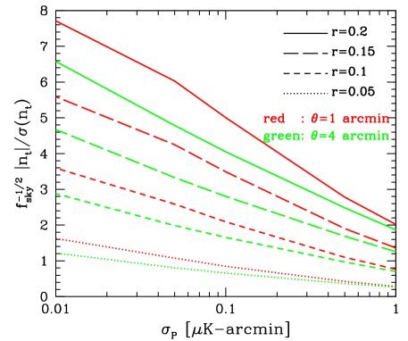
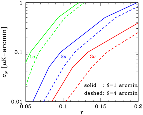
Figure 1: Left: Statistical significance to confirm the consistency relation, $f_{\rm sky}^{-1/2}\,|n_{\rm t}|/\sigma(n_{\mathrm{t}})$, with the fiducial value of the spectral tilt given by $n_{\rm t}=-r/8$. The results for tensor-to-scalar ratios $r=0.2$ (solid), $0.15$ (long dashed), $0.1$ (short dashed), and $0.05$ (dotted) are plotted as a function of the polarization sensitivity $\sigma_{\mathrm{P}}$ in units of $\mu$K-arcmin. The red and green lines, respectively, represent angular resolutions of $\theta=1$ and $4$ arcmin. Right: Required polarization sensitivity to test the consistency relation as a function of the tenor-to-scalar ratio $r$ for a full-sky CMB experiment ($f_{\rm sky}=1$). For the angular resolution $\theta=1$ (solid) and $4$ arcmin (dashed), the required sensitivity $\sigma_{\rm P}$ is shown at the statistical significance of $1\sigma$ (green), $2\sigma$ (blue), and $3\sigma$ (red) levels.

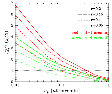
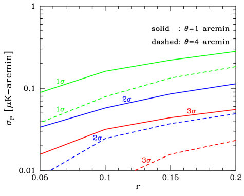
Figure 2: Left: Signal-to-noise ratio of the lensing curl-mode induced by the primordial gravitational waves $f_{\rm sky}^{-1/2}\,\mbox{(S/N)}_{\varpi\varpi}$ plotted against the sensitivity $\sigma_{\mathrm{P}}$. The meaning of the line types is the same as in the left panel of Fig. 1. As a reference, the $1\sigma$ significance is shown in as the black solid line. Right: Required sensitivity to detect the lensing curl-mode at $1\sigma$ (green), $2\sigma$ (blue), and $3\sigma$ (red) levels. For a full-sky CMB experiment ($f_{\rm sky}=1$), the results are plotted as a function of the tenor-to-scalar ratio $r$. The sold and dashed lines represent the results with angular resolutions of $\theta=1$ and $4$ arcmin, respectively.

In order to derive the required noise level of a polarization measurement needed to test the consistency relation $n_{\mathrm{t}}=-r/8$, we proceed to the Fisher matrix analysis. Here we consider the B-mode polarization alone, since this is the best sensitive probe to test the consistency relation among various CMB observables. The Fisher matrix is given by

$$F_{ij}\equiv\sum_{\ell=2}^{\ell_{\rm max}}\frac{2\ell+1}{2}f_{\mathrm{sky}}\dfrac{\partial\ln\widehat{C}^{\rm BB}_{\ell}}{\partial p_{i}}\dfrac{\partial\ln\widehat{C}^{\rm BB}_{\ell}}{\partial p_{j}}\,,$$ (9)

with $\widehat{C}^{\rm BB}_{\ell}$ being the observed power spectrum given by Eq. (4), whose lensing contributions are replaced with Eq. (7). For simplicity, we ignore the galactic foreground contamination in computing the power spectrum. The quantities $p_{i}$ are free parameters to be determined by the observations, and we here consider the tensor-to-scalar ratio and tensor spectral index as free parameters, i.e., $p_{i}=(r,n_{\mathrm{t}})$. Given the Fisher matrix above, the marginalized expected $1\sigma$ error on $p_{i}$ is estimated to be $\sigma(p_{i})=\sqrt{\{F^{-1}\}_{ii}}$. Below, setting the maximum multipole to $\ell_{\rm max}=1000$, we evaluate the Fisher matrix.

It is commonly known that confirmation of the consistency relation generally requires a polarization measurement with a significantly low-noise level. We, thus, consider the Stage-IV class or even higher-sensitivity experiments in which the polarization sensitivity $\sigma_{\rm P}\lesssim 1\,\mu$K-arcmin and angular resolution $\theta\lesssim 1$ arcmin can be achieved. For comparison, we also show the case with $\theta=4$ arcmin which is close to the angular resolution of the POLARBEAR and POLAR Array. With these experimental setups, we apply the delensing technique, and estimate the expected error on the tensor spectral tilt from the delensed B-mode polarization based on Eq. (9). Note that, throughout the analysis, we assume the consistency relation for setting the fiducial value of $n_{\mathrm{t}}$.

The left panel of Fig. 1 shows the statistical significance to confirm the consistency relation, defined by $|n_{\rm t}|/(\sqrt{f_{\rm sky}}\sigma(n_{\rm t}))$ with the fiducial value of the tensor spectral tilt, $n_{\rm t}=-r/8$. For the tensor-to-scalar ratios of $r=0.2$ (solid), $0.15$ (long dashed), $0.1$ (short dashed), and $0.05$ (dotted), statistical significances are estimated and are plotted as a function of the sensitivity $\sigma_{\rm P}$. Note that thanks to the low noise level of a polarization measurement, the tensor-to-scalar ratio is tightly constrained for the range of our interest in $r$, and, thus, the detection of primordial tensor perturbations is highly significant, i.e., $r/(\sqrt{f_{\rm sky}}\sigma(r))\gg 1$.

As it is anticipated, the confirmation of the consistency relation becomes harder as decreasing the fiducial value of $r$. This is true even with a full-sky ($f_{\rm sky}=1$) and high-angular resolution ($\theta=1$ arcmin) experiment. For instance, for $r<0.05$, the sensitivity of $\sigma_{\rm P}\ll 0.1\,\mu$K-arcmin is required to confirm the consistency relation. This is more clearly seen when we plot the required sensitivity $\sigma_{\rm P}$ as a function of the tensor-to-scalar ratio. The right panel of Fig. 1 plots the required sensitivity based on the result in the left panel. Here, assuming full-sky observations ($f_{\rm sky}=1$), the results with statistical significance at the $1\sigma$ (green), $2\sigma$ (blue), and $3\sigma$ (red) levels are particularly shown. For a small tensor-to-scalar ratio $r\lesssim 0.1$, a solid confirmation of the consistency relation at the $\gtrsim 3\sigma$ level is rather challenging even for a high-sensitivity experiment of $\sigma_{\rm P}\gtrsim 0.01\,\mu$K-arcmin.

III.2 Detecting gravitational-wave induced lensing

Having confirmed that testing the consistency relation generally requires a high-sensitivity B-mode measurement, we next consider the feasibility to detect the gravitational-wave induced lensing. We estimate the expected signal-to-noise ratio for the reconstructed curl-mode. The signal-to-noise ratio of the curl mode is defined as

$$\left(\frac{\rm S}{\rm N}\right)_{\varpi\varpi}\equiv\left[\sum_{\ell=2}^{\ell_{\rm max}}\frac{2\ell+1}{2}f_{\mathrm{sky}}\left(\frac{C_{\ell}^{\varpi\varpi}}{\widehat{C}_{\ell}^{\varpi\varpi}}\right)^{2}\right]^{1/2}\,.$$ (10)

Note that the observed power spectrum of the curl mode $\widehat{C}^{\varpi\varpi}_{\ell}$ is expressed as

$$\widehat{C}^{\varpi\varpi}_{\ell}=C_{\ell}^{\varpi\varpi}+N_{\ell}^{\varpi}\,,$$ (11)

with the reconstruction noise $N_{\ell}^{\varpi}$ given by Eq. (8).

The left panel of Fig. 2 shows the expected signal-to-noise ratio for the curl mode as a function of the sensitivity $\sigma_{\rm P}$. On the other hand, right panel of Fig. 1 plots the required sensitivity to detect the curl mode as a function of $r$. Here we set $\ell_{\rm max}=1000$ . Similar to the test of the consistency relation, the detectability of the curl mode increases with the fiducial value of $r$. However, one noticeable point is that the required sensitivity for the detection of the gravitational-wave induced lensing is less severe than that for the test of the consistency relation. Indeed, the gravitational-wave induced lensing for $r\,\raise 2.9pt\hbox{$\scriptstyle>$}\lower 0.5pt\hbox{$\scriptscriptstyle\sim$}\;0.1$ will be detected with $3\sigma$ significance if the sensitivity of $\sigma_{\rm P}=0.03\,\mu$K-arcmin is achieved in future CMB experiments. In particular, even if the consistency relation is still difficult to probe, the curl mode would be detected for $r<0.1$. This implies that the high-sensitivity measurement of the curl mode can be a complementary probe of the primordial gravitational waves, offering an independent confirmation from future CMB experiments.

IV Implication to postrecombination gravitational waves

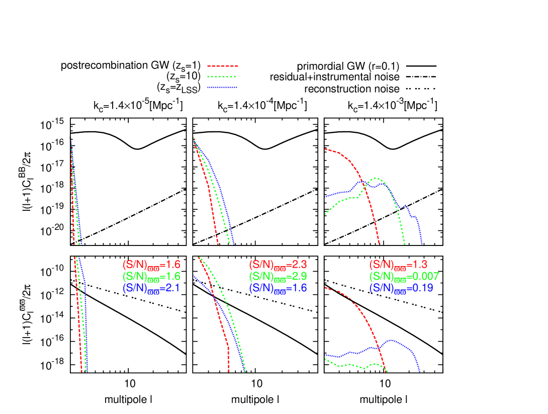
Figure 3: Angular power spectra of the B-mode polarization (top) and lensing curl-mode (bottom) induced by the postrecombination gravitational waves. For specific source redshifts at $z_{\mathrm{s}}=1$ (red), $10$ (green) and $z_{\rm LSS}=1100$ (blue), the expected signals of the B-mode polarization and curl mode are shown. Left, middle, and right panels, respectively, show the results from the postrecombination gravitational waves produced at the frequencies $k_{\mathrm{c}}=1.4\times 10^{-5}$, $1.4\times 10^{-4}$, and $1.4\times 10^{-3}$   Mpc^-1 (see the text for details). The amplitude of the gravitational waves given by $\Delta_{\rm GW}^{2}$ is normalized in each case such that the measured B-mode power spectrum has $(\mbox{S/N})_{\rm BB}=1$. For reference, we also plot in each panel the angular power spectra from the primordial gravitational waves, assuming the tensor-to-scalar ratio, $r=0.1$ (black solid). The noise contributions from the instrument and the lensing reconstruction or delensing are also depicted as dot-dashed lines in each panel.

As another benefit to search for the gravitational-wave induced lensing via a high-sensitivity CMB experiment, we here discuss the gravitational waves generated after the recombination. As we mentioned in Sec. I, there are several mechanisms to produce the late-time gravitational waves: the second-order primordial density perturbations Baumann:2007zm and anisotropic stress of a scalar field in modified gravity theories (see, e.g., Saltas:2014dha ). While the postrecombination gravitational waves lead additional features in both the angular power spectra of the B-mode polarization and curl mode, the curl mode is found to be particularly sensitive to the late-time gravitational waves on large scales.

For illustrative purposes to show how the B-mode polarization and curl mode are sensitive to the postrecombination gravitational waves, we consider gravitational waves emitted instantaneously at a single source plane of $z=z_{\mathrm{s}}$, with a narrow frequency range, $k_{\mathrm{c}}(1-\epsilon)\leq k\leq k_{\mathrm{c}}(1+\epsilon)$. In what follows, we set $\epsilon=0.28$. Adopting the same transfer function as used in the case of the primordial gravitational waves, we compute additional contributions to the angular power spectrum from the postrecombination gravitational waves denoted by $\Delta C^{\rm XX}_{\ell}$, as

$$\Delta C^{\rm XX}_{\ell}= 4\pi\int^{k_{\mathrm{c}}(1+\epsilon)}_{k_{\mathrm{c}}(1-\epsilon)}{\rm d}\ln k\,\Delta_{\rm GW}^{2}$$

$$\times\biggl{[}\int_{0}^{\chi(z_{\mathrm{s}})}{\rm d}\chi\,T(k,\eta_{0}-\chi)S_{{\rm X},\ell}(k,\chi)\biggr{]}^{2}\,.$$ (12)

Here, $T$ is the transfer function and $S_{{\rm X},\ell}$ represents the weight function [e.g., Eq. (3)]. In the above, the quantity $\Delta_{\rm GW}$ represents the amount of the gravitational waves produced at $z_{s}$, and it is treated as a free parameter.

Fig. 3 shows the angular power spectra of the B-mode polarization (top) and curl mode (bottom) from the postrecombination gravitational waves with three different frequencies: $k_{\rm c}=1.4\times 10^{-5}$ (left), $1.4\times 10^{-4}$ (middle), and $1.4\times 10^{-3}$ (right)   Mpc^-1. Here, the amplitude of the gravitational waves $\Delta_{\rm GW}$ is normalized in each case in such a way that the expected signal-to-noise ratio of the B-mode polarization $(\mbox{S/N})_{\rm BB}$ becomes unity .

Overall, the long-wavelength gravitational waves produce a very sharp feature in the angular power spectra. As indicated in Fig. 3, although general trends of the power spectra are rather similar in both the B-mode polarization and lensing curl-mode, resultant signal-to-noise ratios of the curl mode $(\mbox{S/N})_{\varpi\varpi}$ are higher than those of the B-mode polarization especially for smaller $k_{\mathrm{c}}$ and lower $z_{\mathrm{c}}$. This suggests that the curl mode gives a better constraint on the abundance of the postrecombination gravitational waves.

In order to quantify the potential power of the high-sensitivity CMB experiment to constrain the postrecombination gravitational waves, we estimate the expected $1\sigma$ upper bounds on $\Delta_{\mathrm{GW}}^{2}$ based on the following log-likelihood:

$$-2\ln\mathcal{L} =\sum_{\ell=2}^{\ell_{\rm max}}\,(2\ell+1)$$

$$\qquad\times\bigg{[}\frac{\widehat{\mathcal{C}}_{\ell}^{\rm XX}}{\widetilde{\mathcal{C}}_{\ell}^{\rm XX}}+\ln\widetilde{\mathcal{C}}_{\ell}^{\rm XX}-\frac{2\ell-1}{2\ell+1}\ln\widehat{\mathcal{C}}_{\ell}^{\rm XX}\bigg{]}\,.$$ (13)

Here the observed power spectra $\widehat{\mathcal{C}}_{\ell}^{\rm XX}$ are obtained by performing the lensing analysis, and we assume that these have no contribution from the postrecombination sources. On the other hand, $\widetilde{\mathcal{C}}_{\ell}^{\rm XX}$ is a theoretically-estimated power spectrum, which includes the contribution from the postrecombination gravitational waves $\Delta C_{\ell}^{\rm XX}$ on top of the observed power spectrum $\widehat{\mathcal{C}}_{\ell}^{\rm XX}$. In computing the likelihood above, we set the maximum multipole to $\ell_{\rm max}=1000$. The $1\sigma$ constraint on the amplitude $\Delta_{\rm GW}$ is then obtained for the range of frequency centered at $k_{c}$, $k_{\mathrm{c}}(1-\epsilon)\leq k\leq k_{\mathrm{c}}(1+\epsilon)$. For convenience, we translate this constraint into the upper bounds on the spectral energy density at the present time, frequently used in the literature:

$$\Delta\Omega_{\mathrm{GW}}(k)\equiv\frac{1}{\rho_{\mathrm{c}}}\dfrac{{\rm d}\Delta\rho_{\mathrm{GW}}}{{\rm d}\ln k}\biggl{|}_{\eta=\eta_{0}}=\frac{\Delta_{\mathrm{GW}}^{2}}{12H_{0}^{2}}\left(\dfrac{\partial T(k,\eta)}{\partial\eta}\right)^{2}\bigg{|}_{\eta=\eta_{0}}\,,$$ (14)

where $\rho_{\mathrm{c}}$ is the critical density of the Universe, and $H_{0}$ is the Hubble parameter today.

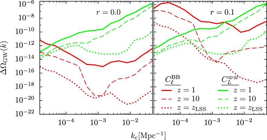
Figure 4: Upper bounds on the spectral energy density of the postrecombination gravitational waves $\Delta\Omega_{\mathrm{GW}}$ as a function of the frequency. The left panel shows the results in the absence of the primordial gravitational waves $(r=0)$, while right panel represents the cases with nonzero primordial gravitational waves of the tensor-to-scalar ratio, $r=0.1$. In each panel, the constraints from the B-mode polarization and lensing curl-mode are depicted as green and red lines, respectively. The solid, dashed, and dotted lines represent the upper bounds on the postrecombination gravitational waves emitted at $z_{\rm s}=1$, $10$, and $z_{\rm LSS}=1100$. We specifically set the experimental parameters to $\sigma_{\rm P}=0.1$ $\mu$K-arcmin and $\theta=1$ arcmin.

In Fig. 4, setting the experimental parameters to $\sigma_{\rm P}=0.1$ $\mu$K-arcmin and $\theta=1$ arcmin specifically, we estimate the expected upper bounds on $\Delta\Omega_{\mathrm{GW}}$ for the postrecombination gravitational waves emitted at $z_{s}=1$ (solid), $10$ (dashed), and $z_{\rm LSS}$ (dotted), and the results are plotted as a function of the frequency . The left panel shows the results in the absence of the primordial gravitational waves. The upper bounds obtained from the curl mode become gradually tight as decreasing the frequency. At $k_{c}\sim 10^{-5}$ Mpc^-1, the constraint eventually becomes comparable to that from the B-mode polarization. On the other hand, the right panel shows the case including the nonzero primordial gravitational waves of $r=0.1$. Note that with the sensitivity of $\sigma_{\rm P}=0.1$ $\mu$K-arcmin, the detection of the primordial gravitational waves via the lensing curl-mode is statistically less significant, i.e., $(S/N)_{\varpi\varpi}<2$ (see Fig. 2). Nevertheless, the upper bounds from the curl mode almost remain the same as in the case of $r=0$, while those from the B-mode polarization substantially become worse. As a result, the curl mode gives a much tighter constraint on the long-wavelength gravitational waves of $k_{c}\,\raise 2.9pt\hbox{$\scriptstyle<$}\lower 0.5pt\hbox{$\scriptscriptstyle\sim$}\;10^{-3}\,$Mpc^-1. Compared to the constraint from the B-mode polarization, this could give a significant improvement by more than $3$ orders of magnitude. The main reason for these results comes from the fact that the contributions of the primordial gravitational waves give rise to a large cosmic variance leading to a significant impact on the large-scale B-mode polarization, while the noise contributions to the curl mode are basically given by the reconstruction noise which hardly changes even in the presence of the primordial gravitational waves. Another notable point in Fig. 4 is that irrespective of the amplitude of the primordial contribution, the constraints on $\Delta\Omega_{\rm GW}$ from the curl mode have a weaker dependence on the source redshift $z_{\rm s}$ than those from the B-mode polarization. Hence, combining the B-mode polarization with the curl mode, we could obtain the stringent constraints on the postrecombination gravitational waves over wide frequency ranges and source redshifts.

V Summary

In this paper, based on the iterative technique for the lensing reconstruction and delensing, we have studied the future detectability of the gravitational-wave induced lensing from a high-sensitivity CMB experiment. The Fisher matrix analysis has revealed that the lensing curl-mode induced by the primordial gravitational waves with $r\lesssim 0.1$ would be detected at more than $3\sigma$ significance where the consistency relation is still hard to confirm. As an implication of searching for the gravitational-wave induced lensing, we have considered the possibility to tightly constrain the postrecombination gravitational waves. We then have found that the lensing curl-mode is particularly sensitive to long-wavelength gravitational waves ($k\,\raise 2.9pt\hbox{$\scriptstyle<$}\lower 0.5pt\hbox{$\scriptscriptstyle\sim$}\;10^{-3}\,$Mpc^-1) produced at $z_{\mathrm{s}}<10$. With a high-sensitivity experiment which will be able to confirm the consistency relation at a few-$\sigma$ level, the lensing curl-mode gives a tighter constraint on their spectral energy density $\Omega_{\mathrm{GW}}$, compared to the one from B-mode polarization by more than $3$ orders of magnitude.

In this paper, we have assumed that the lensing B-mode polarization is generated only from the gradient mode and has no contributions from the curl mode. Ref. Li:2006si showed that the contributions from the curl mode to the lensing B-mode is about $<1\%$ of those from the gradient mode to the lensing B-mode if $r\sim 0.3$. Thus, we would safely ignore the curl-mode contributions to the lensing B-mode as long as we consider the primordial gravitational waves of $r\,\raise 2.9pt\hbox{$\scriptstyle<$}\lower 0.5pt\hbox{$\scriptscriptstyle\sim$}\;0.3$ and the experiment with $\sigma_{\mathrm{P}}\,\raise 2.9pt\hbox{$\scriptstyle>$}\lower 0.5pt\hbox{$\scriptscriptstyle\sim$}\;0.05\mu$K-arcmin. In other words, such contributions have to be seriously taken into account for a future ultra-high-sensitivity experiment. Another concern in the ultra-high-sensitivity experiment would be the rotation of the polarization basis, which can be induced by the primordial gravitational waves Dai:2013nda . The contributions from the higher-order gradient-mode power spectrum $\mathcal{O}[(C_{\ell}^{\phi\phi})^{2}]$ may be also important in estimating the lensing B-mode in high-sensitivity experiments. These issues are left for our future work.

- (1) BICEP2 Collaboration , “Detection of B-Mode Polarization at Degree Angular Scales by BICEP2”, Phys.Rev.Lett. 112 (2014) 241101, [arXiv:1403.3985].
- (2) Planck Collaboration , “Planck intermediate results. XXX. The angular power spectrum of polarized dust emission at intermediate and high Galactic latitudes”, arXiv:1409.5738.
- (3) K. Abazajian et al., “Inflation Physics from the Cosmic Microwave Background and Large Scale Structure”, Astropart. Phys. 63 (2015) 55–65, [arXiv:1309.5381].
- (4) K. Abazajian et al., “Neutrino Physics from the Cosmic Microwave Background and Large Scale Structure”, Astropart. Phys. 63 (2015) 66–80, [arXiv:1309.5383].
- (5) SPTpol Collaboration , D. Hanson et al., “Detection of B-mode Polarization in the Cosmic Microwave Background with Data from the South Pole Telescope”, Phys.Rev.Lett. 111 (2013), no. 14 141301, [arXiv:1307.5830].
- (6) POLARBEAR Collaboration , “Measurement of the Cosmic Microwave Background Polarization Lensing Power Spectrum with the POLARBEAR experiment”, Phys.Rev.Lett. 113 (2014) 021301, [arXiv:1312.6646].
- (7) L. Boyle et al., “On testing and extending the inflationary consistency relation for tensor modes”, arXiv:1408.3129.
- (8) G. Simard, D. Hanson, and G. Holder, “Prospects for Delensing the Cosmic Microwave Background for Studying Inflation”, arXiv:1410.0691.
- (9) C. M. Hirata and U. Seljak, “Reconstruction of lensing from the cosmic microwave background polarization”, Phys. Rev. D 68 (2003) 083002, [astro-ph/0306354].
- (10) A. Cooray, M. Kamionkowski, and R. R. Caldwell, “Cosmic shear of the microwave background: The curl diagnostic”, Phys. Rev. D71 (2005) 123527, [astro-ph/0503002].
- (11) T. Namikawa, D. Yamauchi, and A. Taruya, “Full-sky lensing reconstruction of gradient and curl modes from CMB maps”, JCAP 1201 (2012) 007, [arXiv:1110.1718].
- (12) S. Dodelson, E. Rozo, and A. Stebbins, “Primordial gravity waves and weak lensing”, Phys. Rev. Lett. 91 (2003) 021301, [astro-ph/0301177].
- (13) C. Li and A. Cooray, “Weak Lensing of the Cosmic Microwave Background by Foreground Gravitational Waves”, Phys.Rev. D74 (2006) 023521, [astro-ph/0604179].
- (14) D. Baumann, P. J. Steinhardt, K. Takahashi, and K. Ichiki, “Gravitational Wave Spectrum Induced by Primordial Scalar Perturbations”, Phys. Rev. D76 (2005) 084019, [hep-th/0703290].
- (15) D. Yamauchi, T. Namikawa, and A. Taruya, “Full-sky formulae for weak lensing power spectra from total angular momentum method”, JCAP 1308 (2013) 051, [arXiv:1305.3348].
- (16) I. D. Saltas, I. Sawicki, L. Amendola, and M. Kunz, “Anisotropic stress as signature of non-standard propagation of gravitational waves”, arXiv:1406.7139.
- (17) E. Fenu, D. G. Figueroa, R. Durrer, and J. Garcia-Bellido, “Gravitational waves from self-ordering scalar fields”, JCAP 10 (oct, 2009) 5, [arXiv:0908.0425].
- (18) D. G. Figueroa, M. Hindmarsh, and J. Urrestilla, “Exact Scale-Invariant Background of Gravitational Waves from Cosmic Defects”, Physical Review Letters 110 (mar, 2013) 101302, [arXiv:1212.5458].
- (19) A. Rotti and T. Souradeep, “New Window into Stochastic Gravitational Wave Background”, Phys. Rev. Lett. (2012).
- (20) Planck Collaboration , “Planck 2013 results. XVI. Cosmological parameters”, Astron. Astrophys. 571 (2014) A16, [arXiv:1303.5076].
- (21) A. Lewis, A. Challinor, and A. Lasenby, “Efficient Computation of CMB anisotropies in closed FRW models”, Astrophys. J. 538 (2000) 473–476, [astro-ph/9911177].
- (22) K. M. Smith et al., “Delensing CMB Polarization with External Datasets”, JCAP 1206 (2012) 014, [arXiv:1010.0048].
- (23) W. Wu et al., “A Guide to Designing Future Ground-based Cosmic Microwave Background Experiments”, Astrophys.J. 788 (2014) 138, [arXiv:1402.4108].
- (24) T. Okamoto and W. Hu, “CMB Lensing Reconstruction on the Full Sky”, Phys. Rev. D67 (2003) 083002, [astro-ph/0301031].
- (25) L. Dai, “Rotation of the cosmic microwave background polarization from weak gravitational lensing”, Phys.Rev.Lett. 112 (2014), no. 4 041303, [arXiv:1311.3662].