Absence of collapse in quantum Rabi oscillations

Abstract

We show analytically that the collapse and revival in the population dynamics of the atom-cavity coupled system under the rotating wave approximation (RWA), valid only at very weak coupling, is an artifact as the atom-cavity coupling is increased. Even the first-order correction to the RWA is able to bring about the absence of the collapse in the dynamics of atomic population inversion thanks to intrinsic oscillations resulting from the transitions between two levels with the same atomic quantum number. The removal of the collapse is valid for a wide range of coupling strengths which are accessible to current experimental setups. In addition, based on our analytical results that greatly improve upon the conventional RWA, even the strong-coupling power spectrum can now be explained with the help of the numerically exact energy levels.

I introduction

The collapse and revival in the population dynamics of the atom-cavity coupled system under the rotating wave approximation (RWA) is an important issue in quantum optics Scully . The collapse is attributed to the destructive interference among various transitions between the atomic upper and lower levels, and the revival is due to quantized nature of the photonic number states in the cavity. The collapse and revival phenomenon was first predicted by Eberly et al. eberly ; eberly1 , and was observed experimentally by Rempe et al. rempe .

The RWA is a very good approximation if the atom-cavity interaction energy is much smaller than the characteristic energy of the atom-cavity coupled system, i.e., if the ratio of the coupling constant and the field frequency, $g/\omega$, is much less than unity, a parameter space often refereed to as the weak coupling regime. If the coupling constant is comparable to the field frequency, i.e., $g/\omega\approx 0.1$, also known as the ultra-strong coupling regime, the counter-rotating terms (CRTs) have to be considered. The effect of the CRTs on the dynamics of the atomic population inversion has been studied in the weak coupling regime Muller ; zubairy as well as the deep strong coupling regime with $g/\omega>1$ Casanova . Zhang et al. examined the full range of atom-cavity coupling finding that the collapse and revival gradually disappear and reemerge periodically as the coupling strength increases in the strong coupling regime Zhangyy . Numerically exact calculations reveal that the collapse and revival gradually loses prominence as the coupling is increased, and vanish in the ultra-strong coupling regime. However, due to the lack of an analytical apparatus analogous to RWA, an in-depth understanding remains elusive on the dynamics of atomic population inversion from the weak to the ultra-strong coupling regime ($g/\omega\leq 0.2$).

For superconducting qubits, a one-dimensional transmission-line resonator, or an LC circuit Wallraff ; Chiorescu ; Wang ; Fink ; Deppe can play the role of the cavity, also known as the circuit quantum electrodynamics (QED) systems. Recently, an LC resonator inductively coupled to a superconducting qubit Niemczyk ; exp ; Mooij has been realized experimentally. The qubit-resonator coupling $g/\omega$ has been strengthened to $\thicksim 0.1$, entering the ultra-strong coupling regime, and evidence for the breakdown of the RWA has been provided Niemczyk . Therefore, the CRTs can no longer be ignored. Recently, much attention has been devoted to the qubit-oscillator system and the effect of the CRTs in the ultra-strong coupling regime Werlang ; Hanggi ; Nori ; Hausinger ; chen10b ; Zhang13 .

A two-level atom coupled to a single-mode cavity has long been a subject of extensive study, for which two main schemes are usually employed. One is based on the phontonic Fock states as pioneered by Swain Swain ; Kus ; Durstt ; Tur ; Bishop , and the other, on various unitary transformations or displaced oscillators Feranchuk ; Irish ; chenqh ; liu ; chen10 ; zheng ; QingHu1 ; Braak ; exp ; Beaudoin ; Chen2012a ; zhao94 ; wu2013 , which are equivalent to extended coherent states chen94 or extended squeezed states Nori . Very accurate solutions can be obtained in the latter scheme, but as an infinite number of phontonic Fock states are involved, certain important features may be smeared out.

Recently, He et al. proposed a method of using only the dominant parts in Swain’s wave function Chen2012b in the corrections to the RWA. The effect of the CRTs emerges clearly even in the first-order correction. All eigenvalues and eigenfunctions are derived analytically. The vacuum Rabi splitting has been obtained successfully up to the remarkable coupling strength of $g=0.4$, suggesting that they could be convincingly applied to recent circuit QED systems operating in the ultra-strong coupling regime. In this work, we show that this method can be improved further with easy-to-use eigenvalues and eigenvectors similar to those in the RWA, and the atomic population inversion from an initial field of coherent states can then be studied in great detail.

The paper is organized as follows. In Section II, we show an improved version of the first correction to the RWA, and give all eigensolutions similar as those in RWA. In Section III, the atomic population inversion is calculated analytically. The origin of the absence of the collapse up to the ultra-strong coupling regime is examined in detail. The structure of the exact power spectrum is discussed in terms of the corrections to the RWA and the numerical exact energy levels. A brief summary is given in Section IV.

II Corrected rotating-wave approximations

The Hamiltonian of a two-level atom (a qubit) with transition frequency $\Delta$ interacting with a single-mode quantized cavity of frequency $\omega$ takes the form

$$H=\frac{\Delta}{2}\sigma_{z}+\omega a^{\dagger}a+g\left(a^{\dagger}+a\right)\sigma_{x},$$ (1)

where $g$ is coupling strength, $\sigma_{x}$ and $\sigma_{z}$ are Pauli spin-$1/2$ operators, and $a^{\dagger}$ and $a$ are the creation and annihilation operators for the quantized field. Here we define $\delta=\Delta-\omega$ as the detuning parameter, and focus on the resonance case of $\delta=0$. The frequency of the cavity mode is set to unity as the energy scale, i.e., $\omega=1$.

The RWA neglects the CRTs, $a^{\dagger}\sigma_{+}+a\sigma_{-}$, rendering the Hamiltonian diagonalizable with the eigenfunctions Scully

$$\left|kn\right\rangle^{\mathrm{RWA}}=\frac{1}{\sqrt{2}}\left(\ \begin{array}[]{l}\left(-1\right)^{k}\;\left|n\right\rangle\\ \ \left|n+1\right\rangle\end{array}\right),~{}k=1,2,~{}n=0,1,2,...$$ (2)

and the corresponding eigenvalues

$$E_{kn}^{\mathrm{RWA}}=n+\frac{1}{2}+\left(-1\right)^{k}\sqrt{n+1}g,$$ (3)

where $k=1,2$ is the atomic quantum number, and $n=0,1,2,...$ is the photonic quantum number. Throughout this appear, $n$ and $k$ are regarded as the level indices.

A unified expression in the first-order correction to the RWA was proposed for the eigenvalues and eigenfucntions in a recent work Chen2012b , which recovers the RWA expression in the absence of the correction. In this paper, we employ an improved selection rule for the roots of the derived univariate cubic equation, and obtain a modified general expression with details given below.

The first correction to the RWA wave function is to add a new photonic state $\left|n+2\right\rangle$ to the upper atomic level so that the wave function can be written as

$$\left|kn\right\rangle=\left(\ \begin{array}[]{l}c_{kn}^{(0)}\left|n\right\rangle+c_{kn}^{(2)}\left|n+2\right\rangle\\ \;\;\;\;\;c_{kn}^{(1)}\left|n+1\right\rangle\end{array}\right).$$ (4)

From the RWA results, we note that an odd quantum number $n$ is for even parity, and an even $n$ for odd parity, resulting in a single univariate cubic equation

$$E^{3}-\left(3n+\frac{7}{2}\right)E^{2}+\left[\left(n+\frac{1}{2}\right)\left(3n+\frac{11}{2}\right)-\left(2n+3\right)g^{2}\right]E$$

$$-\left(n+\frac{1}{2}\right)^{2}\left(n+\frac{5}{2}\right)+\left(2n^{2}+6n+\frac{7}{2}\right)g^{2}=0,$$ (5)

which is the same as Eq. (22) in Ref. Chen2012b . In Sec. III (B)1 of Ref. Chen2012b , however, a scenario of an even quantum number $n$ with even parity and an odd $n$ with odd parity was also considered, which does not arise in Hamiltonian (1) where only one univariate cubic equation is needed to account for all physical results. Note that Eq. (5) in principle gives three roots. Comparing with the RWA results, we know that each $n$ corresponds to two eigenvalues, one of which is superfluous and should be omitted. By fitting the numerically exact results, two roots are chosen:

$$E_{kn}=\frac{\left(3n+\frac{7}{2}\right)+\sqrt{\allowbreak\left(6n+9\right)g^{2}+4}\left[\cos\theta+\left(-1\right)^{k}\sqrt{3}\sin\theta\right]}{3},$$ (6)

where

$$\theta=\frac{1}{3}\arccos\left(\frac{-8+9ng^{2}}{\sqrt{\left[4+\left(6n+9\right)g^{2}\right]^{3}}}\right)+\frac{2\pi}{3},$$

and the ratio of coefficients in the eigenfunctions (4) is

$$c_{kn}^{(0)}:c_{kn}^{(1)}:c_{kn}^{(2)}=\left[-\frac{\sqrt{n+1}}{\Omega_{n}(E_{kn})}\right]:1:\left[-\frac{\sqrt{n+2}}{\Omega_{n+2}(E_{kn})}\right],$$ (7)

with

$$\Omega_{n}(E_{kn})=\frac{1}{g}\left[n-E_{kn}+\frac{\Delta}{2}\right].$$

Eqs. (4) and (6) are the counterparts of RWA results, Eqs. (2) and (3).

It is easily seen that the leading wave function correction $\left|\uparrow,n+2\right\rangle$ in the upper atomic level is produced by the CRTs, $a^{\dagger}\sigma_{+}+a\sigma_{-}$. This first correction to RWA, which will be denoted as CRWA, is responsible for numerous physical processes beyond the RWA, and with eigenvalues and eigenvectors explicitly given, corresponding to the RWA results one by one, applications of CRWA can be conveniently made.

To better compare with the RWA, the CRWA eigenvalues can be expanded in terms of the coupling constant $g$ as follows

$$E_{kn}=n+\frac{1}{2}+\left(-1\right)^{k}\sqrt{n+1}g-\frac{n+2}{4}g^{2}-\left(-1\right)^{k}\frac{\left(n+2\right)\left(3n+2\right)}{32\sqrt{n+1}}g^{3}+O(g^{3}),$$ (8)

and the three coefficients in the normalized eigenfunctions read

$$c_{kn}^{(0)}=(-1)^{k}\frac{\sqrt{2}}{2}+\frac{\sqrt{2}(n+2)}{16\sqrt{n+1}}g-(-1)^{k}\frac{\sqrt{2}(n+2)^{2}}{256(n+1)}g^{2}+O(g^{2}),$$

$$c_{kn}^{(1)}=\frac{\sqrt{2}}{2}-(-1)^{k}\frac{\sqrt{2}(n+2)}{16\sqrt{n+1}}g-\frac{\sqrt{2}(n+2)(17n+18)}{256(n+1)}g^{2}+O(g^{2}),$$

$$c_{kn}^{(2)}=-\frac{\sqrt{2n+4}}{4}g-(-1)^{k}\frac{(3n+2)\sqrt{2n+4}}{32\sqrt{n+1}}g^{2}+O(g^{2}).$$ (9)

Comparing Eq. (8) with the RWA counterpart Eq. (3), it is found that the conventional RWA results are recovered if only 1st-order (in $g$) terms are kept in Eq. (8). A similar comparison between Eq. (9) and Eq. (2) reveals that the RWA eigenstates appear explicitly in the expressions of the CRWA counterparts. It makes sense that the coefficients $c_{kn}^{(0)}$and $c_{kn}^{(1)}$ of $\left|\uparrow n\right\rangle$ and$\ \left|\downarrow n+1\right\rangle\;$in the RWA states, respectively, are of order $1$, and coefficients$\ c_{kn}^{(2)}$ for the new state $\left|\uparrow n+2\right\rangle$ are of order $g$. It will be demonstrated that the CRWA expansions are exact up to $g^{2}$ ($g$) in energy (wave function). Here we keep one higher order term in both the eigenvalues and eigenvectors, which can be shown to reproduce Eqs. (6) and (4) with sufficient accuracy, and will therefore be used to calculate all CRWA results in this work. As the CRWA eigenvectors are approximate, they are not all strictly orthogonal. For example, for $k_{1}\neq k_{2},$ $\left\langle k_{1}n\right|\left|k_{2}n\right\rangle\propto g^{4}\neq 0$. It is understood that orthogonality is only observed in the weak coupling limit.

Following the standard procedure, we can also obtain the ground state (GS) and its energy by adding one new bare state to the RWA one $\left|\downarrow 0\right\rangle$ as

$$\left|GS\right\rangle=\left(\ \begin{array}[]{l}\;d_{1}\left|1\right\rangle\\ \;d_{0}\left|0\right\rangle\end{array}\right),$$ (10)

where

$$d_{0} = \allowbreak 1-\frac{1}{8}g^{2}+\frac{11}{128}g^{4},$$

$$d_{1} = -\frac{1}{2}g+\frac{3}{16}g^{3},$$

and

$$E_{GS}=-\frac{1}{2}-\frac{1}{2}g^{2}+\frac{1}{8}g^{4}.$$ (11)

This GS eigenvector is regarded as the CRWA one, because only one new phontonic state is added, analogous to the CRWA excited states.

Similarly, we can also obtain the GS energy and state with higher order corrections

$$E_{GS}^{(2)} = -\frac{1}{2}-\frac{1}{2}g^{2}-\frac{1}{8}g^{4}+O\left(g^{6}\right),$$ (12)

$$\left|GS\right\rangle^{(2)} = \left(\ \begin{array}[]{l}\;\;\;\;d_{1}^{(2)}\left|1\right\rangle\\ d_{0}^{(2)}\left|0\right\rangle+d_{2}^{(2)}\left|2\right\rangle\end{array}\right),$$ (15)

with

$$d_{0}^{(2)} = 1-\frac{1}{8}g^{2}-\frac{13}{128}g^{4}+O\left(g^{6}\right),$$

$$d_{1}^{(2)} = -\allowbreak\frac{1}{2}g-\frac{1}{16}g^{3}+O\left(g^{5}\right),$$

$$d_{2}^{(2)} = \frac{\sqrt{2}}{4}g^{2}-\frac{\sqrt{2}}{32}g^{4}+O\left(g^{6}\right).$$

It is interesting to note that the eigenvalues (eigenvectors) up to $g^{2}$ ($g$) in the CRWA are not modified in the second corrections of the GS state. The GS eigenvectors appear to reveal the general property of the excited states with second order corrections, for which analytical expressions are elusive.

CRWA may not yield more accurate results than many other approaches involving infinitely many photon states. The advantage, instead, lies in the transparency in important mechanisms of interest provided by the compact eigenstates with only three photonic number states. Now with all CRWA eigenvalues and eigenvectors at hand, we can revisit many physical problems that have been studied using the RWA. In this paper, we focus on the quantum dynamical effects, one fundamental issue in quantum optics.

III atomic population inversion from coherent state

III.1 The CRWA Results

We first consider a two-level atom interacting with a coherent field. The initial coherent state in the upper level can be expanded in terms of the photonic number states

$$\left|\alpha\right\rangle=\sum_{n}\beta_{n}\left|\uparrow,n\right\rangle,$$ (16)

where $\beta_{n}=\exp\left(-\left|\alpha\right|^{2}/2\right)\frac{\alpha^{n}}{\sqrt{n!}}$ is a Poisson distribution , $\alpha^{2}=\overline{n}\;$ is the average photon number.

It is well known that the atomic population inversion exhibits collapse followed by periodic revivals in the RWA Scully . It is intriguing to ask what would happen beyond the RWA. Using the CRWA results given in Eqs. (8) and (9), one can easily calculate the dynamics of the atomic population inversion. The results are presented in Fig. 1 for $\alpha^{2}=10$ and two coupling strengths $g=0.02$ and $0.06$. The corresponding RWA results are also shown in Fig. 1 with differences accounted for by the CRTs. To demonstrate the validity of the CRWA, we compare in the inset of Fig. 1 the numerically exact results with the CRWA counterparts in two time periods of large oscillation amplitudes. Surprisingly, our CRWA results are in excellent agreement with the exact ones up to the ultra-strong coupling regime (with $g$ in the order of $0.1$). Actually, the agreement can be kept up to $g=0.2$ (not shown here), a coupling strength almost doubling the current experimentally accessible value.

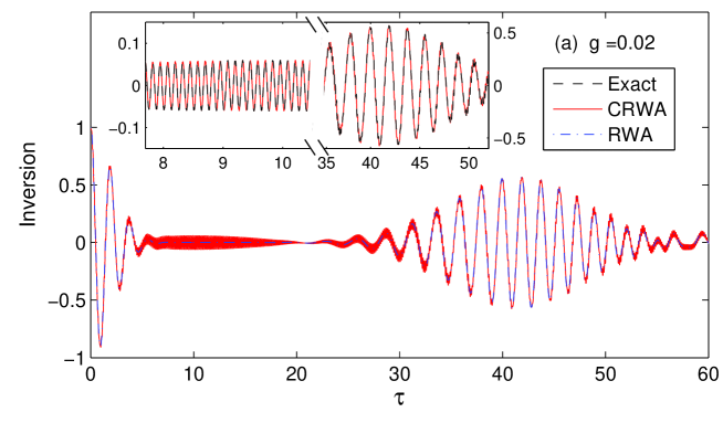
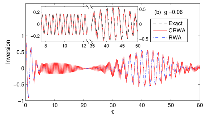
Figure 1: (Color online) The atomic population inversion for an initial coherent state for $g=0.02$ and $0.06$ using the CRWA (solid red), the RWA ( dashed-dotted blue), and numerically exact calculations ( dashed black) with an average photon number $\alpha^{2}=10$. The reduced time $\tau=2gt$.

Interestingly, a new oscillation appears during the collapses with a coupling-independent frequency and an amplitude roughly proportional to the coupling strength. This is to say, the well-known collapse observed in the RWA is absent due to the presence of the CRTs, even at a very weak coupling strength (such as $g=0.02$), where the RWA is usually considered to be valid. While it is difficult for certain accurate approaches based on an infinite series of number states to uncover this mysterious phenomenon, here we will derive the atomic population inversion analytically and discuss the detailed dynamics based on the CRWA with only one new state added to the RWA one.

III.2 Detailed process in terms of CRWA

We can expand the initial coherent state in the upper level in terms of the CRWA eigenstates, and then obtain the atomic population inversion. We list here individual contributions for the benefit of discussion leaving detailed derivations to Appendix A:

$$W(t)=\left(2C-1\right)+2\sum_{k=1,2}S_{k}\cos[(E_{GS}-E_{k1})t]+W^{(\mathrm{Rabi})}(t)+W_{sk}^{(I)}(t)+W_{dk}^{(I)}(t),$$ (17)

where

$$W^{(\mathrm{Rabi})}(t)=2\sum_{n=0}^{\infty}R_{n}\cos\left[(E_{2n}-E_{1n})t\right],$$ (18)

$$W_{sk}^{(I)}(t) = 2\sum_{n=0}^{\infty}\left\{I_{1n}\cos\left[\left(E_{1n}-E_{1n+2}\right)t\right]+I_{2n}\cos\left[\left(E_{2n}-E_{2n+2}\right)\right]t\right\},$$ (19)

$$W_{dk}^{(I)}(t) = 2\sum_{n=0}^{\infty}\left\{I_{12n}\cos\left[(E_{1n}-E_{2n+2})t\right]+I_{21n}\cos\left[(E_{2n}-E_{1n+2})t\right]\right\},$$ (20)

where all coefficients are given in Eqs. (38) in Appendix A. In Eq. (17), the first constant term and the second terms for transitions to the GS state are extremely small for $g\leq 0.2$, and can be omitted. The main contributions to the atomic population inversion are the three kinds of oscillations given by Eqs. (18), (19), and (20). Eq. (18) depicts the modified Rabi oscillations, which are not essentially different from the usual one in the RWA. Eqs. (19) and (20) describe the transitions between the ($k,n$) and ($k,n+2$) levels, and those between the ($k,n$) and ($k^{\prime}\neq k,n+2$) levels, respectively.

To show contributions individually, we calculate Eqs. (18), (19), and (20) independently. Fig. 2 (a) shows the three contributions for $g=0.06$. The black lines depict the atomic population inversion for the transitions between the ($k,n$) and ($k,n+2$) levels, revealing the absence of the usual collapse. For the transitions between the ($k,n$) and ($k^{\prime}\neq k,n+2$) levels, the atomic population inversion, as shown by the red lines, displays the collapse and revivals as in the Rabi oscillations. The modified Rabi oscillations are shown as the blue lines. The main results in Fig. 1(b) can then be completely reproduced by summing up these three contributions.

To better illustrate the point, we collect the amplitude terms up to order $g$ and the energy difference terms up to order $g^{2}$ in Eq. (40), obtaining a concise expression for the atomic population inversion:

$$W(t)=\sum_{n=0}^{\infty}\beta_{n}^{2}\left[\cos\left[(E_{2n}-E_{1n})t\right]-\frac{g\alpha^{2}}{2\sqrt{n+1}}\sum_{k,k^{\prime}=1,2}\left(-1\right)^{k^{\prime}}\cos\left[\left(E_{k,n+2}-E_{k^{\prime},n}\right)t\right]\right],$$ (21)

where

$$E_{2n}-E_{n}=2\sqrt{n+1}g,$$ (22)

$$E_{k,n+2}-E_{k,n}=2-\frac{g^{2}}{2}+\left(-1\right)^{k}g\left(\sqrt{n+3}-\sqrt{n+1}\right),$$ (23)

$$E_{k,n+2}-E_{k^{\prime}\neq k,n}=2-\frac{g^{2}}{2}+\left(-1\right)^{k}g\left(\sqrt{n+3}+\sqrt{n+1}\right).$$ (24)

The first term in Eq. (21) is the conventional Rabi oscillation, which can be approximated by $\cos\left(2gt\sqrt{\alpha^{2}+1}\right)e^{-\frac{1}{2}\left(gt\right)^{2}}$ at short times ($gt<\alpha$). The collapse occurs at $t_{\mathrm{collapse}}\thicksim 1/g$ due to the exponential factor, and the usual Rabi frequency is $2g\sqrt{\alpha^{2}+1}$. The second term in Eq. (21) includes four oscillations. All are from the transitions between $(k,n)$ and $(k,n+2)$ levels, which, despite being ubiquitous in exact dynamics even for weak coupling, are absent in the RWA. In fact, the inter-level oscillations, also known as the intrinsic oscillations, are even captured by semi-classical descriptions of two-level atoms coupled with a classical field.

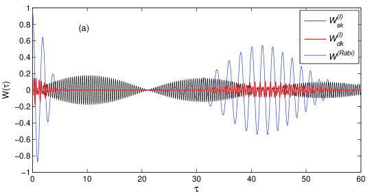
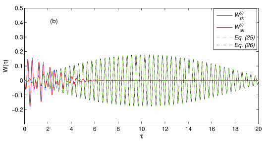
Figure 2: (Color online) (a) Various contributions to the time dependent atomic population inversion: $W^{(I)}_{sk}$ for transitions from the levels in different $n$ with the same $k$ , and $W^{(I)}_{dk}$ with different $k$, modified Rabi oscillations $W^{(\mathrm{Rabi})}(t)$ at $g=0.06$, $\alpha^{2}=10$. (b) Comparisons with the approximate short-time dynamics given in Eqs. (27) and (28). The reduced time $\tau=2gt$.

Now we focus on the energy difference, i.e., the frequency of the oscillations. It is observed that the energy differences with the same $k$ [Eq. (21)] are very small, and those with the different $k$ [Eq. (22)] are large. Regrouping the summation in the second term of Eq. (21) yields

$$W_{sk}^{(I)}(t)=g\alpha^{2}\sin\left[\left(2-\frac{1}{2}g^{2}\right)t\right]\sum_{n=0}^{\infty}\frac{\beta_{n}^{2}}{\sqrt{n+1}}\sin\left[g\left(\sqrt{n+3}-\sqrt{n+1}\right)t\right],$$ (25)

$$W_{dk}^{(I)}(t)=-g\alpha^{2}\sin\left[\left(2-\frac{1}{2}g^{2}\right)t\right]\sum_{n=0}^{\infty}\frac{\beta_{n}^{2}}{\sqrt{n+1}}\sin\left[g\left(\sqrt{n+1}+\sqrt{n+3}\right)t\right].$$ (26)

Note that they share a common fast oscillation with a weakly $g$-dependent frequency of $2-\frac{1}{2}g^{2}$. However, their envelopes are given by different infinite summations.

Considering the weight $\beta_{n}$ in the summation, the dominate term in the envelope of Eq. (25) is from the $n=\alpha^{2}$ term, so the short-time dynamics is roughly described by

$$W_{sk}^{(I)}(t)\thickapprox\frac{g\alpha^{2}}{\sqrt{\alpha^{2}+1}}\sin\left[\left(2-\frac{1}{2}g^{2}\right)t\right]\sin\left[\frac{gt}{\sqrt{\alpha^{2}+1}}\right].$$ (27)

As shown in Fig. 2 (b) by the green line, Eq. (25) describes the short-time dynamics very well. It is well known that the first collapse under the RWA persists up to the revival time $\tau_{\mathrm{revival}}=2\pi\alpha$. For $\alpha^{2}>>1$, the argument in the second sin function in Eq. (27) at the revival time is about $\pi$. So in the RWA collapse regime, this fast oscillation in the CRWA is enveloped sinusoidally with a half period with a maximum amplitude of about $g\alpha$. For the given parameters, the first revival time is $\tau_{\mathrm{revival}}\thickapprox 20$, and the half period for the first envelope should be also approximately $20$, which is just in excellent agreement with Fig. 2 (b). Actually for any average photonic number, there is no finite collapse regime for the fast oscillations in the short-time dynamics. It follows that there is absolutely no collapse in the absence of RWA.

While the other intrinsic oscillations described by Eq. (26) at short times can be approximated by

$$W_{dk}^{(I)}(t)\thickapprox-g\alpha\sin\left[\left(2-\frac{1}{2}g^{2}\right)t\right]\sin(2g\alpha t)\exp\left[-\frac{\left(gt\right)^{2}}{2}\right].$$ (28)

The detailed derivation is presented in Appendix B. It is also demonstrated by the blue line in Fig. 2 (b) that the above approximation can capture the short-time dynamics quite well. Note that the intrinsic oscillations from the transitions between ($k,n$) and ($k^{\prime}\neq k,n+2$) levels also collapse at the same time as the Rabi oscillations thanks to the same decay factor $\exp\left[-\left(gt\right)^{2}/2\right]$ such that they do not contribute to the absence of the collapse at all.

To sum up, the transitions between levels of $n$ and $n+2$ with the same $k$ bring about a fast intrinsic oscillation with amplitude $g\alpha$, which is remarkable so that the collapse actually never occur in the real system. Previous collapse is only an artificial results from the theoretical RWA. As exhibited in Fig. 1 even for $g=0.02$, a visible intrinsic oscillation appears in the usual RWA collapse regime. As the coupling strength in the current circuit QED systems has reached $g=0.1$, the absence of collapse can be checked experimentally.

We believe that a first order perturbation technique in the path integral framework zubairy would give similar results to order $g$ at weak coupling. Their findings were attributed to the CRTs as a whole, and mechanisms relevant to the transitions are elusive due to the fact that detailed information on the eigenstates is not available in the path integral approach which integrates out all bosonic degrees of freedom. In addition, compared with the exact solution, our CRWA results may not be better than the second-order perturbative one, but an infinite number of phontonic Fock states are involved in the second-order perturbation theory, depriving its analytical clarity.

III.3 Power spectrum

To probe further various oscillations in the atomic population inversion, we calculate the power spectrum $F(\omega)$ defined as follows

$$F(\omega)=\left|\int_{0}^{\infty}W(t)\exp\left(-i\omega\ t\right)dt\right|^{2}.$$ (29)

The power spectrum will be calculated exactly and analyzed using our CRWA results, in which various transitions can be identified separately.

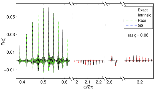
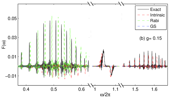
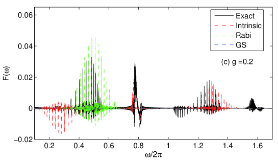
Figure 3: (Color online) The power spectrum for $g=0.06,0.15$, and $0.2$ with CRWA and numerical exact study at average photon number $\alpha^{2}=10$. The frequency unit is $2g$.

In Fig. 3, the numerically exact power spectrum for various coupling strengths are given by solid black lines for the case of $\alpha^{2}=10$. We also list the power spectrum individually from different time-dependent components such as the Rabi oscillations (green lines) and intrinsic oscillations (red lines) in Eq. (21). It is very interesting that all the power spectra obtained analytically in the CRWA can find their counterparts in the exact spectrum, and the agreement is good up to $g=0.2$.

Next, let us analyze the structure of the spectrum in the CRWA in the time scale of $\tau=2gt$. The Rabi frequency is centered around $\omega_{R}/2\pi=$ $\sqrt{\alpha^{2}+1}/2\pi=0.53$, independent of $g$, and therefore appear in the same position. The Rabi oscillations in the CRWA are qualitatively the same as those in RWA. A slight deviation from the exact ones with an increase in the coupling strength is due to a small deviation of the CRWA energy levels from the exact solutions.

The intrinsic oscillations from the CRTs are not captured by the RWA. The two frequencies from intrinsic transitions within same $k$, $\omega_{k}^{s}$, are given by Eq. (23), where two dominate frequencies come from $n\thickapprox\alpha^{2}$ levels

$$\omega_{k}^{s}=\left[2-\frac{g^{2}}{2}+\left(-1\right)^{k}g\left(\sqrt{\alpha^{2}+3}-\sqrt{\alpha^{2}+1}\right)\right]/2g.$$ (30)

Note that the third term in Eq. (23) is very small compared to the central frequency $\omega_{c}=\left(1-g^{2}/4\right)/g$, and is weakly dependent on $n$. So they appear sharply in the two side of the central frequency $\omega_{c}$. The other two frequencies from transitions between different $k$’s, $\omega_{k}^{d}$, are given by Eq. (24). Two dominate frequencies from $n\thickapprox\alpha^{2}\$ levels are given by

$$\omega_{k}^{d}=\left[2-\frac{g^{2}}{2}+\left(-1\right)^{k}g\left(\sqrt{\alpha^{2}+3}+\sqrt{\alpha^{2}+1}\right)\right]/2g.$$ (31)

From Eq. (24), we note however that the third term is comparable with the central frequency $\omega_{c}$, and is strongly dependent on $n$. Therefore, broad peaks appear on the two sides of the two dominate ones, $\omega_{k}^{d}$, in the power spectrum, as demonstrated in the exact solutions. The peak positions from the four dominate frequencies calculated from Eqs. (30) and (31) also coincide with the exact ones.

For $g=0.06$, the spectra calculated from the CRWA are in excellent agreement with the numerically exact ones. As the coupling strength is increased to $g=0.15$ and $0.2$, the aforementioned four CRWA frequencies from Eqs. (30) and (31) and the Rabi peak, which are in the low frequency regime and dominate the atomic population inversion, remain in agreement with the exact ones. Thus, we have demonstrated that the main features in the power spectrum of the numerically exact solutions can be explained analytically by the CRWA. We note that a weak, broad spectral feature, which becomes pronounced only at strong coupling, also appears at the high frequencies, and cannot be reproduced in the CRWA.

After analyzing the structure of the wave function, it becomes clear that the new intrinsic oscillation from the further corrections to the RWA should take the form

$$\sim g^{2}\alpha^{2}\exp\left(-\alpha^{2}\right)\sum_{k,k^{\prime}=1,2}\sum_{n=0}^{\infty}\frac{1}{\sqrt{n+3}}\frac{\alpha^{2n}}{n!}\cos\left(E_{k,n+4}t-E_{k^{\prime},n}t\right),$$ (32)

$$\sim g^{3}\alpha^{2}\exp\left(-\alpha^{2}\right)\sum_{k,k^{\prime}=1,2}\sum_{n=0}^{\infty}\frac{1}{\sqrt{n+5}}\frac{\alpha^{2n}}{n!}\cos\left(E_{k,n+6}t-E_{k^{\prime},n}t\right).$$ (33)

They are added to the total intrinsic oscillation gradually with the increasing coupling. The amplitude in the $m$-th order corrections is of order $g^{m}$, and therefore they only play a minor effect at weak coupling. With the increasing coupling, they gradually gain importance. We can in principle predict the relevant frequencies of these higher-order intrinsic oscillations that emerge with the increasing coupling.

From Eq. (27), it becomes immediately possible to obtain the next $4$ new intrinsic typical frequencies in the second-order corrections to the RWA

$$\Omega_{k}^{s} = \left[4-g^{2}+\left(-1\right)^{k}g\left(\sqrt{\alpha^{2}+5}-\sqrt{\alpha^{2}+1}\right)\right]/2g,$$ (34)

$$\Omega_{k}^{d} = \left[4-g^{2}+\left(-1\right)^{k}g\left(\sqrt{\alpha^{2}+5}+\sqrt{\alpha^{2}+1}\right)\right]/2g,$$ (35)

Note that the CRWA energy levels will still be used due to the lack of analytical solutions in the second order corrections to the RWA. The peak positions calculated from the equations above using the CRWA energy are in agreement with the numerically exact ones for $g=0.15$ and $g=0.2$, as shown in Figs. 3 (b) and (c). The small deviation from the exact spectra are attributed to the approximate CRWA energies. Were numerically exact energy levels used, the agreement should be much improved.

IV summary

In summary, using the CRWA, we have studied analytically the atomic population inversion from an initial coherent field. The often-seen collapse in the RWA is found to be wiped out by intrinsic oscillations attributed to the transitions between ($k,n$) and ($k^{\prime}=k,n+2$) levels. As the intrinsic oscillations are ubiquitous in atom-cavity coupled systems as long as the CRTs are taken into account, it is concluded that the collapse is just an artifact of the RWA. In addition, we have analyzed the power spectrum of the atomic population inversion, finding the analytical CRWA spectrum in excellent agreement with that from the exact solutions in the ultra-strong coupling regime. As the coupling is further increased, the main characteristic frequencies can be well accounted for by the CRWA. Second-order corrections to the RWA are shown to be able to explain additional features in the power spectrum calculated from the exact solutions. Finally, our prediction on the absence of the collapse can be checked experimentally in the ultra-strong coupling regime.

V ACKNOWLEDGEMENTS

We acknowledge useful discussion with Shi-Yao Zhu and Yu-Yu Zhang. This work is supported by National Basic Research Program of China (China), 2011CBA00103 , National Natural Science Foundation of China (China), 11174254, 11474256, , and the Singapore National Research Foundation through the Competitive Research Programme (CRP), NRF-CRP5-2009-04.

^∗ Corresponding author. Email:qhchen@zju.edu.cn

Appendix A Derivation of the atomic population inversion

The initial coherent state in the upper atomic level can be expanded as

$$|\psi(0)\rangle=\exp(-\alpha^{2}/2)|\uparrow\rangle\sum_{n=0}\frac{\alpha^{n}}{\sqrt{n!}}|n\rangle=|\uparrow\rangle\sum_{n=0}\beta_{n}|n\rangle,$$ (36)

In terms of CRWA eigenstates, the time dependent state in $|\uparrow,n\rangle$ can be expressed in detail as follows. For $n=0$

$$\sum_{k=1,2}\left[\beta_{0}(c_{k0}^{(0)})^{2}+\beta_{2}c_{k0}^{(2)}c_{k0}^{(0)}\right]e^{-iE_{k0}t},$$

for $n=1$

$$\sum_{k=1,2}\left[\beta_{1}(c_{k1}^{(0)})^{2}+\beta_{3}c_{k1}^{(2)}c_{k1}^{(0)}\right]e^{-iE_{k1}t}+\beta_{1}(d_{1})^{2}e^{-iE_{GS}t},$$

and generally $n\geq 2$

$$\sum_{k=1,2}\left[\beta_{n-2}c_{kn-2}^{(0)}c_{kn-2}^{(2)}+\beta_{n}(c_{kn-2}^{(2)})^{2}\right]e^{-iE_{kn-2}t}+\left[\beta_{n}(c_{kn}^{(0)})^{2}+\beta_{n+2}c_{kn}^{(0)}c_{kn}^{(2)}\right]e^{-iE_{kn}t}.$$

Then the upper part of time dependent wave function can be written as

$$|\psi(t)\rangle=\sum_{n=0}\sum_{k=1,2}\left[\beta_{n}c_{kn}^{(0)}c_{kn}^{(2)}+\beta_{n+2}(c_{kn}^{(2)})^{2}\right]e^{-iE_{kn}t}|n+2\rangle$$

$$+\sum_{n=0}\sum_{k=1,2}\left[\beta_{n}(c_{kn}^{(0)})^{2}+\beta_{n+2}c_{kn}^{(0)}c_{kn}^{(2)}\right]e^{-iE_{kn}t}|n\rangle+\beta_{1}(d_{1})^{2}e^{-iE_{GS}t}|1\rangle$$

$$=\sum_{n=0}\sum_{k=1,2}\left[h_{kn}e^{-iE_{kn}t}|n+2\rangle+f_{kn}e^{-iE_{kn}t}|n\rangle\right]+\beta_{1}(d_{1})^{2}e^{-iE_{GS}t}|1\rangle,$$ (37)

where

$$f_{kn}=\beta_{n}(c_{kn}^{(0)})^{2}+\beta_{n+2}c_{kn}^{(0)}c_{kn}^{(2)}=\beta_{n}\left[\frac{1}{2}+(-1)^{k}\frac{1}{8}\frac{(n-2\alpha^{2}+2)}{\sqrt{n+1}}g-\frac{1}{8}\alpha^{2}g^{2}\right],$$

$$h_{kn}=\beta_{n}c_{kn}^{(0)}c_{kn}^{(2)}+\beta_{n+2}(c_{kn}^{(2)})^{2}=\beta_{n}\left[-(-1)^{k}\frac{1}{4}\sqrt{n+2}g+\frac{1}{8}\sqrt{\frac{n+2}{n+1}}(\alpha^{2}-n-1)g^{2}\right].$$

The probability to find the atom in the upper level is then obtained

$$P(t) =C+\sum_{k=1,2}S_{k}\cos[(E_{GS}-E_{k1})t]+\sum_{n=0}\{R_{n}\cos(E_{2n}-E_{1n})t+I_{1n}\cos(E_{1n}-E_{1n+2})t$$

$$+I_{2n}\cos(E_{2n}-E_{2n+2})t+I_{12n}\cos(E_{1n}-E_{2n+2})t+I_{21n}\cos(E_{2n}-E_{1n+2})t\},$$

where

$$R_{n}=2(f_{1n}f_{2n}+h_{1n}h_{2n})=\frac{1}{2}\beta_{n}^{2}\left[1-(\frac{\alpha^{2}}{2}+\frac{1}{16}\frac{(n-2\alpha^{2}+2)^{2}}{n+1}+\frac{1}{4}n+\frac{1}{2})g^{2}\right],$$

$$I_{1n}=2h_{1n}f_{1n+2}=\frac{1}{2}\beta_{n}^{2}\left\{\left[-\frac{1}{8}\frac{(n+4-2\alpha^{2})}{\sqrt{n+1}\sqrt{n+3}}+\frac{1}{4}\frac{(\alpha^{2}-n-1)}{n+1}\right]\alpha^{2}g^{2}+\frac{1}{2}\frac{\alpha^{2}g}{\sqrt{n+1}}\right\},$$

$$I_{2n}=2h_{2n}f_{2n+2}=\frac{1}{2}\beta_{n}^{2}\left\{\left[-\frac{1}{8}\frac{(n+4-2\alpha^{2})}{\sqrt{n+1}\sqrt{n+3}}+\frac{1}{4}\frac{(\alpha^{2}-n-1)}{n+1}\right]\alpha^{2}g^{2}-\frac{1}{2}\frac{\alpha^{2}g}{\sqrt{n+1}}\right\},$$

$$I_{12n} =2h_{1n}f_{2n+2}=\frac{1}{2}\beta_{n}^{2}\left\{\left[\frac{1}{8}\frac{(n+4-2\alpha^{2})}{\sqrt{n+1}\sqrt{n+3}}+\frac{1}{4}\frac{(\alpha^{2}-n-1)}{n+1}\right]\alpha^{2}g^{2}+\frac{1}{2}\frac{\alpha^{2}g}{\sqrt{n+1}}\right\},$$

$$I_{21n} =2h_{2n}f_{1n+2}=\frac{1}{2}\beta_{n}^{2}\left\{\left[\frac{1}{8}\frac{(n+4-2\alpha^{2})}{\sqrt{n+1}\sqrt{n+3}}+\frac{1}{4}\frac{(\alpha^{2}-n-1)}{n+1}\right]\alpha^{2}g^{2}-\frac{1}{2}\frac{\alpha^{2}g}{\sqrt{n+1}}\right\},$$

$$C =\sum_{k=1,2}\sum_{n=0}|f_{kn}|^{2}+|h_{kn}|^{2}=\frac{1}{2}+e^{-\alpha^{2}}g^{2}\sum_{n=0}\frac{\alpha^{2n}}{n!}\left[-\frac{1}{4}\alpha^{2}+\frac{1}{32}\frac{(n-2\alpha^{2}+2)^{2}}{n+1}+\frac{n}{8}+\frac{1}{4}\right],$$

$$S_{k} =2f_{1k}d_{1}^{2}\beta_{1}=\frac{1}{4}e^{-\alpha^{2}}\alpha^{2}g^{2}.$$ (38)

The atomic population inversion is therefore easily given by

$$W^{CRWA}(t)=2P(t)-1,$$ (39)

collecting all contribution up to the $g^{2}$  we have

$$W^{CRWA}(t)=\left(2C-1\right)+W_{GS}(t)+W^{(\mathrm{Rabi})}(t)+W^{(I)}(t),$$ (40)

where

$$2C-1=g^{2}\sum_{n=0}\beta_{n}^{2}\left[\frac{1}{2}+\frac{n}{4}-\frac{\alpha^{2}}{2}+\frac{\left(n-2\alpha^{2}+2\right)^{2}}{16\left(n+1\right)}\right],$$ (41)

$$W_{GS}=\alpha^{2}g^{2}e^{-\alpha^{2}}\cos[(2-\frac{g^{2}}{4})t]\cos[(1-\frac{15g^{2}}{64})\sqrt{2}gt],$$ (42)

$$W^{(\mathrm{Rabi})}(t)=\sum_{n=0}\beta_{n}^{2}\left[1-\left(\left(\frac{1}{2}+\frac{n}{4}+\frac{\alpha^{2}}{2}+\frac{\left(n-2\alpha^{2}+2\right)^{2}}{16\left(n+1\right)}\right)g^{2}\right)\right]\cos(E_{2n}-E_{1n})t,$$ (43)

$$W^{(I)}(t) = -\frac{1}{2}g\alpha^{2}\sum_{k,k^{\prime}=1,2}\sum_{n=0}^{\infty}\frac{\beta_{n}^{2}}{\sqrt{n+1}}\left(-1\right)^{k^{\prime}}\cos\left(E_{k,n+2}t-E_{k^{\prime},n}t\right)$$ (46)

$$+\alpha^{2}g^{2}\sum_{n=0}\beta_{n}^{2}\cos\left[\left(2-\frac{1}{2}g^{2}\right)t\right]\left\{\begin{array}[]{c}\frac{(\alpha^{2}-n-1)}{n+1}\cos\left(g\sqrt{n+1}t\right)\cos\left(g\sqrt{n+3}t\right)\\ -\frac{1}{2}\frac{(n+4-2\alpha^{2})}{\sqrt{n+1}\sqrt{n+3}}\sin\left(g\sqrt{n+1}t\right)\sin\left(g\sqrt{n+3}t\right)\end{array}\right\}.$$

Appendix B Approximate short-time dynamics using the saddle-point method

By using the saddle-point method, the asymptotic expansion of integrals of the following form is given by

$$F(\overline{n})=\int_{0}^{\infty}f(n)e^{\overline{n}S(n)}dn=\sqrt{-\frac{2\pi}{\overline{n}S^{\prime\prime}(n_{0})}}\exp\left[\overline{n}S(n_{0})\right]\left[f(n_{0})+O(\overline{n}^{-1})\right],$$ (47)

where $\overline{n}$ is very large, the zeros of $S^{\prime}(n)$ are called the saddle points of $S(n)$.

The envelope of Eq. (25) can be transformed to the following integral [c.f. Ref. (eberly1 )]

$$F (t)= \sum_{n=0}^{\infty}\frac{\beta_{n}^{2}}{\sqrt{n+1}}\sin\left[g\left(\sqrt{n+1}+\sqrt{n+3}\right)t\right],$$

$$= \int_{0}^{\infty}dn\frac{\exp\left[-\overline{n}+n-n\ln\left(\frac{n}{\overline{n}}\right)\right]}{\sqrt{2\pi n}}\frac{1}{\sqrt{n+1}}\sin\left[g\left(\sqrt{n+1}+\sqrt{n+3}\right)t\right],$$

where the Stirling’s approximation was used. By $\cos\left(x\right)+i\sin\left(x\right)=e^{ix}$ , we have

$$F(t) = {Im}\left\{\int_{0}^{\infty}dn\frac{\exp\left[-\overline{n}+n-n\ln\left(\frac{n}{\overline{n}}\right)+i\left(\sqrt{n+1}+\sqrt{n+3}\right)gt\right]}{\sqrt{2\pi n}}\frac{1}{\sqrt{n+1}}\right\},$$

$$= \exp\left(-\overline{n}\right){Im}\left(\int_{0}^{\infty}dn\frac{\exp\left(\overline{n}S(n)\right)}{\sqrt{2\pi n\left(n+1\right)}}\right),$$

where

$$\ S(n)=\frac{n}{\overline{n}}-\frac{n}{\overline{n}}\ln\left(\frac{n}{\overline{n}}\right)+i\frac{\sqrt{n+1}+\sqrt{n+3}}{\overline{n}}gt.$$

The zero of $S^{\prime}(n)\;$give the saddle point $n_{0}$

$$\ln\left(\frac{n_{0}}{\overline{n}}\right)=i\left(\frac{1}{\sqrt{n_{0}+1}}+\frac{1}{\sqrt{n_{0}+3}}\right)\frac{gt}{2}.$$

Considering short-time $gt/\sqrt{\bar{n}}\ll 1,$ so $\frac{n_{0}}{\overline{n}}\rightarrow 1,\;$we have

$$n_{0}\thickapprox\bar{n}(1+\frac{igt}{\sqrt{\bar{n}}}).$$ (48)

By using Eq. (47) , we have

$$F(t)=\exp\left(-\overline{n}\right){Im}\left(\sqrt{-\frac{2\pi}{\overline{n}S^{\prime\prime}(n_{0})}}\exp\left[\overline{n}S(n_{0})\right]\frac{1}{\sqrt{2\pi n_{0}(n_{0}+1)}}\right).$$

Inserting Eq. (48) , we finally obtain

$$F(t)\thickapprox\sqrt{\frac{1}{\bar{n}}}\sin(2g\sqrt{\bar{n}}t)\exp\left[-\frac{\left(gt\right)^{2}}{2}\right].$$ (49)

References

- (1) M. O. Scully and M. S. Zubairy, Quantum Optics (Cambridge University Press, Cambridge, 1997); M. Orszag, Quantum Optics Including Noise Reduction,Trapped Ions, Quantum Trajectories, and Decoherence (Science Publishing Group, New York, 2007).).
- (2) J. H. Eberly, N. B. Narozny, and J. J. Sanchez-Mondragon, Phys. Rev. Lett. 44, 1323(1980).
- (3) N. B. Narozny, J. J. Sanchez-Mondragon, and J. H. Eberly, Phys. Rev. A. 23, 236(1981).
- (4) G. Rempe et al., Phys. Rev. Lett. 58, 353(1987).
- (5) L. Müller, J. Stolze, H. Leschke, and Peter Nagel, Phys. Rev. A 44, 1022(1991); G. A. Finney and J. Gea-Banacloche, Phys. Rev. A 50, 2040 (1994); O. Gat, M. Lein and S. Teufel, J. Phys. A: Math. Theor. 46, 315301 (2013).
- (6) K. Zaheer, and M. S. Zubairy, Phys. Rev. A 37, 1628(1988). The results shown in figures 1 and 2 are reasonable, but Eq. (19) would not yield these figures, probably due to some typos.
- (7) J. Casanova et al., Phys. Rev. Lett. 105, 263603 (2010).
- (8) Y. Y. Zhang, Q. H. Chen, and S. Y. Zhu, Chin. Phys. Lett. 30, 114203 (2013), see also arXiv:1106.2191 (2011).
- (9) A. Wallraff et al., Nature (London) 431, 162 (2004).
- (10) I. Chiorescu et al., Nature 431, 159 (2004). J. Johansson et al., Phys. Rev. Lett. 96, 127006 (2006).
- (11) H. Wang et al., Phys. Rev. Lett. 101, 240401 (2008); M. Hofheinz et al., Nature 459, 546 (2009).
- (12) J. Fink et al., Nature 454, 315 (2008).
- (13) F. Deppe et al., Nature Physics 4, 686 (2008).
- (14) T. Niemczyk et al., Nature Physics 6, 772 (2010).
- (15) P. Forn-Díaz et al., Phys. Rev. Lett. 105, 237001 (2010).
- (16) A. Fedorov et al., Phys. Rev. Lett. 105,060503 (2010).
- (17) T. Werlanget al., Phys. Rev. A 78, 053805 (2008).
- (18) D. Zueco et al., Phys. Rev. A 80, 033846 (2009).
- (19) S. Ashhab and F. Nori, Phys. Rev. A 81, 042311 (2010).
- (20) J. Hausinger and M. Grifoni, Phys. Rev. A 82, 062320(2010).
- (21) Q. H. Chen, L. Li, T. Liu, and K. L. Wang, Chin. Phys. Lett. 29, 014208 (2012); see also arXiv:1007.1747 (2010).
- (22) Y. Y. Zhang, Q. H. Chen, and Y. Zhao, Phys. Rev. A. 87, 033827 (2013).
- (23) S. Swain, J. Phys. A 6, 1919 (1973).
- (24) M. Kus, J. Math. Phys. 26, 2792 (1985); M. Kus and M. Lewenstein, J. Phys. A: Math. Gen. 19, 305 (1986).
- (25) C Durstt, E Sigmundt, P ReinekerS and A Scheuing, J. Phys. C: Solid State Phys. 19, 2701 (1986).
- (26) E. A. Tur, Optics and Spectroscopy COPY 89, 574 (2000).
- (27) R. F. Bishop et al., Phys. Rev. A 54, R4657 (1996); R. F. Bishop and C. Emary, J. Phys. A: Math. Gen. 34, 5635 (2001).
- (28) I. D. Feranchuk, L. I. Komarov and A. P. Ulyanenkov, J. Phys. A: Math. Gen. 29, 4035 (1996).
- (29) E. K. Irish, Phys. Rev. Lett. 99, 173601 (2007).
- (30) Q. H. Chen, Y. Y. Zhang, T. Liu, and K. L. Wang, Phys. Rev. A 78, 051801(R) (2008).
- (31) T. Liu, K. L. Wang, and M. Feng, EPL 86, 54003 (2009).
- (32) Q. H. Chen, Y. Yang, T. Liu, and K. L. Wang, Phys. Rev. A 82, 052306 (2010).
- (33) C. J. Gan, and H. Zheng, Eur. Phys. J. D 59,473 (2010).
- (34) Q. H. Chen, T. Liu, Y. Y. Zhang, and K. L. Wang, Europhys. Lett. 96, 14003 (2011).
- (35) D. Braak, Phys. Rev. Lett. 107, 100401 (2011).
- (36) F. Beaudoin, J. M. Gambetta, and A. Blais, Phys. Rev. A 84, 043832 (2011)
- (37) Q. H Chen, C. Wang, S. He, T. Liu, and K. L. Wang, Phys. Rev. A 86, 023822(2012).
- (38) Y. Zhao, D. Brown, K. Lindenberg, J. Chem. Phys. 100, 2335 (1994).
- (39) N. Wu and Y. Zhao, J. Chem. Phys. 139, 054118 (2013).
- (40) Q. H. Chen et al., Phys. Rev. B 53, 11296(1996); Y. Y. Zhang, Q. H. Chen, and K. L. Wang, Phys. Rev. B 81, 121105 (R)(2010).
- (41) S. He, C. Wang, Q. H Chen, X. Z. Ren, T. Liu, and K. L. Wang, Phys. Rev. A 86, 033837(2012). The results in Fig. 2 for the vacuum Rabi splitting remain unchanged, as we involve only the first three eigenstates, which are not modified in the current CRWA scheme.