Metrics for Probabilistic Geometries

Abstract

We investigate the geometrical structure of probabilistic generative dimensionality reduction models using the tools of Riemannian geometry. We explicitly define a distribution over the natural metric given by the models. We provide the necessary algorithms to compute expected metric tensors where the distribution over mappings is given by a Gaussian process. We treat the corresponding latent variable model as a Riemannian manifold and we use the expectation of the metric under the Gaussian process prior to define interpolating paths and measure distance between latent points. We show how distances that respect the expected metric lead to more appropriate generation of new data.

1 MOTIVATION

One way of representing a high dimensional data set is to relate it to a lower dimensional set of latent variables through a set of (potentially nonlinear) functions. If the $i$th data point and the $j$th feature is represented by $y_{i,j}$, it might be related to a $q$ dimensional vector of latent variables $\mathbf{x}_{i,:}$ as

$$y_{i,j}=f_{j}(\mathbf{x}_{i,:})+\bm{\epsilon}_{i},$$

where $f_{j}(\cdot)$ is a nonlinear function mapping to the $j$th feature of the data set and $\bm{\epsilon}_{i}$ is a noise corruption of the underlying function. A manifold derived from a finite data set can never be precisely determined across the entire input range of $\mathbf{x}$. We consider posterior distributions defined over $f_{j}(\cdot)$ and we focus on the uncertainty defined over the local metric of the manifold itself. This allows us to define distances that are based on metrics that take account of the uncertainty with which the manifold is defined. We use these metrics to define distances between points in the latent space that respect these metrics.

When the mappings $f_{j}(\cdot)$ are nonlinear, the latent variable model (LVM) can potentially capture non-linearities on the data and thereby provide an even lower dimensional representation as well as a more useful view of the data. While this line of thinking is popular, it is not without its practical issues. As an illustrative example, Fig. 1 shows the latent representation of a set of artificially rotated images obtained through a Gaussian process latent variable model (GP-LVM). It is clear from the display that the latent representation captures the underlying periodic structure of the process which generated the data (a rotation). If we want to analyse the data in the latent space, e.g. by interpolating latent points, our current tools are insufficient. As can be seen, fitting a straight line in the latent space between the two-points leads to a solution that does not interpolate well in the data space: the interpolant goes through regions where the data does not reside, regions where the actual functions, $f_{j}(\cdot)$, cannot be well determined.

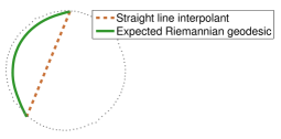
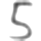
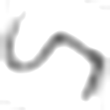
Figure 1: The latent space from a GP-LVM that was trained over a dataset of artificially rotated digits. Black dots represent the latent points. The dashed brown line show the commonly used straight-line interpolant, and the green curve is the suggested expected Riemannian geodesic. This figure is best viewed in colour.

This observation raises several related questions about the choice of interpolant: 1) what is the natural choice of interpolant in the latent space? And, 2) if the natural interpolant is not a straight line, are Euclidean distances still meaningful? We answer these questions for the GP-LVM, though our approach is applicable to other generative models as well. We consider here a metric which reflects the intrinsic properties of the original data and recovers some information loss due to the nonlinear mapping performed by the model. We find that for smooth LVMs the metric from the observation space can be brought back to the latent space in the form of a random Riemannian metric. We then provide algorithms for computing distances and shortest paths (geodesics) under the expected Riemannian metric. With this the natural interpolant becomes a curve, which follows the trend of the data.

Overview

In Section 2 we introduce the concepts of Riemannian geometry, the tool on which we rely on later on in the paper. Section 3 provides an overview of the state of the art in probabilistic dimensionality reduction, introducing the class of models to which the proposed methodology can be extended. In Section 4 we use the probabilistic nature of the generative LVMs to explicitly provide distributions over the metric tensor; first, we provide the general expressions, then we specialise these to the GP-LVM as an example. Finally, we show how to compute shortest paths (geodesics) over the latent space. Experimental results are provided in Section 5, and the paper is concluded with a discussion in Section 6.

2 CONCEPTS OF RIEMANNIAN GEOMETRY

We study latent variable models (LVMs) as embeddings of uncertain surfaces (or manifolds) into the observation space. From a machine learning point of view, we can interpret this embedded manifold as the underlying support of the data distribution. To this end, we review the basic ideas of differential geometry, which study surfaces through local linear models.

Gauss’ study (1827) of curved surfaces is among the first examples of (deterministic) LVMs. He noted that a $q$-dimensional surface embedded in a $p$-dimensional Euclidean space is well-described through a mapping $f:\mathbb{R}^{q}\rightarrow\mathbb{R}^{p}$. The $q$-dimensional representation of the surface is known as the chart (in machine learning terminology, this corresponds to the latent space). In general, the mapping $f$ between the chart and the embedding space is not isometric, e.g. the Euclidean length of a straight line $l$ in the chart does not match the length of the embedded curve $f(l)$ as measured in the embedding space. Intuitively, the chart provides a distorted view of the surface (see Fig. 2 for an illustration). To rectify this view, Gauss noted that the length of a curve is

$$\mathrm{Length}\left(f(l)\right) =\int_{0}^{1}\left\|\frac{\partial f(l(t))}{\partial t}\right\|dt =\int_{0}^{1}\left\|\mathbf{J}\frac{\partial l(t)}{\partial t}\right\|dt,$$ (1)

where $\mathbf{J}$ denotes the Jacobian of $f$, i.e.

$$\left[\mathbf{J}\right]_{i,j}=\frac{\partial f_{i}}{\partial l_{j}}.$$ (2)

Measurements on the surface can, thus, be computed in the chart locally, and integrated to provide global measures. This gives rise to the definition of a local inner product, known as a Riemannian metric.

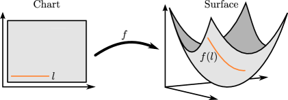
Figure 2: An illustration of the standard surface model; $f$ maps the chart into the embedding space.

Definition (Riemannian Metric).

A Riemannian metric $\mathbf{G}$ on a manifold $\mathcal{M}$ is a symmetric and positive definite matrix which defines a smoothly varying inner product

$$\langle\mathbf{a},\mathbf{b}\rangle_{x} =\mathbf{a}^{\top}\mathbf{J}^{\top}\mathbf{J}\mathbf{b}=\mathbf{a}^{\top}\mathbf{G}(x)\mathbf{b}$$ (3)

in the tangent space $T_{x}\mathcal{M}$, for each point $x\in\mathcal{M}$ and $\mathbf{a},\mathbf{b}\in T_{x}\mathcal{M}$. The matrix $\mathbf{G}$ is called the metric tensor.

Remark

The Riemannian metric need not be restricted to $\mathbf{G}=\mathbf{J}^{\top}\mathbf{J}$ and can be any smoothly changing symmetric positive definite matrix (do Carmo, 1992). We restrict ourselves to the more simple definition as it suffices for our purposes, but note that the more general approach has been used in machine learning, e.g. in metric learning (Hauberg et al., 2012) and information geometry (Amari and Nagaoka, 2000).

From this definition, Eq. 1 reduces to

$$\mathrm{Length}\left(\gamma\right) =\int_{0}^{1}\sqrt{\langle\gamma^{\prime}(t),\gamma^{\prime}(t)\rangle_{\gamma(t)}}dt$$ (4)

for a general curve $\gamma:[0,1]\rightarrow\mathbb{R}^{p}$.

Definition (Geodesic curve).

Given two points $\mathbf{x}_{1},\mathbf{x}_{2}\in\mathcal{M}$, a geodesic is a length-minimising curve connecting the points

$$\gamma_{g}=\arg\min_{\gamma}\mathrm{Length}(\gamma),\quad\gamma(0)=\mathbf{x}_{1},\gamma(1)=\mathbf{x}_{2}.$$ (5)

It can be shown (do Carmo, 1992) that geodesics satisfy the following second order ordinary differential equation

$$\gamma^{\prime\prime} =-\frac{1}{2}\mathbf{G}^{-1}\left[\frac{\partial\operatorname{vec}\mathbf{G}}{\partial\gamma}\right]^{\top}(\gamma^{\prime}\otimes\gamma^{\prime}),$$ (6)

where $\operatorname{vec}\mathbf{G}$ stacks the columns of $\mathbf{G}$ and $\otimes$ denotes the Kronecker product. The Picard-Lindelöf theorem (Tenenbaum and Pollard, 1963) then implies that geodesics exist and are locally unique given a starting point and an initial velocity.

3 PROBABILISTIC DIMENSIONALITY REDUCTION

Nonlinear dimensionality reduction methods (Lee and Verleysen, 2007) provide a flexible data representation which can provide a more faithful model of the observed multivariate datasets than the linear ones. One approach is to perform probabilistic nonlinear dimensionality reduction defining a model that introduces a set of unobserved (or latent) variables $\mathbf{{X}}$ that can be related to the observed ones $\mathbf{Y}$ in order to define a joint distribution over both. These models are known as latent variable models (LVMs). The latent space is dominated by a prior distribution $p(\mathbf{{X}})$ which induces a distribution over $\mathbf{Y}$ under the assumption of a probabilistic mapping

$$y_{i,j}=f_{j}(\mathbf{x}_{i})+\epsilon_{i},$$ (7)

where $\mathbf{x}_{i}$ is the latent point associated with the $i^{th}$ observation $\mathbf{y}_{i}$, $j$ is the index of the features of $\mathbf{Y}$, and $\epsilon_{i}$ is a noise term, accounts for both noise in the data as well as for inaccuracies in the model. The noise is typically chosen as Gaussian distributed $\epsilon\sim\mathcal{N}(0,\beta^{-1})$, where $\beta$ is the precision.

One of the advantages of this approach is that it accommodates dimensionality reduction in an intuitive manner, if we assume that the dimensionality of the latent space is significantly lower than that of the observation space. In this case, the reduced dimensionality provides us with both implicit regularisation and a low-dimensional representation of the data, which can be used for visualisation (and, therefore, for data exploration (Vellido et al., 2011)) if the dimension is low enough.

If the mapping $f=W$ is taken to be linear:

$$y_{i,j}=\mathbf{w}_{j}^{\top}\mathbf{x}_{i}+\epsilon_{i},$$ (8)

and the prior $p(\mathbf{{X}})$ to be Gaussian, this model is known as probabilistic principal component analysis (Tipping and Bishop, 1999). The conditional probability of the data given the latent space can be written as

$$p(\mathbf{y}_{i}\mid\mathbf{x}_{i},\mathbf{W},\beta)=\mathcal{N}(\mathbf{y}_{i}\mid\mathbf{W}\mathbf{x}_{i},\beta^{-1}\mathbf{I}).$$ (9)

With a further assumption of independence across data points, the marginal likelihood of the data is

$$p(\mathbf{Y})=\int\prod_{i=1}^{N}p(\mathbf{y}_{i}\mid\mathbf{x}_{i},\mathbf{W},\beta)p(\mathbf{x}_{i})d\mathbf{{X}}.$$ (10)

In general, this approach can be applied to both linear and nonlinear dimensionality reduction models, leading to the definition of, for instance, Factor Analysis (Bartholomew, 1987), Generative Topographic Mapping (GTM) (Bishop et al., 1998), or Gaussian Process-LVM (GP-LVM) (Lawrence, 2005) to name a few.

One example that generalises from the linear case to the nonlinear one is the GTM, in which the noise model is taken to be a linear combinations of a set of $M$ basis functions

$$y_{i,j}=\sum_{m=i}^{M}\mathbf{w}_{j}^{\top}\phi_{m}(\mathbf{x}_{i})+\epsilon_{i}.$$ (11)

This model can be seen as a mixture of distributions (usually Gaussian radial basis distributions) whose centres are constrained to lay on an intrinsically low-dimensional space. These centres can be interpreted as data prototypes or cluster centroids that can be further agglomerated in a full blown clustering procedure. In this manner, GTM mixes the functionalities of Self-Organising Maps and mixture models by providing both data visualisation over the latent space and data clustering (Olier and Vellido, 2008). If the prior over the latent space is chosen to be Gaussian, this model leads, in a similar way of probabilistic PCA, to a Gaussian conditional distribution of the data

$$p(\mathbf{y}_{i}\mid\mathbf{x}_{i},\mathbf{W},\beta)=\mathcal{N}\left(\mathbf{y}_{i}\left|\sum_{m=i}^{M}\right.\mathbf{w}_{j}^{\top}\phi_{m}(\mathbf{x}_{i}),\beta^{-1}\mathbf{I}\right).$$ (12)

In the classic approach the latent variables are marginalised and the parameters are optimised by maximising the model likelihood. An alternative (and equivalent) approach proposes to marginalise the parameters and optimise the latent variables, leading to Gaussian Process Latent Variables Model (GP-LVM).

In terms of applications, Grochow et al. (2004) animate human poses using style-based inverse kinematics based on a GP-LVM model. The animation is performed under a prior towards small Euclidean motions in the latent space, i.e. under the same assumptions as those leading to a straight-line interpolant. As the Euclidean metric does not match that of the observation space, this prior is difficult to interpret. In a related application, Urtasun et al. (2005) track the pose of a person in a video sequence with a similar prior and, hence, similar considerations hold. Recently, Gonczarek and Tomczak (2014) track human poses in images under a Brownian motion prior in the latent space. Again, this relies on a meaningful metric in the latent space. In all of the above application, it is beneficial if the metric in the latent space is related to that of the observation metric.

4 METRICS FOR PROBABILISTIC LVMs

The common approach to estimate local metrics relies on assumptions over the neighbourhoods defined in the observed space (see e.g. (Hastie and Tibshirani, 1996; Ramanan and Baker, 2011)). This might be less efficient in presence of high dimensional noise, because the induced distances may not be reliable. One way to deal with this problem is to define a noise model (7) and to assume a global belief over the geometry of the data. This way, the resulting models have the advantage of providing an intrinsic local metric which is able to deal with noise.

In this paper we only consider smooth generative models for manifold learning. This contrasts with prior approaches such as (Bregler and Omohundro, 1994; Tenenbaum, 1997; Tenenbaum et al., 2000) that use metrics which vary discretely across the space (see also (Lawrence, 2012) for relations to Gaussian models).

We define here the local metric tensor for generative LVMs. We then illustrate the specific case of GP-LVM, providing an algorithm to compute shortest path.

4.1 THE DISTRIBUTION OF THE NATURAL METRIC

When the mapping $f$ in Eq. 7 is differentiable, it can be interpreted as the mapping between the chart (or latent space) and the embedding space (c.f. Section 2). Then it is possible to explicitly compute the natural Riemannian metric of the given model.

Let $\mathbf{J}$ be the Jacobian (as in Eq. 2), then the tensor

$$\mathbf{G}=\mathbf{J}^{\top}\mathbf{J}$$

defines a local inner product structure over the latent space according to Eq. 3.

In the case of LVMs where the conditional probability over the Jacobian follow a Gaussian distribution, this naturally induces a distribution over the local metric tensor $\mathbf{G}$. Assuming independent rows of $\mathbf{J}$

$$p(\mathbf{J}\mid\mathbf{X},\beta)=\prod_{j=1}^{p}\mathcal{N}(\mathbf{J}_{j,:}\mid\bm{\mu}_{J_{j,:}},\bm{\Sigma}_{J}),$$ (13)

the resulting random variable follow a non-central Wishart distribution (Anderson, 1946):

$$\mathbf{G}=\mathcal{W}_{q}(p,\bm{\Sigma}_{J},\mathbb{E}[\mathbf{J}^{\top}]\mathbb{E}\left[\mathbf{J}\right]),$$ (14)

where $p$ represents the number of degrees of freedom; the quantity $\bm{\Sigma}_{J}^{-1}\mathbb{E}[\mathbf{J}^{\top}]\mathbb{E}\left[\mathbf{J}\right]$ is know as the non-centrality matrix and it is equal to zero in the central Wishart distribution. The Wishart distribution is a multivariate generalisation of the Gamma distribution.

4.2 GP-LVM LOCAL METRIC

A Gaussian Process (GP) is used to describe distributions over functions and it is defined as a collection of random variables, any finite number of which have a joint Gaussian distribution (Rasmussen and Williams, 2006). Given a vector $\mathbf{x}\in\mathbb{R}^{q}$, a GP determined by its mean function and its covariance function is denoted $f(\mathbf{x})\sim\mathcal{GP}(m(\mathbf{x}),k(\mathbf{x},\mathbf{x}^{\prime}))$. From this, it is possible to generate a random vector $\mathbf{f}$ which is Gaussian distributed with covariance matrix given by $(\mathbf{K})_{i,j}=k(\mathbf{x}_{i},\mathbf{x}_{j})$.

Gaussian Processes have been used in probabilistic nonlinear dimensionality reduction to define a prior distribution over the mapping $f$ (in Eq. 7), leading to the formulation of GP-LVM. This way, the likelihood of the data $\mathbf{Y}$ given $\mathbf{{X}}$ is computed by marginalising the mapping and optimising the latent variables:

$$p(\mathbf{{Y}}\!\!\mid\!\mathbf{{X}},\!\beta)\!=\!\!\prod_{j=1}^{p}\!\mathcal{N}(\mathbf{y}_{:,j}\!\mid\!\bm{0},\mathbf{K}\!+\!\beta^{-1}\mathbf{I})\!=\!\!\prod_{j=1}^{p}\!\mathcal{N}(\mathbf{y}_{:,j}\!\!\mid\!\bm{0},\tilde{\mathbf{K}}).$$ (15)

To follow the notation introduced in Section 3, the noise model is defined by

$$y_{i,j}=\tilde{\mathbf{K}}_{(\mathbf{x}_{i},\mathbf{X})}\tilde{\mathbf{K}}\mathbf{Y}_{:,j}+\epsilon_{i},$$ (16)

Due to the linear nature of the differential operator, the derivative of a Gaussian process is again a Gaussian process ((Rasmussen and Williams, 2006) §9.4), as long as the covariance function is differentiable. This property allows inference and predictions about derivatives of a Gaussian Process, therefore the Jacobian $\mathbf{J}$ of the GP-LVM mapping can be computed over continuum for every latent point $\mathbf{x}_{*}$ and we denote with $\frac{\partial\mathbf{y}_{*}}{\partial x^{(i)}}$ the partial derivative of $\mathbf{y}(x_{*})$ with respect to the $i^{th}$ component in the latent space. We call $\mathbf{J}^{\top}_{*}\!=\frac{\partial\mathbf{y}_{*}}{\partial\mathbf{x}}=\!\left[\frac{\partial\mathbf{y}_{*}}{\partial x^{(1)}};\cdots;\frac{\partial\mathbf{y}_{*}}{\partial x^{(q)}}\right]$, where $\frac{\partial\mathbf{y}_{*}}{\partial\mathbf{x}}$ is a $q\times p$ matrix whose columns are multivariate normal distributions. We now consider the jointly Gaussian random variables

$$\left[\begin{array}[]{c}\mathbf{{Y}}\\ \frac{\partial\mathbf{y}_{*}}{\partial\mathbf{x}}\end{array}\right]\sim\mathcal{N}\left(\bf{0},\left[\begin{array}[]{c c}\tilde{\mathbf{K}}_{\bf{x},\bf{x}}&\partial\tilde{\mathbf{K}}_{\bf{x},\bf{*}}\\ \partial\tilde{\mathbf{K}}_{\bf{x},\bf{*}}^{\top}&\partial^{2}\tilde{\mathbf{K}}_{\bf{*},\bf{*}}\end{array}\right]\right),$$ (17)

where $\partial\tilde{\mathbf{K}}_{\bf{*},\bf{x}},\partial^{2}\tilde{\mathbf{K}}_{\bf{*},\bf{*}}$ are a matrices given by

$$(\partial\tilde{\mathbf{K}}_{\bf{x},\bf{*}})_{n,l}=\frac{\partial k(\mathbf{x}_{n},\mathbf{x}_{*})}{\partial x_{*}^{(l)}}, \begin{array}[]{l}n=1,\cdots,N\\ l=1,\cdots,q\end{array}$$ (20)

$$(\partial^{2}\tilde{\mathbf{K}}_{\bf{*},\bf{*}})_{i,l}=\frac{\partial^{2}k(\mathbf{x}_{*},\mathbf{x}_{*})}{\partial x_{*}^{(i)}\partial x_{*}^{(l)}}. \begin{array}[]{l}i=1,\cdots,q\\ l=1,\cdots,q\end{array}$$ (23)

The GP-LVM model provides an explicit mapping from the latent space to the observed space. This mapping defines the support of the observed data $\mathbf{Y}$ as a $q$ dimensional manifold embedded into $\mathbb{R}^{p}$. If the covariance function of the model is continuous and differentiable, the Jacobian of the GP-LVM mapping is well-defined and the natural metric follows Eq. 14.

It follows from Eq. 17 and the properties of the GPs that the distribution of the Jacobian of the GP-LVM mapping is the product of $p$ independent Gaussian distributions (one for each dimension of the dataset) with mean $\bm{\mu}_{J(j,:)}$ and covariance $\bm{\Sigma}_{J}$. For a every latent point $\mathbf{x}_{*}$ the Jacobian takes the following form:

$$p(\mathbf{J}_{*}\mid\mathbf{Y},\mathbf{X},\mathbf{x}_{*})=\prod_{j=1}^{p}\mathcal{N}(\mathbf{J}_{j,:}\mid\bm{\mu}_{J_{j,:}},\bm{\Sigma}_{J})=$$ (24)

$$\prod_{j=1}^{p}\!\mathcal{N}(\mathbf{J}_{j,:}\!\mid\!\partial\tilde{\mathbf{K}}_{\bf{x},\bf{*}}^{\top}\tilde{\mathbf{K}}_{\bf{x},\bf{x}}^{-1}\mathbf{Y}_{:,j}\!,\partial^{2}\tilde{\mathbf{K}}_{\bf{*},\bf{*}}\!\!-\!\partial\tilde{\mathbf{K}}_{\bf{x},\bf{*}}^{\top}\tilde{\mathbf{K}}_{\bf{x},\bf{x}}^{-1}\partial\tilde{\mathbf{K}}_{\bf{x},\bf{*}}\!),$$

which (c.f. Eq. 14) gives a distribution over the metric tensor $\mathbf{G}$

$$\mathbf{G}=\mathcal{W}_{q}(p,\bm{\Sigma}_{J},\mathbb{E}[\mathbf{J}^{\top}]\mathbb{E}[\mathbf{J}]).$$ (25)

From this distribution, the expected metric tensor can be computed as

$$\mathbb{E}[\mathbf{J}^{\top}\mathbf{J}]=\mathbb{E}[\mathbf{J}^{\top}]\mathbb{E}[\mathbf{J}]+p\;\bm{\Sigma}_{J}.$$ (26)

Note that the expectation of the metric tensor includes a covariance term. This implies that the metric tensor expands as the uncertainty over the mapping increases. Hence, curve lengths also increases when going through uncertain regions, and as a consequence geodesics will tend to avoid these regions.

The metric tensor defines the local geometric properties of the GP-LVM model and it can be used as a tool to data exploration. One way to visualise the tensor metric is through the differential volume of the high dimensional parallelepiped spanned by GP-LVM; this, for a latent dimension $q=2$ is known as magnification factor and it has been introduced by (Bishop et al., 1997) for generative topographic mapping (and self organising maps). Its explicit formulation for GP-LVM is given by

$$\mathrm{MF}=\sqrt{\operatorname{det}\left(\mathbb{E}[\mathbf{J}^{\top}\mathbf{J}]\right)}.$$ (27)

An example of the magnification factor is shown in Fig. 3.

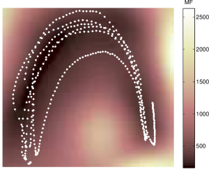
Figure 3: GP-LVM latent space for the motion capture data (see section 5 for details). White dots denote latent points $\mathbf{x}_{n}$ and the background colour is proportional to the magnification factor (27).

4.3 COMPUTING GEODESICS

Given a latent space endowed with an expected Riemannian metric, we now consider how to compute geodesics (shortest paths) between given points. Once a geodesic is computed its length can be evaluated through numerical integration of Eq. 4.

The obvious solution to the shortest path problem is to discretise the latent space and compute shortest paths on the resulting graph using e.g. Dijkstra’s algorithm (Cormen et al., 1990). The computational complexity of this approach, however, grows exponentially with the dimensionality of the latent space and the approach quickly becomes infeasible. Further, this approach will also introduce discretisation errors due to the finite size of the graph.

Instead we solve the geodesic differential equation (6) numerically. This scales more gracefully as it only involves a discretisation of the geodesic curve which is always one-dimensional independently of the dimension of the latent space. The 2nd order ODE in (6) can be rewritten in a standard way as a system of 1st order ODE’s, which we can solve using a four-stage implicit Runge-Kutta method(Kierzenka and Shampine, 2001). This gives a smooth solution which is fifth order accurate. Alternatively, such equations can be solved by repeated Gaussian process regression (Hennig and Hauberg, 2014).

To evaluate Eq. 6 we need the derivative of the expected metric:

$$\frac{\partial\operatorname{vec}\mathbb{E}[\mathbf{G}(\mathbf{x})]}{\partial\mathbf{x}}=\frac{\partial\operatorname{vec}(\mathbb{E}[\mathbf{J}^{\top}]\mathbb{E}[\mathbf{J}]+p\cdot\text{cov}(\mathbf{J},\mathbf{J}))}{\partial\mathbf{x}}.$$ (28)

For the GP-LVM this reduces to computing the derivatives of the covariance function $k$. Given two vectors $\mathbf{x}_{1},\mathbf{x}_{2}\in\mathbb{R}^{q}$, a widely used covariance function is the squared exponential (or RBF) kernel

$$k(\mathbf{x}_{1},\mathbf{x}_{2})=\alpha\,\exp\left(-\frac{\omega}{2}\parallel\mathbf{x}_{1}-\mathbf{x}_{2}\parallel_{2}^{2}\right).$$ (29)

We choose here the RBF as an illustrative example, but our approach apply to any other kernel that leads to a differential mapping. This function is differentiable in $\mathbf{x}$ and will be used here (and in Section 5) to provide a specific algorithm. We explicitly compute Eq. 20 and 23 for the squared exponential kernel to have an explicit form of Eq. 24:

$$\left(\partial\tilde{\mathbf{K}}_{\mathbf{x}_{*},\mathbf{x}}\right)_{1,j}\>\>=\>-\omega(x_{*}^{(j)}-x^{(j)})\,k(\mathbf{x}_{*},\mathbf{x})$$ (30)

$$\left(\partial^{2}\tilde{\mathbf{K}}_{\mathbf{x}_{1},\mathbf{x}_{2}}\right)_{i,l}=$$ (31)

$$=\left\{\begin{array}[]{ll}\omega(x_{1}^{(i)}-x_{2}^{(i)})(x_{1}^{(l)}-x_{2}^{(l)})\,k(\mathbf{x}_{1},\mathbf{x}_{2}),&i\neq l\\ \omega(\omega(x_{1}^{(i)}-x_{2}^{(i)})^{2}-1)\,k(\mathbf{x}_{1},\mathbf{x}_{2}),&i=l\end{array}\right.$$ (34)

Due to symmetry, the upper triangular of the Hessian matrix is sufficient to the computation. Note that, for our choice of kernel, the Hessian is diagonal and constant for $\mathbf{x}_{1}=\mathbf{x}_{2}$, which is the case of $\tilde{\partial^{2}\mathbf{K}_{\bf{*},\bf{*}}}$, so there is no need to compute its derivative (which appears in the expression of $\partial\operatorname{vec}\mathbf{G}$).

5 EXPERIMENTS AND RESULTS

Section 1 shows a first motivating example: a single image of a hand-written digit is rotated from 0 to 360 degrees to produce 200 rotated images. We then estimate a GP-LVM model with a $q=2$ dimensional latent space; the latent space is shown in Fig. 1. We interpolate two points using either a straight line or a geodesic, and reconstruct images along these paths. The results in Fig. 4 show the poor reconstruction of the straight-line interpolator. The core problem with this interpolator is that it goes through regions with little data support, meaning the resulting reconstruction will be similar to the average of the entire data set.

In the next two sections we consider experiments on real data, but our results are similar to the synthetic digit experiment. First, we consider images of rotating objects (Section 5.1), and then motion capture data (Section 5.2).

Figure 4: Rotated digit. Inference after sampling over the latent space following the Geodesic distance (top row) and the Euclidean distance (bottom row); see also Fig. 1. Images are inverted and bicubically upscaled for improved viewing.

5.1 IMAGES OF ROTATING OBJECTS

We consider images from the COIL data set (Nene et al., 1996), which consists of images from a fixed camera depicting 100 different objects on a motorised turntable against a black background. Each image is acquired after a 5 degree rotation of the turntable, giving a total of 72 images per object. Here we consider the images of object $74$ (a rubber duck), but similar results are attained for other objects.

We estimate a $q=2$ dimensional latent space using GP-LVM, and interpolate two latent points using either a straight line or a geodesic. Reconstructed images along the interpolated paths are shown in Fig. 5. It is clear that the geodesic gives a better interpolation as it avoids regions with high uncertainty.

To measure the quality of the different interpolators we reconstruct 50 images equidistantly along each interpolating path and measure the distance to the nearest neighbour in the training data. This is shown in Fig. 6, which, for reference, also shows the average reconstruction error of the latent representations of the training data,

$$\textrm{Avg. training error}=\frac{1}{N}\sum_{n=1}^{N}\|\mathbb{E}\left[f(\mathbf{x}_{n})\right]-\mathbf{y}_{n}\|.$$ (35)

It is clear that the straight line interpolator performs poorly away from the end-points, while the geodesic provides errors which are comparable to the average error of the latent representation of the training data.

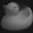
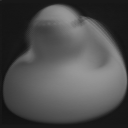
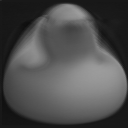
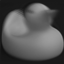
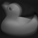
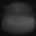
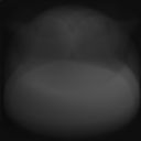
Figure 5: COIL image reconstruction. Inference after sampling over the latent space following the geodesic (top row) and the Euclidean straight line (bottom row).

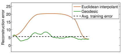
Figure 6: COIL reconstruction error. Inference after sampling over the latent space following the geodesic (green) and the Euclidean straight line (brown). For reference, the average reconstruction error of the latent observations is shown as well (dashed). This figure is best viewed in colour.

5.2 HUMAN MOTION CAPTURE

We next consider human motion capture data from the CMU Motion Capture Database. Specifically, we study motion 16 from subject 22, which is a repetitive jumping jack motion. Each time instance of this data set consists of a human pose as acquired by a marker-based motion capture system; see Fig. 11 for example data. We represent each pose by the three-dimensional joint positions, i.e. as a vector $\mathbf{y}_{n,:}\in\mathbb{R}^{3P}$, where $P$ denotes number of joint positions.

We estimate a GP-LVM using dynamics (Damianou et al., 2011) as is common for this type of data (Wang et al., 2008). The resulting latent space is shown in Fig. 7, and the metric tensor is shown in Fig. 3. As can be seen, the latent points $\mathbf{x}_{n,:}$ follow a periodic pattern as expected for this motion, and the metric tensor is generally smaller in regions of high data density.

We pick two latent extremal points of the motion ($\mathbf{x}_{1}$ and $\mathbf{x}_{T}$) and interpolate them using the Euclidean straight line and the expected Riemannian geodesic. Fig. 7 shows the interpolants: again, the geodesic follow the trend of the data while the straight line goes through regions with high model uncertainty. Reconstructed poses along the interpolants are shown in Fig. 11 and 11. A comparison with the intermediate poses ($\mathbf{x}_{2}\ldots\mathbf{x}_{T-1}$) in the training sequence (see Fig. 11) reveals that the geodesic interpolant is a more truthful reconstruction compared to that of the straight line.

To measure the quality of the reconstruction we note that the length of the subject’s limbs should stay constant throughout the sequence. Our representation does, however, not enforce this constraint. Fig. 8 shows the length of the subjects forearm for the two reconstructions along with the correct length. The straight line interpolant drastically changes the limb lengths, while the geodesic matches the ground truth well. Similar observations have been made for other limbs.

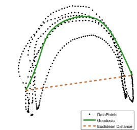
Figure 7: Latent space for the jumping jacks motion capture data, trained with GP-LVM. Black dots denote latent points $\mathbf{x}_{n}$. The green curve denotes the geodesic interpolant, while the dashed brown curve is the straight-line interpolant.

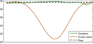
Figure 8: Length, in centimetres, of the subjects forearm during latent space interpolation. The green curve is defined according to the geodesic interpolant, and the brown dashed curve according to the straight-line interpolant. For reference, the black dashed line shows the true length.

Figure 9: Example poses from the motion capture data. These poses are temporarly between the end-points of the interpolating curves, i.e. they are comparable to the interpolated reconstructions.

Figure 10: Interpolated poses according to the straight-line interpolant. In particular, note the bending of the knees and the retraction of the arms, which do not occur in the training data.

Figure 11: Interpolated poses according to the geodesic. These are visually similar to the poses in Fig. 11.

6 DISCUSSION AND FUTURE WORK

When the mapping between a latent space and the observation space is not isometric (the common case for nonlinear mappings), a Euclidean distance measure in the latent space does not match that of the original observation space. In fact, the distance measures in the latent and observation spaces can be arbitrarily different. This makes it difficult to perform any meaningful statistical operation directly in the latent space as the used metric is difficult to interpret.

We solve this issue by carrying the metric from the observation space into the latent space in the form of a random Riemannian metric. This gives a distribution over a smoothly changing local metric at each point in the latent space. We then provide an expression for the expected local metric and show how shortest paths (geodesics) can be computed numerically under the resulting metric. These geodesics provide natural generalisations of straight-lines and are, thus, suitable for interpolation under the new metric.

For the GP-LVM model the expected metric depends on the uncertainty of the model, such that distances become longer in regions of high uncertainty. This effectively forces geodesic curves to avoid uncertain regions in the latent space, which is the desired behaviour for most applications. It is worth noting that a similar analysis for the GTM does not provide a metric with this capacity as the uncertainty is constant in this model.

The idea of considering the expected metric is practical as it turns the latent space into a Riemannian manifold. This opens up to many applications as statistical operations are reasonably well-understood in these spaces. E.g. tracking can be performed in the latent space through a Riemannian Kalman filter (Hauberg et al., 2013), classification can be done using the geodesic distance, etc.

It is, however, potentially misleading to only consider the expectation of the metric rather than the entire distributions of metrics. Although, if the latent dimension is much lower than the data dimension, it can be shown that the distribution of the metric concentrates around its mean. But in general random Riemannian manifolds are mathematically less well-understood, e.g. it is known that geodesics are almost surely not length minimising curves under a random metric (LaGatta and Wehr, 2014). We are suggesting that manifolds derived from data are necessarily uncertain, and there is much to gain from further consideration of these spaces, which then naturally lead to distributions over geodesics, distances, angles, curvature and so forth.

In this paper we have only considered how geometry can be used to understand an already estimated LVM, but it is also worth considering if this geometry can be used when estimating the LVM. E.g. it is worth investigating if a prior on the curvature of the latent manifold is an effective way to influence learning.

Acknowledgements

The authors found great inspiration in the discussions at the 1st Braitenberg Round table on Probabilistic numerics and Random Geometries. This research was partially funded by European research project EU FP7-ICT (Project Ref 612139 ”WYSIWYD) and by Spanish research project TIN2012-31377. S.H. is funded in part by the Danish Council for Independent Research (Natural Sciences); the Villum Foundation; and an amazon.com machine learning in education award.

References

References

- Amari and Nagaoka [2000] S. Amari and H. Nagaoka. Methods of information geometry. Translations of mathematical monographs; v. 191. American Mathematical Society, 2000.
- Anderson [1946] T. W. Anderson. The non-central wishart distribution and certain problems of multivariate statistics. The Annals of Mathematical Statistics, 17(4):409–431, Dec. 1946.
- Bartholomew [1987] D. J. Bartholomew. Latent Variable Models and Factor Analysis. Charles Griffin& Co. Ltd, London, 1987.
- Bishop et al. [1997] C. M. Bishop, M. Svensén, and C. K. I. Williams. Magnification factors for the SOM and GTM algorithms. In Proceedings 1997 Workshop on Self-Organizing Maps, Helsinki University of Technology, Finland., pages 333–338, 1997.
- Bishop et al. [1998] C. M. Bishop, M. Svensén, and C. K. I. Williams. GTM: the Generative Topographic Mapping. Neural Computation, 10(1):215–234, 1998. doi: 10.1162/089976698300017953.
- Bregler and Omohundro [1994] C. Bregler and S. M. Omohundro. Nonlinear image interpolation using manifold learning. In G. Tesauro, D. S. Touretzky, and T. K. Leen, editors, NIPS, pages 973–980. MIT Press, 1994.
- Cormen et al. [1990] T. Cormen, C. E. Leiserson, and R. L. Rivest. Introduction to Algorithms. MIT Press, Cambridge, MA, 1990.
- Damianou et al. [2011] A. Damianou, M. K. Titsias, and N. D. Lawrence. Variational Gaussian process dynamical systems. In P. Bartlett, F. Peirrera, C. Williams, and J. Lafferty, editors, Advances in Neural Information Processing Systems, volume 24, Cambridge, MA, 2011. MIT Press.
- do Carmo [1992] M. P. do Carmo. Riemannian Geometry. Birkhäuser Boston, January 1992.
- Gauss [1827] C. F. Gauss. Disquisitiones generales circa superficies curvas. Commentationes Societatis Regiae Scientiarum Gottingesis Recentiores, VI:99–146, 1827.
- Gonczarek and Tomczak [2014] A. Gonczarek and J. Tomczak. Manifold regularized particle filter for articulated human motion tracking. In J. Swiątek, A. Grzech, P. Swiątek, and J. M. Tomczak, editors, Advances in Systems Science, volume 240 of Advances in Intelligent Systems and Computing, pages 283–293. Springer International Publishing, 2014.
- Grochow et al. [2004] K. Grochow, S. L. Martin, A. Hertzmann, and Z. Popović. Style-based inverse kinematics. ACM Trans. Graph., 23(3):522–531, Aug. 2004.
- Hastie and Tibshirani [1996] T. Hastie and R. Tibshirani. Discriminant adaptive nearest neighbor classification. IEEE Transactions on Pattern Analysis and Machine Intelligence, 18(6):607–616, June 1996.
- Hauberg et al. [2012] S. Hauberg, O. Freifeld, and M. Black. A geometric take on metric learning. In P. Bartlett, F. Pereira, C. Burges, L. Bottou, and K. Weinberger, editors, Advances in Neural Information Processing Systems (NIPS) 25, pages 2033–2041. MIT Press, 2012.
- Hauberg et al. [2013] S. Hauberg, F. Lauze, and K. S. Pedersen. Unscented kalman filtering on riemannian manifolds. Journal of Mathematical Imaging and Vision, 46(1):103–120, May 2013.
- Hennig and Hauberg [2014] P. Hennig and S. Hauberg. Probabilistic solutions to differential equations and their application to riemannian statistics. In Proceedings of the 17th international Conference on Artificial Intelligence and Statistics (AISTATS), volume 33, 2014.
- Kierzenka and Shampine [2001] J. Kierzenka and L. F. Shampine. A BVP solver based on residual control and the Matlab PSE. ACM Transactions on Mathematical Software, 27(3):299–316, 2001.
- LaGatta and Wehr [2014] T. LaGatta and J. Wehr. Geodesics of random riemannian metrics. Communications in Mathematical Physics, 327(1):181–241, 2014.
- Lawrence [2005] N. D. Lawrence. Probabilistic non-linear principal component analysis with Gaussian process latent variable models. Journal of Machine Learning Research, 6:1783–1816, 11 2005.
- Lawrence [2012] N. D. Lawrence. A unifying probabilistic perspective for spectral dimensionality reduction: Insights and new models. Journal of Machine Learning Research, 13, 2012. URL http://jmlr.csail.mit.edu/papers/v13/lawrence12a.html.
- Lee and Verleysen [2007] J. Lee and M. Verleysen. Nonlinear dimensionality reduction. In Information Science and Statistics, Springer, 2007.
- Nene et al. [1996] S. A. Nene, S. K. Nayar, and H. Murase. Columbia object image library (coil-100). Technical Report CUCS-006-96, Department of Computer Science, Columbia University, Feb 1996.
- Olier and Vellido [2008] I. Olier and A. Vellido. Advances in clustering and visualization of time series using gtm through time. Neural Networks, 21(7):904–913, 2008.
- Ramanan and Baker [2011] D. Ramanan and S. Baker. Local distance functions: A taxonomy, new algorithms, and an evaluation. IEEE Transactions on Pattern Analysis and Machine Intelligence, 33(4):794–806, 2011.
- Rasmussen and Williams [2006] C. E. Rasmussen and C. K. I. Williams. Gaussian Processes for Machine Learning. MIT Press, Cambridge, MA, 2006. ISBN 0-262-18253-X.
- Tenenbaum et al. [2000] J. Tenenbaum, V. Silva, and J. Langford. A global geometric framework for nonlinear dimensionality reduction. Science, 290(5500):2319–2323, 2000.
- Tenenbaum [1997] J. B. Tenenbaum. Mapping a manifold of perceptual observations. In M. I. Jordan, M. J. Kearns, and S. A. Solla, editors, NIPS. The MIT Press, 1997. ISBN 0-262-10076-2.
- Tenenbaum and Pollard [1963] M. Tenenbaum and H. Pollard. Ordinary Differential Equations. Dover Publications, 1963.
- Tipping and Bishop [1999] M. E. Tipping and C. M. Bishop. Mixtures of probabilistic principal component analysers. Neural Computation, 11(2):443–482, 1999.
- Urtasun et al. [2005] R. Urtasun, D. Fleet, A. Hertzmann, and P. Fua. Priors for people tracking from small training sets. In International Conference on Computer Vision (ICCV), volume 1, pages 403–410, Oct 2005.
- Vellido et al. [2011] A. Vellido, J. Martín, F. Rossi, and P. Lisboa. Seeing is believing: The importance of visualization in real-world machine learning applications. In European Symposium on Artificial Neural Networks (ESANN), pages 219–226, 2011.
- Wang et al. [2008] J. M. Wang, D. J. Fleet, and A. Hertzmann. Gaussian process dynamical models for human motion. IEEE Transactions on Pattern Recognition and Machine Intelligence (PAMI), 30(2):283–298, Feb. 2008.