Singular behavior of fluctuations in a relaxation process

Abstract

Carrying out explicitly the computation in a paradigmatic model of non-interacting systems, the Gaussian Model, we show the existence of a singular point in the probability distribution $P(M)$ of an extensive variable $M$. Interpreting $P(M)$ as a thermodynamic potential of a dual system obtained from the original one by applying a constraint, we discuss how the non-analytical point of $P(M)$ is the counterpart of a phase-transition in the companion system. We show the generality of such mechanism by considering both the system in equilibrium or in the non-equilibrium state following a temperature quench.

e-mail address: corberi@sa.infn.it

I Introduction

Phase transitions are described by thermodynamic functions displaying singular behavior. For many complex systems, like inhomogeneous or disordered systems, the basic mechanisms of phase transitions are still under debate. On the other hand, there is a large class of systems where the occurrence of a phase-transition can be ascribed to the existence of a constraint, acting as an effective interaction for otherwise independent variables. For instance, it is well known that in bosons with an unrestricted number, as photons or phonons, phase transitions do not show up. But the situation changes radically when particles with a conserved number are considered, leading to the remarkable phenomenon of the Bose-Einstein condensation (BEC) Huang . The condensation mechanism, with a certain sector of the phase space (the zero wavevector model in BEC) becoming macroscopically populated, is typical of phase transition in constrained systems. Another worth example is provided by the Spherical model of Berlin and Kac BK , obtained by constraining the order parameter field of the Gaussian model on a hypersphere of radius $S$ BK ; LN . While the Gaussian model is paradigmatic of a non interacting system Goldenfeld with well-known trivial equilibrium properties, the Spherical model shows a highly non-trivial behavior, characterized by a second-order phase transition in $d=3$.

Constraints also appear in a conceptually different context, when one wants to evaluate the probability of observing an extremely unlikely value $M$ of a macrovariable ${\cal M}$, as for instance the energy in a canonical setting, due to a rare fluctuation of a thermodynamic system. Loosely speaking, in a sense that finds a clear explanation in the context of the large deviation theory Touchette and that will better qualified in section II, the measurement of such probability can be regarded as a constraint applied on the system, since this basically amounts to keep the configurations where the constraint ${\cal M}=M$ is fulfilled, discarding the others. Then, recalling the previous discussion, even if the average properties of the system under study are trivial, it can appear not surprising that the measurement of the probability distribution of some of its macrovariables may show singular points. However, only very recently, the occurrence of singularities in the large deviation functions of a number of different models has been recognized schutz ; Kafri ; FL ; US ; Gambassi ; Evans and interpreted in terms of a condensation mechanism.

Recently noi we have studied the occurrence of a non-analytical behavior in the probability distribution of macrovariables in the context of the Gaussian model. Choosing ${\cal M}={\cal S}$, the order parameter variance, this amounts to impose the Berlin-Kac constraint, as said above. The purpose of this paper is, after reviewing some of the results of noi , to discuss the singular behavior of the probability distribution of ${\cal S}$ not only in equilibrium but also, by considering the relaxation following a temperature quench, in the largely unknown area of the non-equilibrium processes without time translation invariance ritort ; Ciliberto .

The paper is organized as follows: In section II we describe on general grounds the relation between the probability of fluctuations of macrovariables and the application of a constraint and, in section II.1, how such probabilities can be computed by saddle point techniques in the large-volume limit. The Gaussian model is introduced in section III. This is the central section of the paper, where the probability distribution of a particular macrovariable is explicitly determined (Secs. III.1, III.2) and its non-analytical behavior is discussed (Sec. III.3). This leads to the determination of a phase-diagram, namely the parameter region where condensation of fluctuations occurs, in section III.4. Finally, in section IV we conclude by a discussion of some open points and the perspectives of future research on the subject.

II Probability distributions of macrovariables and constraints

Let us consider a thermodynamic system whose microscopic degrees of freedom we denote by $\varphi=\{\varphi_{i}\}$, where $i$ labels each of such variables. For instance $\varphi_{i}\equiv\vec{S}_{i}$ could be the spin on the sites $i$ of a lattice in the case of a magnetic system.

Let $P(\varphi,J)$ be the probability distribution of the microstates in the presence of certain control parameters $J$, such as volume and temperature and, if the system is not in equilibrium, time. A generic random variable, like the energy of the system in contact with a bath, is a function ${\cal M}(\varphi)$ of the representative point in the phase-space $\Omega$. The probability to observe a certain value $M$ of such fluctuating quantity can be formally written as

$$P(M,J)=\int_{\Omega}d\varphi\,P(\varphi,J)\delta(M-{\cal M}(\varphi)).$$ (1)

In the case of equilibrium states, the expression on the r.h.s. of this equation can be readily interpreted as the partition function of a new system, whose microstates $\varphi$ occur with probability

$$P(\varphi,M,J)=\frac{1}{P(M,J)}P(\varphi,J)\delta(M-{\cal M}(\varphi)).$$ (2)

This system is obtained from the original one by fixing

$${\cal M}(\varphi)=M.$$ (3)

This constraint could be, in specific examples, the conservation of the number of particles in a bosonic gas or the restriction on the hypersphere of the order-parameter field in the Spherical model.

Moving the value of $M$ it may happen that a critical point $M_{c}$ is crossed in the constrained model. Resorting again to the previous examples, by fixing all the other control parameters (among which temperature), BEC is observed upon raising the free bosons number above a certain value, or the ferromagnetic phase is entered in the Spherical model when the hypersphere radius exceeds $S_{c}$.

If this happens, the partition function of the constrained model will be singular at criticality and, because of Eq. (1), a point of non-analiticity will be found in the probability distribution $P(M,J)$ of the fluctuating variable ${\cal M}$.

So far we have discussed the case of equilibrium states, where the r.h.s. of Eq. (1) can be interpreted as the partition function of a restricted model. If the system is not in equilibrium, this expression is not amenable of the same interpretation. Nevertheless a singularity can still be produced by a mechanism which resembles a dynamical phase-transition, as it will be shown in Sec. III.4.

II.1 Large volume limit

Introducing the integral representation of the $\delta$ function $\delta(x)=\int_{\alpha-i\infty}^{\alpha+i\infty}\frac{dz}{2\pi i}\,e^{-zx}$, Eq. (1) becomes

$$P(M,J)=\int_{\alpha-i\infty}^{\alpha+i\infty}\frac{dz}{2\pi i}\,e^{-zM}K_{\cal M}(z,J)$$ (4)

where

$$K_{\cal M}(z,J)=\int_{\Omega}d\varphi\,P(\varphi,J)e^{z{\cal M}(\varphi)}$$ (5)

is the moment generating function of ${\cal M}$. If the system is extended and ${\cal M}(\varphi)$ is an extensive macrovariable, for large volume Eq. (4) can be rewritten as

$$P(M,J,V)=\int_{\alpha-i\infty}^{\alpha+i\infty}\frac{dz}{2\pi i}\,e^{-V[zm+\lambda_{\cal M}(z,J)]}$$ (6)

where we have explicitly separated the volume $V$ from the bunch of control parameters $J$, $m$ is the density $M/V$ and

$$-\lambda_{\cal M}(z,J)=\frac{1}{V}\ln K_{\cal M}(z,J,V)$$ (7)

is volume independent in the large-volume limit. Carrying out the integration by the saddle point method one arrives at

$$P(M,J,V)\sim e^{-VI_{\cal M}(m,J)}$$ (8)

with the rate function

$$I_{\cal M}(m,J)=z^{*}m+\lambda_{\cal M}(z^{*},J)$$ (9)

and where $z^{*}(m,J)$ is the solution, supposedly unique, of the saddle point equation

$$\frac{\partial}{\partial z}\lambda_{\cal M}(z,J)=-m.$$ (10)

Eq. (8) amounts to the large deviation principle, according to which the probability of a fluctuation of a macrovariable is exponentially damped by the system volume with rate function $I_{\cal M}(m,J)$.

III A specific example: The Gaussian model

As a simple, fully analytical model to test the above ideas the Gaussian model was considered in noi . The set of microvariables are represented by a scalar order parameter field $\varphi(\vec{x})$, governed by the bilinear energy functional

$${\cal H}[\varphi]=\frac{1}{2}\int_{V}d\vec{x}\,[(\nabla\varphi)^{2}+r\varphi^{2}(\vec{x})]$$ (11)

where $r$ is a non negative parameter. In order to study both the equilibrium behavior and the non-equilibrium process where time translational invariance is spoiled we consider a protocol where the system is kept in equilibrium at the temperature $T_{I}$ at times $t<0$. Then, at the time $t=0$ it is instantaneously quenched to the lower temperature $T_{F}$. The dynamics, without conservation of the order parameter, is governed by the overdamped Langevin equation Goldenfeld

$$\dot{\varphi}(\vec{x},t)=\left[\nabla^{2}-r\right]\varphi(\vec{x},t)+\eta(\vec{x},t)$$ (12)

where $\eta(\vec{x},t)$ is the white Gaussian noise generated by the cold reservoir, with zero average and correlator

$$\langle\eta(\vec{x},t)\eta(\vec{x}^{\prime},t^{\prime})\rangle=2T_{F}\delta(\vec{x}-\vec{x}^{\prime})\delta(t-t^{\prime}),$$ (13)

where we have set to unity the Boltzmann constant. Due to linearity, the problem can be diagonalized by Fourier transformation. For the Fourier components $\varphi_{\vec{k}}=\int_{V}d\vec{x}\,\varphi(\vec{x})e^{i\vec{k}\cdot\vec{x}}$, by imposing periodic boundary conditions, one gets the equations of motion

$$\dot{\varphi}_{\vec{k}}(t)=-(k^{2}+r)\varphi_{\vec{k}}(t)+\eta_{\vec{k}}(t)$$ (14)

where the noise correlator is given by

$$\langle\eta_{\vec{k}}(t)\eta_{\vec{k}^{\prime}}(t^{\prime})\rangle=2T_{F}V\delta_{\vec{k},-\vec{k}^{\prime}}\delta(t-t^{\prime}).$$ (15)

III.1 Fluctuations of a macrovariable

In order to consider a specific example, let us now focus on the following macrovariable ${\cal M}(\{\varphi_{k}\})={\cal S}(\{\varphi_{k}\})=\frac{1}{V}\sum_{\vec{k}}|\varphi_{\vec{k}}|^{2}$, where $\{\varphi_{k}\}$ indicates the whole set of $\varphi_{k}$’s. Before proceeding let us stress that with this choice the restriction (3) amounts, in equilibrium, to the spherical constraint à la Berlin-Kac, since it fixes the squared modulus of the order parameter to a given value $S$. We expect, therefore, to observe a singular point in the probability distribution $P(S)$. Out of equilibrium the restriction (3) amounts to force the order-parameter on the hypersphere at the time $t$ when the observation is performed. This constrained model, therefore, is not related to the properties of the dynamical spherical model Godreche , which requires the spherical constraint to be imposed at all times and, to the best of our knowledge, has never been considered before. Then one cannot, in principle, make any prediction based on the knowledge of the constrained model. We will see a posteriori, however, that a singularity shows up also out of equilibrium.

According to the scheme of section II.1, all the information on the fluctuations of ${\cal S}(\{\varphi_{k}\})$ at the generic time $t$ is contained in the rate function (9), with $J=t$. The evaluation of this quantity requires the preliminary computation of the moment generating function. From the factorization property of the Gaussian model and the separability of ${\cal S}$ follows noi

$$K_{{\cal S}}(z,t)=\prod_{\vec{k}}K_{{\cal S},\vec{k}}(z,t),$$ (16)

with the single-mode factors given by

$$K_{{\cal S},\vec{k}}(z,t)=\frac{1}{\sqrt{1-\rho^{-1}_{k}(t)z}}$$ (17)

where

$$\rho_{k}(t)=\frac{1}{2}\,\frac{k^{2}+r}{(T_{I}-T_{F})e^{-2(k^{2}+r)t}+T_{F}}.$$ (18)

The product on the r.h.s. of Eq. (16) is limited to wavevectors with $|\vec{k}|<\Lambda$, where $\Lambda$ is an ultraviolet cutoff caused by the existence of a microscopic length scale in the problem, like an underlying lattice spacing.

Inserting Eq. (18) into Eq. (7), the saddle point equation (10) can be written as

$$s=\widetilde{F}_{{\cal S}}(z,t,V)$$ (19)

where $s=S/V$ and the function in the right hand side is given by

$$\widetilde{F}_{{\cal S}}(z,t,V)=\frac{1}{V}\sum_{\vec{k}}\frac{1}{2[\rho_{k}(t)-z]}.$$ (20)

Transforming the sum in Eq. (20) into an integral, the saddle point equation (19) can be rewritten as

$$s=F_{\cal S}(z,t)$$ (21)

with

$$F_{\cal S}(z,t)=\frac{\Upsilon_{d}}{2}\int_{0}^{\Lambda}\frac{dk}{(2\pi)^{d}}\,\frac{k^{d-1}}{\rho_{k}(t)-z}$$ (22)

where $d$ is the space dimensionality, $\Upsilon_{d}=2\pi^{d/2}/\Gamma(d/2)$ is the $d$-dimensional solid angle and $\Gamma$ the Euler gamma function. The formal solution is given by

$$z^{*}(s,t)=F_{{\cal S}}^{-1}(s,t)$$ (23)

where $F_{{\cal S}}^{-1}$ is the inverse, with respect to $z$, of the function defined by Eq. (22). The existence of this solution depends on the domain of definition of $F_{\cal S}^{-1}$. Since ${\cal S}$ is positive, and from Eqs. (18) it is easily verified that the minimum of $\rho_{k}(t)$ is at $k=0$ at any time, $F_{\cal S}^{-1}$ is defined for $z\leq\rho_{0}(t)$. Then

$$F_{\cal S}(z,t)\leq s_{C}(t)$$ (24)

with

$$s_{C}(t)=F_{\cal S}(z=\rho_{0},t).$$ (25)

According to Eq. (18),

$$[\rho_{k}(t)-\rho_{0}(t)]\simeq C_{t}k^{2}\hskip 28.45274pt,\hskip 28.45274ptk^{2}t\ll 1,$$ (26)

vanishes with $k$ like $k^{2}$ (with $2C_{t}=[T_{F}+(T_{I}-T_{F})e^{-2rt}(1+2rt)]/[T_{F}+(T_{I}-T_{F})e^{-2rt}]^{2}$). Then for $d>2$ the singularity is integrable on the r.h.s. of Eq. (22), $s_{C}(t)$ is finite and the solution (23) exists only for $s\leq s_{C}(t)$. In order to find the solution for $s>s_{C}(t)$ one must proceed following an analytical treatment similar to that of Berlin and Kac BK . This will be done in Sec. III.2.

Alternatively, as done in noi , one can proceed in a more physically oriented way, as usually done in the standard treatment of BEC Huang . This amounts to separate the $k=0$ term from the sum and rewriting Eq. (21) as

$$s=\frac{1}{V}\cdot\frac{1}{2[\rho_{0}(t)-z^{*}]}+F_{\cal S}(z^{*},t).$$ (27)

Then, $s_{C}(t)$ defines a critical line on the $(t,s)$ plane separating the normal phase (below) from the condensed phase (above). Below, the first term in the right hand side of Eq. (27) is ${\cal O}(1/V)$ and negligible, while above it takes the finite value $[s-s_{C}(t)]$, due to the sticking Huang ; BK of $z^{*}$ to the $s$-independent value $z^{*}=\rho_{0}(t)$. Summarising,

$$z^{*}(s,t)=\left\{\begin{array}[]{ll}F_{\cal S}^{-1}(s,t),\;\;$for$\;\;s\leq s_{C}(t),\\ \rho_{0}(t),\;\;$for$\;\;s>s_{C}(t).\end{array}\right.$$ (28)

Plugging this determination of $z^{*}$ into Eq. (9), and Eqs. (16,17) in Eq. (7) one arrives to an explicit determination of the rate function $I_{\cal S}(s,t)$. This quantity is plotted in Fig. 1.

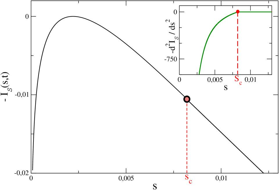
Figure 1: Rate function $-I_{\cal S}(s,t)$ for the sample variance. Parameters $\mu_{k}=2,t=2,r=1,T_{I}=1,T_{F}=0.2$, $d=3$. In the inset the second derivative is shown.

As it suggested by the twofold expression (28) of the saddle point solution, and how it will be explicitly shown in Sec. III.3, $I_{\cal S}$ is singular at $s=s_{C}(t)$. The treatment above clearly shows that the mechanism whereby the singularity is built is a condensation transition, in analogy with the case of the BEC. As already discussed, the difference with BEC is that here condensation is not observed as a typical event but in the fluctuation of a macrovariable. Let us add that $s_{C}$ corresponds to a very rare fluctuation, since as we will show in the next section $s_{C}(t)$ is much larger than the average value.

III.2 Steepest descent

In this section we discuss in detail the steepest descent evaluation of the integral in Eq. (6).

For $s\leq s_{C}$ the saddle point equation (21) admits a solution $z=z^{*}(s)$.

In the region $s>s_{C}$ the evaluation of the integral for the probability (6) can be done using analytical tools inspired to those developed in BK . Let us consider this integral (with $M=S$ and $J=t$) in the neighbourhood of the origin of the cut extending in the $z$-plane from $z=\rho_{0}$ to $\infty$. Singling out the contribution of the $k=0$ mode Eq. (6) reads

$$P(S,t,V)=\int_{-i\infty}^{i\infty}\frac{dz}{2\pi i}e^{-V[f(z,s,t)]}\sqrt{\frac{\rho_{0}(t)}{\rho_{0}(t)-z}}$$ (29)

with

$$f(z,s,t)=sz+\lambda^{0}_{\cal S}(z,t),$$ (30)

$$\lambda^{0}_{\cal S}(z,t)=\frac{1}{2}\int\frac{d^{d}k}{(2\pi)^{d}}\ln[{1-\rho^{-1}_{k}(t)z}],$$ (31)

and

$$\frac{\partial\lambda^{0}_{\cal S}(z,t)}{\partial z}=-{F}_{{\cal S}}(z,t).$$ (32)

Since $\lambda^{0}_{\cal S}(z,t)$ is analytical in the cut plane, its behaviour in the neighborhood of $\rho_{0}(t)$ can be obtained by analytic continuation of ${F}_{{\cal S}}(z,t)$ and then integration of (32).

By using the representation

$$\frac{1}{\rho_{k}-z}=\int_{0}^{\infty}e^{x(z-\rho_{k})}dx=-\int_{0}^{\infty}e^{x(z-\rho_{0})+x(\rho_{0}-\rho_{k})}dx,$$ (33)

where here and in the following for simplicity we will drop the time dependence in $\rho_{k}(t)$, one can write

$$2F_{\cal S}(z,t)=\frac{\Upsilon_{d}}{(2\pi)^{d}}\int_{0}^{\infty}dkk^{d-1}\int_{0}^{\infty}e^{x\Delta_{z}+x(\rho_{0}-\rho_{k})}dx=\frac{\Upsilon_{d}}{(2\pi)^{d}}\int_{0}^{\infty}dxe^{x\Delta_{z}}\int_{0}^{\infty}k^{d-1}e^{x(\rho_{0}-\rho_{k})}dk,$$ (34)

where $\Delta_{z}=z-\rho_{0}$. Then one has

$$2(2\pi)^{d}F_{\cal S}(z,t)/\Upsilon_{d}\equiv\int_{0}^{\infty}e^{x\Delta_{z}}I(x)dx$$ (35)

with

$$I(x)=\int_{0}^{\infty}k^{d-1}e^{x(\rho_{0}-\rho_{k})}dk.$$ (36)

For $x\gg\frac{2t}{C_{t}}$, where $C_{t}$ is defined in Eq. (26), one has

$$I(x)\simeq\frac{x^{-d/2}\Gamma(d/2)(C_{t})^{-d/2}}{2}.$$ (37)

We now evaluate the derivative $W^{\prime}(\Delta_{z})$ of the quantity $W(\Delta_{z})=\int_{0}^{\infty}e^{x\Delta_{z}}I(x)dx$ on the r.h.s. of Eq. (35). For small $\Delta_{z}$, from Eq. (37) one has $W^{\prime}(\Delta_{z})=A(-\Delta_{z})^{d/2-2}$ where $A=\int_{0}^{\infty}y^{-d/2+1}e^{-y}\frac{\Gamma(d/2)}{2(C_{t})^{d/2}}dy$ for $2<d<4$. Then $W(\Delta_{z})$ can be calculated by integration and Eq.(35) becomes

$$F_{\cal S}(z,t)=s_{C}-\frac{\Upsilon_{d}A}{(2\pi)^{d}(d-2)}(-\Delta_{z})^{d/2-1},$$ (38)

where $s_{c}$ is a shorthand for $s_{C}(t)$. Therefore in the neighborhood of $\rho_{0}$ the derivative of $f(z,s,t)$ can be written as

$$f^{\prime}(z,s,t)=s-s_{C}+\frac{\Upsilon_{d}A}{(2\pi)^{d}(d-2)}(\rho_{0}-z)^{d/2-1}$$ (39)

and hence

$$f(z,s,t)=f(\rho_{0},s,t)+(s-s_{C})(z-\rho_{0})+K(\rho_{0}-z)^{d/2}$$ (40)

where $K=-\frac{2\Upsilon_{d}A}{(2\pi)^{d}d(d-2)}<0$. The above expansion shows that the integrand in Eq.(29) always has a saddle point at $z=\rho_{0}$ if $s>s_{C}$, namely the statement of Eq. (28), with the steepest descent contour having a cusp in $z=\rho_{0}$. Hence the dominant contribution to the integral in Eq. (29) can be now evaluated as

$$P(S,t,V) = \frac{e^{-Vf(\rho_{0},s,t)}\sqrt{\rho_{0}}}{2\pi i}\int_{-i\infty}^{i\infty}\frac{e^{V(s-s_{C})(\rho_{0}-z)}}{(\rho_{0}-z)^{1/2}}dz=e^{-Vf(\rho_{0},s,t)}\sqrt{\frac{\rho_{0}}{\pi V(s-s_{C})}}$$ (41)

$$= \sqrt{\frac{\rho_{0}}{\pi V(s-s_{C})}}\,e^{-V\rho_{0}[\lambda^{0}_{\cal S}(\rho_{0},t)+s]},$$

where the integral representation of the $\Gamma$-function has been used. This shows that the rate function is linear in $s$, as it is clear from Eq. (9) (with $m=s$) when $z^{*}$ is independent on $s$.

III.3 Singularity

The previous calculation shows that there is singularity (the marked dot in Fig. 1) located at $s=s_{C}$ in the rate function.

In order to analyze the nature of such singularity we will compute $s$-derivatives of the rate function on the right and on the left of $s_{C}$, and then take the limit for $s\to s_{C}^{\pm}$. Starting with the sector $s>s_{C}$, due to the sticking $z^{*}=\rho_{0}$ of the saddle point solution, from Eq. (30) one has

$${\frac{df(z^{*}(s),s,t)}{ds}}=\rho_{0}$$ (42)

while all right derivatives of higher order are zero.

On the other hand, for $s<s_{C}$, using Eqs. (30,32) one has

$${\frac{df(z^{*}(s),s,t)}{ds}}=\left[z+z^{\prime}(s-F_{\cal S}(z,t))\right]_{z=z^{*}(s)}=z|_{z=z^{*}(s)}=z^{*}(s),$$ (43)

where $z^{\prime}=dz(s)/ds$ and we have used the saddle point equation (21). For $s\to s_{c}$, $z\to\rho_{0}$ and this left derivative equals the right one (42). The second left derivative is given by

$$\left.{\frac{d^{2}f(z^{*}(s),s,t)}{ds^{2}}}\right|_{s_{C}^{-}}=\left.z^{\prime}\right|_{z=z^{*}(s)}.$$ (44)

Near $s_{C}$, for $z\to\rho_{0}$, using Eqs. (21,38) one has that $z^{\prime}|_{z=z^{*}(s)}$ goes to zero as $(\rho_{0}-z)^{2-d/2}$ for $d<4$. Hence the second left derivative vanishes and equals the right one at $s=s_{C}$. This is shown in the inset of Fig. 1. This figure shows that the second derivative has a kink at $s=s_{C}$, as it can be shown by considering the third left derivative, which reads

$${\frac{d^{3}f(z^{*}(s),s,t)}{ds^{3}}}=z^{\prime\prime}|_{z=z^{*}(s)}.$$ (45)

Using again Eqs. (21,38) for $s$ near $s_{C}$ one has $\frac{d^{3}f(z^{*}(s),s,t)}{ds^{3}}=\frac{-2(2\pi)^{d}(d-4)}{\Upsilon_{d}A^{2}}(\rho_{0}-z)^{3-d}$. Therefore in $d=3$ the large deviation function has a discontinuity on the third derivative at $s=s_{c}$.

III.4 Phase diagram

The critical line $s_{c}(t)$ for $d=3$ is displayed in Fig. 2. In order to understand this phase diagram, one should keep in mind that fixing the value of $s$ amounts to implement a spherical constraint à la Berlin and Kac BK . Let us first consider equilibrium, in the time region $t\leq 0$ preceding the quench. Here, the critical line is horizontal and corresponds to the critical threshold $s_{C}(T_{I})$ of the spherical model at the temperature $T_{I}$.

Consider, next, the relaxation regime after the quench, for $t>0$. Following the discussion in noi , when quenches to a finite final temperature are considered (upper panel of Fig. 2) there are two time regimes separated by the minimum of the critical line, about the characteristic time $\tau\sim r^{-1}$, which is the relaxation time of the slowest mode with $\vec{k}=0$. In the first regime $(0<t<\tau)$ the system is strongly off equilibrium and the threshold $s_{C}(t)$ drops abruptly. In the second regime $(t>\tau)$ the system gradually equilibrates to the final temperature and $s_{C}(t)$ saturates slowly toward the final equilibrium value $s_{C}(T_{F})<s_{C}(T_{I})$. A few observations are in order: i) The plot of the average $\langle s(t)\rangle$ lies below the critical line, showing that condensation of fluctuations is always a rare event. The plot of $[s_{C}(t)-\langle s(t)\rangle]$ shows that the rarity of the condensation event varies with time and that the most favourable time window for condensation is around $\tau$, where the difference is minimized. Hence, condensation of the fluctuations is enhanced by the off equilibrium dynamics. ii) The non-monotonicity of the critical line is a remarkable dynamical feature, leading to a re-entrance phenomenon. Namely, when the transition is driven by $t$, and $s$ is kept fixed to a value in between $s_{C}(T_{F})$ and $s_{C}(T_{I})$, a fluctuation of this size at first is normal and then condenses, while for $s$ in between the minimum of the critical line and $s_{C}(T_{F})$, the fluctuation undergoes a second and reverse transition becoming normal again at late times.

For a quench to $T_{F}=0$, shown in the lower panel of Fig. 2, the critical value in the equilibrium state at the final temperature $s_{C}(T_{F}=0)=0$ vanishes and condensation is asymptotically observed for any allowed value of $s$.

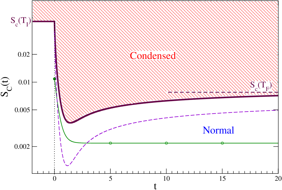
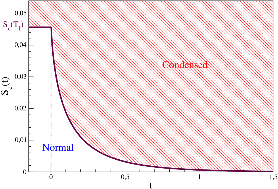
Figure 2: Phase diagram of order parameter sample variance. The upper horizontal dashed line corresponds to $s_{C}(T_{F})$. The green line is the plot of $\langle s(t)\rangle$. The parameters are: $r=1,T_{I}=1,d=3$ and $T_{F}=0.2$ or $T_{F}=0$ in the upper and lower panel respectively. In the upper panel the lower dashed line is the difference $[s_{C}(t)-\langle s(t)\rangle]$.

IV Conclusions

In this paper we have discussed a mechanism whereby a singularity can be produced in the probability distribution $P(M)$ of the fluctuations of a macrovariable ${\cal M}$ in a generic thermodynamic system. We have addressed this problem in the framework of a specific model, the Gaussian model, where analytical calculations can be carried over and the non-analytical behavior can be explicitly exhibited. We have discussed how this phenomenon can be related to the behavior of a dual model obtained from the original one by exerting a constraint. For the Gaussian model considered here, upon choosing ${\cal M}$ as the order-parameter variance ${\cal S}=\varphi^{2}(\vec{x},t)$, the dual model is represented by the Spherical model. Then, at least in equilibrium, the singularity of $P(S)$ can be interpreted as the counterpart of the ferro-paramagnetic phase-transition determined by the spherical constraint. An analogous phenomenon, with a similar interpretation, is observed also out of equilibrium, as we have shown by considering the evolution of the Gaussian model after a temperature quench. The non-analytical behavior observed in this model has been related to the properties of the steepest descent path whose evaluation was carried over explicitly in this paper.

The phenomenon of condensation of fluctuations is not restricted to the Gaussian model neither to the kind of quantities we have considered insofar but is a much more general property. It has been observed, for instance, considering the fluctuations of the heat exchanged by a mean-field model (an attempt to go beyond mean-field was done in CGP ) of a ferromagnet in non-equilibrium conditions and the thermal bath in US . Moreover, in FL the singular behavior of the fluctuations of composite operators whose average yield the correlation and the response function was shown. Finally, although for computational purposes we have considered the case of a non-interacting system, the mechanism whereby the fluctuation spectrum can be related to the properties of a dual system is a general property. An interesting future work, therefore, should be devoted to the investigation of fluctuations in interacting systems.

e-mail addresses - corberi@sa.infn.it, gonnella@ba.infn.it, AntPs@ntu.edu.sg

References

- (1) K. Huang, Statistical Mechanics, John Wiley and Sons, New York 1967
- (2) T. H. Berlin and M. Kac, Phys. Rev. 86, 821 (1952)
- (3) For the condensation transition when the spherical constraint is imposed in the mean via the large limit, see C. Castellano, F. Corberi, and M. Zannetti, Phys. Rev. E 56, 4973 (1997)
- (4) N. Goldenfeld, Lectures on Phase Transitions and the Renormalization Group, Addison-Wesley Publishing Co., Reading, Mass. 1992; P. M. Chaikin and T. C. Lubenski, Principles of Condensed Matter Theory, Cambridge University Press 1995; P. C. Hoenberg and B. I. Halperin, Rev. Mod. Phys. 49, 435 (1977).
- (5) H. Touchette, Phys. Rep. 478, 1 (2009).
- (6) R.J. Harris, A. Rákos, and G.M. Schuetz, J. Stat. Mech. P08003 (2005)
- (7) N. Merhav and Y. Kafri, J. Stat. Mech. P02011 (2010)
- (8) F.Corberi and L.F.Cugliandolo, J. Stat. Mech. P11019 (2012).
- (9) F. Corberi, G. Gonnella, A. Piscitelli and M. Zannetti, J. Phys. A: Math. Theor. 46, 042001 (2013)
- (10) A. Gambassi and A. Silva, Phys. Rev. Lett. 109, 250602 (2012).
- (11) J. Szavits-Nossan, M. R. Evans and S. N. Majumdar, Phys. Rev. Lett. 112, 020602 (2014).
- (12) M. Zannetti, F. Corberi, G. Gonnella arXiv:1404.3975. M. Zannetti, F. Corberi, G. Gonnella and A. Piscitelli, submitted to Communications in Theoretical Physics.
- (13) A. Crisanti and F. Ritort, Europh. Lett. 66, 253 (2004).
- (14) J. R. Gomez-Solano, A. Petrosyan and S. Ciliberto, Phys. Rev. Lett. 106, 200602 (2011)
- (15) C. Godrèche and J. M. Luck, J. Phys. A: Math. Gen. 33, 9141 (2000) F. Corberi, E. Lippiello and M. Zannetti, Phys. Rev. E, 65 046136 (2002); A. Annibale and P. Sollich, J. Phys. A: Math. Gen. 39, 2853 (2006).
- (16) F. Ritort, J. Stat. Mech.: Theory and Experiment, P10016 (2004); B. Derrida, J. Stat. Mech. P07023 (2007); C. Jardina, J. Kurchan and L. Peliti, Phys. Rev. Lett. 96, 120603 (2006); C. Jardina, J. Kurchan, V. Lecomte and J. Tailleur, J. Stat. Phys. 145, 787 (2011).
- (17) D. J. Amit and M. Zannetti, J. Stat. Phys. 7, 31 (1973).
- (18) J. Zinn-Justin, Quantum Field Theory and Critical Phenomena, Chpt. 30, 4th Edition, Clarendon Press, Oxford (2002).
- (19) S. K. Ma, Modern Theory of Critical Phenomena, Chpt. IX, W. A. Benjamin Inc., Reading, Mass. (1976);
- (20) This type of transition was first observed in the fluctuations of the heat exchanged by a ferromagnet quenched below the critical point in Ref. US and in the fluctuations of composite operators whose average are correlation and response functions in Ref. FL .
- (21) F. Corberi, G. Gonnella, A. Piscitelli J. Stat. Mech. (2011) P10022.