Uniqueness and Lipschitz stability of an inverse boundary value problem for time-harmonic elastic waves

Abstract.

We consider the inverse problem of determining the Lamé parameters and the density of a three-dimensional elastic body from the local time-harmonic Dirichlet-to-Neumann map. We prove uniqueness and Lipschitz stability of this inverse problem when the Lamé parameters and the density are assumed to be piecewise constant on a given domain partition.

1. Introduction

We study the inverse boundary value problem for time-harmonic elastic waves. We consider isotropic elasticity, and allow partial boundary data. The Lamé parameters and the density are assumed to be piecewise constants on a given partitioning of the domain. The system of equations describing time-harmonic elastic waves is given by,

(1.1) $$\begin{cases}\operatorname{div}(\mathbb{C}\hat{\nabla}u)+\rho\omega^{2}u=0&\text{in}~{}\Omega\subset\mathbb{R}^{3},\\ u=\psi&\text{on}~{}~{}\partial\Omega,\end{cases}$$

where $\Omega$ is an open and bounded domain with smooth boundary, $\hat{\nabla}u$ denotes the strain tensor, $\hat{\nabla}u:=\frac{1}{2}(\nabla u+(\nabla u)^{T})$, $\psi\in H^{1/2}(\partial\Omega)$ is the boundary displacement or source, and $\mathbb{C}\in L^{\infty}(\Omega)$ denotes the isotropic elasticity tensor with Lamé parameters $\lambda,\mu$:

$$\mathbb{C}=\lambda I_{3}\otimes I_{3}+2\mu\mathbb{I}_{sym},~{}\text{a.e. in}~{}\Omega,$$

where $I_{3}$ is $3\times 3$ identity matrix and $\mathbb{I}_{sym}$ is the fourth order tensor such that $\mathbb{I}_{sym}A=\hat{A}$, $\rho\in L^{\infty}(\Omega)$ is the density, and $\omega$ is the frequency. Here, we make use of the following notation for matrices and tensors: For $3\times 3$ matrices $A$ and $B$ we set $A:B=\sum_{i,j=1}^{3}A_{ij}B_{ij}$ and $\hat{A}=\frac{1}{2}(A+A^{T})$. We assume that

(1.2) $$0<\alpha_{0}\leq\mu\leq\alpha_{0}^{-1},0<\beta_{0}\leq 2\mu+3\lambda\leq\beta_{0}^{-1}~{}\text{a.e. in}~{}\Omega,$$

(1.3) $$0\leq\rho\leq\gamma_{0}^{-1}.$$

The Dirichlet-to-Neumann map, $\Lambda_{\mathbb{C},\rho}$, is defined by

$$\Lambda_{\mathbb{C},\rho}:H^{1/2}(\partial\Omega)\ni\psi\rightarrow(\mathbb{C}\hat{\nabla}u)\nu|_{\partial\Omega}\in H^{-1/2}(\partial\Omega),$$

where $\nu$ is the outward unit normal to $\partial\Omega$. We consider the inverse problem:

determine $$\mathbb{C},\rho \Lambda_{\mathbb{C},\rho}$$ from .

For the static case (that is, $\omega=0$) of our problem, Imanuvilov and Yamamoto [28] proved, in dimension two, a uniqueness result for $C^{10}$ Lamé parameters. In dimension three, Nakamura and Uhlmann [36] proved uniqueness assuming that the Lamé parameters are $C^{\infty}$ and that $\mu$ is close to a positive constant. Eskin and Ralston [24] proved a related result. Global uniqueness of the inverse problem in dimension three assuming general Lamé parametres remains an open problem. Beretta et al. proved the uniqueness when the Lamé parameters are assumed to be piecewise constant. They proved the Lipschitz stability when interfaces of subdomains contain flat parts [14]; later, they extended this result to non-flat interfaces [13]. Alessandrini et al. [2] proved a logarithmic stabilty estimate for the inverse problem of identifying an inclusion, where constant Lamé parameters are different from the background ones.

The key application we have in mind is (reflection) seismology, where Lamé parameters and density need to be recovered from the Dirichlet-to-Neumann map. In actual seismic acquisition, raw vibroseis data are modeled by the Neumann-to-Dirichlet map, the inverse of the Dirichlet-to-Neumann map: The boundary values are given by the normal traction underneath the base plate of a vibroseis and are zero (‘free surface’) elsewhere, while the particle displacement (in fact, velocity) is measured by geophones located in a subset of the boundary (Earth’s surface). The applied signal is essentially time-harmonic (suppressing the sweep); see [7, (2.52)-(2.53)]. (The displacement needs to be measured also underneath the base plate.)

A key complication addressed in this paper is the multiparameter aspect of this inverse problem. For the acoustic waves modeled by the equation

(1.4) $$\nabla\cdot(\gamma\nabla u)+q\omega^{2}u=0,$$

Nachman [35] proved the unique recovery of $\gamma\in C^{2}$ and $q\in L^{\infty}$ with Dirichlet-to-Neumann maps at two different admissible frequencies $\omega_{1},\omega_{2}$. For the optical tomography problem, that is, recovering simultaneously $a>0$ and $c>0$ in the partial differential equation

$$-\nabla\cdot(a\nabla u)+cu=0,$$

from all possible boundary Dirichlet and Neumann pairs, Arridge and Lionheart [5] demonstrated the non-uniqueness for general $a$ and $c$. However, when $a$ is piecewise constant and $c$ is piecewise analytic, Harrach [27] proved the uniqueness of this inverse problem. In this paper, we prove, for our problem, that recovering a higher order coefficient and a lower order coefficient jointly, that are assumed to be piecewise constant, only needs single frequency data also. If we assume $\gamma,q$ to be piecewise constant in (1.4), we can establish the uniqueness with single frequency data, following the methods of proof of this paper.

With the conditional Lipschitz stability which we obtain here, we can invoke iterative methods with guaranteed convergence for local reconstruction, such as the nonlinear Landweber iteration [22] and the nonlinear projected steepest descent algorithm [23] (including a stopping criterion which allows inaccurate data). In reflection seismology, iterative methods for solving inverse problems, casting these into optimization problems, have been collectively referred to as Full Waveform Inversion (FWI) through the use of the adjoint state method. These methods were introduced in this field of application by Chavent [18], Lailly [30] and Tarantola & Valette [42, 41] albeit for scalar waves. An early study of stability in dimension one can be found in Bamberger et al. [8]. Mora [33] developed the adjoint state formulation for the case of elastic waves and carried out computational experiments; Crase et al. [21] then carried out applications to field data. Advantages of using time-harmonic data, following specific workflows, were initially pointed out by Pratt and collaborators [39, 38, 37]; Bunks et al. [17] developed an important insight in the use of strictly finite-frequency data. In recent years, there has been a significant effort in further developing and applying these approaches (with emphasis on iterative Gauss-Newton methods) – in the absence of a notion of (conditional) uniqueness, stability or convergence – often in combination with intuitive strategies for selecting parts of the data. In exploration seismology, we mention the work of Gélis et al. [25], Choi [19], Brossier et al. [15, 16] and Xu & McMechan [44]; in global seismology, we mention the work of Tromp et al. [43] and Fichtner & Trampert [26].

In this paper, we consider piecewise constant Lamé parameters and density of the form

$$\mathbb{C}(x)=\sum_{j=1}^{N}(\lambda_{j}I_{3}\otimes I_{3}+2\mu_{j}\mathbb{I}_{sym})\chi_{D_{j}}(x),\quad\rho(x)=\sum_{j=1}^{N}\rho_{j}\chi_{D_{j}}(x),$$

where the $D_{j}$’s, $j=1,\cdots,N$ are known disjoint Lipschitz domains and $\lambda_{j},\mu_{j},\rho_{j},j=1,\cdots,N$ are unknown constants. We establish uniqueness and a Lipschitz stability estimate of the above mentioned inverse boundary value problem. The method of proof follows the ideas introduced by Alessandrini and Vessella [4] in the study of electrical impedance tomography (EIT) problems. The counterpart for scalar waves, that is, the inverse boundary value problem for the Helmholtz equation, was analyzed by Beretta et al. [10].

The existence and the “blow up” behavior of singular solutions close to a flat discontinuity are utilized in our proof. The quantitative estimate of unique continuation for elliptic systems, which is derived from a three spheres inequality, play an essential role in the procedure. We directly prove a log-type stability estimate for the Lamé parameters and the density combined with alternatingly estimating them along a walkway of subdomains. Uniqueness then follows from the stability estimate. From the restriction that the parameters to be recovered lie in a finite-dimensional space, a Lipschitz stability estimate is obtained.

The paper is organized as follows: In Section 2, we summarize the main results. In Section 3, we construct the singular solutions and establish the unique continuation for the system describing time-harmonic elastic waves. We also prove the Fréchet differentiability of the forward map, $(\mathbb{C},\rho)\to\Lambda_{\mathbb{C},\rho}$. In Section 4, we prove the main result. In Section 5, we give some remarks on the problems of identifying the Lamé parameters given the density, and identifying the density given the Lamé parameters.

2. Main result

2.1. Direct problem

We summarize some results concerning the well-posedness of problem (1.1).

Proposition 2.1.

Let $\Omega$ be a bounded Lipschitz domain in $\mathbb{R}^{3}$, $f\in H^{-1}(\Omega)$ and $g\in H^{1/2}(\partial\Omega)$. Assume that $\lambda,\mu,\rho$ satisfy (1.2) and (1.3). Let $\lambda_{1}^{0}$ be the smallest Dirichlet eigenvalue of the operator $-\operatorname{div}(\mathbb{C}_{0}\hat{\nabla}u)$ in $\Omega$, where $\mathbb{C}_{0}=\frac{\beta_{0}-3\alpha_{0}}{2}I_{3}\otimes I_{3}+2\alpha_{0}\mathbb{I}_{sym}$. Then, for any $\omega^{2}\in(0,\frac{\gamma_{0}\lambda_{1}^{0}}{2}]$, there exists a unique solution of

(2.1) $$\begin{cases}\operatorname{div}(\mathbb{C}\hat{\nabla}u)+\rho\omega^{2}u=f&\text{in}~{}\Omega\subset\mathbb{R}^{3},\\ u=g&\text{on}~{}~{}\partial\Omega,\end{cases}$$

satisfying

(2.2) $$\|u\|_{H^{1}(\Omega)}\leq C(\|g\|_{H^{1/2}(\partial\Omega)}+\|f\|_{H^{-1}(\Omega)}),$$

where $C$ depends on $\alpha_{0}$, $\beta_{0}$, $\gamma_{0}$ and $\lambda_{1}^{0}$.

Proof.

Without loss of generality, we let $g=0$. Indeed, we can always introduce a $w=u-\tilde{g}$ where $\tilde{g}\in H^{1}(\Omega)$ is such that $\tilde{g}=g$ on $\partial\Omega$, which satisfies (2.1) with $g=0$. We recall that

(2.3) $$\lambda_{1}^{0}=\min\left\{\int_{\Omega}\mathbb{C}_{0}\hat{\nabla}u:\hat{\nabla}u\,\Big{|}\,u\in H^{1}(\Omega),\,\|u\|_{L^{2}(\Omega)}=1\right\},$$

and observe that $\mathbb{C}\geq\mathbb{C}_{0}$, that is, $(\mathbb{C}-\mathbb{C}_{0})\hat{A}:\hat{A}\geq 0$ for any $3\times 3$ matrix $A$.

We consider on $H^{1}_{0}(\Omega)$ the bilinear form

$$a(u,v)=\int_{\Omega}\mathbb{C}\hat{\nabla}u:\hat{\nabla}v\mathrm{d}x-\int_{\Omega}\omega^{2}\rho u\cdot v\mathrm{d}x.$$

Then we can write problem (2.1) (for $g=0$) in the weak form,

$$a(u,v)=-\langle f,v\rangle\quad\forall v\in H^{1}_{0}(\Omega).$$

Clearly $a(\cdot,\cdot)$ is continuous. We check now that $a(\cdot,\cdot)$ is coercive. To this aim, we recall the Korn inequality

(2.4) $$\int_{\Omega}|\hat{\nabla}u|^{2}\mathrm{d}x\leq 2\int_{\Omega}|\nabla u|^{2}\mathrm{d}x$$

for any $u\in H^{1}_{0}(\Omega)$ (using the matrix norm, $\left|A\right|^{2}=A:A$ for any $3\times 3$ matrix $A$). Furthermore,

$$a(u,u) = \int_{\Omega}\mathbb{C}\hat{\nabla}u:\hat{\nabla}u\mathrm{d}x-\int_{\Omega}\omega^{2}\rho|u|^{2}\mathrm{d}x$$

$$\geq \int_{\Omega}\mathbb{C}_{0}\hat{\nabla}u:\hat{\nabla}u\mathrm{d}x-\omega^{2}\gamma_{0}^{-1}\int_{\Omega}|u|^{2}\mathrm{d}x$$

$$= \frac{1}{2}\int_{\Omega}\mathbb{C}_{0}\hat{\nabla}u:\hat{\nabla}u\mathrm{d}x+\frac{1}{2}\left\{\int_{\Omega}\mathbb{C}_{0}\hat{\nabla}u:\hat{\nabla}u\mathrm{d}x-2\omega^{2}\gamma_{0}^{-1}\int_{\Omega}|u|^{2}\mathrm{d}x\right\}.$$

By (2.3), the strong convexity of $\mathbb{C}_{0}$, the Korn inequality (2.4) and the Poincaré inequality, we have

$$a(u,u) \geq \frac{\xi_{0}}{4}\int_{\Omega}\left|\nabla u\right|^{2}\mathrm{d}x+\frac{1}{2}\left\{\int_{\Omega}\mathbb{C}_{0}\hat{\nabla}u:\hat{\nabla}u\mathrm{d}x-2\omega^{2}\gamma_{0}^{-1}\int_{\Omega}|u|^{2}\mathrm{d}x\right\}$$

$$\geq \frac{\xi_{0}C_{P}}{4}\|u\|_{H^{1}(\Omega)}^{2}$$

indeed, where $\xi_{0}$ depends on $\alpha_{0}$ and $\beta_{0}$ only and $C_{P}$ is the Poincaré constant of $\Omega$. By the Lax-Milgram lemma there exists a unique solution $u\in H^{1}_{0}(\Omega)$ to problem (2.1), and (2.2) holds. ∎

Remark 2.1.

We note that whenever $\omega$ is not in a particular countable subset of real numbers (the set of eigenfrequencies), Problem (2.1) has a unique solution and estimate (2.2) holds with the constant $C$ depending also on $\omega$.

We let $\Sigma$ be an open portion of $\partial\Omega$. We denote by $H^{1/2}_{co}(\Sigma)$ the space

$$H^{1/2}_{co}(\Sigma):=\{\phi\in H^{1/2}(\partial\Omega)\ |\ \operatorname{supp}~{}\phi\subset\Sigma\}$$

and by $H^{-1/2}_{co}(\Sigma)$ the topological dual of $H^{1/2}_{co}(\Sigma)$. We denote by $\langle\cdot,\cdot\rangle$ the dual pairing between $H^{1/2}_{co}(\Sigma)$ and $H^{-1/2}_{co}(\Sigma)$ based on the $L^{2}(\Sigma)$ inner product. By Proposition 2.1 it follows that for any $\psi\in H^{1/2}_{co}(\Sigma)$ there exists a unique vector-valued function $u\in H^{1}(\Omega)$ that is a weak solution of the Dirichlet problem (1.1). We define the local Dirichlet-to-Neumann map $\Lambda_{\mathbb{C},\rho}^{\Sigma}$ as

$$\Lambda_{\mathbb{C},\rho}^{\Sigma}:H^{1/2}_{co}(\Sigma)\ni\psi\rightarrow(\mathbb{C}\hat{\nabla}u)\nu|_{\Sigma}\in H^{-1/2}_{co}(\Sigma).$$

We have $\Lambda_{\mathbb{C},\rho}=\Lambda_{\mathbb{C},\rho}^{\partial\Omega}$. The map $\Lambda_{\mathbb{C},\rho}^{\Sigma}$ can be identified with the bilinear form on $H^{1/2}_{co}(\Sigma)\times H^{-1/2}_{co}(\Sigma)$,

(2.5) $$\hat{\Lambda}_{\mathbb{C},\rho}^{\Sigma}(\psi,\phi):=\langle\Lambda_{\mathbb{C},\rho}^{\Sigma}\psi,\phi\rangle=\int_{\Omega}(\mathbb{C}\hat{\nabla}u:\hat{\nabla}v-\rho\omega^{2}u\cdot v)\mathrm{d}x,$$

for all $\psi,\phi\in H^{1/2}_{co}(\Sigma)$, where $u$ solves (1.1) and $v$ is any $H^{1}(\Omega)$ function such that $v=\phi$ on $\partial\Omega$. We shall denote by $\|\cdot\|_{\star}$ the norm in $\mathcal{L}(H^{1/2}(\Sigma),H^{-1/2}(\Sigma))$ defined by

$$\|T\|_{\star}=\sup\left\{\langle T\psi,\phi\rangle\ \Big{|}\ \psi,\phi\in H^{1/2}_{co}(\Sigma),\|\psi\|_{H^{1/2}_{co}(\Sigma)}=\|\phi\|_{H^{1/2}_{co}(\Sigma)}=1\right\}.$$

2.2. Notation and definitions

For every $x\in\mathbb{R}^{3}$ we set $x=(x^{\prime},x_{3})$ where $x^{\prime}\in\mathbb{R}^{2}$ and $x_{3}\in\mathbb{R}$. For every $x\in\mathbb{R}^{3}$, $r$ and $L$ positive real numbers we denote by $B_{r}(x)$, $B^{\prime}_{r}(x^{\prime})$ and $Q_{r,L}$ the open ball in $\mathbb{R}^{3}$ centered at $x$ of radius $r$, the open ball in $\mathbb{R}^{2}$ centered at $x^{\prime}$ of radius $r$ and the cylinder $B^{\prime}_{r}(x^{\prime})\times(x_{3}-Lr,x_{3}+Lr)$, respectively; $B_{r}(0)$, $B^{\prime}_{r}(0)$ and $Q_{r,L}(0)$ will be denoted by $B_{r}$, $B^{\prime}_{r}$ and $Q_{r,L}$, respectively. We will also write $\mathbb{R}_{+}^{3}=\{(x^{\prime},x_{3})\in\mathbb{R}^{3}:x_{3}>0\}$, $\mathbb{R}_{-}^{3}=\{(x^{\prime},x_{3})\in\mathbb{R}^{3}:x_{3}<0\}$, $B^{+}_{r}=B_{r}\cap\mathbb{R}^{3}_{+}$, and $B^{-}_{r}=B_{r}\cap\mathbb{R}^{3}_{-}$. For any subset $D$ of $\mathbb{R}^{3}$ and any $h>0$, we let

$$(D)_{h}=\{x\in D\ |\ \operatorname{dist}(x,\mathbb{R}^{3}\setminus D)>h\}.$$

Definition 2.2.

Let $\Omega$ be a bounded domain in $\mathbb{R}^{3}$. We say that a portion $\Sigma\subset\partial\Omega$ is of Lipschitz class with constants $r_{0}>0,L\geq 1$ if for any point $P\in\Sigma$, there exists a rigid transformation of coordinates under which $P=0$ and

$$\Omega\cap Q_{r_{0},L}=\{(x^{\prime},x_{3})\in Q_{r_{0},L}\ |\ x_{3}>\psi(x^{\prime})\},$$

where $\psi$ is a Lipschitz continuous function in $B^{\prime}_{r_{0}}$ such that

$$\psi(0)=0\text{~{}}{and}~{}\|\psi\|_{C^{0,1}(B^{\prime}_{r_{0}})}\leq Lr_{0}.$$

We say that $\Omega$ is of Lipschitz class with constants $r_{0}$ and $L$ if $\partial\Omega$ is of Lipschitz class with the same constants.

2.3. Main assumptions

Let $A,L,\alpha_{0},\beta_{0},\gamma_{0},N$ be given positive numbers such that $N\in\mathbb{N}$, $\alpha_{0}\in(0,1)$, $\beta_{0}\in(0,2)$, $\gamma_{0}\in(0,1)$ and $L>1$. We shall refer to them as the prior data.

In the sequel we will introduce a various constants that we will always denote by $C$. The values of these constants might differ from one another, but we will always have $C>1$.

Assumption 2.1 ([14]).

The domain $\Omega\subset\mathbb{R}^{3}$ is open and bounded with

$$|\Omega|\leq A,$$

and

$$\bar{\Omega}=\cup_{j=1}^{N}\bar{D}_{j},$$

where $D_{j},j=1,\ldots,N$ are connected and pairwise non-overlapping open subdomains of Lipschitz class with constants $1,L$. Moreover, there exists a region, say $D_{1}$, such that $\partial D_{1}\cap\partial\Omega$ contains an open flat part, $\Sigma$, and that for every $j\in\{2,\ldots,N\}$ there exist $j_{1},\ldots,j_{M}\in\{1,\ldots,N\}$ such that

$$D_{j_{1}}=D_{1},\quad D_{j_{M}}=D_{j}$$

and, for every $k=2,\ldots,M$

$$\partial D_{j_{k-1}}\cap\partial D_{j_{k}}$$

contains a flat portion $\Sigma_{k}$ such that

$$\Sigma_{k}\subset\Omega,~{}\text{for all}~{}k=2,\ldots,M.$$

Furthermore, for $k=1,\ldots,M$, there exists $P_{k}\in\Sigma_{k}$ and a rigid transformation of coordinates such that $P_{k}=0$ and

$$\Sigma_{k}\cap Q_{1/3,L}=\{x\in Q_{1/3,L}:x_{3}=0\},$$

$$D_{j_{k}}\cap Q_{1/3,L}=\{x\in Q_{1/3,L}:x_{3}<0\},$$

$$D_{j_{k-1}}\cap Q_{1/3,L}=\{x\in Q_{1/3,L}:x_{3}>0\};$$

here, we set $\Sigma_{1}=\Sigma$. We will refer to $D_{j_{1}},\ldots,D_{j_{M}}$ as a chain of subdomains connecting $D_{1}$ to $D_{j}$. For any $k\in\{1,\ldots,M\}$ we will denote by $n_{k}$ the exterior unit vector to $\partial D_{k}$ at $P_{k}$.

An example of such a domain partition with Lipschitz class subdomains is an unstructured tetrahedral mesh.

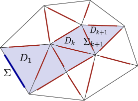
Figure 1. A domain partition including $D_{1}$.

Assumption 2.2.

The stiffness tensor, $\mathbb{C}$, is isotropic and piecewise constant, that is,

$$\mathbb{C}=\sum_{j=1}^{N}\mathbb{C}_{j}\chi_{D_{j}}(x),\quad\mathbb{C}_{j}=\lambda_{j}I_{3}\otimes I_{3}+2\mu_{j}\mathbb{I}_{sym},$$

where the constants $\lambda_{j}$ and $\mu_{j}$ satisfy (cf. (1.2))

(2.6) $$0<\alpha_{0}\leq\mu_{j}\leq\alpha_{0}^{-1},\quad\lambda_{j}\leq\alpha_{0}^{-1},\quad 2\mu_{j}+3\lambda_{j}\geq\beta_{0}>0,\ j=1,\ldots,N.$$

The density, $\rho$, is of the form,

$$\rho=\sum_{j=1}^{N}\rho_{j}\chi_{D_{j}}(x),$$

where the constants $\rho_{j}$ satisfy (cf. (1.3))

$$0\leq\rho_{j}\leq\gamma^{-1}_{0},\ j=1,\ldots,N.$$

Assumption 2.3.

Let $\lambda_{1}^{0}$ be the smallest Dirichlet eigenvalue of operator
$-\operatorname{div}(\mathbb{C}_{0}\hat{\nabla}u)$ in $\Omega$ as before,

$$\omega^{2}\leq\frac{\gamma_{0}\lambda_{1}^{0}}{2}.$$

2.4. Statement of the main result

We define for any set $D\in\mathbb{R}^{3}$,

$$d_{D}((\mathbb{C}^{1},\rho^{1}),(\mathbb{C}^{2},\rho^{2}))=\max\{\|\lambda^{1}-\lambda^{2}\|_{L^{\infty}(D)},\|\mu^{1}-\mu^{2}\|_{L^{\infty}(D)},\|\rho^{1}-\rho^{2}\|_{L^{\infty}(D)}\}.$$

Theorem 2.3.

Let $(\mathbb{C}^{1,2},\rho^{1,2})$ satisfy Assumption 2.2. Let $\Omega$ and $\Sigma$ satisfy Assumption 2.1 and $\omega$ satisfy Assumption 2.3. If $\Lambda_{\mathbb{C}^{2},\rho^{2}}^{\Sigma}=\Lambda_{\mathbb{C}^{1},\rho^{1}}^{\Sigma}$ then $\mathbb{C}^{1}=\mathbb{C}^{2}$ and $\rho^{1}=\rho^{2}$. Moreover, there exists a positive constant $C$ depending on $L$, $A$, $N$, $\alpha_{0}$, $\beta_{0}$, $\gamma_{0}$ and $\lambda_{1}^{0}$ only, such that

(2.7) $$d_{\Omega}((\mathbb{C}^{1},\rho^{1}),(\mathbb{C}^{2},\rho^{2}))\leq C\,\|\Lambda_{\mathbb{C}^{1},\rho^{1}}^{\Sigma}-\Lambda_{\mathbb{C}^{2},\rho^{2}}^{\Sigma}\|_{\star}.$$

In preparation of the proof, we introduce the forward map associated with the inverse problem. We let $\underline{L}:=(\lambda_{1},\ldots,\lambda_{N},\mu_{1},\ldots,\mu_{N},\rho_{1},\ldots,\rho_{N})$ denote a vector in $\mathbb{R}^{3N}$ and $\mathcal{A}$ stand for the open subset of $\mathbb{R}^{3N}$ defined by

(2.8) $$\mathcal{A}:=\!\left\{\underline{L}\in\mathbb{R}^{2N}\ \Big{|}\ \frac{\alpha_{0}}{2}<\mu_{j}<\frac{2}{\alpha_{0}},\lambda_{j}<\frac{2}{\alpha_{0}},2\mu_{j}+3\lambda_{j}>\frac{\beta_{0}}{2},\frac{\gamma_{0}}{2}<\rho_{j}<\frac{2}{\gamma_{0}},j=1,\ldots,N\right\}.$$

For each vector $\underline{L}\in\mathcal{A}$ we can define a piecewise constant stiffness tensor $\mathbb{C}_{\underline{L}}$, and a density $\rho_{\underline{L}}$, with

$$\|\underline{L}\|_{\infty}=\max_{j=1,\ldots,N}\{\sup\{|\lambda_{j}|,\mu_{j},|\rho_{j}|\}\}.$$

The forward map is defined as

(2.9) $$F:\ \mathcal{A}\rightarrow\mathcal{L}(H^{1/2}_{co}(\Sigma),H^{-1/2}_{co}(\Sigma)),\quad\underline{L}\rightarrow F(\underline{L})=\Lambda_{\mathbb{C}_{\underline{L}},\rho_{\underline{L}}}^{\Sigma}.$$

We can identify $F$ with a map $\tilde{F}:\mathcal{A}\rightarrow\mathcal{B}$ upon identifying $\tilde{F}(\underline{L})$ with the bilinear form, $\tilde{\Lambda}_{\mathbb{C}_{\underline{L}},\rho_{\underline{L}}}^{\Sigma}$, on $H^{1/2}_{co}(\Sigma)\times H^{-1/2}_{co}(\Sigma)$ (cf. (2.5)); $\mathcal{B}$ is the Banach space of this bilinear form with the standard norm. In the sequel, we will write $F$ and $\Lambda_{\mathbb{C}_{\underline{L}},\rho_{\underline{L}}}^{\Sigma}$ instead of $\tilde{F}$ and $\tilde{\Lambda}_{\mathbb{C}_{\underline{L}},\rho_{\underline{L}}}^{\Sigma}$. We denote

$$\mathbf{K}:=\{\underline{L}\in\mathcal{A}\ |\ \alpha_{0}\leq\mu_{j}\leq\alpha_{0}^{-1},\lambda_{j}\leq\alpha_{0}^{-1},2\mu_{j}+3\lambda_{j}\geq\beta_{0},0\leq\rho_{j}\leq\gamma_{0}^{-1},j=1,\ldots,N\}.$$

Then the stability estimate in Theorem 2.3 can be stated as follows:

$$\|\underline{L}^{1}-\underline{L}^{2}\|_{\infty}\leq C\|F(\underline{L}^{1})-F(\underline{L}^{2})\|_{\star},$$

for every $\underline{L}^{1},\underline{L}^{2}$ in $\mathbf{K}$. We note that Theorem 2.3 implies that $F$ is injective and that its inverse is Lipschitz continuous.

Remark 2.4.

Assumption 2.3 in Theorem 2.3 can be relaxed to include any $\omega$ that is not in the set of eigenfrequencies. Then the constant $C$ will also depend on the distance between $\omega$ and the set of eigenfrequencies.

3. Preliminary results

Here, we follow Beretta et al. [14, 13]. We summarize the relevant results in their work and adapt them to the time-harmonic problem. We begin this section with Alessandrini’s identity [1, 29]. We let $u_{k}$ be solutions to

$$\operatorname{div}(\mathbb{C}^{k}\hat{\nabla}u_{k})+\rho^{k}\omega^{2}u_{k}=0\quad\text{in}~{}\Omega$$

for $k=1,2$, where $\mathbb{C}^{k},\rho^{k}$ satisfy Assumption 2.2. Then

(3.1) $$\int_{\Omega}\left((\mathbb{C}^{1}-\mathbb{C}^{2})\hat{\nabla}u_{1}:\hat{\nabla}u_{2}-(\rho^{1}-\rho^{2})\omega^{2}u_{1}\cdot u_{2}\right)\mathrm{d}x=\langle(\Lambda_{\mathbb{C}^{1},\rho^{1}}-\Lambda_{\mathbb{C}^{2},\rho^{2}})u_{1},u_{2}\rangle.$$

3.1. Fréchet differentiability of $F$

Here, we prove the Fréchet differentiability of the forward map, $F$.

Proposition 3.1.

Under Assumptions 2.1, 2.2 and 2.3, the map

$$F:\mathcal{A}\rightarrow\mathcal{L}(H^{1/2}_{co}(\Sigma),H^{-1/2}_{co}(\Sigma))$$

is Frechét differentiable in $\mathcal{A}$ and

(3.2) $$\langle DF(\underline{L})[\underline{H}]\psi,\phi\rangle=\int_{\Omega}\left(\mathbb{H}\hat{\nabla}u_{\underline{L}}:\hat{\nabla}v_{\underline{L}}-h\omega^{2}u_{\underline{L}}\cdot v_{\underline{L}}\right)\mathrm{d}x,$$

where $\mathbb{H}=\mathbb{C}_{\underline{H}},h=\rho_{\underline{H}}$. Moreover, $DF:\ \mathcal{A}\rightarrow\mathcal{L}(\mathbb{R}^{3N},\mathcal{L}(H^{1/2}_{co}(\Sigma),H^{-1/2}_{co}(\Sigma)))$ is Lipschitz continuous with Lipschitz constant $C_{DF}$ depending on $A$, $L$, $\alpha_{0}$, $\beta_{0}$, $\gamma_{0}$, $\lambda_{1}^{0}$ only.

Proof.

Fix $\underline{L}\in\mathcal{A}$ and let $\underline{H}\in\mathbb{R}^{3N}$ such that $\|\underline{H}\|_{\infty}$ is sufficiently small. By (3.1) we have

$$\langle(F(\underline{L}+\underline{H})-F(\underline{L}))\psi,\phi\rangle=\int_{\Omega}\mathbb{H}\hat{\nabla}u_{\underline{L}+\underline{H}}:\hat{\nabla}v_{\underline{L}}\mathrm{d}x-\int_{\Omega}h\omega^{2}u_{\underline{L}+\underline{H}}\cdot v_{\underline{L}}\mathrm{d}x.$$

Hence, by setting

(3.3) $$\eta:=\langle(F(\underline{L}+\underline{H})-F(\underline{L}))\psi,\phi\rangle-\int_{\Omega}\mathbb{H}\hat{\nabla}u_{\underline{L}}:\hat{\nabla}v_{\underline{L}}\mathrm{d}x+\int_{\Omega}h\omega^{2}u_{\underline{L}}\cdot v_{\underline{L}}\mathrm{d}x\\ =\int_{\Omega}\mathbb{H}\hat{\nabla}(u_{\underline{L}+\underline{H}}-u_{\underline{L}}):\hat{\nabla}v_{\underline{L}}\mathrm{d}x-\int_{\Omega}h\omega^{2}(u_{\underline{L}+\underline{H}}-u_{\underline{L}})\cdot v_{\underline{L}}\mathrm{d}x,$$

we find that

(3.4) $$|\eta|\leq C\|\underline{H}\|_{\infty}\|\nabla(u_{\underline{L}+\underline{H}}-u_{\underline{L}})\|_{L^{2}(\Omega)}\|\phi\|_{H^{1/2}_{co}(\Sigma)},$$

where $C$ depends on $A,L,\alpha_{0},\beta_{0},\gamma_{0},\lambda_{1}^{0}$ only. We estimate $\|\nabla(u_{\underline{L}+\underline{H}}-u_{\underline{L}})\|_{L^{2}(\Omega)}$. We observe that $w:=u_{\underline{L}+\underline{H}}-u_{\underline{L}}$ is the solution to

(3.5) $$\begin{cases}\operatorname{div}(\mathbb{C}_{\underline{L}}\hat{\nabla}w)+\rho\omega^{2}w=-\text{div}(\mathbb{H}\hat{\nabla}u_{\underline{L}+\underline{H}})-h\omega^{2}u_{\underline{L}+\underline{H}}&\text{in}~{}\Omega,\\ w=0&\text{on}~{}\partial\Omega.\end{cases}$$

By Proposition 2.1, we have

(3.6) $$\begin{split}\|\nabla w\|_{L^{2}(\Omega)}&\leq C\|w\|_{H^{1}(\Omega)}\\ &\leq C\|\text{div}(\mathbb{H}\hat{\nabla}u_{\underline{L}+\underline{H}})\|_{H^{-1}(\Omega)}+C\|h\omega^{2}u_{\underline{L}+\underline{H}}\|_{H^{-1}(\Omega)}\\ &\leq C\|\mathbb{H}\hat{\nabla}u_{\underline{L}+\underline{H}}\|_{L^{2}(\Omega)}+C\|h\omega^{2}u_{\underline{L}+\underline{H}}\|_{H^{-1}(\Omega)}\\ &\leq C\|\underline{H}\|_{\infty}\|u_{\underline{L}+\underline{H}}\|_{H^{1}(\Omega)}+C\|\underline{H}\|_{\infty}\|u_{\underline{L}+\underline{H}}\|_{L^{2}(\Omega)}\\ &\leq C\|\underline{H}\|_{\infty}\|\psi\|_{H^{1/2}_{co}(\Sigma)},\end{split}$$

where $C$ depends on $A,L,\alpha_{0},\beta_{0},\gamma_{0},\lambda_{1}^{0}$. By inserting (3.6) into (3.4) we get

(3.7) $$|\eta|\leq C\|\underline{H}\|^{2}_{\infty}\|\psi\|_{H^{1/2}_{co}(\Sigma)}\|\phi\|_{H^{1/2}_{co}(\Sigma)},$$

that yields (3.2).

We now prove the Lipschitz continuity of $DF$. Let $\underline{L}^{1},\underline{L}^{2}\in\mathcal{A}$ and set

$$\begin{split}\xi:=&\langle(DF(\underline{L}^{2})-DF(\underline{L}^{1}))[\underline{H}]\psi,\phi\rangle\\ =&\int_{\Omega}\left(\mathbb{H}\hat{\nabla}u_{\underline{L}^{2}}:v_{\underline{L}^{2}}-\mathbb{H}\hat{\nabla}u_{\underline{L}^{1}}:v_{\underline{L}^{1}}\right)\mathrm{d}x+\int_{\Omega}\left(h\omega^{2}u_{\underline{L}^{2}}\cdot v_{\underline{L}^{2}}-h\omega^{2}u_{\underline{L}^{1}}\cdot v_{\underline{L}^{1}}\right)\mathrm{d}x\\ =&\int_{\Omega}\mathbb{H}(\hat{\nabla}u_{\underline{L}^{2}}-\hat{\nabla}u_{\underline{L}^{1}}):\hat{\nabla}v_{\underline{L}^{2}}\mathrm{d}x+\int_{\Omega}\mathbb{H}\hat{\nabla}u_{\underline{L}^{1}}:(\hat{\nabla}v_{\underline{L}^{2}}-\hat{\nabla}v_{\underline{L}^{1}})\mathrm{d}x\\ &+\int_{\Omega}h\omega^{2}(u_{\underline{L}^{2}}-u_{\underline{L}^{1}})\cdot v_{\underline{L}^{2}}\mathrm{d}x+\int_{\Omega}h\omega^{2}u_{\underline{L}^{1}}\cdot(v_{\underline{L}^{2}}-v_{\underline{L}^{1}})\mathrm{d}x.\end{split}$$

By reasoning as we did to derive (3.7) we obtain

$$|\xi|\leq C_{DF}\|\underline{H}\|_{\infty}\|\underline{L}^{2}-\underline{L}^{1}\|_{\infty}\|\psi\|_{H^{1/2}_{co}(\Sigma)}\|\phi\|_{H^{1/2}_{co}(\Sigma)},$$

where $C_{DF}$ depends on $A,L,\alpha_{0},\beta_{0},\gamma_{0},\lambda_{1}^{0}$. ∎

3.2. Further notation and definitions

Construction of an augmented domain and extension of $\mathbb{C}$ and $\rho$. First we extend the domain $\Omega$ to a new domain $\Omega_{0}$ such that $\partial\Omega_{0}$ is of Lipschitz class and $B_{1/C}(P_{1})\cap\Sigma\subset\Omega_{0}$, for some suitable constant $C\geq 1$ depending only on $L$. We proceed as in [3]. We set

(3.8) $$\eta_{1}=1/C_{L},\text{where}~{}C_{L}=\frac{3\sqrt{1+L^{2}}}{L},$$

and define, for every $x^{\prime}\in B^{\prime}_{\frac{1}{3}}$

$$\psi^{+}(x^{\prime})=\begin{cases}\frac{\eta_{1}}{2}&\text{for}~{}|x^{\prime}|\leq\frac{\eta_{1}}{4L}\\ \eta_{1}-2L|x^{\prime}|&\text{for}~{}\frac{\eta_{1}}{4L}<|x^{\prime}|\leq\frac{\eta_{1}}{2L}\\ 0&\text{for}~{}|x^{\prime}|>\frac{\eta_{1}}{2L}.\end{cases}$$

We observe that for every $x^{\prime}\in B^{\prime}_{1/3}$, $|\psi^{+}(x^{\prime})|\leq\frac{\eta_{1}}{2}$ and $|\nabla_{x^{\prime}}\psi^{+}(x^{\prime})|\leq 2L$. Next, we denote by

$$D_{0}=\{x=(x^{\prime},x_{3})\in Q_{1/3,L}\ |\ 0\leq x_{3}<\psi^{+}(x^{\prime})\},$$

$$\Omega_{0}=\Omega\cup D_{0}.$$

We have

1. $\Omega_{0}$ has a Lipschitz boundary with constants $\frac{1}{3},3L$;

2. $$\Omega_{0}\supset Q_{1/4LC_{L},L}.$$

Let $\mathbb{C}$ be an isotropic tensor that satisfies Assumption 2.2. We extend $\mathbb{C}$ to $\Omega_{0}$ such that $\mathbb{C}|_{D_{0}}=\mathbb{C}_{0}$. We also extend $\rho$ such that $\rho|_{D_{0}}=1$. Then $\mathbb{C},\rho$ are of the form

(3.9) $$\mathbb{C}=\sum_{j=0}^{N}\mathbb{C}_{j}\chi_{D_{j}}(x),$$

(3.10) $$\rho=\sum_{j=0}^{N}\rho_{j}\ \chi_{D_{j}}(x).$$

Construction of a walkway. We fix $j\in\{1,\ldots,N\}$ and let $D_{j_{1}},\ldots,D_{j_{M}}$ be a chain of domains connecting $D_{1}$ to $D_{j}$. We set $D_{k}=D_{j_{k}}$, $k=1,\ldots,M$. By [3] Proposition 5.5, there exists $C^{\prime}_{L}\geq 1$ depending on $L$ only, such that $(D_{k})_{h}$ is connected for every $k\in\{1,\ldots,M\}$ and every $h\in(0,1/C^{\prime}_{L})$. We introduce

(3.11) $$h_{0}=\min\left\{\frac{1}{6},\frac{1}{C^{\prime}_{L}},\frac{\eta_{1}}{8\sqrt{1+4L^{2}}}\right\}$$

where $\eta_{1}$ is as in (3.8).
Furthermore

1. $Q_{(k)}$, $k=1,\ldots,M$, is the cylinder centered at $P_{k}$ such that by a rigid transformation of coordinates under which $P_{k}=0$ and $\Sigma_{k}$ belongs to the plane $\{(x^{\prime},0)\}$, and $Q_{(k)}=Q_{\eta_{1}/4L,L}$. We also denote $Q^{-}_{(M)}=Q_{(M)}\cap D_{M-1}$;

2. $\mathcal{K}$ is the interior part of the set $\bigcup_{k=1}^{M-1}\bar{D}_{i}$;

3. $\mathcal{K}_{h}=\bigcup_{k=1}^{M-1}(D_{i})_{h}$, for every $h\in(0,h_{0})$;

4. (3.12) $$\tilde{\mathcal{K}}_{h}=\mathcal{K}_{h}\cup Q_{(M)}^{-}\cup\bigcup_{k=1}^{M-1}Q_{(k)};$$

5. $$K_{0}=\left\{x\in D_{0}\ |\ \operatorname{dist}(x,\partial\Omega)>\frac{\eta_{1}}{8}\right\}.$$

It is straightforward to verify that $\tilde{K}_{h}$ is connected and of Lipschitz class for every $h\in(0,h_{0})$ and that

(3.13) $$K_{0}\supset B^{\prime}_{\eta_{1}/4L}(P_{1})\times\left(\frac{\eta_{1}}{8},\frac{\eta_{1}}{4}\right).$$

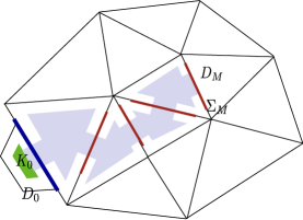
Figure 2. A path or walkway.

3.3. Existence of singular solutions

Next, we construct singular solutions to the system describing time-harmonic elastic waves. We prove the stability estimates for our inverse problems by studying the behavior of singular solutions.

3.3.1. Static fundamental solution in the biphase laminate

In order to construct singular solutions, we make use of special fundamental solutions constructed by Rongved [40] for isotropic biphase laminates. Consider

$$\mathbb{C}_{b}=\mathbb{C}^{+}\chi_{\mathbb{R}^{3}_{+}}+\mathbb{C}^{-}\chi_{\mathbb{R}^{3}_{-}},$$

where $\mathbb{C}^{+}$ and $\mathbb{C}^{-}$ are constant isotropic stiffness tensors given by

$$\mathbb{C}^{+}=\lambda I_{3}\otimes I_{3}+2\mu\mathbb{I}_{sym},~{}~{}\mathbb{C}^{-}=\lambda^{\prime}I_{3}\otimes I_{3}+2\mu^{\prime}\mathbb{I}_{sym},$$

with $\lambda,\mu$ and $\lambda^{\prime},\mu^{\prime}$ satisfying (2.6).

By [40], there exists a fundamental solution $\Gamma:\{(x,y)\ |\ x\in\mathbb{R}^{3},y\in\mathbb{R}^{3},x\neq y\}\rightarrow\mathbb{R}^{3\times 3}$ such that

$$\operatorname{div}(\mathbb{C}_{b}\hat{\nabla}\Gamma(\cdot,y))=-\delta_{y}I_{3}.$$

Here $\delta_{y}$ is the Dirac distribution concentrated at $y$. We point out some properties of $\Gamma$. First of all, it is a fundamental solution, in the sense that $\Gamma(x,y)$ is continuous in $\{(x,y)\in\mathbb{R}^{3}\times\mathbb{R}^{3}\ |\ x\neq y\}$, $\Gamma(x,\cdot)$ is locally integrable in $\mathbb{R}^{3}$ for all $x\in\mathbb{R}^{3}$, and, for every vector valued function $\phi\in C_{0}^{\infty}(\mathbb{R}^{3})$, we have

$$\int_{\mathbb{R}^{3}}\mathbb{C}_{b}\hat{\nabla}\Gamma(\cdot,y):\hat{\nabla}\phi\,\mathrm{d}x=\phi(y).$$

Furthermore, for every $x,y\in\mathbb{R}^{3},x\neq y$, we have

$$|\Gamma(x,y)|\leq\frac{C}{|x-y|}$$

and

$$|\nabla\Gamma(x,y)|\leq\frac{C}{|x-y|^{2}},$$

while for any $r>0$,

(3.14) $$\|\nabla\Gamma(\cdot,y)\|_{L^{2}(\mathbb{R}^{3}\setminus B_{r}(y))}\leq\frac{C}{r^{1/2}},$$

where $C$ depends on $\alpha_{0},\beta_{0}$ only.

3.3.2. Time-harmonic singular solutions

Let $\mathfrak{F}$ denote the union of the flats parts of $\cup_{j=1}^{N}\partial D_{j}$. Let $\mathcal{G}=\cup_{j=0}^{N}\partial D_{j}\setminus\mathfrak{F}$. Let $\mathbb{C}=\sum_{j=0}^{N}\mathbb{C}_{j}\chi_{D_{j}}$ where the tensors $\mathbb{C}_{j}$ satisfy Assumption 2.2. Let $y\in\Omega_{0}\setminus\mathcal{G}$ and let $r=\min(1/4,\text{dist}(y,\mathcal{G}\cup\partial\Omega_{0}))$. Then, in the ball $B_{r}(y)$, either $\mathbb{C}$ is constant, $\mathbb{C}=\mathbb{C}_{j}$ or $\mathbb{C}=\mathbb{C}_{j}+(\mathbb{C}_{j+1}-\mathbb{C}_{j})\chi_{\{x_{3}>a\}}$ for some $a$ with $|a|<r$. We write

$$\mathbb{C}_{y}=\begin{cases}\mathbb{C}_{j}~{}~{}~{}\text{if}~{}\mathbb{C}=\mathbb{C}_{j}~{}\text{in}~{}B_{r}(y),\\ \mathbb{C}_{j}+(\mathbb{C}_{j+1}-\mathbb{C}_{j})\chi_{\{x_{3}>a\}}~{}~{}\text{otherwise},\end{cases}$$

and consider the biphase fundamental solution satisfying

$$\operatorname{div}(\mathbb{C}_{y}\hat{\nabla}\Gamma(\cdot,y))=-\delta_{y}I_{3}~{}\text{in}~{}~{}\mathbb{R}^{3}.$$

Proposition 3.2.

Let $\Omega_{0}$, $\mathbb{C}$ and $\omega$ satisfy Assumptions 2.1, 2.2 and 2.3. Then, for $y\in\Omega_{0}\setminus\mathcal{G}$, there exists only one function $G(\cdot,y)$, which is continuous in $\Omega\setminus\{y\}$, such that

(3.15) $$\int_{\Omega_{0}}\left(\mathbb{C}\hat{\nabla}G(\cdot,y):\hat{\nabla}\phi-\rho\omega^{2}G(\cdot,y)\cdot\phi\right)\mathrm{d}x=\phi(y),~{}~{}\forall\phi\in C^{\infty}_{0}(\Omega_{0}),$$

and

$$G(\cdot,y)=0~{}~{}\text{on}~{}\partial\Omega_{0}.$$

Furthermore, if $\operatorname{dist}(y,\mathcal{G}\cup\partial\Omega_{0})\geq\frac{1}{c_{1}}$ for some $c_{1}>1$ then

(3.16) $$\|G(\cdot,y)-\Gamma(\cdot,y)\|_{H^{1}(\Omega_{0})}\leq C,$$

(3.17) $$\|G(\cdot,y)\|_{H^{1}(\Omega_{0}\setminus B_{r}(y))}\leq Cr^{-1/2},$$

(3.18) $$\|G(\cdot,y)\|_{L^{2}(\Omega_{0})}\leq C,$$

where $C$ depends on $\alpha_{0},\beta_{0},A,L,\gamma_{0},\lambda_{1}^{0}$ and on $c_{1}$.

3.4. Unique continuation for the system describing time-harmonic elastic waves

We state a quantitative estimate of unique continuation. We will omit the proof of this estimate since it is a minor modification of the proof of a similar estimate for the Lamé system of elasticity [14].

Proposition 3.3.

Let $\epsilon_{1},E_{1}$ and $h$ be positive numbers, $h<h_{0}$, where $h_{0}$ is defined in (3.11). Let $v\in H^{1}_{loc}(\mathcal{K})$ be a solution to

$$\operatorname{div}(\mathbb{C}\hat{\nabla}v)+\rho\omega^{2}v=0~{}~{}\text{in}~{}~{}\mathcal{K},$$

such that

$$\|v\|_{L^{\infty}(K_{0})}\leq\epsilon_{1}$$

and

(3.19) $$|v(x)|\leq E_{1}\left(\operatorname{dist}(x,\Sigma_{M})\right)^{-\gamma}~{}~{}\text{for every}~{}x\in\mathcal{K}_{h/2}.$$

Then

(3.20) $$|v(\tilde{x})|\leq Cr^{-3/2-\gamma}\epsilon_{1}^{\tau_{r}}(E_{1}+\epsilon_{1})^{1-\tau_{r}},$$

where $r\in(0,\frac{1}{C})$, $\tilde{x}=P_{M}+rn_{M}$,

$$\tau_{r}=\tilde{\theta}r^{\delta},$$

and $C$, $\delta$ and $\tilde{\theta}$ with $0<\tilde{\theta}<1$ depend on $A$, $L$, $\alpha_{0}$, $\beta_{0}$, $\gamma_{0}$ and $N$.

Therefore, if the solution to the system of time-harmonic elastic waves is small in a subdomain of $\mathcal{K}$, and has a priori bound (3.19), then it is also small in $\mathcal{K}$. The above proposition gives a quantitative estimates on how the smallness propagates.

4. Proof of the main result

In this section we prove the main result that consists of showing the uniform continuity for $DF$ and $F^{-1}$, and establishing a lower bound for $DF$. These results together with the Fréchet differentiability of $F$ establish Theorem 2.3 by Proposition 5 of [6].

4.1. Injectivity of $F|_{\mathbf{K}}$ and uniform continuity of $(F|_{\mathbf{K}})^{-1}$

Let

(4.1) $$\sigma(t)=\begin{cases}|\log t|^{-\frac{1}{8\delta}}~{}~{}\text{for}~{}~{}0<t<\frac{1}{e}\\ t-\frac{1}{e}+1~{}~{}\text{for}~{}~{}t\geq\frac{1}{e}\end{cases}$$

and

$$\sigma_{1}(t)=(\sigma(t))^{1/5}.$$

Theorem 4.1.

For every $\underline{L}^{1},\underline{L}^{2}\in\mathbf{K}$ the following inequality holds true,

(4.2) $$\|\underline{L}^{1}-\underline{L}^{2}\|_{\infty}\leq C_{*}\sigma_{1}^{N}(\|F(\underline{L}^{1})-F(\underline{L}^{2})\|_{\star})$$

where $C_{*}$ is a constant depending on $A,L,\alpha_{0},\beta_{0},\gamma_{0},\lambda_{1}^{0},N$.

Let $j\in\{1,\ldots,N\}$ be such that

$$d_{D_{j}}((\mathbb{C}_{\underline{L}^{1}},\rho_{\underline{L}^{1}}),(\mathbb{C}_{\underline{L}^{2}},\rho_{\underline{L}^{2}}))=d_{\Omega_{0}}((\mathbb{C}_{\underline{L}^{1}},\rho_{\underline{L}^{1}}),(\mathbb{C}_{\underline{L}^{2}},\rho_{\underline{L}^{2}})),$$

and let $D_{j_{1}},\ldots,D_{J_{M}}$ be a chain of domains connecting $D_{1}$ to $D_{j}$. For the sake of simplicity of notation, set $D_{k}=D_{j_{k}}$. Let $\mathcal{W}_{k}=\text{Int}(\cup_{j=0}^{k}\overline{D}_{j})$, $\mathcal{U}_{k}=\Omega_{0}\setminus\mathcal{W}_{k}$, for $k=1,\ldots,M-1$. The stiffness tensors $\mathbb{C}_{\underline{L}^{1}}$ and $\mathbb{C}_{\underline{L}^{2}}$ are extended as in (3.9) to all of $\Omega_{0}$. The densities $\rho_{\underline{L}^{1}}$ and $\rho_{\underline{L}^{2}}$ are extended as in (3.10). We set $\mathbb{C}:=\mathbb{C}_{\underline{L}^{1}}$, $\bar{\mathbb{C}}:=\mathbb{C}_{\underline{L}^{2}}$, $\rho:=\rho_{\underline{L}^{1}}$ and $\bar{\rho}:=\rho_{\underline{L}^{2}}$. Finally, let $\tilde{K}_{k}=\tilde{K}_{h}\cap\mathcal{W}_{k}$ and for $y,z\in\tilde{K}_{k}$ define the matrix-valued function

$$\mathcal{S}_{k}(y,z):=\int_{\mathcal{U}_{k}}\left((\mathbb{C}-\bar{\mathbb{C}})\hat{\nabla}G(x,y):\hat{\nabla}\bar{G}(x,z)-(\rho-\bar{\rho})\omega^{2}G(x,y)\cdot\bar{G}(x,z)\right)\mathrm{d}x,$$

the entries of which are given by

$$\begin{split}&\mathcal{S}_{k}^{(p,q)}(y,z)\\ :=&\int_{\mathcal{U}_{k}}\left((\mathbb{C}-\bar{\mathbb{C}})\hat{\nabla}G^{(p)}(x,y):\hat{\nabla}\bar{G}^{(q)}(x,z)-(\rho-\bar{\rho})\omega^{2}G^{(p)}(x,y)\cdot\bar{G}^{(q)}(x,z)\right)\mathrm{d}x,\end{split}$$

$p,q=1,2,3$, where $G^{(p)}(\cdot,y)$ and $\bar{G}^{(q)}(,z)$ denote respectively the $p$-th columns and the $q$-th columns of the singular solutions corresponding to $\mathbb{C},\rho$ and $\bar{\mathbb{C}},\bar{\rho}$. From (3.17) we have that

$$|\mathcal{S}_{k}^{(p,q)}(y,z)|\leq C(d(y)d(z))^{-1/2}\ \text{for all}\ y,z\in\tilde{\mathcal{K}}_{k},$$

where the constant $C$ depends on the a priori parameters only and $d(y)=d(y,\mathcal{U}_{k})$ and $d(z)=d(z,\mathcal{U}_{k})$.

First, following a similar argument in [14], we have the following two propositions:

Proposition 4.1.

For all $y,z\in\tilde{\mathcal{K}}_{k}$ we have that $\mathcal{S}_{k}^{(\cdot,q)}(\cdot,z)$, $\mathcal{S}_{k}^{(p,\cdot)}(y,\cdot)$, belong to $H^{1}_{loc}(\tilde{\mathcal{K}}_{k})$ and for any $q\in\{1,2,3\}$,

(4.3) $$\operatorname{div}(\mathbb{C}\hat{\nabla}\mathcal{S}_{k}^{(\cdot,q)}(\cdot,z))+\rho\omega^{2}\mathcal{S}_{k}^{(\cdot,q)}(\cdot,z)=0~{}~{}\text{in}~{}\tilde{\mathcal{K}}_{k},$$

and for any $p\in\{1,2,3\}$,

(4.4) $$\operatorname{div}(\bar{\mathbb{C}}\hat{\nabla}\mathcal{S}_{k}^{(p,\cdot)}(y,\cdot))+\bar{\rho}\omega^{2}\mathcal{S}_{k}^{(p,\cdot)}(y,\cdot)=0~{}~{}\text{in}~{}\tilde{\mathcal{K}}_{k}.$$

Proposition 4.2.

If for a positive $\epsilon_{0}$ and for some $k\in\{1,\ldots,M-1\}$

(4.5) $$|\mathcal{S}_{k}(y,z)|\leq\epsilon_{0}~{}\text{for every}~{}(y,z)\in K_{0}\times K_{0},$$

then

(4.6) $$|\mathcal{S}_{k}(y_{r},z_{\bar{r}})|\leq Cr^{-5/2}\bar{r}^{-2}\left(\frac{\epsilon_{0}}{C_{1}+\epsilon_{0}}\right)^{\tau_{r}\tau_{\bar{r}}},$$

where $y_{r}=P_{k+1}+rn_{k+1}$, $z_{\bar{r}}=P_{k+1}+\bar{r}n_{k+1}$, $P_{k+1}\in\Sigma_{k+1}$, $r,\bar{r}\in(0,1/C)$, $\tau_{r}=\bar{\theta}r^{\delta}$, $\tau_{\bar{r}}=\bar{\theta}{\bar{r}}^{\delta}$ and $C,C_{1},\delta,\bar{\theta}\in(0,1)$ depend on $A,L,\alpha_{0},\beta_{0},\gamma_{0}$ only.

We can also prove the following

Proposition 4.3.

If $(\ref{4.5})$ holds, then

(4.7) $$|\partial_{y_{1}}\partial_{z_{1}}\mathcal{S}_{k}(y_{r},z_{\bar{r}})|\leq Cr^{-9/2}\bar{r}^{-3}\left(\frac{\epsilon_{0}}{C_{1}+\epsilon_{0}}\right)^{\tau_{r}\tau_{\bar{r}}},$$

where $y_{r}=P_{k+1}+rn_{k+1}$, $z_{\bar{r}}=P_{k+1}+\bar{r}n_{k+1}$, $P_{k+1}\in\Sigma_{k+1}$, $r,\bar{r}\in(0,1/C)$, $\tau_{r}=\bar{\theta}r^{\delta}$, $\tau_{\bar{r}}=\bar{\theta}{\bar{r}}^{\delta}$ and $C,C_{1},\delta,\bar{\theta}\in(0,1)$ depend on $A,L,\alpha_{0},\beta_{0},\gamma_{0}$ only.

We note that, in the above, $\partial_{y_{1}}$ and $\partial_{z_{1}}$ denote derivatives in directions lying on the interface $\Sigma_{k+1}$.

Proof of Proposition 4.3.

Fix $z\in K_{0}$ and consider the function $v(y):=\mathcal{S}^{(\cdot,q)}(y,z)$, for fixed $q$. By Proposition 4.1 we know that $v$ is a solution of

$$\operatorname{div}(\mathbb{C}\hat{\nabla}v(\cdot))+\rho\omega^{2}v(\cdot)=0~{}~{}\text{in}~{}~{}\tilde{\mathcal{K}}_{k}.$$

Moreover, from Proposition 3.2, we get

$$|v(y)|\leq C_{1}d(y)^{-\frac{1}{2}},~{}~{}y\in\tilde{\mathcal{K}}_{k},$$

where $C_{1}$ depends on $A,L,\alpha_{0},\beta_{0},\gamma_{0},\omega,\lambda_{1}^{0}$. Then, applying Proposition 3.3 for $\epsilon_{1}=\epsilon_{0}$ and $E_{1}=C_{1}$, we have

$$|v(y_{r})|=|\mathcal{S}^{(\cdot,q)}_{k}(y_{r},z)|\leq Cr^{-2}\left(\frac{\epsilon_{0}}{C_{1}+\epsilon_{0}}\right)^{\tau_{r}}$$

for all $y\in B_{r/2}(y_{r})$. By the gradient estimate for an elliptic system (see for example [31]), we obtain

$$|\partial_{y_{1}}v(y_{r})|\leq Cr^{-3}\left(\frac{\epsilon_{0}}{C_{1}+\epsilon_{0}}\right)^{\tau_{r}}.$$

We note that $\partial_{y_{1}}G(x,y_{r})=\partial_{y_{1}}\Gamma_{k+1}(x,y_{r})+\partial_{y_{1}}w(x,y_{r})$, where $\partial_{y_{1}}w(x,y_{r})$ satisfies

$$\begin{cases}\operatorname{div}\left(\mathbb{C}\hat{\nabla}_{x}(\partial_{y_{1}}w(x,y_{r}))\right)+\rho\omega^{2}\partial_{y_{1}}w(x,y_{r})=\operatorname{div}\left((\mathbb{C}_{b}^{k+1}-\mathbb{C})\hat{\nabla}_{x}(\partial_{y_{1}}\Gamma_{k+1}(x,y_{r}))\right)\\ \hphantom{\text{div}\left(\mathbb{C}\hat{\nabla}_{x}(\partial_{y_{1}}w(x,y_{r}))\right)+\rho\omega^{2}\partial_{y_{1}}w(x,y_{r})==}-\rho\omega^{2}\partial_{y_{1}}\Gamma_{k+1}(x,y_{r})\qquad\qquad\text{in}~{}\Omega_{0},\\ \partial_{y_{1}}w(x,y_{r})=-\partial_{y_{1}}\Gamma_{k+1}(x,y_{r})\qquad\qquad\qquad\qquad\qquad\qquad\qquad\qquad\qquad\qquad\text{on}~{}\partial\Omega_{0},\end{cases}$$

where $\Gamma_{k+1}$ is the biphase fundamental solution for stiffness tensor

$$\mathbb{C}_{b}^{k+1}=\mathbb{C}_{k}\chi_{\mathbb{R}^{3}_{+}}+\mathbb{C}_{k+1}\chi_{\mathbb{R}^{3}_{-}}.$$

Thus $\partial_{y_{1}}w(\cdot,y_{r})\in H^{1}(\mathcal{U}_{k})$ and

(4.8) $$\|\partial_{y_{1}}w(\cdot,y_{r})\|_{H^{1}(\mathcal{U}_{k})}\leq C.$$

Moreover,

$$\begin{split}\partial_{y_{1}}v(y_{r})&=\partial_{y_{1}}\mathcal{S}_{k}^{(\cdot,q)}(y_{r},z)\\ &=\int_{\mathcal{U}_{k}}\left((\mathbb{C}-\bar{\mathbb{C}})\hat{\nabla}(\partial_{y_{1}}G(x,y_{r})):\hat{\nabla}\bar{G}(x,z)-(\rho-\bar{\rho})\omega^{2}(\partial_{y_{1}}G(x,y_{r}))\cdot\bar{G}(x,z)\right)\mathrm{d}x,\end{split}$$

while

$$\bar{v}(z)=\partial_{y_{1}}\mathcal{S}_{k}^{(p,\cdot)}(y_{r},z),$$

is a solution to

$$\operatorname{div}(\bar{\mathbb{C}}\hat{\nabla}v(\cdot))+\bar{\rho}\omega^{2}v(\cdot)=0~{}~{}\text{in}~{}~{}\tilde{\mathcal{K}}_{k},$$

by the same reasoning as in Proposition 4.1. By (4.8) and the estimates,

(4.9) $$\|\partial_{y_{1}}\Gamma_{k+1}(\cdot,y)\|_{L^{2}(\mathbb{R}^{3}\setminus B_{r}(y))}\leq Cr^{-1/2},$$

(4.10) $$\|\nabla(\partial_{y_{1}}\Gamma_{k+1}(\cdot,y))\|_{L^{2}(\mathbb{R}^{3}\setminus B_{r}(y))}\leq Cr^{-3/2},$$

we find that

$$|\bar{v}(z)|\leq Cr^{-\frac{3}{2}}d(z)^{-\frac{1}{2}}.$$

Applying Proposition 3.3 with $\epsilon_{1}=r^{-3}\left(\frac{\epsilon_{0}}{C_{1}+\epsilon_{0}}\right)^{\tau_{r}}$ and $E_{1}=Cr^{-\frac{3}{2}}$, we have

$$|\bar{v}(z)|\leq C\bar{r}^{-2}r^{-\frac{9}{2}}\left(\frac{\epsilon_{0}}{C_{1}+\epsilon_{0}}\right)^{\tau_{r}\tau_{\bar{r}}},$$

for all $z\in B_{\bar{r}/2}(z_{\bar{r}})$. Then, again, by the gradient estimate,

$$|\partial_{z_{1}}\bar{v}(z_{\bar{r}})|\leq C\bar{r}^{-3}r^{-\frac{9}{2}}\left(\frac{\epsilon_{0}}{C_{1}+\epsilon_{0}}\right)^{\tau_{r}\tau_{\bar{r}}}.$$

Arguing in a similar way, it also follows that

$$\partial_{z_{1}}\partial_{y_{1}}\mathcal{S}_{k}(y_{r},z_{\bar{r}})=\partial_{z_{1}}\bar{v}(z_{\bar{r}})\\ =\int_{\mathcal{U}_{k}}\Big{(}(\mathbb{C}-\bar{\mathbb{C}})\hat{\nabla}(\partial_{y_{1}}G(x,y_{r})):\hat{\nabla}(\partial_{z_{1}}\bar{G}(x,z_{\bar{r}}))\\ -(\rho-\bar{\rho})\omega^{2}(\partial_{y_{1}}G(x,y_{r}))\cdot(\partial_{z_{1}}\bar{G}(x,z_{\bar{r}}))\Big{)}\mathrm{d}x.$$

This completes the proof of (4.7). ∎

Proof of Theorem 4.1.

We follow a walkway and alternate between estimates for Lamé parameters and for the density. Observe that $\|F(\underline{L}^{1})-F(\underline{L}^{2})\|_{\star}=\|\Lambda_{\mathbb{C},\rho}-\Lambda_{\bar{\mathbb{C}},\bar{\rho}}\|$. We write

$$\epsilon:=\|F(\underline{L}^{1})-F(\underline{L}^{2})\|_{\star}.$$

Then using (3.1), we derive that for every $y,z\in K_{0}$ and for $|l|,|m|=1$,

(4.11) $$\left|\int_{\Omega}\left((\mathbb{C}-\bar{\mathbb{C}})(x)\hat{\nabla}G(x,y)l:\hat{\nabla}\bar{G}(x,z)m-(\rho-\bar{\rho})(x)\omega^{2}G(x,y)l\cdot\bar{G}(x,z)m\right)\mathrm{d}x\right|\leq C\epsilon,$$

where $C$ depends on $\alpha_{0},\beta_{0},\gamma_{0},\omega,A,L$. Let

$$\delta_{k}:=\max_{0\leq j\leq k}\{\max\{|\lambda_{j}-\bar{\lambda}_{j}|,|\mu_{j}-\bar{\mu}_{j}|,|\rho_{j}-\bar{\rho}_{j}|\}\},$$

where $k\in\{0,1,\ldots,M\}$. We will prove that for a suitable, increasing sequence $\{\omega_{k}(\epsilon)\}_{0\leq k\leq M}$ satisfying $\epsilon\leq\omega_{k}(\epsilon)$ for every $k=0,\ldots,M$ we have

$$\delta_{k}\leq\omega_{k}(\epsilon)\Longrightarrow\delta_{k+1}\leq\omega_{k+1}(\epsilon),\text{for every}~{}k=0,\ldots,M-1.$$

Without loss of generality we can choose $\omega_{0}(\epsilon)=\epsilon$. Suppose now that for some $k=\{1,\ldots,M-1\}$ we have

(4.12) $$\delta_{k}\leq\omega_{k}(\epsilon).$$

In the following, we estimate $\delta_{k+1}$ by first estimating $|\lambda_{k+1}-\bar{\lambda}_{k+1}|$, $|\mu_{k+1}-\bar{\mu}_{k+1}|$ and then $|\rho_{k+1}-\bar{\rho}_{k+1}|$. Consider

$$\mathcal{S}_{k}(y,z):=\int_{\mathcal{U}_{k}}\left((\mathbb{C}-\bar{\mathbb{C}})(x)\hat{\nabla}G(x,y):\hat{\nabla}\bar{G}(x,z)-(\rho-\bar{\rho})(x)\omega^{2}G(x,y)\cdot\bar{G}(x,z)\right)\mathrm{d}x,$$

and fix $z\in K_{0}$. From Proposition 3.2 and from (4.11) we get that, for $y,z\in K_{0}$,

$$|\mathcal{S}_{k}(y,z)|\leq C(\epsilon+\omega_{k}(\epsilon)),$$

where $C$ depends on $A,L,\alpha_{0},\beta_{0},\gamma_{0},\lambda_{1}^{0},\omega$. By (4.6) and choosing $\bar{r}=cr$ with $c\in[1/4,1/2]$, we find that there are constants $C_{0},\delta\in(0,1)$ and $\theta_{*}$ depending on $A,L,\alpha_{0},\beta_{0},\gamma_{0},\omega$ and $M$, such that for any $r<1/C_{0}$ and fixed $l,m\in\mathbb{R}^{3}$ with $|l|=|m|=1$,

(4.13) $$|\mathcal{S}_{k}(y_{r},z_{\bar{r}})m\cdot l|\leq Cr^{-9/2}\varsigma\left(\omega_{k}(\epsilon),r\right),$$

where

$$\varsigma(t,s)=\left(\frac{t}{1+t}\right)^{\theta_{*}s^{2\delta}}.$$

We choose $l=m=e_{3}$ and decompose

(4.14) $$\mathcal{S}_{k}(y_{r},z_{\bar{r}})e_{3}\cdot e_{3}=I_{1}+I_{2},$$

where

(4.15) $$I_{1}=\int_{B_{r_{1}}\cap D_{k+1}}\!\!\!\!\Big{(}(\mathbb{C}-\bar{\mathbb{C}})(x)\hat{\nabla}G(x,y_{r})e_{3}:\hat{\nabla}\bar{G}(x,z_{\bar{r}})e_{3}\\ -(\rho-\bar{\rho})(x)\omega^{2}G(x,y_{r})e_{3}\cdot\bar{G}(x,z_{\bar{r}})e_{3}\Big{)}\mathrm{d}x,$$

(4.16) $$I_{2}=\int_{\mathcal{U}_{k+1}\setminus(B_{r_{1}}\cap D_{k+1})}\!\!\!\!\!\!\!\!\!\!\!\!\Big{(}(\mathbb{C}-\bar{\mathbb{C}})(x)\hat{\nabla}G(x,y_{r})e_{3}:\hat{\nabla}\bar{G}(x,z_{\bar{r}})e_{3}\\ -(\rho-\bar{\rho})(x)\omega^{2}G(x,y_{r})e_{3}\cdot\bar{G}(x,z_{\bar{r}})e_{3}\Big{)}\mathrm{d}x,$$

with $r_{1}=\frac{1}{4LC_{L}}$. Then, from Proposition 3.2, we derive immediately that

(4.17) $$|I_{2}|\leq C.$$

By (3.18), we have

$$\left|\int_{B_{r_{1}}\cap D_{k+1}}(\rho-\bar{\rho})(x)\omega^{2}G(x,y_{r})e_{3}\cdot\bar{G}(x,z_{\bar{r}})e_{3}\mathrm{d}x\right|\leq C,$$

where $C$ depends on $A,L,\alpha_{0},\beta_{0},\gamma_{0},\lambda_{1}^{0}$. Using (3.16) and (3.17), we get

(4.18) $$\begin{split}|I_{1}|\geq&\left|\int_{B_{r_{1}}\cap D_{k+1}}(\mathbb{C}^{k+1}_{b}-\bar{\mathbb{C}}^{k+1}_{b})(x)\hat{\nabla}\Gamma_{k+1}(x,y_{r})e_{3}:\hat{\nabla}\bar{\Gamma}_{k+1}(x,z_{\bar{r}})e_{3}\mathrm{d}x\right|-C\left(\frac{1}{\sqrt{r}}+1\right),\\ \end{split}$$

where $\Gamma_{k+1}$ and $\bar{\Gamma}_{k+1}$ are the biphase fundamental solutions introduced in Subsection 3.3 corresponding to the stiffness tensors $\mathbb{C}_{b}^{k+1}$ and $\bar{\mathbb{C}}_{b}^{k+1}$ given by

$$\mathbb{C}_{b}^{k+1}=\mathbb{C}_{k}\chi_{\mathbb{R}^{3}_{+}}+\mathbb{C}_{k+1}\chi_{\mathbb{R}^{3}_{-}},$$

$$\bar{\mathbb{C}}_{b}^{k+1}=\bar{\mathbb{C}}_{k}\chi_{\mathbb{R}^{3}_{+}}+\bar{\mathbb{C}}_{k+1}\chi_{\mathbb{R}^{3}_{-}},$$

up to a rigid coordinate transformation that maps the flat part of $\Sigma_{k+1}$ into $x_{3}=0$. Furthermore by (4.13), (4.14) and (4.17) we obtain

(4.19) $$|I_{1}|\leq C\left(r^{-9/2}\varsigma\left(\omega_{k}(\epsilon),r\right)+1\right),$$

where $C$ depends on $A,L,\alpha_{0},\beta_{0},\gamma_{0},\lambda_{1}^{0}$. Hence, by (4.18) and (4.19) and by performing the change of variables $x=rx^{\prime}$ in the integral, we get

(4.20) $$\left|\int_{B^{-}_{r_{1}/r}}(\mathbb{C}^{k+1}_{b}-\bar{\mathbb{C}}^{k+1}_{b})(x^{\prime})\hat{\nabla}\Gamma_{k+1}(x^{\prime},e_{3})e_{3}:\hat{\nabla}\bar{\Gamma}_{k+1}(x^{\prime},ce_{3})e_{3}\mathrm{d}x^{\prime}\right|\leq\delta_{0}\left(r\right),$$

where

$$\delta_{0}\left(r\right)=C\left[r^{-7/2}\varsigma\left(\omega_{k}(\epsilon),r\right)+r^{1/2}\right].$$

We then follow the procedure of [14] pp. 27-29, and obtain

(4.21) $$|\lambda_{k+1}-\bar{\lambda}_{k+1}|\leq C\sigma(\omega_{k}(\epsilon)),~{}~{}~{}|\mu_{k+1}-\bar{\mu}_{k+1}|\leq C\sigma(\omega_{k}(\epsilon)).$$

Next, we estimate $|\rho_{k+1}-\bar{\rho}_{k+1}|$. By Proposition 4.3, there are constants $C_{0},\delta\in(0,1)$ and $\theta_{*}$ depending on $A,L,\alpha_{0},\beta_{0},\gamma_{0},\omega$ and, increasingly, on $M$, such that for any $r<1/C_{0}$ and fixed $l,m\in\mathbb{R}^{3}$ such that $|l|=|m|=1$,

(4.22) $$|\partial_{y_{1}}\partial_{z_{1}}\mathcal{S}_{k}(y_{r},y_{r})m\cdot l|\leq Cr^{-15/2}\varsigma\left(\omega_{k}(\epsilon),r\right).$$

We choose $l=m=e_{3}$, again, and decompose

(4.23) $$\partial_{y_{1}}\partial_{z_{1}}\mathcal{S}_{k}(y_{r},y_{r})e_{3}\cdot e_{3}=J_{1}+J_{2},$$

where

(4.24) $$J_{1}=\int_{B_{r_{1}}\cap D_{k+1}}\!\!\!\!\!\!\!\!\!\!\!\!\Big{(}(\mathbb{C}-\bar{\mathbb{C}})(x)\hat{\nabla}(\partial_{y_{1}}G(x,y_{r}))e_{3}:\hat{\nabla}(\partial_{z_{1}}\bar{G}(x,y_{r}))e_{3}-\\ -(\rho-\bar{\rho})(x)\omega^{2}(\partial_{y_{1}}G(x,y_{r}))e_{3}\cdot(\partial_{z_{1}}\bar{G}(x,y_{r}))e_{3}\Big{)}\mathrm{d}x,$$

(4.25) $$J_{2}=\int_{\mathcal{U}_{k+1}\setminus(B_{r_{1}}\cap D_{k+1})}\!\!\!\!\!\!\!\!\!\!\!\!\Big{(}(\mathbb{C}-\bar{\mathbb{C}})(x)\hat{\nabla}(\partial_{y_{1}}G(x,y_{r}))e_{3}:\hat{\nabla}(\partial_{z_{1}}\bar{G}(x,y_{r}))e_{3}-\\ -(\rho-\bar{\rho})(x)\omega^{2}(\partial_{y_{1}}G(x,y_{r}))e_{3}\cdot(\partial_{z_{1}}\bar{G}(x,y_{r}))e_{3}\Big{)}\mathrm{d}x.$$

Then, with (4.8), (4.9), (4.10) we derive that

(4.26) $$|J_{2}|\leq C.$$

By estimates (4.8), (4.9), (4.10), and using that $|\lambda_{k}-\bar{\lambda}_{k}|\leq C\omega_{k}(\epsilon)$, $|\mu_{k}-\bar{\mu}_{k}|\leq C\omega_{k}(\epsilon)$, $|\lambda_{k+1}-\bar{\lambda}_{k+1}|\leq C\sigma(\omega_{k}(\epsilon))$ and $|\mu_{k+1}-\bar{\mu}_{k+1}|\leq C\sigma(\omega_{k}(\epsilon))$, we get

(4.27) $$\begin{split}|J_{1}|\geq&\left|\int_{B_{r_{1}}\cap D_{k+1}}(\rho_{k+1}-\bar{\rho}_{k+1})\frac{\partial}{\partial y_{1}}\Gamma_{k+1}(x,y_{r})e_{3}\cdot\frac{\partial}{\partial y_{1}}\Gamma_{k+1}(x,y_{r})e_{3}\mathrm{d}x\right|\\ &-C\left(\frac{1}{\sqrt{r}}+\frac{\sigma(\omega_{k}(\epsilon))}{r^{3}}\right)\\ \geq&|\rho_{k+1}-\bar{\rho}_{k+1}|\int_{B_{r_{1}}\cap D_{k+1}}\left|\frac{\partial}{\partial y_{1}}\Gamma_{k+1}(x,y_{r})e_{3}\right|^{2}\mathrm{d}x-C\left(\frac{1}{\sqrt{r}}+\frac{\sigma(\omega_{k}(\epsilon))}{r^{3}}\right),\end{split}$$

where we have used that

$$\int_{B_{r_{1}}\cap D_{k+1}}\left|\frac{\partial}{\partial y_{1}}\Gamma_{k+1}(x,y_{r})e_{3}\right|\left|\frac{\partial}{\partial y_{1}}\Gamma_{k+1}(x,y_{r})e_{3}-\frac{\partial}{\partial y_{1}}\bar{\Gamma}_{k+1}(x,y_{r})e_{3}\right|\mathrm{d}x\leq C\frac{\sigma(\omega_{k}(\epsilon))}{r}.$$

Furthermore, by (4.22),(4.23) and (4.26) we obtain

(4.28) $$|J_{1}|\leq C\left(r^{-15/2}\varsigma\left(\omega_{k}(\epsilon),r\right)+1\right).$$

By (4.27) and by performing the change of variables $x=rx^{\prime}$ in the integral, we have

$$r^{-1}|\rho_{k+1}-\bar{\rho}_{k+1}|\int_{B^{-}_{r_{1}/r}}\left|\frac{\partial}{\partial y_{1}}\Gamma_{k+1}(x^{\prime},e_{3})e_{3}\right|^{2}\mathrm{d}x^{\prime}\\ \leq C\left(\left(r^{-15/2}\varsigma\left(\omega_{k}(\epsilon),r\right)+1\right)+\frac{1}{\sqrt{r}}+\frac{\sigma(\omega_{k}(\epsilon))}{r^{3}}\right).$$

Since $r_{1}/r\geq C/4LC_{L}$ when $r\in(0,1/C)$, we have

$$\int_{B^{-}_{r_{1}/r}}\left|\frac{\partial}{\partial y_{1}}\Gamma_{k+1}(x^{\prime},e_{3})e_{3}\right|^{2}\mathrm{d}x^{\prime}\geq\int_{B^{-}_{C/4LC_{L}}}\left|\frac{\partial}{\partial y_{1}}\Gamma_{k+1}(x^{\prime},e_{3})e_{3}\right|^{2}\mathrm{d}x^{\prime}\geq C,$$

for some positive $C$. Then

$$|\rho_{k+1}-\bar{\rho}_{k+1}|r^{-1}\leq C\left(\left(r^{-15/2}\varsigma\left(\omega_{k}(\epsilon),r\right)+1\right)+\frac{1}{\sqrt{r}}+\frac{\sigma(\omega_{k}(\epsilon))}{r^{3}}\right),$$

and thus

(4.29) $$|\rho_{k+1}-\bar{\rho}_{k+1}|\leq\delta_{1}(r),$$

where

$$\delta_{1}(r)=C\left[r^{-13/2}\varsigma\left(\omega_{k}(\epsilon),r\right)+\sqrt{r}+\frac{\sigma(\omega_{k}(\epsilon))}{r^{2}}\right].$$

If $\omega_{k}(\epsilon)<1/e$, we choose

$$r=\frac{|\sigma(\omega_{k}(\epsilon))|^{2/5}}{C},$$

and then

(4.30) $$|\rho_{k+1}-\bar{\rho}_{k+1}|\leq C|\sigma(\omega_{k}(\epsilon))|^{1/5}.$$

Otherwise, if $\omega_{k}(\epsilon)\geq 1/e$, since $|\rho_{k+1}-\bar{\rho}_{k+1}|$ is bounded, we get (4.30) trivially. By (4.21) and (4.30), we follow the weakest estimate to get

$$\delta_{k+1}\leq\omega_{k+1}(\epsilon):=C\sigma_{1}(\omega_{k}(\epsilon)).$$

Following the way of alternatingly estimating $|\lambda-\bar{\lambda}|$, $|\mu-\bar{\mu}|$ and $|\rho-\bar{\rho}|$ along the walkay $D_{1},D_{2},\ldots,D_{M}$, and recalling that $\omega_{0}(\epsilon)=\epsilon$, we get (4.2).

∎

The uniqueness statement in Theorem 2.3 is an immediate consequence of the proposition above.

4.2. Injectivity of $DF(\underline{L})$ and estimate from below of $DF|_{\mathbf{K}}$

Proposition 4.4.

Let

$$q_{0}:=\min\{\|DF(\underline{L})[\underline{H}]\|_{\star}\ |\ \underline{L}\in\mathbf{K},\underline{H}\in\mathbb{R}^{3N},\|\underline{H}\|_{\infty}=1\};$$

we have

(4.31) $$(\sigma_{1}^{N})^{-1}(1/C_{\star})\leq q_{0},$$

where $C_{\star}>1$ depends on $A,L,\alpha_{0},\beta_{0},\gamma_{0},\lambda_{1}^{0}$ and $N$ only.

Proof.

By the definition of $q_{0}$ there exists an $\underline{L}_{0}\in\mathbf{K}$ and

$$\underline{H}_{0}=(h_{0,1},\ldots,h_{0,N},k_{0,1},\ldots,k_{0,N},l_{0,1},\ldots,l_{0,N}),~{}~{}\|\underline{H}_{0}\|_{\infty}=1,$$

such that

(4.32) $$\|DF(\underline{L}_{0})[\underline{H}_{0}]\|_{\star}=q_{0}.$$

Therefore, by (3.2), (4.32), we have

(4.33) $$\left|\int_{\Omega}\mathbb{H}(x)\left(\hat{\nabla}G(x,y)l:\hat{\nabla}G(x,z)m-h(x)\omega^{2}G(x,y)l\cdot G(x,z)m\right)\mathrm{d}x\right|\leq Cq_{0}$$

for every $y,z\in\mathcal{K}_{0}$, where $C$ depends on $\alpha_{0},\beta_{0},\gamma_{0},\omega,A,L$, $\mathbb{H}=\mathbb{C}_{\underline{H}_{0}}$, $h=\rho_{\underline{H}_{0}}$ and $G(\cdot,y)$ denotes the singular solution corresponding to $\mathbb{C}_{\underline{L}},\rho_{\underline{L}}$. From now on the vector

$$(0,h_{0,1},\ldots,h_{0,N},0,k_{0,1},\ldots,k_{0,N},0,l_{0,1},\ldots,l_{0,N}),$$

will still be denoted by $\underline{H}_{0}$.

We fix $j\in\{1,\ldots,N\}$ and let $D_{j_{1}},\ldots,D_{j_{M}}$ be a chain of domains connecting $D_{1}$ to $D_{j}$, where

$$\max\{|h_{0,j}|,|k_{0,j}|,|l_{0,j}|\}=\|\underline{H}_{0}\|_{\infty}=1.$$

Now, let

$$\eta_{i}:=\max_{0\leq j\leq i}\{\max\{|h_{0,j}|,|k_{0,j}|,|l_{0,j}|\}\},$$

where $i\in\{0,1,\ldots,M\}$. We will prove that for a suitable increasing sequence $\{\omega_{i}(q_{0})\}_{0\leq i\leq M}$ satisfying $\epsilon\leq\omega_{i}(q_{0})$ for every $k=0,\ldots,M$, we have

$$\delta_{k}\leq\omega_{i}(q_{0})\Longrightarrow\delta_{i+1}\leq\omega_{k+1}(q_{0})\ \text{for every}~{}i=0,\ldots,M-1.$$

Without loss of generality we can choose $\omega_{0}(q_{0})=q_{0}$. Suppose now that for some $i=\{1,\ldots,M-1\}$ we obtain (4.32). Let $\mathcal{Y}_{i}(y,z)=\{\mathcal{Y}_{i}^{(p,q)}(y,z)\}_{1\leq p,q\leq 3}$ be the matrix valued function the elements of which are given by

$$\mathcal{Y}_{i}^{(p,q)}(y,z):=\int_{\mathcal{U}_{i}}\left(\mathbb{H}(x)\hat{\nabla}G^{(p)}(x,y):\hat{\nabla}G^{(q)}(x,z)-h(x)\omega^{2}G^{(p)}(x,y)\cdot G^{(q)}(x,z)\right)\mathrm{d}x,$$

with $z\in K_{0}$ fixed. From Proposition 3.2 and from (4.11) we get that, for $y,z\in K_{0}$,

$$|\mathcal{Y}_{i}(y,z)|\leq C(q_{0}+\omega_{i}(q_{0})),$$

where $C$ depends on $A,L,\alpha_{0},\beta_{0},\gamma_{0},\lambda_{1}^{0}$. Choosing $\bar{r}=cr$ with $c\in[1/4,1/2]$, as in Proposition 4.2, we have that there exists a constant $C_{2}$ such that for every $r\in(0,1/C_{2})$,

(4.34) $$|\mathcal{Y}_{i}(y_{r},z_{\bar{r}})|\leq Cr^{-9/2}\varsigma\left(\omega_{i}(q_{0},r)\right),$$

where

$$\varsigma(t,s)=\left(\frac{t}{1+t}\right)^{\theta_{*}s^{2\delta}}.$$

We choose $l=m=e_{3}$, again, and decompose

(4.35) $$\mathcal{Y}_{k}(y_{r},z_{\bar{r}})e_{3}\cdot e_{3}=I_{1}+I_{2},$$

where

(4.36) $$I_{1}=\int_{B_{r_{1}}\cap D_{i+1}}\left(\mathbb{H}(x)\hat{\nabla}G(x,y_{r})e_{3}:\hat{\nabla}G(x,z_{\bar{r}})e_{3}-h(x)\omega^{2}\bar{G}(x,y_{r})e_{3}\cdot G(x,z_{\bar{r}})e_{3}\right)\mathrm{d}x,$$

(4.37) $$\begin{split}I_{2}=\int_{\mathcal{U}_{i+1}\setminus(B_{r_{1}}\cap D_{i+1})}&\Big{(}\mathbb{H}(x)\hat{\nabla}G(x,y_{r})e_{3}:\hat{\nabla}G(x,z_{\bar{r}})e_{3}\\ &-h(x)\omega^{2}G(x,y_{r})e_{3}\cdot G(x,z_{\bar{r}})e_{3}\Big{)}\mathrm{d}x,\end{split}$$

and $r_{1}=\frac{1}{4LC_{L}}$. Then, from Proposition 3.2, we derive that

(4.38) $$|I_{2}|\leq C.$$

Using (3.18), we find that

$$\left|\int_{B_{r_{1}}\cap D_{k+1}}h(x)\omega^{2}G(x,y_{r})e_{3}\cdot G(x,z_{\bar{r}})e_{3}\mathrm{d}x\right|\leq C,$$

where $C$ depends on $A,L,\alpha_{0},\beta_{0},\gamma_{0},\lambda_{1}^{0}$. Then, by (3.16) and (3.17) we get

(4.39) $$|I_{1}|\geq\left|\int_{B_{r_{1}}\cap D_{i+1}}\mathbb{H}(x)\hat{\nabla}\Gamma_{i+1}(x,y_{r})e_{3}:\hat{\nabla}\Gamma_{i+1}(x,z_{\bar{r}})e_{3}\mathrm{d}x\right|-C\left(\frac{1}{\sqrt{r}}+1\right).$$

With (4.34), (4.35) and (4.38) we obtain

(4.40) $$|I_{1}|\leq C\left(r^{-9/2}\varsigma\left(\omega_{i}(q_{0}),r\right)+1\right),$$

where $C$ depends on $A,L,\alpha_{0},\beta_{0},\gamma_{0},\lambda_{1}^{0}$. Following the procedure of [14] pp. 31-33, we get

(4.41) $$|h_{0,i+1}|\leq C\sigma(\omega_{i}(q_{0})),~{}~{}~{}|k_{0,i+1}|\leq C\sigma(\omega_{i}(q_{0})).$$

Similar to Proposition 4.3, we find that there are constants $C_{2},\delta\in(0,1)$ and $\theta_{*}$ depending on $A,L,\alpha_{0},\beta_{0},\gamma_{0},\omega$ and, increasingly, on $M$, such that for any $r<1/C_{2}$

(4.42) $$|\partial_{y_{1}}\partial_{z_{1}}\mathcal{Y}_{i}(y_{r},y_{r})e_{3}\cdot e_{3}|\leq Cr^{-15/2}\varsigma\left(\omega_{i}(q_{0},r)\right).$$

We decompose

(4.43) $$\partial_{y_{1}}\partial_{z_{1}}\mathcal{Y}_{i}(y_{r},y_{r})e_{3}\cdot e_{3}=J_{1}+J_{2},$$

where

(4.44) $$J_{1}=\int_{B_{r_{1}}\cap D_{i+1}}\Big{(}\mathbb{H}(x)\hat{\nabla}(\partial_{y_{1}}G(x,y_{r}))e_{3}:\hat{\nabla}(\partial_{z_{1}}G(x,y_{r}))e_{3}\\ -h(x)\omega^{2}(\partial_{y_{1}}G(x,y_{r}))e_{3}\cdot(\partial_{z_{1}}G(x,y_{r}))e_{3}\Big{)}\mathrm{d}x,$$

(4.45) $$J_{2}=\int_{\mathcal{U}_{i+1}\setminus(B_{r_{1}}\cap D_{i+1})}\Big{(}\mathbb{H}(x)\hat{\nabla}(\partial_{y_{1}}G(x,y_{r}))e_{3}:\hat{\nabla}(\partial_{z_{1}}G(x,y_{r}))e_{3}\\ -h(x)\omega^{2}(\partial_{y_{1}}G(x,y_{r}))e_{3}\cdot(\partial_{z_{1}}G(x,y_{r}))e_{3}\Big{)}\mathrm{d}x.$$

Using (4.8), (4.9), (4.10) and (4.41), we get

(4.46) $$|J_{2}|\leq C$$

and

(4.47) $$\begin{split}|J_{1}|\geq&\left|\int_{B_{r_{1}}\cap D_{i+1}}l_{0,i+1}\frac{\partial}{\partial y_{1}}\Gamma_{i+1}(x,y_{r})e_{3}\cdot\frac{\partial}{\partial y_{1}}\Gamma_{i+1}(x,y_{r})e_{3}\mathrm{d}x\right|-C\left(\frac{1}{\sqrt{r}}+\frac{\sigma(\omega_{i}(\epsilon))}{r^{3}}\right)\\ =&|l_{0,i+1}|\int_{B_{r_{1}}\cap D_{i+1}}\left|\frac{\partial}{\partial y_{1}}\Gamma_{i+1}(x,y_{r})e_{3}\right|^{2}\mathrm{d}x-C\left(\frac{1}{\sqrt{r}}+\frac{\sigma(\omega_{i}(q_{0}))}{r^{3}}\right).\end{split}$$

Furthermore by (4.42), (4.43) and (4.46), we obtain

(4.48) $$|J_{1}|\leq C\left(r^{-15/2}\varsigma\left(\omega_{i}(q_{0})),r\right)+1\right).$$

Hence, by (4.47) and upon performing the change of variables $x=rx^{\prime}$ in the integral, we obtain

$$r^{-1}|l_{0,i+1}|\int_{B^{-}_{r_{1}/r}}\left|\frac{\partial}{\partial y_{1}}\Gamma_{i+1}(x^{\prime},e_{3})e_{3}\right|^{2}\mathrm{d}x^{\prime}\\ \leq C\left(\left(r^{-15/2}\varsigma\left(\omega_{i}(q_{0})),r\right)+1\right)+\frac{1}{\sqrt{r}}+\frac{\sigma(\omega_{i}(q_{0}))}{r^{3}}\right).$$

Since $r_{1}/r\geq C/4LC_{L}$ when $r\in(0,1/C)$, we have

$$\int_{B^{-}_{r_{1}/r}}\left|\frac{\partial}{\partial y_{1}}\Gamma_{i+1}(x^{\prime},e_{3})e_{3}\right|^{2}\mathrm{d}x^{\prime}\geq\int_{B^{-}_{C/4LC_{L}}}\left|\frac{\partial}{\partial y_{1}}\Gamma_{i+1}(x^{\prime},e_{3})e_{3}\right|^{2}\mathrm{d}x^{\prime}\geq C.$$

Then

$$|l_{0,i+1}|r^{-1}\leq C\left(\left(r^{-15/2}\varsigma\left(\omega_{i}(q_{0})),r\right)+1\right)+\frac{1}{\sqrt{r}}+\frac{\sigma(\omega_{i}(q_{0}))}{r^{3}}\right),$$

and thus

(4.49) $$|l_{0,i+1}|\leq\delta_{1}(r),$$

where

$$\delta_{1}(r)=C\left[r^{-13/2}\varsigma\left(\omega_{i}(q_{0}),r\right)+\sqrt{r}+\frac{\sigma(\omega_{i}(q_{0}))}{r^{2}}\right].$$

If $\omega_{i}(q_{0})<1/e$, we choose

$$r=\frac{|\sigma(\omega_{i}(q_{0}))|^{2/5}}{C}$$

so that

(4.50) $$|l_{0,i+1}|\leq C|\sigma(\omega_{i}(q_{0}))|^{1/5}.$$

Otherwise, if $\omega_{i}(q_{0})\geq 1/e$, because $|l_{0,i+1}|$ is bounded, we get (4.50) trivially. Then, by (4.41) and (4.50) we get

$$\eta_{i+1}\leq\omega_{i+1}(q_{0}):=C\sigma_{1}(\omega_{i}(q_{0})).$$

Finally, by alternating the estimates for $|\lambda-\bar{\lambda}|,|\mu-\bar{\mu}|$ and $|\rho-\bar{\rho}|$, we get

$$1=\eta_{M}\leq C\sigma_{1}^{M}(q_{0})\leq C\sigma_{1}^{N}(q_{0}),$$

and the statement follows. ∎

5. Remarks on two reduced problems

The stability estimates for the following two complementary inverse problems are immediate implications of Theorem 2.3.

1. Inverse Problem S1: For known $\rho$: determine $\mathbb{C}$ from $\Lambda_{\mathbb{C},\rho}$;

2. Inverse Problem S2: For known $\mathbb{C}$: determine $\rho$ from $\Lambda_{\mathbb{C},\rho}$,

However, here, that we get much improved estimates in Theorem 4.1, and Proposition 4.4. This enables us to get better Lipschitz constants in the final Lipschitz stability estimates.

Corollary 5.1.

For every $\underline{L}^{1},\underline{L}^{2}\in\mathbf{K}$ the following inequality holds true

(5.1) $$\|\underline{L}^{1}-\underline{L}^{2}\|_{\infty}\leq C_{*}\sigma^{N}(\|F(\underline{L}^{1})-F(\underline{L}^{2})\|_{\star})$$

if either

$$\rho^{1}_{i}=\rho^{2}_{i},~{}i=1,\cdots,N~{}~{}~{}~{}~{}~{}(\text{Problem S1})$$

or

$$\lambda^{1}_{i}=\lambda^{2}_{i},~{}\mu^{1}_{i}=\mu^{2}_{i},~{}i=1,\cdots,N~{}~{}~{}~{}~{}~{}(\text{Problem S2})$$

where $C_{*}$ is a constant depending on $A,L,\alpha_{0},\beta_{0},\gamma_{0},\lambda_{1}^{0},N$.

Corollary 5.2.

Let

$$q_{0}:=\min\{\|DF(\underline{L})[\underline{H}]\|_{\star}|\underline{L}\in\mathbf{K},\underline{H}\in\mathbb{R}^{3N},\|\underline{H}\|_{\infty}=1\}.$$

We have

(5.2) $$q_{0}\geq(\sigma^{N})^{-1}(1/C_{\star})$$

if either

$$l_{i}=0,~{}i=1,\cdots,N~{}~{}~{}~{}~{}~{}(\text{Problem S1})$$

or

$$h_{i}=k_{i}=0,~{}i=1,\cdots,N~{}~{}~{}~{}~{}~{}(\text{Problem S2})$$

where $C_{\star}>1$, depends on $A,L,\alpha_{0},\beta_{0},\gamma_{0},\lambda_{1}^{0}$ and $N$ only.

We note that, here, $\sigma$ replaces $\sigma_{1}$ in the corollaries above. This is due to the fact that we are not dealing with the multi-parameter identification. That is, we do not need to alternatingly estimate coefficients of different order terms.

References

- [1] G. Alessandrini, Stable determination of conductivity by boundary, Applicable Analysis 27 (1988), 153-172.
- [2] G. Alessandrini, M. di Cristo, A. Morassi, E. Rosset, Stable determination of an inclusion in an elastic body by boundary measurements, SIAM J. Math. Anal. 46 (2014), 2692–-2729.
- [3] G. Alessandrini, L. Rondi, E. Rosset, S. Vessella, The stability for the Cauchy problem for elliptic equations, Inverse Problems 25 (2009), 1–47.
- [4] G. Alessandrini, S. Vessella, Lipschitz stability for the inverse conductivity problem, Adv. Appl. Math. 35 (2005), 207–-241.
- [5] S. Arridge and W. Lionheart, Nonuniqueness in diffusion-based optical tomography, Opt. Lett., 23 ( 1998), no. 11: 882–884.
- [6] V. Bacchelli, S. Vessella, Lipschitz stability for a stationary 2D inverse problem with unknown polygonal boundary, Inverse Problems 22 (2006), 16271658.
- [7] G. Baeten, Theoretical and practical aspects of the vibroseis method, PhD Thesis (1989), Technische Universiteit Delft.
- [8] A. Bamberger, G. Chavent, P. Lailly, About the stability of the inverse problem in 1-D wave equations — application to the interpretation of seismic profiles, Applied Mathematics and Optimization 5 (1979), 1-47.
- [9] E. Beretta, E. Bonnetier, E, Francini, A. Mazzucato, An asymptotic formula for the displacement field in the presence of small anisotropic elastic inclusion, Inverse Problems and Imaging 6 (2012), 1–23.
- [10] E. Beretta, M. V. de Hoop, L. Qiu, Lipschitz stability of an inverse boundary value problem for a Schrödinger type equation, SIAM J. Math. Anal. 45 (2013), no. 2, 679–-699.
- [11] E. Beretta, M. V. de Hoop, L. Qiu, O. Scherzer, Inverse boundary value problem for the helmholtz equation with multi-frequency data, preprint.
- [12] E. Beretta, E. Francini, Lipschitz stability for the impedance tomography problem. The complex case, Comm. PDE. 36 (2011), 1723-1749.
- [13] E. Beretta, E. Francini, A. Morassi, E. Rosset, S. Vessella, Lipschitz continuous dependence of piecewise constant Lamé coefficients from boundary data: the case of non flat interfaces, Inverse Problems 30 (2014), 125005.
- [14] E. Beretta, E. Francini, S. Vessella, Uniqueness and Lipschitz stability for the identification of Lamé parameters from boundary measurements, (2013), preprint,.
- [15] R. Brossier, S. Operto, J. Virieux, Seismic imaging of complex onshore structures by 2D elastic frequency-domain full-waveform inversion, Geophysics 74 (2009), no. 6, WCC105-WCC118.
- [16] R. Brossier, S. Operto, J. Virieux, Which data residual norm for robust elastic frequency-domain full waveform inversion?, Geophysics 75 (2010), no. 3, R37-R46.
- [17] C. Bunks, A. Kurzmann, T. Bohlen, 3D elastic full-waveform inversion of small-scale heterogeneities in transmission, Geophysical Prospecting 61 (1995), no. 6, 1238-1251.
- [18] G. Chavent, Local stability of the output least square parameter estimation technique, Math. Appl. Comp. 2 (1983), 3-22.
- [19] Y. Choi, D. Min, C. Shin, Frequency-domain elastic full waveform inversion using the new pseudo-Hessian matrix: Experience of elastic Marmousi-2 synthethic data, Bulletin of the Seismological Society of America 98 (2008), 2402-2415.
- [20] J. Colan, G. N. Trytten, Pointwise bounds in the Cauchy problem for elliptic system of partial differential equations, Arch. Ration. Mech. Anal. 22 (1966), 143–152.
- [21] E. Crase, A. Pica, M. Noble, J. McDonald, A. Tarantola, Robust elastic nonlinear waveform inversion: Application to real data, Geophysics 55 (1990), no. 5, 527-538.
- [22] M. V. de Hoop, L. Qiu, O. Scherzer, Local analysis of inverse problems: Hólder stability and iterative reconstruction, Inverse Problems 28 (2012).
- [23] M. V. de Hoop, L. Qiu, O. Scherzer, A convergence analysis of a multi-level projected steepest descent iteration for nonlinear inverse problems in Banach spaces subject to stability constraints, Numer. Math. (2014).
- [24] G. Eskin, J. Ralston, On the inverse boundary value problem for linear isotropic elasticity, Inverse Problems 18 (2002), 907-921.
- [25] C. Gélis, J. Virieux, G. Grandjean, Two-dimensional elastic full waveform inversion using Born and Rytov formulations in the frequency domain, Geophys. J. Int., 168 (2007), no. 2, 605-633.
- [26] A. Fichtner, J. Trampert, Hessian kernels of seismic data functionals based upon adjoint techniques, Geophysical Journal 185 (2011), no. 2, 775-798.
- [27] B. Harrach, On uniqueness in diffuse optical tomography, Inverse problems, 25, 2009, 055010 (14pp).
- [28] O. Imanuvilov, M. Yamamoto, Global uniquenss in inverse boundary value problems for Navier-Stokes equations and Lamé system in two dimensions, (2013), preprint.
- [29] V. Isakov, Inverse problems for partial differential equations, 2nd edn, Springer, (2006).
- [30] P. Lailly, The seismic inverse problem as a sequence of before stack migrations, in Conference on Inverse Scattering: Theory and Application, Society for Industrial and Applied Mathematics, (1983), 206-220.
- [31] Y. Li, L. Nirenberg, Estimates for elliptic systems from compostion materials, Comm. Pure Appl. Math. 56 (2003), 892–925.
- [32] C. Lin, G. Nakamura, J. Wang, Optimal three-ball inequalities and quantitative uniqueness for the Lamé system with Lipschitz coefficients, Duke Math. J. 155 (2010), 189–204.
- [33] P. Mora, Nonlinear two dimensional elastic inversion of multioffset seismic data, Geophysics 52 (1987), 1211-1228.
- [34] A. Morassi, E. Rosset, Stable determination of cavities in elastic bodies, Inverse Problems 20 (2004), 453–480.
- [35] A. Nachman, Reconstructions from boundary measurements, Ann. of Math. 128 (1988), 531-576.
- [36] G. Nakamura, G, Uhlmann, Erratum: Global uniqueness for an inverse boundary value problem arising in elasticity, Invent. Math. 152 (2003), 205-207.(Erratum to Invent. Math. 118 (1994), 457-474.)
- [37] R. Pratt, Seismic waveform inversion in the frequency domain, Part 1: Theory and verification in a physical scale model, Geophysics 64, 888–901, (1999).
- [38] R. Pratt, C. Shin, G. Hicks, Gauss-Newtwon and full Newton methods in frequency-space seismic waveform inversion, Geophys. J. Int. 133 (1996), 341-362.
- [39] R. Pratt, M. Worthington, Inverse theory applied to multi-source cross-hole tomography. part 1: Acoustic wave-equation method, Geophysical Prospecting 38 (1990), 287-310.
- [40] L. Rongved, Force interior to one of two joined semi-infinite solids, Proc. 2nd Midwestern Conf. Solid Mech (1955), 1–13.
- [41] A. Tarantola, Linearized inversion of seismic reflection data, Geophysical Prospecting 32 (1984), 998-1015.
- [42] A. Tarantola, B. Valette, Generalized nonlinear inverse problem solved using the least squares criterion, Reviews of Geophysics and Space Physics 20 (1982), 219-232.
- [43] J. Tromp, C Tape, Q. Liu, Seismic tomography, adjoint methods, time reversal and banaa-doughnut kernels, Geophys. J. Int. 160 (2005), 195-216.
- [44] K. Xu, G. McMechan, 2D frequency-domain elastic full-waveform inversion using time-domain modeling and a multisteplength gradient approach, Geophysics 79 (2014), no. 2, R41-R53.