Renormalization schemes for SFT solutions
Joanna L. Karczmarek and Matheson Longton
Department of Physics and Astronomy
University of British Columbia Vancouver, Canada

In this paper, we examine the space of renormalization schemes compatible with the Kiermaier and Okawa [1] framework for constructing Open String Field Theory solutions based on marginal operators with singular self-OPEs. We show that, due to freedom in defining the renormalization scheme which tames these singular OPEs, the solutions obtained from the KO framework are not necessarily unique. We identify a multidimensional space of SFT solutions corresponding to a single given marginal operator.

1 Introduction

The problem of finding analytic String Field Theory (SFT) solutions corresponding to different boundary CFTs has received plenty of attention in the last few years. There are several different approaches to this problem, including a perturbative approach based on marginal deformations of the boundary CFT, as well as a more general non-perturbative approach based on boundary condition changing (bcc) operators. In much of this work, analytic solutions to SFT are constructed as wedge states with insertions. Operators inserted on the boundary of the wedge state are built using either a marginal operator or a bcc operator, together with ghosts and other universal elements such as the stress energy tensor. The largest technical challenge to be overcome in constructing SFT solutions is due to the generically singular nature of marginal deformation operators and bcc operators: when these operators have singular OPEs, regularization schemes must be introduced. Earliest attempts to construct SFT solutions dealt mainly with finite boundary operators (for example, [2, 3]), but the challenge due to singular operators has been mostly overcome: for marginal operators, in [1, 4], and, for bcc operators, in several recent works, including [5, 6, 7]. Other approaches have also been considered in [8] and [9, 10, 11].

One issue that has not been addressed very much is that of uniqueness of the SFT solutions being constructed. In particular, there is the question of whether different renormalization schemes could result in different SFT solutions. Here, we attempt to study the issue of uniqueness, focusing on the formalism developed in [1]. This is one of the formalisms able to handle a time-dependent singular marginal deformation, such as the time-symmetric rolling tachyon solution generated by an exactly marginal operator $\sqrt{2}\cosh(X^{0}/\sqrt{\alpha^{\prime}})$. Since the SFT solution is built out of renormalized operators, we can ask whether different choices of renormalization schemes will lead to different SFT solutions.

We do uncover a two-parameter family of SFT solutions all corresponding to the same marginal operator and discuss the possibility that more might exist. We do not, at this point, have a clear interpretation of these solutions. Notice that previous numerical studies of the rolling tachyon solutions with regular OPE have not always agreed on coefficients [2, 5, 12], and a few possible explanations for the meaning of those coefficients have been suggested in [13]. If these different solutions are gauge equivalent, our analytic approach might make it easier to demonstrate that fact. Should the solutions, however, prove not to be gauge equivalent, under the equivalence of boundary CFTs and open SFT solutions each of them would correspond to a new boundary CFT.

The structure of this paper is as follows: In section 2 we review the conditions that renormalized operators must meet for the construction of [1] to be valid and provide a description of our initial approach. In section 3 we study the space of all possible renormalization schemes at second order in the deformation parameter. In section 4 we consider the cubic order. In section 5 we consider all orders for a particular two-parameter family of renormalization schemes and prove that all the conditions set out by [1] are satisfied for this family. In section 6 we discuss which of the free parameters present in the renormalization scheme actually affect the SFT solution and how. Finally, we propose the existence of an even larger family of solutions. Appendix C contains the proof of an important technical result necessary to prove the first BRST condition of [1] which was not included in that paper.

2 Setup

The approach taken in [1] starts with a marginal operator $V(t)$ with a self-OPE given by

$$V(t)V(0)\sim\frac{1}{t^{2}}+O(1)$$ (1)

with no $\frac{1}{t}$ term. A deformed boundary condition on the interval $(a,b)$ is achieved by inserting an exponential of the marginal operator integrated between $a$ and $b$, defined in terms of a Taylor series in the deformation parameter $\lambda$:

$$e^{\lambda V(a,b)}=\sum_{n=0}^{\infty}\frac{\lambda^{n}}{n!}V(a,b)^{n}~{},$$ (2)

where

$$V(a,b)^{n}=\left(\int_{a}^{b}dtV(t)\right)^{n}~{}=\int_{(a,b)^{n}}d^{n}t~{}V(t_{1})\ldots V(t_{n})~{}.$$ (3)

Since $V(t)$ has a singular self-OPE, the the above expressions need to be regulated. We will denote the regulated (or renormalized) operators by enclosing them with $[~{}~{}~{}]_{r}$.

In [1], a list of conditions which must be satisfied by the renormalization procedure is given. If these conditions are satisfied, the formal solution constructed in [1] will satisfy the SFT equations of motion and be real; however, different renormalization schemes can possibly lead to different SFT solutions. The main goal of this paper is to examine the space of possible renormalization schemes compatible with the condition required for a real SFT solution. We begin by reviewing the conditions that any renormalization scheme must satisfy to construct a SFT solution using the approach of [1]. These conditions are basically physical conditions which ensure that when $[e^{\lambda V(a,b)}]_{r}$ is inserted on the boundary, the effect is a conformal change of boundary conditions on the interval $(a,b)$, and nothing else.

The first condition ensures that the insertion $[e^{\lambda V(a,b)}]_{r}$ does not modify the boundary conditions away from the interval $(a,b)$. In particular, it requires that when products of operators that are inserted away from each other are renormalized, it is sufficient to renormalize each term separately. In other words, the renormalized operator factorizes for operators with disjoint support. For example:

$$\left[\ldots e^{\lambda_{1}V(a,b)}e^{\lambda_{2}V(c,d)}\ldots\right]_{r}=\left[\ldots e^{\lambda_{1}V(a,b)}\right]_{r}\left[e^{\lambda_{2}V(c,d)}\ldots\right]_{r},~{}\text{for}~{}b<c~{}.$$ (4a)

Further, changing the boundary condition on the interval $$(a,b) (b,c) (a,c)$$ and using the same deformation parameter should be the same as changing the boundary condition on the interval . In other words, renormalization should not spoil factorization of exponentials.

$$\left[\ldots e^{\lambda V(a,c)}\ldots\right]_{r}=\left[\ldots e^{\lambda V(a,b)}e^{\lambda V(b,c)}\ldots\right]_{r}~{}.$$ (4b)

This condition was called the ‘replacement condition’ in [1] to differentiate it from the factorization condition (4a). We we will continue to use this term.
The next two conditions ensure that the resulting boundary condition is conformal. The first condition defines two local (unintegrated) operators $$O_{L} O_{R}$$ and , which play an important role in the solution. We have

$$Q_{B}\left[e^{\lambda V(a,b)}\right]_{r}=\left[e^{\lambda V(a,b)}O_{R}(b)\right]_{r}-\left[O_{L}(a)e^{\lambda V(a,b)}\right]_{r}~{},$$ (4c)

which requires the existence and finiteness of the renormalized operators $$\left[O_{L}(a)e^{\lambda V(a,b)}\right]_{r} \left[e^{\lambda V(a,b)}O_{R}(b)\right]_{r} V O_{L,R} Q_{B}$$ and , implying that the OPE of the marginal operator with is not so singular that it cannot be renormalized within the scheme we choose. The second of these two assumptions expresses the fact that is anti-commuting:

$$Q_{B}\left[O_{L}(a)e^{\lambda V(a,b)}\right]_{r}=-\left[O_{L}(a)e^{\lambda V(a,b)}O_{R}(b)\right]_{r}~{}.\\$$ (4d)

To obtain a real solution, it is important not to violate the reflection symmetry:

$$\left[e^{\lambda\int_{a}^{b}dtV(t)}\right]_{r}=\left[e^{\lambda\int_{a}^{b}dtV(a+b-t)}\right]_{r}~{}$$ (4e)

The last condition is:

$$\left[e^{\lambda V(a,b)}\right]_{r}\text{ and }\left[O_{L}(a)e^{\lambda V(a,b)}\right]_{r}\text{ do not depend on the circumference of the wedge.}$$ (4f)

Therefore, the subtractions involved in renormalizing operators need to depend on the operators being renormalized only, and not on the size of the wedge state on which they are inserted. To achieve this last property, in [1], renormalization took two steps: in the first, the infinities were cancelled by subtracting the two-point function; in the second, the finite part of the two-point function (which depends on the width of the wedge) was compensated for. In contrast, we use the divergent part of the two-point function alone to compensate for the divergence and then study the impact of the finite part on the renormalization scheme, which means that in our approach, (4f) is automatically satisfied.

In addition to these explicitly stated conditions, a very natural condition of translation invariance was also implied in [1].

At this point, it is relevant to ask what classes of operators we need to provide a renormalization scheme for. Clearly, we need to be able to renormalize exponentials and their products. This is done order by order, so operators such as $V(a,b)^{n}$ must be renormalizable. Further, the action of the BRST operator $Q_{B}$ on $V(a,b)$ ($Q_{B}V(t)=\frac{\partial}{\partial t}(cV(t))$) immediately implies that $O_{L}(a)=\lambda cV(a)+{\cal O}(\lambda^{2})$ and $O_{R}(b)=\lambda cV(b)+{\cal O}(\lambda^{2})$. Thus, we must be able to at least write down such operators as $\left[V(a)e^{\lambda V(a,b)}\right]_{r}$. In fact, we will see that this is sufficient: we need to renormalize products of exponentials of integrated operators with possible insertions of a single unintegrated $V$ on either the left, or the right, or both. These operators also arise naturally when derivatives are taken, for example: $\frac{\partial}{\partial a}\left[e^{\lambda V(a,b)}\right]_{r}$.

Once we have decided on the renormalization scheme for $\left[e^{\lambda V(a,b)}\right]_{r}$, derivative operators such as $Q_{B}\left[e^{\lambda V(a,b)}\right]_{r}$ and $\frac{\partial}{\partial a}\left[e^{\lambda V(a,b)}\right]_{r}$ will be fixed. The choice of renormalization scheme for such operators as $\left[V(a)e^{\lambda V(a,b)}\right]_{r}$ can influence the explicit form of operators $O_{R,L}$ and the existence of natural properties such as

$$\frac{\partial}{\partial a}\left[e^{\lambda V(a,b)}\right]_{r}~{}~{}\overset{?}{=}~{}~{}-\left[V(a)e^{\lambda V(a,b)}\right]_{r}~{},$$ (5)

but it does not change $Q_{B}\left[e^{\lambda V(a,b)}\right]_{r}$ or $\frac{\partial}{\partial a}\left[e^{\lambda V(a,b)}\right]_{r}$ themselves. In other words, our choice of renormalization scheme for operators with unintegrated insertions will not affect the SFT solution. However, it does affect the linearity of the renormalization scheme (for example, property (5)).

We then need to ask: do the set of assumptions (4) imply that the renormalization scheme is linear? The answer is that the replacement condition (4e) can be interpreted as a statement about linearity. If we accept that

$$\ldots e^{\lambda V(a,c)}\ldots=\ldots e^{\lambda V(a,b)}e^{\lambda V(b,c)}\ldots$$ (6)

(a statement about the singular operators and not about the renormalization), then the replacement condition seems to be a tautology. Its true meaning is revealed when we rewrite it order by order

$$\frac{1}{n!}\left[V(a,c)^{n}\right]_{r}=\left[\sum_{j=0}^{n}\frac{1}{j!(n-j)!}V(a,b)^{j}V(b,c)^{n-j}\right]_{r}~{}$$ (7a)

and then bring the combinatorial sum outside the renormalization:

$$\frac{1}{n!}\left[V(a,c)^{n}\right]_{r}=\sum_{j=0}^{n}\frac{1}{j!(n-j)!}\left[V(a,b)^{j}V(b,c)^{n-j}\right]_{r}~{}.$$ (7b)

Viewed this way, the replacement condition becomes a nontrivial statement about linearity of the renormalization scheme when applied to the exponentials and their products. We will see that this condition places restrictions on possible renormalization schemes.

Repeated application of the replacement condition implies linearity for all operators of the form $V^{(n_{1})}(a_{1},b_{1})\ldots V^{(n_{k})}(a_{k},b_{k})$ with $a_{1}<b_{1}\leq a_{2}<b_{2}\leq a_{3}\ldots\leq a_{k}<b_{k}$ as long as the lengths $b_{i}-a_{i}$ of the intervals involved are all finite. It also applies to operators with an extra insertion of an unintegrated operator on either the left, the right or both (for example: $V(a_{0})V^{(n_{1})}(a_{1},b_{1})\ldots V^{(n_{k})}(a_{k},b_{k})$ where $a_{0}\leq a_{1}$), but with one restriction: in all the parts of the sum, the unintegrated operator must be inserted at the same point. Therefore, the replacement condition does not imply such linearity properties as (5), which requires that linearity be extended to addition of operators where the unintegrated operator is inserted at different points. Such ‘extended’ linearity holds only for some choices of renormalization schemes involving unintegrated operator insertions. Linearity beyond the replacement condition does not seem necessary to construct the SFT solution, and does not affect the details of this solution. However, it is implicitly assumed in the analysis of conformal properties of the renormalized operator, for example in [4] (for more details, see section 3.3).

Our initial approach to renormalization will be to consider products of integrated operators, regulate them with a cut off by modifying the domain of integration so that all insertions are separated by a minimum distance of $\epsilon$, and introduce counterterms that cancel the divergences when $\epsilon$ approaches zero. We will modify the domain of integration so that the insertions of integrated operators are separated by at least $\epsilon$ from any fixed insertions. We will use the notation $\left(~{}\right)_{\epsilon}$ to denote regulated operators, for example

$$\left(V(a,b)^{2}\right)_{\epsilon} =\int_{a}^{b-\epsilon}dt_{1}\int_{t_{1}+\epsilon}^{b}dt_{2}~{}V(t_{1})V(t_{2})~{}+~{}\int_{a+\epsilon}^{b}dt_{1}\int_{a}^{t_{1}-\epsilon}dt_{2}~{}V(t_{1})V(t_{2})~{},$$ (8a)

$$\left(V(a,b)V(b,c)\right)_{\epsilon} =\int_{a}^{b}dt_{1}\int_{\mathrm{max}(b,t_{1}+\epsilon)}^{c}dt_{2}~{}V(t_{1})V(t_{2})$$ (8b)

and

$$\left(V(a)V(a,b)\right)_{\epsilon} =V(a)~{}\int_{a+\epsilon}^{b}dt~{}V(t)~{},~{}.$$ (8c)

A crucial property of our regularization is that it is linear. To show this, consider the most general operator with $n$ $V$-insertions, $\int_{M}V(t_{1})\ldots V(t_{n})$ where $M$ is some measure on $\mathbb{R}^{n}$. For example, $V(a)V(a,b)^{2}$ is associated with a uniform measure on $\{a\}\times(a,b)\times(a,b)$ (where $\{a\}$ is a point and $(a,b)$ is an interval.) When adding two such operators, we simply add the corresponding measures. The map $A\rightarrow(A)_{\epsilon}$ acts on the measure $M(A)$ associated with $A$ by setting it to zero for any point $(t_{1},\ldots,t_{n})$ such that $|t_{i}-t_{j}|<\epsilon$ and leaving it unchanged otherwise. Denote this map by $U_{\epsilon}:M(A)\rightarrow M(A_{\epsilon})$. Since the action of the map $U_{\epsilon}$ on any given point within a measure depends only on the coordinates of that point, we have that $U_{\epsilon}(M+\tilde{M})=U_{\epsilon}(M)+U_{\epsilon}(\tilde{M})$. Thus, $A\rightarrow(A)_{\epsilon}$ is a linear map for any operator. This linearity property will be important to ensure that our renormalization satisfies the replacement condition.

We should point out that our implementation here differs slightly from [1]. In particular, the $\epsilon$-regularization of the operator $V(a,b)V(b,c)$ in that work was not linear, being equivalent to

$$\left(V(a,b)V(b,c)\right)_{\epsilon}^{\text{KO}}=\int_{a}^{b-\frac{\epsilon}{2}}dt_{1}\int_{b+\frac{\epsilon}{2}}^{c}dt_{2}V(t_{1})V(t_{2})~{}.$$ (9)

The difference between our definition (8b) and the above equation is illustrated in figure 1. This lack of linearity makes it difficult to see whether there exists a complete renormalization scheme consistent with the assumption (4b) using the approach in [1].

(a)

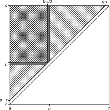
(b)

Figure 1: The regions of integration used in $\left(V(a,b)^{2}\right)_{\epsilon}$ and $\left(V(b,c)^{2}\right)_{\epsilon}$ (diagonal hatching), and the region of $\left(V(a,b)V(b,c)\right)_{\epsilon}$ (cross-hatched): (a) using our prescription for the renormalizations. (b) using the prescription of [1], equation (9). The difference is the gray strips, which are not covered using the latter choice. The dashed line indicates the location of a singularity due to colliding operators.

In the $\epsilon\rightarrow 0$ limit, finite operators can be constructed by canceling the divergences in the regulated operators with counterterms, so that generally $[A]_{r}=(A)_{\epsilon}-\mathrm{counterterms}$. While the divergent part of the counterterms is fixed by the OPEs of the operators in question, the finite part is constrained only by the assumptions (4) and we will see that there is considerable freedom there.

3 Renormalization of operators quadratic in $V$

In this section, we begin to construct a general renormalization scheme, starting with the simplest nontrivial situation: operators quadratic in $V$. We will discuss some (but not all) of the conditions (4). Those we do not discuss in this section will be proved in all generality in section 5.

To start with, setting any other operator insertions aside, consider the operator $V(a)V(a,b)$. The corresponding $\epsilon$-regulated operator has the following behaviour for small $\epsilon$:

$$\left(V(a)V(a,b)\right)_{\epsilon}=\frac{1}{\epsilon}~{}+~{}\text{terms finite when $\epsilon$ goes to zero.}$$ (10)

Therefore, the corresponding renormalized operator can be defined as

$$\left[V(a)V(a,b)\right]_{r}=\lim_{\epsilon\rightarrow 0}\left[\left(V(a)V(a,b)\right)_{\epsilon}~{}-~{}G^{L}_{ab}\right]$$ (11)

where the counterterm $G^{L}_{ab}$ is given by

$$G^{L}_{ab}=\frac{1}{\epsilon}+C^{L}_{b-a}~{}.$$ (12)

Note that, by translation invariance, the counterterm $G^{L}_{ab}$ depends on $a$ and $b$ only through the difference $b-a$. Discussion for $G^{R}_{ab}$ parallels that of $G^{L}_{ab}$.

Now, consider another operator requiring regularization, $V(a,b)^{2}$. We have:

$${{1\over 2}}\left(V(a,b)^{2}\right)_{\epsilon}=\frac{b-a}{\epsilon}+\ln\epsilon~{}+~{}\text{terms finite when $\epsilon$ goes to zero.}$$ (13)

(Our factor of ${{1\over 2}}$ is convenient when evaluating the integral: the two components in definition (8a) are equal to each other and therefore either one of them is equal to ${{1\over 2}}\left(V(a,b)^{2}\right)_{\epsilon}$.) The corresponding renormalized operator is then given by

$$\left[V(a,b)^{2}\right]_{r}=\lim_{\epsilon\rightarrow 0}\left[\left(V(a,b)^{2}\right)_{\epsilon}~{}-~{}2G^{D}_{ab}\right]~{},$$ (14)

where the “double” counterterm $G^{D}_{ab}$ for doubly integrated operators is

$$G^{D}_{ab}=\frac{b-a}{\epsilon}+\ln\epsilon+C^{D}_{b-a}~{}.$$ (15)

By a similar process, we also define

$$\left[V(a,b)V(b,c)\right]_{r}=\lim_{\epsilon\rightarrow 0}\left[\left(V(a,b)V(b,c)\right)_{\epsilon}~{}-~{}G^{E}_{abc}\right]~{},$$ (16)

where $G^{E}_{abc}$ is the “edge” counterterm for operators meeting only at a single shared edge,

$$G^{E}_{abc}=-\ln\epsilon+C^{E}_{c-b,b-a}~{}.$$ (17)

As we have discussed already in section 2, our choice of $C^{L,R}_{ab}$ cannot influence the SFT solution, but the choice of $C^{D}_{b-a}$ and $C^{E}_{c-b,b-a}$ certainly can. We now find restrictions on these finite parts of the counterterms due to the replacement condition (4b) and the more general assumption of linearity.

3.1 Replacement condition (4b)

We begin by using condition (4b) with an insertion of $V(a)$ on the left:

$$\left[V(a)e^{\lambda V(a,c)}\right]_{r}=\left[V(a)e^{\lambda V(a,b)}e^{\lambda V(b,c)}\right]_{r}~{},$$ (18)

which to first order in $\lambda$ implies that

$$\left[V(a)V(a,c)\right]_{r}=\left[V(a)V(a,b)\right]_{r}+\left[V(a)V(b,c)\right]_{r}=\left[V(a)V(a,b)\right]_{r}+V(a)V(b,c)~{}.$$ (19a)

For the last term we have used the factorization condition (4a) to remove the renormalization. Since it is trivially true that

$$\left(V(a)V(a,c)\right)_{\epsilon}=\left(V(a)V(a,b)\right)_{\epsilon}+V(a)V(b,c)~{},$$ (19b)

we obtain that

$$C^{L}_{c-a}=C^{L}_{b-a}=C^{L}~{}.$$ (19c)

The finite part of the counterterm for $\left[V(a)V(a,b)\right]_{r}$ is a constant $C^{L}$ which does not depend on the size of the integration region.

A similar argument, condition (4b) with an integrated operator inserted on the left:

$$\left[e^{\lambda_{1}(a,b)}e^{\lambda V(b,d)}\right]_{r}=\left[e^{\lambda_{1}(a,b)}e^{\lambda V(b,c)}e^{\lambda V(c,d)}\right]_{r}~{},$$ (20)

when expanded to first order in $\lambda$ and $\lambda_{1}$, gives

$$\left[V(a,b)V(b,d)\right]_{r}=\left[V(a,b)V(b,c)\right]_{r}+V(a,b)V(c,d)~{},$$ (21a)

which, together with

$$\left(V(a,b)V(b,d)\right)_{\epsilon}=\left(V(a,b)V(b,c)\right)_{\epsilon}+V(a,b)V(c,d)~{},$$ (21b)

yields

$$C^{E}_{d-b,b-a}=C^{E}_{c-b,b-a}~{}.$$ (21c)

This, together with a similar statement given when the extra integrated operator is inserted on the right, implies that $C^{E}_{c-b,b-a}=C^{E}$ is independent of the values of $a$, $b$ and $c$.

Next, we examine condition (4b) without any extra insertions at second order in $\lambda$:

$$\left[V(a,c)^{2}\right]_{r}=\left[V(a,b)^{2}\right]_{r}+\left[V(b,c)^{2}\right]_{r}+2\left[V(a,b)V(b,c)\right]_{r}.$$ (22a)

Since, as follows trivially from the linearity of $$(\ \cdot\ )_{\epsilon}$$,

$$\left(V(a,c)^{2}\right)_{\epsilon}=\left(V(a,b)^{2}\right)_{\epsilon}+\left(V(b,c)^{2}\right)_{\epsilon}+2\left(V(a,b)V(b,c)\right)_{\epsilon}~{},$$ (22b)

after canceling the $$\epsilon$$-dependent terms, we are left with

$$C^{D}_{c-a}-C^{D}_{c-b}-C^{D}_{b-a}-C^{E}=0~{}.$$ (22c)

Therefore the finite counterterm must be of the form $C^{D}_{\Delta t}=C_{0}+C_{1}\Delta t$, and we must have $C^{E}=-C_{0}$.

At this point, our renormalization scheme is parametrized by 4 parameters: $C_{0}$, $C_{1}$, $C^{R}$ and $C^{L}$. We will see that $C^{R}$ and $C^{L}$ do not affect the eventual SFT solution (and we could have set them to zero without a loss of generality) but that $C_{0}$ and $C_{1}$ do. It is worth mentioning that, at this order, our scheme reproduces that of [1] if we take $C_{1}=0$ and $C_{0}=-1$, though comparison for operators with multiple integration regions is complicated by the discrepancy described in section 2.

3.2 The BRST assumptions (4c) and (4d)

These two assumptions are easily proven at second order in $\lambda$. Throughout this section we will omit the limit $\epsilon\rightarrow 0$, and it should be inferred. Recall that the first BRST assumption is

$$Q_{B}\left[e^{\lambda V(a,b)}\right]_{r}=\left[e^{\lambda V(a,b)}O_{R}(b)\right]_{r}-\left[O_{L}(a)e^{\lambda V(a,b)}\right]_{r}~{}.$$ (4c)

At second order (in $\lambda$) this statement reads as

$$\frac{1}{2}Q_{B}\left[V(a,b)^{2}\right]_{r}=\sum_{n=0}^{2}\frac{1}{(2-n)!}\left(\left[V(a,b)^{2-n}O_{R}^{(n)}(b)\right]_{r}-\left[O_{L}^{(n)}(a)V(a,b)^{(2-n)}\right]_{r}\right)~{},$$ (23)

where $O_{L/R}=\sum_{n}\lambda^{n}O_{L/R}^{(n)}$ is a local operator to be determined. The behaviour of primitive operators when acted on by the BRST charge is not difficult to determine by integrating the BRST current on a contour about the operator in question. The results we will need are

$$\begin{split}Q_{B}V(t)=\partial_{t}(cV(t))~{},\qquad Q_{B}(cV(t))=0~{},\\ Q_{B}c(t)=c\partial c(t)~{},\qquad Q_{B}\partial c(t)=c\partial^{2}c(t)~{}.\end{split}$$ (24)

Using these and the definition of the renormalization scheme, we can start working out the left hand side of (23) explicitly.

$$\frac{1}{2}Q_{B}\left[V(a,b)^{2}\right]_{r} =\frac{1}{2}Q_{B}\left(V(a,b)^{2}\right)_{\epsilon}$$ (25a)

$$=Q_{B}\int_{a}^{b-\epsilon}dt_{1}\int_{t_{1}+\epsilon}^{b}dt_{2}V(t_{1})V(t_{2})$$ (25b)

$$=\int_{a}^{b-\epsilon}dt_{1}\int_{t_{1}+\epsilon}^{b}dt_{2}\left(\partial_{t_{1}}cV(t_{1})V(t_{2})+V(t_{1})\partial_{t_{2}}cV(t_{2})\right)$$ (25c)

The next step is to integrate by parts:

$$\frac{1}{2}Q_{B} \left[V(a,b)^{2}\right]_{r}=\int_{a}^{b-\epsilon}dt~{}V(t)\left(cV(b)-cV(t+\epsilon)\right)+\int_{a+\epsilon}^{b}dt\left(cV(t-\epsilon)-cV(a)\right)V(t)$$ (26a)

$$=V(a,b-\epsilon)cV(b)-cV(a)V(a+\epsilon,b)+\int_{a+\epsilon}^{b}dt\left(cV(t-\epsilon)V(t)-V(t-\epsilon)cV(t)\right)$$ (26b)

The integral in the last term is equal to (neglecting all terms that go to zero as $\epsilon\rightarrow 0$),

$$\int_{a+\epsilon}^{b}dt~{}V(t-\epsilon)V(t)\left(c(t-\epsilon)-c(t)\right) =\int_{a+\epsilon}^{b}dt~{}\frac{1}{\epsilon^{2}}\left(-\epsilon\partial c(t)+\frac{\epsilon^{2}}{2}\partial^{2}c(t)\right)$$ (27a)

$$=-\frac{1}{\epsilon}\left(c(b)-c(a+\epsilon)\right)+\frac{1}{2}\left(\partial c(b)-\partial c(a)\right)$$ (27b)

$$=-\frac{1}{\epsilon}\left(c(b)-c(a)\right)+\frac{1}{2}\left(\partial c(b)+\partial c(a)\right)~{}.$$ (27c)

Thus:

$$\frac{1}{2}Q_{B}\left[V(a,b)^{2}\right]_{r} =V(a,b-\epsilon)cV(b)-\frac{c(b)}{\epsilon}+\frac{1}{2}\partial c(b)-cV(a)V(a+\epsilon,b)+\frac{c(a)}{\epsilon}+\frac{1}{2}\partial c(a)$$ (28a)

$$=\left[V(a,b)cV(b)\right]_{r}+C^{R}c(b)+\frac{1}{2}\partial c(b)-\left[cV(a)V(a,b)\right]_{r}-C^{L}c(a)+\frac{1}{2}\partial c(a)$$ (28b)

This has the form of (23) where

$$O_{R}(b)=\lambda cV(b)+\frac{\lambda^{2}}{2}\partial c(b)+\lambda^{2}C^{R}c(b)~{},\quad O_{L}(a)=\lambda cV(a)-\frac{\lambda^{2}}{2}\partial c(a)+\lambda^{2}C^{L}c(a)~{}.$$ (29)

Our operators $O_{R,L}$ depend explicitly on the renormalization parameters $C^{L,R}$. However, this dependence only serves to cancel the dependence of the renormalization scheme on these parameters, so that in fact $\left[O_{L}(a)e^{\lambda V(a,b)}\right]_{r}$ and $\left[e^{\lambda V(a,b)}O_{R}(b)\right]_{r}$ are independent of $C^{L,R}$ (as they must be). Notice that condition (4e) implies that

$$\left[O_{L}(a)e^{\lambda V(a,b)}\right]_{r}~{}\overset{t\rightarrow(a+b)-t}{\rightarrow}~{}~{}\left[e^{\lambda V(a,b)}O_{R}(b)\right]_{r}~{},$$ (30)

but this does not restrict $C^{R}$ and $C^{L}$ to be equal.

For the second BRST condition, (4d), at this order we just need to show that

$$Q_{B}\left(\left[cV(a)V(a,b)\right]_{r}-\frac{1}{2}\partial c(a)+C^{L}c(a)\right)=-cV(a)cV(b)~{}.$$ (31)

This is shown as follows:

$$Q_{B}\left(\left[cV(a)V(a,b)\right]_{r}-\frac{1}{2}\partial c(a)+C^{L}c(a)\right)\\ =Q_{B}\left(cV(a)\int_{a+\epsilon}^{b}\!dtV(t)-c(a)G^{L}_{ab}-\frac{1}{2}\partial c(a)+C^{L}c(a)\right)\\ =-cV(a)\left(cV(b)-cV(a+\epsilon)\right)-\frac{c\partial c(a)}{\epsilon}-C^{L}c\partial c(a)-{{1\over 2}}c\partial^{2}c(a)+C^{L}c\partial c(a)\\$$ (32)

Writing $V(a)V(a+\epsilon)=\epsilon^{-2}$+finite terms and $c(a)c(a+\epsilon)=\epsilon c\partial c(a)+{{1\over 2}}\epsilon^{2}c\partial^{2}c$, several terms cancel and we end up with

$$Q_{B}\left(\left[cV(a)V(a,b)\right]_{r}-\frac{1}{2}\partial c(a)+C^{L}c(a)\right)=-cV(a)cV(b)$$ (33)

Thus, the second BRST condition is satisfied at this order as well.

3.3 Linearity and boundary condition changing operators

In this section, we discuss linearity of the renormalization scheme beyond the replacement condition. We investigate the consequences of such natural and related assumptions as

$$\int_{a}^{b}dt[V(t)V(t,c)]_{r}~{}\overset{?}{=}~{}{{1\over 2}}[V(a,b)^{2}]_{r}+[V(a,b)V(b,c)]_{r}$$ (34a)

and

$$\frac{\partial}{\partial a}[V(a,b)^{2}]_{r}~{}\overset{?}{=}~{}-2\left[V(a)V(a,b)\right]_{r}~{}.$$ (34b)

One can ask why we would be interested in such conditions, given that they don’t seem to be needed to construct a SFT solution. The answer is that these properties are related to the conformal properties of the corresponding boundary condition changing (bcc) operator.

We might assume (as has been the focus of recent work, for example [5, 6, 7]), that the point where the boundary condition is changed behaves as if a bcc operator $\sigma$ was inserted there. If this operator is primary and has conformal weight $h(\lambda)$, we would expect that [4]

$$\left[O_{L}(a)e^{\lambda V(a,b)}\right]_{r}=-c(a)\frac{\partial}{\partial a}\left[e^{\lambda V(a,b)}\right]_{r}-h(\lambda)\partial c(a)\left[e^{\lambda V(a,b)}\right]_{r}~{}.$$ (35)

Thus, to compare with our formula for $O_{L}$, we need to know the form that the derivative takes. However, as the equivalent assumption (34a) is easier to investigate, we start there.

The definition of the $\epsilon$-regularization implies that

$$\int_{a}^{b}dt(V(t)V(t,c))_{\epsilon}={{1\over 2}}(V(a,b)^{2})_{\epsilon}+(V(a,b)V(b,c))_{\epsilon}~{}.$$ (36)

Subtracting this expression from equation (34a), we obtain

$$C^{L}(b-a)=C_{0}+C_{1}(b-a)+C^{E}~{}.$$ (37)

Since this equation should be true for arbitrary $a$ and $b$, we obtain a new constraint $C^{L}=C_{1}$ and confirm our previous result that $C_{0}=-C^{E}$. A similar argument with the unintegrated operator on the right implies that $C^{R}=C_{1}$.

Let us now examine the statement about a derivative, (34b). We look at

$$\partial_{a}[V(a,b)^{2}]_{r} =\lim_{\Delta\rightarrow 0}\frac{[V(a,b)^{2}]_{r}-[V(a-\Delta,b)^{2}]_{r}}{\Delta}$$ (38a)

$$=-\lim_{\Delta\rightarrow 0}\frac{[V(a-\Delta,a)^{2}]_{r}+2[V(a-\Delta,a)V(a,b)]_{r}}{\Delta}$$ (38b)

$$=-\lim_{\Delta\rightarrow 0}\lim_{\epsilon\rightarrow 0}\frac{\left(V(a-\Delta,a)^{2}\right)_{\epsilon}+2\left(V(a-\Delta,a)V(a,b)\right)_{\epsilon}-2\frac{\Delta}{\epsilon}-2C_{1}\Delta}{\Delta}~{},$$ (38c)

where we have used that $$C_{0}=-C^{E} \epsilon$$. Now, we carefully examine the integration regions for the two -regulated expressions and discover that they can be recombined to give

$$-2\lim_{\Delta\rightarrow 0}\lim_{\epsilon\rightarrow 0}\frac{\int_{0}^{\Delta}dzV(a-z)\int_{a-z+\epsilon}^{b}dtV(t)-\frac{\Delta}{\epsilon}-C_{1}\Delta}{\Delta}$$ (38d)

$$=-2\lim_{\Delta\rightarrow 0}\lim_{\epsilon\rightarrow 0}\frac{\int_{0}^{\Delta}dz\left\{\left(V(a-z)V(a-z,b)\right)_{\epsilon}-\frac{1}{\epsilon}-C^{L}\right\}}{\Delta}~{}+~{}2(C_{1}-C^{L})$$ (38e)

$$=-2\lim_{\Delta\rightarrow 0}\frac{\int_{0}^{\Delta}dz\left[V(a-z)V(a-z,b)\right]_{r}}{\Delta}~{}+~{}2(C_{1}-C^{L})$$ (38f)

$$=-2\left[V(a)V(a,b)\right]_{r}~{}+~{}2(C_{1}-C^{L})~{}.$$ (38g)

In the last line we have used the fact that $\left[V(a-z)V(a-z,b)\right]_{r}$ is a finite and smooth function of $z$ to write

$$\int_{0}^{\Delta}dz\left[V(a-z)V(a-z,b)\right]_{r}=\Delta\left[V(a)V(a,b)\right]_{r}+\mathcal{O}(\Delta^{2})~{}.$$ (39)

Thus, we obtained a formula for the derivative:

$$\frac{\partial}{\partial a}[V(a,b)^{2}]_{r}=-2\left[V(a)V(a,b)\right]_{r}~{}+~{}2(C_{1}-C^{L})~{}.$$ (40)

The linear result (34b) holds only for $C_{1}=C^{L}$, which is (unsurprisingly) the same condition that we obtained from requiring (34a).

Now, using equation (40), we can compare equations (35) and (29). We see that the bcc operator must have conformal weight ${{1\over 2}}\lambda^{2}$ (this was already discussed in [4]) and that $C_{1}$ must be zero. Thus, interestingly, while we can assume any $C_{1}$ to construct a SFT, only for $C_{1}=0$ will this solution have a primary bcc operator.

In our computation of the derivative, we were careful to not bring the $\Delta\rightarrow 0$ limit inside the regularization bracket $[\ldots]_{r}$, as pathologies can develop when doing so. For example, an explicit computation using the $VV$ OPE gives that

$$[V(a-\Delta,a)^{2}]_{r}=-2(\ln\Delta+1+C_{0}+C_{1}\Delta)+\mathcal{O}(\Delta^{2})~{},$$ (41)

which is infinite in the $\Delta\rightarrow 0$ limit. Naively, $\lim_{\Delta\rightarrow 0}V(a-\Delta,a)^{2}$ might be thought to be zero, since the operators are integrated over a set whose measure approaches zero. But this too is suspect, as it’s not clear what $\lim_{\Delta\rightarrow 0}V(a-\Delta,a)^{2}$ means without any regulation. Further, at fixed $\epsilon$, $\lim_{\Delta\rightarrow 0}\left(V(a-\Delta,a)^{2}\right)_{\epsilon}=0$, so we could write that

$$\left[\lim_{\Delta\rightarrow 0}V(a-\Delta,a)^{2}\right]_{r}=-\lim_{\epsilon\rightarrow 0}~{}\lim_{\Delta\rightarrow 0}~{}2G^{D}_{\Delta}=-\lim_{\epsilon\rightarrow 0}\left(2\ln\epsilon+2C_{0}\right)~{},$$ (42)

which is again infinite.

The divergence for $\Delta\rightarrow 0$ in equation (41) is necessary and it has a simple interpretation in terms of the OPE of the corresponding boundary condition changing (bcc) operator,

$$\bar{\sigma}(s)\sigma(0)~{}\sim~{}\frac{1}{s^{2h}}~{}+~{}\ldots~{},$$ (43)

where $h$ is the conformal weight of the bcc operator $\sigma$. As we already saw, the conformal weight is related to $\lambda$ by $2h=\lambda^{2}$. At the lowest nontrivial order in $\lambda$, the divergent part of the above OPE is

$$\bar{\sigma}(s)\sigma(0)=e^{-\lambda^{2}\ln s}~{}+~{}\ldots=-\lambda^{2}\ln s+\mathrm{terms~{}that~{}are~{}finite~{}or~{}higher~{}order~{}in~{}}\lambda~{}.$$ (44)

The term $-\lambda^{2}\ln s$ is exactly what we obtained in equation (41):

$$\bar{\sigma}(s)\sigma(0)=\left[e^{\lambda V(0,s)}\right]_{r}={{1\over 2}}\lambda^{2}\left[{V(0,s)^{2}}\right]_{r}+\ldots=-\lambda^{2}\ln s+\ldots$$ (45)

Finally, we conclude this subsection with a warning. Naively, the following two regulated operators should be equal:

$$\left[V(a,b)^{2}\right]_{r}~{}~{}\mathrm{and}~{}~{}\int_{a}^{b}dt~{}\left(\left[V(t)V(t,b)\right]_{r}+\left[V(a,t)V(t)\right]_{r}\right)~{},$$ (46)

However, it is easy to see that

$$\int_{a}^{b}dt~{}\left(\left[V(t)V(t,b)\right]_{r}+\left[V(a,t)V(t)\right]_{r}\right)=\left(V(a,b)^{2}\right)_{\epsilon}-\frac{b-a}{\epsilon}-(C^{R}+C^{L})(b-a)~{},$$ (47)

which is not the same as $\left[V(a,b)^{2}\right]_{r}$. In particular, (47) is missing the divergent $\ln\epsilon$ part of the counterterm, so it’s not even finite. What went wrong? On the LHS of equation (47) we included a small operator $\lim_{t\rightarrow b}V(t)V(t,b)$, which is divergent even when regulated. The two operators in (46) would only be equal if we were able to commute the order of integration and regularization, which fails when the operators involved are small. Notice that we were careful not to use small operators when we wrote down equation (34a).  

To summarize section 3, we have found that the factorization and replacement conditions restrict possible renormalization schemes for two operators to

$$G^{L}_{ab} =\frac{1}{\epsilon}+C^{L}~{},\quad G^{R}_{ab}=\frac{1}{\epsilon}+C^{R}~{},$$ (48a)

$$G^{D}_{ab} =\frac{b-a}{\epsilon}+\ln\epsilon+C_{0}+C_{1}(b-a)~{},$$ (48b)

$$G^{E}_{abc} =-\ln\epsilon-C_{0}.$$ (48c)

Parameters $C^{R}$ and $C^{L}$ do not change the SFT solution and could be set to zero without loss of generality. Insisting on linearity implies a further condition that $C^{L}=C_{1}=C^{R}$, while the bcc operator corresponding to the renormalized boundary deformation is primary only if $C_{1}=0$.

4 Third order

Before we plunge into a computation at all orders, we will consider our renormalization scheme at third order, i.e. the renormalization of a product of three $V$s.

At this order, we define a regularized operator involving a single integrated operator by following the same regularization pattern as we did for the quadratic operator:

$$\left[V(a,b)^{3}\right]_{r}=\left(V(a,b)^{3}\right)_{\epsilon}~{}-~{}6G_{ab}^{(3),D}~{}V(a,b)~{},$$ (49)

where

$$G_{ab}^{(3),D}=\frac{b-a}{\epsilon}+\ln\epsilon+C_{b,a}^{(3),D}~{}.$$ (50)

The extra superscript $(3)$ indicates that these are the counterterms at third order. We also define a regularized operator involving two integrated operators:

$$\left[V(a,b)^{2}V(b,c)\right]_{r}=\left(V(a,b)^{2}V(b,c)\right)_{\epsilon}~{}-~{}2G_{abc}^{(3),DE}V(b,c)~{}-~{}2G_{abc}^{(3),E}V(a,b)~{},$$ (51a)

and three operators:

$$\left[V(a,b)V(b,c)V(c,d)\right]_{r}=\left(V(a,b)V(b,c)V(c,d)\right)_{\epsilon}~{}-~{}G_{abcd}^{(3),EE}V(a,b)~{}-G_{abcd}^{(3),EE}V(c,d)$$ (51b)

where

$$G_{abc}^{(3),E} =-\ln\epsilon+C_{abc}^{(3),E}~{},$$ (52a)

$$G_{abc}^{(3),DE} =\frac{b-a}{\epsilon}+\ln\epsilon+C_{abc}^{(3),DE}~{},$$ (52b)

$$G_{abcd}^{(3),EE} =-\ln\epsilon+C_{abcd}^{(3),EE}~{}.$$ (52c)

Notice that we have four new and potentially different counterterms. Using translation invariance together with the factorization and replacement conditions in a way similar to that presented in the quadratic case, we can show that

$$C_{abc}^{(3),E} =-C_{0}~{},$$ (53a)

$$C_{abce}^{(3),EE} =-C_{0}~{},$$ (53b)

$$C_{ab}^{(3),D} =(b-a)C_{1}+C_{0}^{(3)}~{},$$ (53c)

$$C_{abc}^{(3),DE} =(b-a)C_{1}+C_{0}~{},$$ (53d)

where the constants $C_{1}$ and $C_{0}$ are necessarily the same as the ones used at quadratic order, but $C_{0}^{(3)}$ is a new independent constant. One can check, by examining all combinations, that the replacement condition at third order is satisfied for any value of $C_{0}^{(3)}$.

We also need to define renormalized operators involving unintegrated insertions; using factorization and replacement conditions, these can be constrained to

$$[V(a)V(a,b)^{2}]_{r} =(V(a)V(a,b)^{2})_{\epsilon}-2V(a)G^{(3),DL}_{ab}-2V(a,b)G^{(3),L}_{ab}~{},$$ (54a)

$$[V(a)V(a,b)V(b)]_{r} =(V(a)V(a,b)V(b))_{\epsilon}-V(a)G^{(3),RL}_{ab}-V(b)G^{(3),LR}_{ab}~{},$$ (54b)

$$[V(a)V(a,b)V(b,c)]_{r} =(V(a)V(a,b)V(b,c))_{\epsilon}-V(a)G^{(3),EL}_{abc}-V(b,c)G^{(3),LE}_{abc}~{},$$ (54c)

where

$$G^{(3),DL}_{ab} =\frac{b-a}{\epsilon}+\ln\epsilon+C_{0}^{(3),DL}+(b-a)C_{1}~{},$$ (55a)

$$G^{(3),L}_{ab} =\frac{1}{\epsilon}+C^{L}~{},$$ (55b)

$$G^{(3),RL}_{ab} =\frac{1}{\epsilon}+C^{R}~{},$$ (55c)

$$G^{(3),LR}_{ab} =\frac{1}{\epsilon}+C^{L}~{},$$ (55d)

$$G^{(3),EL}_{abc} =-\ln\epsilon-C_{0}~{},$$ (55e)

$$G^{(3),LE}_{abc} =\frac{1}{\epsilon}+C^{L}~{}.$$ (55f)

There are two new constants: $C_{0}^{(3),DL}$ and its partner, $C_{0}^{(3),DR}$. Just like $C^{L}$ and $C^{R}$, however, these constants cannot change the SFT solution and can only affect the form of the BRST insertions $O^{L}$ and $O^{R}$. For example, an explicit computation shows that the first BRST condition holds with corrected boundary operators:

$$O_{L}(a) =\lambda cV(a)-\frac{1}{2}\lambda^{2}\partial c(a)+\lambda^{2}C^{L}c(a)+\lambda^{3}\left(C_{0}^{(3),DL}-C_{0}^{(3)}\right)cV(a)$$ (56a)

and

$$O_{R}(b) =\lambda cV(b)+\frac{1}{2}\lambda^{2}\partial c(b)+\lambda^{2}C^{R}c(b)+\lambda^{3}\left(C_{0}^{(3),DR}-C_{0}^{(3)}\right)cV(b)~{}.$$ (56b)

As we did at quadratic order, this should be compared with

$$\frac{\partial}{\partial{a}}\left[V(a,b)^{3}\right]_{r}=-3\left[V(a)V(a,b)^{2}\right]_{r}+6V(a,b)\left(C_{1}-C^{L}\right)+6V(a)\left(C_{0}^{(3)}-C_{0}^{(3),DL}\right)~{}.$$ (57)

We see that the bcc operator corresponding to our solution is still primary at this order as long as $C_{1}=0$.

At this order we did find one new free parameter that can affect the SFT solution: $C_{0}^{(3)}$. It is clear that if we were to continue our order-by-order approach to renormalization, we would find new free parameters. However, at quartic and higher orders, this approach in unwieldy: it is hard to write down the most general renormalized operator that is demonstratively finite. To study renormalization to all orders, we will no longer try to study the space of all renormalizations and instead focus on a particular renormalization scheme. The scheme we chose will have $C_{0}$ and $C_{1}$ as free parameters, however we will not add new constants at every order. We will return to the question of classifying all renormalization schemes in section 6.

5 Renormalization to all orders

In this section, we present an example renormalization scheme at all orders. Our scheme is demonstratively finite, and we prove that it satisfies all the conditions set out in section 2. At second order, our scheme matches that described in section 3, and it has the same two free parameters, $C_{0}$ and $C_{1}$.

To define the full renormalization scheme, we need to consider what kind of singularities can appear when considering products of three or more operators. One class of singularities appears when any two of these operators are inserted at the same point; we can deal with this class of singularities by recursively subtracting divergences that occur when any two operators are inserted at the same point. However, it is also possible to have additional singularities. Since the finite part of the OPE of any two operators that are close together will contain operators other than the identity, another operator inserted close can then have a singular OPE with these operators. In other words, we can have additional divergences caused by three or more operators inserted at the same point. Following equation (4.10) of [1], we require that such singularities are not present and restrict our arguments to a class of operators $V$ such that

$$\exp\left(-\frac{1}{2}\int dt_{1}dt_{2}~{}\frac{1}{(t_{1}-t_{2})^{2}}\frac{\delta}{\delta V(t_{1})}\frac{\delta}{\delta V(t_{2})}\right)\prod_{i}V(t_{i})$$ (58)

remains finite even when more than two of the coordinates $t_{i}$ collide simultaneously. This implies that to decide whether any renormalization scheme leads to a finite operator, we only have to ensure that the renormalized operator stays finite in the limit $t_{i}\rightarrow t_{j}$ for any pair of coordinates $t_{i}$ and $t_{j}$. With this restriction in place, it is sufficient, for composite operators with more than two factors, to subtract the divergence which results from any two operators coming together.

Now, consider for example $\left(e^{\lambda V(a,b)}\right)_{\epsilon}$. As $\epsilon\rightarrow 0$, this operator diverges. To regulate it, we might propose an expression such as

$$\lim_{\epsilon\rightarrow 0}~{}e^{-\lambda^{2}G^{D}_{a,b}}~{}\left(e^{\lambda V(a,b)}\right)_{\epsilon}~{}.$$ (59)

Using the quadratic counterterm $G_{ab}^{D}$ to define the renormalization at all orders would correspond to making many choices about finite parts of higher order counterterms, for example choosing $C_{0}^{(3)}=C_{0}$ at third order. However, as we will see in Appendix A, the above definition does not lead to a finite operator.

5.1 The renormalization scheme $[~{}\cdot~{}]_{r}^{g}$

To obtain an operator that is demonstrably finite and that, for simplicity’s sake, can be obtained from the quadratic counter term alone, we will generalize equation (58) to include finite terms in the counterterm:

$$~{}\mathop{\vphantom{\lvert}}\nolimits^{\circ}_{\circ}\prod_{i}V(t_{i})\mathop{\vphantom{\rvert}}\nolimits^{\circ}_{\circ g}~{}\overset{\text{def}}{=}\exp\left(-\frac{1}{2}\int dt_{1}dt_{2}~{}g(t_{1},t_{2})\frac{\delta}{\delta V(t_{1})}\frac{\delta}{\delta V(t_{2})}\right)\prod_{i}V(t_{i})~{},$$ (60)

where $g(t_{1},t_{2})=\frac{1}{(t_{1}-t_{2})^{2}}+\mathrm{finite~{}terms}$.

We can rewrite equation (14) using this new notation

$$\left[(V(a,b))^{2}\right]_{r}=\int_{a}^{b}~{}dt_{1}dt_{2}~{}~{}\mathop{\vphantom{\lvert}}\nolimits^{\circ}_{\circ}V(t_{1})V(t_{2})\mathop{\vphantom{\rvert}}\nolimits^{\circ}_{\circ g^{D}_{ab}}~{}~{}.$$ (61)

To compare with equation (14) we notice that since the integrand in the above equation is finite, we can equivalently write

$$\left[(V(a,b))^{2}\right]_{r} =\lim_{\epsilon\rightarrow 0}\int_{\Gamma_{\epsilon}^{a,b}(t_{1},t_{2})}dt_{1}dt_{2}~{}~{}\mathop{\vphantom{\lvert}}\nolimits^{\circ}_{\circ}V(t_{1})V(t_{2})\mathop{\vphantom{\rvert}}\nolimits^{\circ}_{\circ g^{D}_{ab}}~{}$$ (62a)

$$=\lim_{\epsilon\rightarrow 0}\int_{\Gamma_{\epsilon}^{a,b}(t_{1},t_{2})}dt_{1}dt_{2}~{}\left[V(t_{1})V(t_{2})-g^{D}_{ab}(t_{1},t_{2})\right]~{},$$ (62b)

which allows us to split the integral into two pieces (neither of which is finite for $\epsilon\rightarrow 0$).

The above equation introduces a new notation: $\Gamma^{a,b}_{\epsilon}(t_{1},\ldots,t_{n}):=\{(t_{1},\ldots,t_{n})~{}|~{}a\leq t_{i}\leq b,|t_{i}-t_{j}|>\epsilon\}$. This is the same region of integration that is used for $(V(a,b)^{n})_{\epsilon}$. For the sake of brevity, we often omit the list of parameters $(t_{1},\ldots,t_{n})$.

Requiring that the function $g_{ab}^{D}$ not depend on $\epsilon$, to match (14) we must have

$$\int_{a}^{b-\epsilon}dt_{1}\int_{t_{1}+\epsilon}^{b}dt_{2}~{}g^{D}_{ab}(t_{1},t_{2})=G^{D}_{ab}+O(\epsilon)~{},$$ (63a)

which can be satisfied by, for example

$$g^{D}_{ab}(t_{1},t_{2})=\frac{1}{\left(t_{1}-t_{2}\right)^{2}}+\frac{2}{(b-a)^{2}}\left(1+\ln(b-a)+C_{0}+(b-a)C_{1}\right)~{}.$$ (63b)

We will be able to show shortly that details of the function $g_{ab}^{D}$ are not important as long as (63a) is satisfied. However, notice that the counterterm $~{}\mathop{\vphantom{\lvert}}\nolimits^{\circ}_{\circ}~{}\mathop{\vphantom{\rvert}}\nolimits^{\circ}_{\circ g^{D}_{ab}}~{}$ does depend on $a$ and $b$: it is not a ‘local’ regulator like that in (58).

At higher orders, we now make the following definition for a specific higher order regularization scheme:

$$\left[(V(a,b))^{n}\right]_{r}^{g}~{}\overset{\text{def}}{=}~{}\int_{a}^{b}~{}dt_{1}\ldots dt_{n}~{}\mathop{\vphantom{\lvert}}\nolimits^{\circ}_{\circ}V(t_{1})\dots V(t_{n})\mathop{\vphantom{\rvert}}\nolimits^{\circ}_{\circ g_{ab}^{D}}~{}~{}.$$ (64)

The guiding principle of this scheme, which makes it easier to prove that is satisfies all the required conditions, is to use the same integration region for every term related to a single renormalized integrated operator. This requirement fixes finite parts of the counterterms at higher order in terms of those at quadratic orders so the only free parameters are $C_{0}$ and $C_{1}$ (which enter through the specific counterterm $g$ we are using). For example, in the language of the previous section, we have $C_{0}^{(3)}=C_{0}^{(3),DL}=C_{0}^{(3),DR}=-(3+\ln 2)+C_{0}$.

The renormalization scheme has a simple form when applied to an exponential:

$$\left[e^{\lambda V(a,b)}\right]^{g}_{r}=\sum_{n=0}^{\infty}~{}~{}\int_{a}^{b}\prod_{i=1}^{n}dt_{i}~{}~{}e^{-{{1\over 2}}\lambda^{2}g^{D}_{ab}}~{}e^{\lambda V}~{}.$$ (65)

The notation here is similar to that commonly used for the Chern-Simmons action on a D-brane: under an $n$-dimensional integral, we include all the terms from the Taylor expansion of the integrand that have the right number of variables to saturate the integral. It is easy to see that this is the same definition as that in equation (64).

Expanding the above in powers of $\lambda$ we obtain a different form

$$\left[(V(a,b))^{n}\right]^{g}_{r}=\int_{a}^{b}dt_{1}\ldots dt_{n}\sum_{\sigma\in S_{n}}~{}\sum_{0\leq k\leq\frac{n}{2}}\frac{(-1)^{k}}{2^{k}k!(n-2k)!}\prod_{i=1}^{k}g^{D}_{ab}(t_{\sigma(2i-1)},t_{\sigma(2i)})\prod_{j=2k+1}^{n}V(t_{\sigma(j)})~{}.$$ (66)

Reinstating $\epsilon$ regularization allows us to remove the cumbersome symmetrization sum from the above expression

$$\left[(V(a,b))^{n}\right]^{g}_{r}=\lim_{\epsilon\rightarrow 0}\int_{\Gamma_{\epsilon}^{a,b}(t_{1},\ldots,t_{n})}dt_{1}\ldots dt_{n}\sum_{0\leq k\leq\frac{n}{2}}\frac{(-1)^{k}n!}{2^{k}k!(n-2k)!}\prod_{i=1}^{k}g^{D}_{ab}(t_{2i-1},t_{2i})\prod_{j=2k+1}^{n}V(t_{j})~{}.$$ (67)

In contrast to equation (66), the integrand in equation (67) is not finite and the integration region must be modified appropriately.

Now, consider a renormalization scheme with a different function $\tilde{g}^{D}_{ab}=g^{D}_{ab}(t_{1},t_{2})+\Delta_{ab}^{D}(t_{1},t_{2})$ where the difference $\Delta_{ab}^{D}$ is assumed to be a finite function of $t_{1}$ and $t_{2}$. As is shown in Appendix B,

$$[V(a,b)^{n}]_{r}^{\tilde{g}=g+\Delta}=$$ (68a)

$$\int_{a}^{b}dt_{1}\ldots dt_{n}\sum_{\sigma\in S_{n}}~{}\sum_{0\leq k\leq\frac{n}{2}}\frac{(-1)^{k}}{2^{k}k!(n-2k)!}\prod_{i=1}^{k}\tilde{g}^{D}_{ab}(t_{\sigma(2i-1)},t_{\sigma(2i)})\prod_{j=2k+1}^{n}V(t_{\sigma(j)})$$ (68b)

$$=~{}~{}~{}\sum_{0\leq m\leq\frac{n}{2}}~{}\frac{1}{m!}\left(-{{1\over 2}}\int_{a}^{b}ds_{1}ds_{2}\Delta^{D}_{ab}(s_{1},s_{2})\right)^{m}~{}~{}[V(a,b)^{n-2m}]_{r}~{}.$$ (68c)

This implies, in particular, that if $\int_{a}^{b}ds_{1}ds_{2}\Delta^{D}_{ab}(s_{1},s_{2})=0$, then the operator renormalized using $\tilde{g}^{D}_{ab}$ is the same as that renormalized using $g^{D}_{ab}$. However, if $\Delta^{ab}:=\int_{a}^{b}ds_{1}ds_{2}\Delta^{D}_{ab}(s_{1},s_{2})\neq 0$, the new operator is different, but the difference exponentiates:

$$\left[e^{\lambda V(a,b)}\right]_{r}^{\tilde{g}=g+\Delta}=e^{-{{1\over 2}}\lambda^{2}\Delta_{ab}^{D}}\left[e^{\lambda V(a,b)}\right]_{r}^{g}~{}.$$ (69)

5.2 Renormalization of unintegrated operators

Having defined a regularization scheme for $V(a,b)^{n}$, we now move on to $V(a)V(a,b)^{n}$. Again, we want to exponentiate our second-order scheme. With a bit of abuse of notation, we will use

$$~{}\mathop{\vphantom{\lvert}}\nolimits^{\circ}_{\circ}V(t_{1})\ldots V(t_{n})\mathop{\vphantom{\rvert}}\nolimits^{\circ}_{\circ g_{ab}}~{}$$ (70)

to mean an operator in which a pairwise divergence between any two insertions is regulated by subtracting, as required, either $g^{D}_{ab}$, $g^{L}_{ab}$ or $g^{R}_{ab}$, where

$$g^{L}_{ab}(t)\overset{\text{def}}{=}\frac{1}{\left(t-a\right)^{2}}+\frac{1}{\left(b-a\right)^{2}}+\frac{C_{L}}{b-a}~{},$$ (71a)

so that it satisfies

$$\int_{a+\epsilon}^{b}dt~{}g^{L}_{ab}(t)=G^{L}+O(\epsilon)~{},$$ (71b)

and where the definition of $g^{R}_{ab}$ follows along similar lines. As was the case with $g^{D}_{ab}$, the exact form of the finite part of functions $g^{L}_{ab}$ and its counterpart $g^{R}_{ab}$ is not important, and only its average value affects the operator. We have used a convenient and simple constant form in our definition above.

So, for example, in the context of

$$[V(a)V(a,b)^{2}]_{r}^{g}\overset{\text{def}}{=}\int_{a}^{b}~{}{dt_{1}dt_{2}}~{}\mathop{\vphantom{\lvert}}\nolimits^{\circ}_{\circ}V(a)V(t_{1})V(t_{2})\mathop{\vphantom{\rvert}}\nolimits^{\circ}_{\circ g}~{}~{},$$ (72)

our notation $~{}\mathop{\vphantom{\lvert}}\nolimits^{\circ}_{\circ}~{}\mathop{\vphantom{\rvert}}\nolimits^{\circ}_{\circ g}~{}$ indicates

$$~{}\mathop{\vphantom{\lvert}}\nolimits^{\circ}_{\circ}V(a)V(t_{1})V(t_{2})\mathop{\vphantom{\rvert}}\nolimits^{\circ}_{\circ g}~{}=V(a)V(t_{1})V(t_{2})-V(a)g_{ab}^{D}(t_{1},t_{2})-g_{ab}^{L}(t_{1})V(t_{2})-g_{ab}^{L}(t_{2})V(t_{1})~{}.$$ (73)

5.3 Multiple regions of integration and replacement condition (4b)

Using the exponential notation, we extend our definition (65) to more complicated operators with several regions of integration

$$\left[\prod_{i=1}^{p}e^{\lambda_{i}V(a_{i},a_{i+1})}\right]^{g}_{r} \overset{\text{def}}{=} ~{}\left(\sum_{k_{1}=0}^{\infty}\ldots\sum_{k_{p}=0}^{\infty}\right)~{}\prod_{i=1}^{p}\int_{a_{i}}^{a_{i+1}}d^{k_{i}}t$$

$$~{}~{}\left(\prod_{i=1}^{p}e^{-{{1\over 2}}\lambda_{i}^{2}g^{D}_{a_{i},a_{i+1}}}~{}\prod_{i=1}^{p-1}e^{-{{1\over 2}}\lambda_{i}\lambda_{i+1}g^{E}_{a_{i},a_{i+1},a_{i+2}}}~{}\prod_{i=1}^{p}e^{\lambda_{i}V_{a_{i},a_{i+1}}}\right)_{\epsilon}~{},$$

where we must define another counterterm function $g^{E}$:

$$g^{E}_{abc}(t_{1},t_{2},t_{3})\overset{\text{def}}{=}\frac{1}{\left(t_{1}-t_{2}\right)^{2}}-\frac{1}{(c-b)(b-a)}\left(1+\ln\left(\frac{(c-b)(b-a)}{c-a}\right)+C_{0}\right)~{},$$ (75a)

to satisfy

$$\int_{a}^{b}dt_{1}\int_{\mathrm{max}(b,t_{1}+\epsilon)}^{c}dt_{2}~{}g^{E}_{abc}(t_{1},t_{2})~{}=~{}G^{E}_{abc}+O(\epsilon)~{}.$$ (75b)

In equation (5.3), all functions should be considered zero outside of their natural domain, such as $(a_{i},a_{i+1})^{2}$ for $g^{D}_{a_{i},a_{i+1}}$. To remove ambiguity, we have decorated $\lambda_{i}V$ with its appropriate domain as well: $\lambda_{i}V_{a_{i},a_{i+1}}$. Finally, special attention needs to paid to the domain of $g^{E}_{a_{i},a_{i+1},a_{i+2}}$. We have taken it to be the region $(a,b)\times(b,c)\cup(b,c)\times(a,b)$, instead of $(a,b)\times(b,c)$. This choice, to double the domain of the function, which will be convenient below, has resulted in a factor of ${{1\over 2}}$ in the exponent containing $g^{E}_{a_{i},a_{i+1},a_{i+2}}$.

To verify that our renormalization scheme satisfies the replacement condition, we write a simpler version of (5.3) with only two exponentials and equal couplings $\lambda_{1}=\lambda_{2}=\lambda$:

$$\left[e^{\lambda V(a,b)}e^{\lambda V(b,c)}\right]_{r} =\lim_{\epsilon\rightarrow 0}~{}\sum_{k=0}^{\infty}\sum_{j=0}^{\infty}~{}\int_{a}^{b}d^{k}t\int_{b}^{c}d^{j}t\left(e^{-{{1\over 2}}\lambda^{2}g^{D}_{ab}-{{1\over 2}}\lambda^{2}g^{D}_{bc}-{{1\over 2}}\lambda^{2}g^{E}_{abc}}~{}e^{\lambda V_{a,b}}e^{\lambda V_{b,c}}\right)_{\epsilon}~{}.$$ (76)

We can now prove replacement in exponential notation: the $\epsilon$-map $(\ldots)\rightarrow(\ldots)_{\epsilon}$ is linear, so the above equation implies that

$$\left[e^{\lambda V(a,b)}e^{\lambda V(b,c)}\right]_{r}=\left[e^{\lambda V(a,c)}\right]_{r}^{\tilde{g}^{D}_{ac}=g^{D}_{ab}+g^{D}_{bc}+g^{E}_{abc}}~{}.$$ (77)

From our previous discussion, we have

$$\left[e^{\lambda V(a,c)}\right]_{r}^{\tilde{g}^{D}_{ac}=g^{D}_{ab}+g^{D}_{bc}+g^{E}_{abc}}~{}=\left[e^{\lambda V(a,c)}\right]_{r}^{g^{D}_{ac}}~{},$$ (78)

as long as $g^{D}_{ac}-(g^{D}_{ab}+g^{D}_{bc}+g^{E}_{abc})$ is a finite function and $\int_{a}^{c}d^{t}g^{D}_{ac}-(g^{D}_{ab}+g^{D}_{bc}+g^{E}_{abc})=0$. That $g^{D}_{ac}-(g^{D}_{ab}+g^{D}_{bc}+g^{E}_{abc})$ is finite is obvious from equations (63b) and (75a) when keeping in mind that the union of natural domains of $g^{D}_{ab}$, $g^{D}_{bc}$ and $g^{E}_{abc}$ is the same as the domain of $g^{D}_{ac}$. Further, $\int_{a}^{c}d^{2}t\left(g^{D}_{ac}-(g^{D}_{ab}+g^{D}_{bc}+g^{E}_{abc})\right)=G^{D}_{ac}-(G^{D}_{ab}+G^{D}_{bc}+G^{E}_{abc})$, which vanishes if $C_{0}=C^{E}$, the same condition we obtained from the replacement condition at second order.

5.4 Assumptions (4a), (4e) and (4f)

To start with, we notice that the factorization assumption (4a) follows quite obviously from our renormalization scheme: renormalized operators which are inserted away from each other do not undergo any further renormalization when combined.

The assumption (4e) is also fairly straightforward to verify. Examining equation (65) we see that assumption (4e) is satisfied because the region of integration relevant to $\left(V(a,b)^{n}\right)_{\epsilon}$, parametrized by $t_{1},\ldots,t_{n}$, is invariant under the map $t_{i}\rightarrow(a+b)-t_{i}$ and because $g^{D}_{ab}(t_{1},t_{2})=g^{D}_{ab}(a+b-t_{1},a+b-t_{2})$.

The last assumption, (4f), is trivial in our construction, since at no point in the renormalization of the integrated operators have we considered the wedge state on which they are embedded. By constructing the counterterms using the local OPE rather than the two-point functions, we have avoided any difficulties that this assumption may have caused. It is here that our approach differs from that in work [1].

5.5 The first BRST condition (4c)

Our proof follows that in [1] quite closely, while filling in some missing technical steps. We present it here in detail for completeness and to highlight where our lemma (92) comes in.

The renormalized operator we start with this time is, as in (64),

$$\frac{1}{n!}\left[(V(a,b))^{n}\right]_{r}^{g}=\sum_{k=0}^{\left\lfloor n/2\right\rfloor}\frac{(-1)^{k}}{2^{k}k!(n-2k)!}\int_{\Gamma_{\epsilon}^{a,b}(t_{1},\ldots,t_{n})}dt_{1}\ldots dt_{n}\prod_{i=1}^{k}g(t_{i},t_{i+k})\prod_{j=2k+1}^{n}V(t_{j})~{}.$$ (79)

The limit $\epsilon\rightarrow 0$ will be implied throughout, but not stated explicitly. Also, because the counterterm $g^{D}_{ab}$ appears very frequently, we will drop the indices and simply refer to it as $g$ when this does not result in ambiguity.

We wish to show that

$$\frac{1}{n!}Q_{B}\left[V(a,b)^{n}\right]_{r}^{g}=\sum_{l=1}^{2}\frac{1}{(n-l)!}\left(\left[V(a,b)^{n-l}O_{R}^{(l)}(b)\right]_{r}^{g}-\left[O_{L}^{(l)}(a)V(a,b)^{n-l}\right]_{r}^{g}\right)~{}.$$ (80)

The BRST $Q_{B}$ operator acts like a derivative on the marginal operators $V$ (see equation (24)), but not the counterterms $g$. If the BRST operator acted on both, then its action on the renormalized operator would naturally contain complete total derivatives and the proof of the BRST condition would be simple. Since it does not, we effectively proceed as if it did and then subtract the unnecessary extra terms this generates. To do so, we need to give a precise implementation of the morally correct statement that

$$\left[V(a,b)^{n}\right]_{r}\leftrightarrow\left[V(a,b)^{n-1}\right]_{r}V(a,b)-(n-1)\left[V(a,b)^{n-2}\right]_{r}G^{D}_{ab}~{}.$$ (81)

We will achieve this with an add-and-subtract trick. The final result of this lengthy calculation is presented in equations (95) and (96).

To begin, we use the action of the BRST operator on the marginal deformation (24)

$$\frac{1}{n!}Q_{B}\left[V(a,b)^{n}\right]^{g}_{r}~{}=\\ \sum_{k=0}^{\left\lfloor n/2\right\rfloor}\frac{(-1)^{k}}{2^{k}k!(n-2k)!}\int_{\Gamma_{\epsilon}^{a,b}}d^{n}t~{}\partial_{t_{n}}\left((n-2k)\prod_{i=1}^{k}g(t_{i},t_{i+k})\prod_{j=2k+1}^{n}V(t_{j})c(t_{n})\right)$$ (82)

We have left the term $(n-2k)$ explicit (instead of canceling it against the exponential) so that the sum could be extended to $k=\left\lfloor n/2\right\rfloor$ for $n$ even.

We now add and subtract the following quantity:

$$\sum_{k=1}^{\left\lfloor n/2\right\rfloor}\frac{(-1)^{k}}{2^{k}k!(n-2k)!}\int_{\Gamma_{\epsilon}^{a,b}}d^{n}t~{}\partial_{t_{n}}\left(2k\prod_{j=1}^{n-2k}V(t_{j})\prod_{i=n-2k+1}^{n-k}g(t_{i},t_{i+k})c(t_{n})\right)$$ (83a)

$$=-\sum_{k=0}^{\left\lfloor n/2\right\rfloor-1}\frac{(-1)^{k}}{2^{k}k!(n-2k-2)!}\int_{\Gamma_{\epsilon}^{a,b}}d^{n}t~{}\partial_{t_{n}}\left(\prod_{i=1}^{k}g(t_{i},t_{i+k})\prod_{j=2k+1}^{n-2}V(t_{j})g(t_{n-1},t_{n})c(t_{n})\right)$$ (83b)

In going between the two lines, we have shifted the range of $k$, cancelled a factor of $2k$ against the combinatorial factor in front and relabeled the integration variables $t_{i}$ for $i<n$. Now we take (82) and we add (83a) and subtract (83b). This gives us

$$\frac{1}{n!}Q_{B}\left[V(a,b)^{n}\right]_{r}~{}=~{}\mathcal{A}~{}+~{}\mathcal{B},$$ (84)

where

$$\begin{split}\mathcal{A}&\overset{\text{def}}{=}\int_{\Gamma_{\epsilon}^{a,b}}d^{n}t~{}\partial_{t_{n}}\left(c(t_{n})\sum_{k=0}^{\left\lfloor n/2\right\rfloor}\frac{(-1)^{k}}{2^{k}k!(n-2k)!}\right.\\ &\qquad\qquad\left.\left[(n-2k)\prod_{i=1}^{k}g(t_{i},t_{i+k})\prod_{j=2k+1}^{n}V(t_{j})+2k\prod_{j=1}^{n-2k}V(t_{j})\prod_{i=n-2k+1}^{n-k}g(t_{i},t_{i+k})\right]\right)\end{split}$$ (85a)

$$\mathcal{B} \overset{\text{def}}{=}\sum_{k=0}^{\left\lfloor n/2\right\rfloor-1}\frac{(-1)^{k}}{2^{k}k!(n-2k-2)!}\int_{\Gamma_{\epsilon}^{a,b}}d^{n}t~{}\partial_{t_{n}}\left(\prod_{i=1}^{k}g(t_{i},t_{i+k})\prod_{j=2k+1}^{n-2}V(t_{j})g(t_{n-1},t_{n})c(t_{n})\right)$$ (85b)

To evaluate $\mathcal{A}$, we observe that if we symmetrize its integrand over the variables $t_{1},\ldots,t_{n-1}$, it will take on the form

$$\partial_{t_{n}}\left(c(t_{n})f(\vec{t})\right)~{},$$ (86)

where

$$f(\vec{t})=\frac{1}{(n-1)!}\sum_{u\epsilon S_{n}}\sum_{k=0}^{\left\lfloor n/2\right\rfloor}\frac{(-1)^{k}}{2^{k}k!(n-2k)!}\prod_{i=1}^{k}g(t_{u(i)},t_{u(i+k)})\prod_{j=2k+1}^{n}V(t_{u(j)})~{}.$$ (87)

In this form, $\mathcal{A}$ is completely symmetric in all $n$ variables $t_{i}$, except for the factor of $c(t_{n})$. As we already showed when demonstrating the finiteness of the renormalization scheme, this integrand is completely finite. In this symmetrized form, it is safe to change the integration region to $(a,b)^{n}$ and perform the (trivial) integral over $t_{n}$ using the fundamental theorem of calculus. We can then change the remaining $(n-1)$-dimensional region of integration back to an $\epsilon$-regulated one $\Gamma_{\epsilon}^{a+\epsilon,b-\epsilon}(t_{1},\ldots,t_{n-1})$. Finally, we relabel the integration variables and obtain a simpler expression

$$\mathcal{A}=\int_{\Gamma_{\epsilon}^{a+\epsilon,b-\epsilon}(t_{1},\ldots,t_{n-1})}d^{n-1}t\sum_{k=0}^{\left\lfloor n/2\right\rfloor}\frac{(-1)^{k}}{2^{k}k!(n-2k)!}\\ \qquad\qquad\left((n-2k)\prod_{i=1}^{k}g(t_{i},t_{i+k})\prod_{j=2k+1}^{n-1}V(t_{j})(cV(b)-cV(a))\right.\hfill\\ \left.+2k\prod_{j=1}^{n-2k}V(t_{j})\prod_{i=2-2k+1}^{n-k-1}g(t_{i},t_{i+k})\left(g^{D}_{ab}(t_{n-k},b)c(b)-g^{D}_{ab}(t_{n-k},a)c(a)\right)\right)~{}.$$ (88)

The expression above has a form reminiscent of $\left[V(a,b)^{n-1}(cV(b)-cV(a))\right]_{r}$, as required; however, one more adjustment is necessary: in $\left[V(a,b)^{n-1}(cV(b)-cV(a))\right]_{r}$, $c(a)g^{L}_{ab}(t_{i},a)$ and $c(b)g^{R}_{ab}(t_{i},b)$ should appear in the correct places, but in the expression above, it is $c(a)g^{D}_{ab}(t_{i},a)$ and $c(b)g^{D}_{ab}(t_{i},b)$ that appear instead (we have restored the decorations on $g$ here to make this more apparent). Fortunately, the difference between $g^{D}_{ab}(a,t_{i})$ and $g^{L}_{ab}(a,t_{i})$ is finite, so we can write

$$\mathcal{A}~{}=~{}\frac{1}{(n-1)!}\left[V(a,b)^{n-1}(cV(b)-cV(a))\right]_{r}^{g}~{}+\\ \frac{1}{(n-2)!}\left[V(a,b)^{n-2}\right]_{r}^{g}\left(c(b)\int_{a}^{b}dt(g^{R}_{ab}(t,b)-g^{D}_{ab}(t,b))-c(a)\int_{a}^{b}dt(g^{L}_{ab}(a,t)-g^{D}_{ab}(a,t))\right)~{}.$$ (89)

From the definitions in (63b) and (71a) we then have

$$g^{L}_{ab}(x,y)-g^{D}_{ab}(x,y) =\frac{1}{(b-a)^{2}}+\frac{C^{L}}{b-a}+\frac{2}{(b-a)^{2}}\left(1+\ln(b-a)+C_{0}+(b-a)C_{1}\right)$$ (90a)

$$=\frac{1}{(b-a)^{2}}+\frac{C^{L}}{b-a}+f^{D}_{ab}~{},$$ (90b)

where $f^{D}_{ab}\overset{\text{def}}{=}\frac{2}{(b-a)^{2}}(1+\ln(b-a)+C_{0}+(b-a)C_{1})$ is the constant part of $g^{D}_{ab}$. Thus

$$\mathcal{A}=\frac{1}{(n-1)!}\left[V(a,b)^{n-1}(cV(b)-cV(a))\right]_{r}^{g}\\ +\frac{1}{(n-2)!}\left[V(a,b)^{n-2}\right]_{r}^{g}\left(\frac{c(b)-c(a)}{b-a}+(c(b)-c(a))C^{L}-(c(b)-c(a))(b-a)f^{D}_{ab}\right)~{}.$$ (91)

To evaluate $\mathcal{B}$, we notice that the integrand diverges whenever $t_{n-1}$ and $t_{n}$ approach each other, but not when these two variables approach any of the others. This alone is not enough to factorize the region of integration, but with (81) in mind we notice that the rest of the integrand (including the sum and combinatorial factors) is what we would see for $\left[V(a,b)^{n-2}\right]_{r}^{g}$, so there are no divergences due to $t_{i}$ approaching any other $t_{j}$ as long as $i<n-1$. In appendix C, we show that

$$\int_{\Gamma_{\epsilon}^{ab}}d^{n}t\int_{\Gamma_{\epsilon}^{ab}}d^{2}s~{}f(\vec{t})\partial_{s_{2}}\left(g^{D}_{ab}(s_{1},s_{2})c(s_{2})\right)=\int_{\Gamma_{\epsilon}^{ab}}d^{n}t~{}d^{2}s~{}f(\vec{t})\partial_{s_{2}}\left(g^{D}_{ab}(s_{1},s_{2})c(s_{2})\right)$$ (92)

for any function $f(\vec{t})$ which is finite on $(a,b)^{n}$. Thus, the domain of integration can be changed to $\Gamma^{a,b}_{\epsilon}(t_{1},\dots,t_{n-2})~{}\times~{}\Gamma^{a,b}_{\epsilon}(t_{n-1},t_{n})$ and we evaluate the integrals with respect to $t_{n-1}$ and $t_{n}$:

$$\mathcal{B} =\sum_{k=0}^{\left\lfloor n/2\right\rfloor-1}\frac{(-1)^{k}}{2^{k}k!(n-2k-2)!}\int_{\Gamma_{\epsilon}^{a,b}}d^{n}t~{}\partial_{t_{n}}\left(\prod_{i=1}^{k}g(t_{i},t_{i+k})\prod_{j=2k+1}^{n-2}V(t_{j})g(t_{n-1},t_{n})c(t_{n})\right)$$ (93a)

$$\begin{split}&\quad=\sum_{k=0}^{\left\lfloor n/2\right\rfloor-1}\frac{(-1)^{k}}{2^{k}k!(n-2k-2)!}\left(\int_{\Gamma_{\epsilon}^{a,b}(t_{1},\ldots,t_{n-2})}d^{n-2}t\prod_{i=0}^{k}g(t_{i},t_{i+k})\prod_{j=2k+1}^{n-2}V(t_{j})\right)\\ &\qquad\times\left(\int_{a}^{b-\epsilon}dt_{1}\int_{t_{1}+\epsilon}^{b}dt_{2}+\int_{a+\epsilon}^{b}dt_{1}\int_{a}^{t_{1}-\epsilon}dt_{2}\right)\partial_{t_{2}}\left(g(t_{1},t_{2})c(t_{2})\right)\end{split}$$ (93b)

$$\begin{split}&\quad=\frac{\left[V(a,b)^{n-2}\right]_{r}^{g}}{(n-2)!}\left(\frac{c(b)-c(a)}{\epsilon}+\frac{c(a)-c(b)}{b-a}+\int_{a}^{b-\epsilon}dt\frac{c(t)-c(t+\epsilon)}{\epsilon^{2}}\right.\\ &\qquad+\left.\vphantom{\frac{c(t)}{\epsilon}}(c(b)-c(a))(b-a)f^{D}_{ab}\right)\end{split}$$ (93c)

$$\quad=\frac{\left[V(a,b)^{n-2}\right]_{r}^{g}}{(n-2)!}\left(\frac{c(a)-c(b)}{b-a}+\frac{\partial c(b)}{2}+\frac{\partial c(a)}{2}+(c(b)-c(a))(b-a)f^{D}_{ab}\right)~{}.$$ (93d)

Putting (91) and (93d) together, several terms cancel and we get

$$\begin{split}\mathcal{A}+\mathcal{B}&=\frac{\left[V(a,b)^{n-1}cV(b)\right]_{r}^{g}}{(n-1)!}+\frac{\left[V(a,b)^{n-2}\right]_{r}^{g}}{(n-2)!}\left(\frac{\partial c(b)}{2}+C^{R}c(b)\right)\\ &\qquad-\frac{\left[cV(a)V(a,b)^{n-1}\right]_{r}^{g}}{(n-1)!}+\left(\frac{\partial c(a)}{2}-C^{L}c(a)\right)\frac{\left[V(a,b)^{n-2}\right]_{r}^{g}}{(n-2)!}~{}.\end{split}$$ (94)

Multiplying this it by $\lambda^{n}$ and then summing over $n$, we arrive at the precise form we wanted:

$$Q_{B}\left[e^{\lambda V(a,b)}\right]_{r}^{g}=\left[e^{\lambda V(a,b)}O_{R}(b)\right]_{r}^{g}-\left[O_{L}(a)e^{\lambda V(a,b)}\right]_{r}^{g}~{},$$ (95)

where

$$O_{L}(a)=\lambda cV(a)-\frac{\lambda^{2}}{2}\partial c(a)+\lambda^{2}C^{L}c(a),\quad O_{R}(b)=\lambda cV(b)+\frac{\lambda^{2}}{2}\partial c(b)+\lambda^{2}C^{R}c(b)~{}.$$ (96)

As has already been discussed, the explicit dependence of $O^{L}$ and $O^{R}$ on $C^{L}$ and $C^{R}$ is there to cancel the dependence of the renormalization scheme on these parameters. It can be shown that

$$\left[V(a)e^{\lambda V(a,b)}\right]_{r}^{\tilde{g}^{L}=g^{L}+\Delta^{L}}=[(V(a)e^{\lambda V(a,b)}]_{r}^{g}-\left(\lambda\int_{a}^{b}dt\Delta^{L}(t)\right)\left[e^{\lambda V(a,b)}\right]_{r}^{g},$$ (97)

which implies that the renormalized operators $\left[e^{\lambda V(a,b)}O_{R}(b)\right]_{r}^{g}$ and $\left[O_{L}(a)e^{\lambda V(a,b)}\right]_{r}^{g}$ are independent of the choice of $C^{L}$ and $C^{R}$.

5.6 The second BRST condition (4d)

To avoid clutter, in this section we will set $C^{L}$ and $C^{R}$ to zero. As we have stressed so far, these constants are a matter of choice and do not affect the eventual SFT solution.

5.6.1 A note on notation

To prove the second BRST assumption, it will be useful to introduce more flexible notation than what we have introduced so far. In particular, we have written in equation (64)

$$\left[(V(a,b))^{n}\right]_{r}^{g}~{}=~{}\int_{a}^{b}~{}dt_{1}\ldots dt_{n}~{}\mathop{\vphantom{\lvert}}\nolimits^{\circ}_{\circ}V(t_{1})\dots V(t_{n})\mathop{\vphantom{\rvert}}\nolimits^{\circ}_{\circ g_{ab}^{D}}~{}~{}.$$ (98a)

To be more specific, we could have written

$$\left[(V(a,b))^{n}\right]_{r}^{g^{D}_{ab}}~{}=~{}\int_{a}^{b}~{}dt_{1}\ldots dt_{n}~{}\mathop{\vphantom{\lvert}}\nolimits^{\circ}_{\circ}V(t_{1})\dots V(t_{n})\mathop{\vphantom{\rvert}}\nolimits^{\circ}_{\circ g_{ab}^{D}}~{}~{}.$$ (98b)

Such notation will allow us to use a counterterm $$g^{D}_{ab} V$$ whose parameters do not match the region of integration of exactly, for example

$$\left[(V(a+\epsilon,b))^{n}\right]_{r}^{g^{D}_{ab}}~{}=~{}\int_{a+\epsilon}^{b}~{}dt_{1}\ldots dt_{n}~{}\mathop{\vphantom{\lvert}}\nolimits^{\circ}_{\circ}V(t_{1})\dots V(t_{n})\mathop{\vphantom{\rvert}}\nolimits^{\circ}_{\circ g_{ab}^{D}}~{}~{}.$$ (98c)

Further, since the counterterms $$g^{D} g^{L} g^{R}$$, and will need to be modified independently, we will use a notation

$$\left[~{}\cdot~{}\right]_{r}^{g^{D}_{ab},g^{L/R}_{ab}}$$ (98d)

to list the appropriate counterterms and (when necessary) their parameters.

To verify the second BRST condition, we must compute

$$\frac{Q_{B}}{(n-1)!}\left[cV(a)V(a,b)^{n-1}\right]_{r}+\frac{Q_{B}}{(n-2)!}\left(-\frac{1}{2}\partial c(a)\left[V(a,b)^{n-2}\right]_{r}\right)~{}.$$ (99)

From the first BRST condition, the second term is

$$-\frac{Q_{B}}{(n-2)!}\frac{1}{2}\partial c(a)\left[V(a,b)^{n-2}\right]^{g}_{r}=-\frac{1}{(n-2)!}\frac{c\partial^{2}c(a)}{2}\left[V(a,b)^{n-2}\right]_{r}^{g}\\ +\frac{1}{(n-3)!}\frac{\partial c(a)}{2}\left[V(a,b)^{n-3}cV(b)\right]_{r}^{g}+\frac{1}{(n-3)!}\frac{c\partial c(a)}{2}\left[V(a)V(a,b)^{n-3)}\right]_{r}^{g}\\ +\frac{1}{(n-4)!}\frac{\partial c(a)}{2}\left[V(a,b)^{n-4}\right]_{r}^{g}\frac{\partial c(b)}{2}~{}.$$ (100)

In what follows, we need to know what happens when the BRST operator acts on operators renormalized using a different counterterm $\tilde{g}^{D}=g_{ab}^{D}+\Delta^{D}_{ab}$ instead of $g_{ab}^{D}$. Recalling equation (69), we can write

$$Q_{B}\left[e^{\lambda V(a,b)}\right]_{r}^{\tilde{g}_{ab}^{D}} =e^{-\frac{\lambda^{2}}{2}\int_{a}^{b}d^{2}s\,\Delta^{D}_{ab}(s_{1},s_{2})}Q_{B}\left[e^{\lambda V(a,b)}\right]_{r}^{g_{ab}^{D}}$$ (101a)

$$=e^{-\frac{\lambda^{2}}{2}\int_{a}^{b}d^{2}s\,\Delta^{D}_{ab}(s_{1},s_{2})}\left(\left[e^{\lambda V(a,b)}O_{R}(b)\right]_{r}^{g_{ab}^{D},g_{ab}^{R}}-\left[O_{L}(a)e^{\lambda V(a,b)}\right]_{r}^{g_{ab}^{D},g_{ab}^{L}}\right)$$ (101b)

$$=\left[e^{\lambda V(a,b)}O_{R}(b)\right]_{r}^{\tilde{g}_{ab}^{D},g_{ab}^{R}}-\left[O_{L}(a)e^{\lambda V(a,b)}\right]_{r}^{\tilde{g}_{ab}^{D},g_{ab}^{L}}~{},$$ (101c)

where $$O_{L/R} g_{ab}^{L/R} \tilde{g}_{ab}^{L/R}=g_{ab}^{L/R}+\Delta^{R/L}_{ab}$$ have the form given in equation (96). To shift from to we must use equation (97):

$$\begin{split}Q_{B}\left[e^{\lambda V(a,b)}\right]_{r}^{\tilde{g}_{ab}^{D}}&=\left[e^{\lambda V(a,b)}\left(O_{R}(b)+\lambda^{2}\int_{a}^{b}dt\,\Delta^{R}_{ab}(t,b)\right)\right]_{r}^{\tilde{g}_{ab}^{D},\tilde{g}_{ab}^{R}}\\ &\qquad\qquad\qquad\qquad\qquad-\left[\left(O_{L}(a)+\lambda^{2}\int_{a}^{b}dt\,\Delta^{L}_{ab}(t)\right)e^{\lambda V(a,b)}\right]_{r}^{\tilde{g}_{ab}^{D},\tilde{g}_{ab}^{L}}\end{split}$$ (101d)

$$\begin{split}&=\left[e^{\lambda V(a,b)}O_{R}(b)\right]_{r}^{\tilde{g}_{ab}^{D},\tilde{g}_{ab}^{R}}-\left[O_{L}(a)e^{\lambda V(a,b)}\right]_{r}^{\tilde{g}_{ab}^{D},\tilde{g}_{ab}^{L}}\\ &\qquad\qquad\qquad\qquad\qquad+\lambda^{2}\int_{a}^{b}dt\left(\Delta^{R}_{ab}(t,b)-\Delta^{L}_{ab}(t)\right)\left[e^{\lambda V(a,b)}\right]_{r}^{\tilde{g}_{ab}^{D}}~{}.\end{split}$$ (101e)

If $\Delta^{R}_{ab}=\Delta^{L}_{ab}$, we have that

$$Q_{B}\left[e^{\lambda V(a,b)}\right]_{r}^{\tilde{g}_{ab}^{D}}=\left[e^{\lambda V(a,b)}O_{R}(b)\right]_{r}^{\tilde{g}_{ab}^{D},\tilde{g}_{ab}^{R}}-\left[O_{L}(a)e^{\lambda V(a,b)}\right]_{r}^{\tilde{g}_{ab}^{D},\tilde{g}_{ab}^{L}}~{},$$ (102)

i.e., the first BRST condition has the same form and uses the same operators $O_{L/R}$ given in equation (96) for any counterterms $g^{D}$ and $g^{L/R}$.

We will make use of this fact when $\tilde{g}$ is different from $g$ because it uses different values of $a$ and $b$ by a small amount $\epsilon$. For example, we might have $\tilde{g}^{R}_{ab}=g^{R}_{a+\epsilon,b}$ and $\tilde{g}^{L}_{ab}=g^{L}_{a,b-\epsilon}$. Then, since we are taking $C^{L/R}=0$ in this section, $\Delta^{L}_{ab}=\Delta^{R}_{ab}=\frac{1}{(b-a+\epsilon)^{2}}-\frac{1}{(b-a)^{2}}$, and we can use results (95) and (96) without any changes.

With these preliminaries out of the way, the main part of the proof of (4d) consists of calculating the first term in (99).

$$\frac{Q_{B}}{(n-1)!}\left[cV(a)V(a,b)^{n-1}\right]_{r}^{g}=\frac{Q_{B}}{(n-1)!}\int_{a}^{b}d^{n-1}t~{}\mathop{\vphantom{\lvert}}\nolimits^{\circ}_{\circ}cV(a)\prod_{i=1}^{n-1}V(t_{i})\mathop{\vphantom{\rvert}}\nolimits^{\circ}_{\circ g}~{}$$ (103a)

At this point, we introduce a small parameter $$\epsilon \epsilon a$$ which is implicitly taken to zero. Since the integrand is finite, we can modify the integration region. We make an -sized modification to the integration region at to examine the divergence there and write, using notation (98c):

$$\frac{Q_{B}}{(n-1)!}\int_{a+\epsilon}^{b}d^{n-1}t\left(cV(a)~{}\mathop{\vphantom{\lvert}}\nolimits^{\circ}_{\circ}\prod_{i=1}^{n-1}V(t_{i})\mathop{\vphantom{\rvert}}\nolimits^{\circ}_{\circ g_{ab}}~{}-(n-1)c(a)g^{L}_{ab}(a,t_{1})~{}\mathop{\vphantom{\lvert}}\nolimits^{\circ}_{\circ}\prod_{i=2}^{n-1}V(t_{i})\mathop{\vphantom{\rvert}}\nolimits^{\circ}_{\circ g_{ab}}~{}\right)~{}.$$ (103b)

Using the fact that $$Q_{B}(cV)=0 [~{}]_{r} \epsilon$$ and then rewriting some operators in the renormalized form with an understanding that the implicit counterterm present in be taken to zero before gives

$$-\frac{cV(a)}{(n-1)!}Q_{B}\left[V(a+\epsilon,b)^{n-1}\right]_{r}^{g_{ab}^{D}}+\frac{c(a)}{(n-2)!}\int_{a+\epsilon}^{b}dt\,g^{L}_{ab}(t)\,Q_{B}\left[V(a+\epsilon,b)^{n-2}\right]_{r}^{g_{ab}^{D}}\\ -\frac{c\partial c(a)}{(n-2)!}\int_{a+\epsilon}^{b}dt\,g^{L}_{ab}(t)\,\left[V(a+\epsilon,b)^{n-2}\right]_{r}^{g_{ab}^{D}}~{}.$$ (103c)

The BRST operator can now act on these renormalized operators using (102) since the $$\epsilon$$-regulator is holding the unintegrated insertion ‘away’, resulting in:

$$-\frac{cV(a)}{(n-2)!}\left(\left[V(a+\epsilon,b)^{n-2}cV(b)\right]_{r}^{g_{ab}^{D},g_{ab}^{R}}-\left[cV(a+\epsilon)V(a+\epsilon,b)^{n-2}\right]_{r}^{g_{ab}^{D},g_{ab}^{L}}\right)\\ -\frac{cV(a)}{(n-3)!}\left[V(a+\epsilon,b)^{n-3}\right]_{r}^{g_{ab}^{D}}\left(\frac{1}{2}\partial c(b)+\frac{1}{2}\partial c(a)\right)\\ +\frac{c(a)}{(n-3)!}\int_{a+\epsilon}^{b}dt\,g^{L}_{ab}(t)\left(\left[V(a+\epsilon,b)^{n-3}cV(b)\right]_{r}^{g_{ab}^{D},g_{ab}^{R}}-\left[cV(a+\epsilon)V(a+\epsilon,b)^{n-3}\right]_{r}^{g_{ab}^{D},g^{L}_{ab}}\right)\\ +\frac{c(a)}{(n-4)!}\int_{a+\epsilon}^{b}dt\,g^{L}_{ab}(t)\,\left[V(a+\epsilon,b)^{n-4}\right]_{r}^{g^{D}_{ab}}\left(\frac{1}{2}\partial c(b)+\frac{1}{2}\partial c(a)\right)\\ -\frac{c\partial c(a)}{(n-2)!}\int_{a+\epsilon}^{b}dt\,g^{L}_{ab}(t)\,\left[V(a+\epsilon,b)^{n-2}\right]_{r}^{g^{D}_{ab}}~{}.$$ (103d)

Rearranging and recombining some of the integrands into finite combinations, and in one place using the fact that $$\int_{a+\epsilon}^{b}dt~{}g^{L}_{ab}(t)=\epsilon^{-1}+{\cal O}(\epsilon)$$, we get

$$\begin{split}&-\frac{1}{(n-2)!}\int_{a+\epsilon}^{b}d^{n-2}t~{}\mathop{\vphantom{\lvert}}\nolimits^{\circ}_{\circ}cV(a)\prod_{i=1}^{n-2}V(t_{i})cV(b)\mathop{\vphantom{\rvert}}\nolimits^{\circ}_{\circ g_{ab}}~{}\\ &\qquad-\frac{1}{(n-3)!}\int_{a+\epsilon}^{b}d^{n-3}t~{}\mathop{\vphantom{\lvert}}\nolimits^{\circ}_{\circ}cV(a)\prod_{i=1}^{n-3}V(t_{i})\mathop{\vphantom{\rvert}}\nolimits^{\circ}_{\circ g_{ab}}~{}\frac{1}{2}\partial c(b)\\ &\qquad-\frac{1}{(n-3)!}\int_{a+\epsilon}^{b}d^{n-3}t\frac{1}{2}c\partial c(a)~{}\mathop{\vphantom{\lvert}}\nolimits^{\circ}_{\circ}V(a)\prod_{i=1}^{n-3}V(t_{i})\mathop{\vphantom{\rvert}}\nolimits^{\circ}_{\circ g_{ab}}~{}\\ &\qquad+\frac{1}{(n-2)!}\int_{a+\epsilon}^{b}d^{n-2}t\left(cV(a)~{}\mathop{\vphantom{\lvert}}\nolimits^{\circ}_{\circ}cV(a+\epsilon)\prod_{i=1}^{n-2}V(t_{i})\mathop{\vphantom{\rvert}}\nolimits^{\circ}_{\circ g_{ab}}~{}-\frac{c\partial c(a)}{\epsilon}~{}\mathop{\vphantom{\lvert}}\nolimits^{\circ}_{\circ}\prod_{i=1}^{n-2}V(t_{i})\mathop{\vphantom{\rvert}}\nolimits^{\circ}_{\circ g_{ab}}~{}\right.\\ &\qquad\qquad\qquad\qquad\qquad\qquad\left.-(n-2)c(a)g^{L}_{ab}(a,t_{1})~{}\mathop{\vphantom{\lvert}}\nolimits^{\circ}_{\circ}cV(a+\epsilon)\prod_{i=2}^{n-2}V(t_{i})\mathop{\vphantom{\rvert}}\nolimits^{\circ}_{\circ g_{ab}}~{}\right)~{}.\end{split}$$ (103e)

Where the integrands are finite, we can now remove the $$\epsilon$$-regulator on the integration region. The resulting expression is

$$-\frac{1}{(n-2)!}\left[cV(a)V(a,b)^{n-2}cV(b)\right]_{r}^{g}-\frac{1}{(n-3)!}\left[cV(a)V(a,b)^{n-3}\right]_{r}^{g}\frac{1}{2}\partial c(b)\\ -\frac{c\partial c(a)}{2(n-3)!}\left[V(a)V(a,b)^{n-3}\right]_{r}^{g}+\frac{c\partial^{2}c(a)}{2(n-2)!}\left[V(a,b)^{n-2}\right]_{r}^{g}~{},$$ (103f)

where, to simplify the last and most complicated term in equation (103e), we have examined the following chain of equalities,

$$~{}\mathop{\vphantom{\lvert}}\nolimits^{\circ}_{\circ}cV(a) cV(a+\epsilon)V(a+\epsilon,b)^{n-2}\mathop{\vphantom{\rvert}}\nolimits^{\circ}_{\circ g_{ab}}~{}$$ (104a)

$$\begin{split}&=cV(a)~{}\mathop{\vphantom{\lvert}}\nolimits^{\circ}_{\circ}cV(a+\epsilon)V(a+\epsilon,b)^{n-2}\mathop{\vphantom{\rvert}}\nolimits^{\circ}_{\circ g_{ab}}~{}-\frac{c(a)c(a+\epsilon)}{\epsilon^{2}}~{}\mathop{\vphantom{\lvert}}\nolimits^{\circ}_{\circ}V(a+\epsilon,b)^{n-2}\mathop{\vphantom{\rvert}}\nolimits^{\circ}_{\circ g_{ab}}~{}\\ &\qquad-(n-2)c(a)\int_{a+\epsilon}^{b}dt\,g^{L}_{ab}(t)~{}\mathop{\vphantom{\lvert}}\nolimits^{\circ}_{\circ}cV(a+\epsilon,b)V(a+\epsilon,b)^{n-3}\mathop{\vphantom{\rvert}}\nolimits^{\circ}_{\circ g_{ab}}~{}+{\cal{O}}(\epsilon)\end{split}$$ (104b)

$$\begin{split}&=cV(a)~{}\mathop{\vphantom{\lvert}}\nolimits^{\circ}_{\circ}cV(a+\epsilon)V(a+\epsilon,b)^{n-2}\mathop{\vphantom{\rvert}}\nolimits^{\circ}_{\circ g_{ab}}~{}-\frac{c\partial c(a)}{\epsilon}~{}\mathop{\vphantom{\lvert}}\nolimits^{\circ}_{\circ}V(a+\epsilon,b)^{n-2}\mathop{\vphantom{\rvert}}\nolimits^{\circ}_{\circ g_{ab}}~{}\\ &\qquad-\frac{1}{2}c\partial^{2}c(a)~{}\mathop{\vphantom{\lvert}}\nolimits^{\circ}_{\circ}V(a+\epsilon,b)^{n-2}\mathop{\vphantom{\rvert}}\nolimits^{\circ}_{\circ g_{ab}}~{}\\ &\qquad-(n-2)c(a)\int_{a+\epsilon}^{b}dt\,g^{L}_{ab}(t)~{}\mathop{\vphantom{\lvert}}\nolimits^{\circ}_{\circ}cV(a+\epsilon,b)V(a+\epsilon,b)^{n-3}\mathop{\vphantom{\rvert}}\nolimits^{\circ}_{\circ g_{ab}}~{}+{\cal{O}}(\epsilon)~{}.\end{split}$$ (104c)

These, together with the observation that $~{}\mathop{\vphantom{\lvert}}\nolimits^{\circ}_{\circ}cV(a)cV(a+\epsilon)V(a+\epsilon,b)^{n-2}\mathop{\vphantom{\rvert}}\nolimits^{\circ}_{\circ g_{ab}}~{}$ is of order $\epsilon$, imply that we can replace the parentheses in (103e) with $\frac{c\partial^{2}c(a)}{2}~{}\mathop{\vphantom{\lvert}}\nolimits^{\circ}_{\circ}\prod_{i=1}^{n-2}V(t_{i})\mathop{\vphantom{\rvert}}\nolimits^{\circ}_{\circ g_{ab}}~{}$.

Parenthetically, it is worth noting that we can use explicit third order calculations to show that all of these steps are correct at that order. For example, at third order (103c) and (103d) both match the explicitly computed third order result

$$\frac{1}{2}Q_{B}\left[cV(a)V(a,b)^{2}\right]_{r}^{g}=-\left[cV(a)V(a,b)cV(b)\right]_{r}^{g}-\frac{1}{2}cV(a)\partial c(b)+\frac{1}{2}c\partial^{2}c(a)V(a,b)-\frac{1}{2}c\partial cV(a)~{}.$$ (105)

Finally, we add the two pieces (103f) and (100) together to see that

$$\frac{Q_{B}}{(n-1)!} \left[cV(a)V(a,b)^{n-1}\right]_{r}^{g}-\frac{Q_{B}}{(n-2)!}\frac{1}{2}\partial c(a)\left[V(a,b)^{n-2}\right]_{r}^{g}$$ (106a)

$$\begin{split}&=-\frac{1}{(n-2)!}\left[cV(a)V(a,b)^{n-2}cV(b)\right]_{r}^{g}-\frac{1}{(n-3)!}\left[cV(a)V(a,b)^{n-3}\right]_{r}^{g}\frac{1}{2}\partial c(b)\\ &\qquad-\frac{c\partial c(a)}{2(n-3)!}\left[V(a)V(a,b)^{n-3}\right]_{r}^{g}+\frac{c\partial^{2}c(a)}{2(n-2)!}\left[V(a,b)^{n-2}\right]_{r}^{g}\\ &\qquad-\frac{c\partial^{2}c(a)}{2(n-2)!}\left[V(a,b)^{n-2}\right]_{r}^{g}+\frac{1}{(n-3)!}\frac{1}{2}\partial c(a)\left[V(a,b)^{n-3}cV(b)\right]_{r}^{g}\\ &\qquad+\frac{c\partial c(a)}{2(n-3)!}\left[V(a)V(a,b)^{n-3}\right]_{r}^{g}+\frac{1}{(n-4)!}\frac{1}{2}\partial c(a)\left[V(a,b)^{n-4}\right]_{r}^{g}\frac{1}{2}\partial c(b)\end{split}$$ (106b)

$$\begin{split}&=-\frac{1}{(n-2)!}\left[cV(a)V(a,b)^{n-2}cV(b)\right]_{r}^{g}-\frac{1}{(n-3)!}\left[cV(a)V(a,b)^{n-3}\right]_{r}^{g}\frac{1}{2}\partial c(b)\\ &\qquad+\frac{1}{(n-3)!}\frac{1}{2}\partial c(a)\left[V(a,b)^{n-3}cV(b)\right]_{r}^{g}+\frac{1}{(n-4)!}\frac{1}{2}\partial c(a)\left[V(a,b)^{n-4}\right]_{r}^{g}\frac{1}{2}\partial c(b)~{}.\end{split}$$ (106c)

Summing this expression over $n$ gives

$$Q_{B}\left[\left(\lambda cV(a)-\frac{\lambda^{2}}{2}\partial c(a)\right)e^{\lambda V(a,b)}\right]_{r}^{g}\\ =-\left[\left(\lambda cV(a)-\frac{\lambda^{2}}{2}\partial c(a)\right)e^{\lambda V(a,b)}\left(\lambda cV(b)+\frac{\lambda^{2}}{2}\partial c(b)\right)\right]_{r}^{g}~{}.$$ (107)

This proves that the second BRST assumption (4d) holds in this particular renormalization scheme at all orders.

6 Conclusions

In this section, we will discuss the effect that our free parameters have on the corresponing SFT solution. We will discuss first the effect of the already explicitly identified free parameters, and then consider the existence of other free parameters.

In sections 3 and 4, we have discussed parameters such as $C_{L}$, $C_{R}$, $C_{0}^{(3),DL}$ and $C_{0}^{(3),DR}$ that affect the renormalization scheme in a relatively trivial way. They change only the explicit form of $O_{R}$ and $O_{L}$ but do not change the corresponding SFT solution. In contrast, parameters $C_{1}$, $C_{0}$ and $C_{0}^{(3)}$ appear at first glance to affect the renormalization scheme and the SFT solution. Let’s examine these in some detail.

From equation (69), we see that our free parameters $C_{0}$ and $C_{1}$ are simply a rescaling of the renormalized operator:

$$\left[e^{\lambda V(a,b)}\right]_{r}^{g(C_{0},C_{1})}~{}=~{}e^{-\lambda^{2}(C_{1}(b-a)+C_{0})}~{}\left[e^{\lambda V(a,b)}\right]_{r}^{g(C_{0}=0,C_{1}=0)}~{}.$$ (108)

To understand whether this implies a change in the SFT solution, we consider equations (3.11) and (3.12) of [1]:

$$U~{}\equiv~{}\sum_{n=0}^{n}~{}\lambda^{n}{U^{(n)}}~{},$$ (109a)

where

$$\langle\phi,U^{(n)}\rangle~{}=~{}\frac{1}{n!}\langle f\circ\phi,[V(1,n)^{n}]_{r}\rangle_{W_{n}}~{}.$$ (109b)

This pair of equations defines a string field $U$ from which the SFT solution of Kiermaier and Okawa is constructed. Following the details of the construction, we see that a rescaling of $U$ by a $\lambda$-dependent factor changes $U$ and therefore has impact on the SFT solution. This is because, in equation (109b), the interval on which $V$ is integrated is different at every order: $b-a=n-1$. With a $\lambda$-dependent rescaling factor, in the resulting expression for $U$, the width of the integration interval will no longer match the power to which $V$ is raised, and the final expression for $U$ will be different. A numerical computation [14] indicates that indeed $C_{0}$ and $C_{1}$ do affect the SFT solution. We leave the question of whether SFT solutions given by different values of $C_{1}$ and $C_{0}$ are related by a gauge transformations to future work, and offer only one more observation: introducing a nonzero $C_{1}$ is the same as replacing $V(t)$ with $V(t)-\lambda C_{1}$.

Notice that the rescaling (108) is consistent with our comparison between equations (35) and (40): if $C_{1}$ is not zero, the $\frac{\partial}{\partial a}$ derivative in equation (35) has an additional term from the derivative acting on the rescaling factor $e^{-\lambda^{2}(C_{1}(b-a))}$. The apparent non-primarity of the bcc operator seems to arise from this rescaling of the renormalized operator.

Leaving now the confines of the renormalization scheme defined in section 5, we can ask whether changing $C_{0}^{(3)}$ changes the SFT solution. It is easy to see that generalizing the rescaling in equation (108) to include higher order terms, as in

$$\left[e^{\lambda V(a,b)}\right]_{\tilde{r}}~{}=~{}e^{-(C_{0}\lambda^{2}+C_{0}^{(4)}\lambda^{4}+\ldots)~{}-~{}(C_{1}\lambda^{2}+C_{1}^{(4)}\lambda^{4}+\ldots)(b-a)}\left[e^{\lambda V(a,b)}\right]_{r}^{g(C_{0}=0,C_{1}=0)}~{},$$ (110)

does not result in a change of $C_{0}^{(3)}$ from the value it has in the scheme of section 5, $C_{0}^{(3)}=-(3+\ln 2)+C_{0}$. There is, however, another simple change in the renormalization schemes which does affect $C_{0}^{(3)}$: a renormalization of the perturbation parameter $\lambda$. Specifically, we can take

$$\left[e^{\lambda V(a,b)}\right]_{\tilde{r}}~{}=~{}\left[e^{(\lambda+6\Delta C^{(3)}_{0}\lambda^{3}+\ldots)V(a,b)}\right]_{r}^{g}~{},$$ (111)

where $\Delta C^{(3)}_{0}=C^{(3)}_{0}+(3+\ln 2)-C_{0}$. The conclusion is then that changing $C_{0}^{(3)}$ away from $-(3+\ln 2)+C_{0}$ does affect the SFT solution, but in a benign and easy to understand way: by reparametrizing the deformation flow. This observation also explains why there is no independent parameter $C_{1}^{(3)}$.

As equation (110) makes clear, at higher orders there are more parameters that will affect the SFT solution beyond a reparametrization of the deformation flow. The first two of these are $C_{0}^{(4)}$ and $C_{1}^{(4)}$. Are there any other, more complicated modifications to the renormalization scheme that affect the SFT solution and are not just a reparameterization of the flow? To answer this question, we could, for example, repeat the analysis of section 4 at quartic order in $\lambda$ (to see whether there are any parameters other than $C_{0}^{(4)}$ and $C_{1}^{(4)}$). This, however, is complicated. Not only are there more terms, but constructing the most general finite renormalization scheme at this order is nontrivial: recall that the naive guess in equation (59) turned out to not be finite (see Appendix A for details). We are not able to offer an analysis beyond third order here, but do briefly discuss a possible approach in the following subsection.

6.1 Renormalization operator

A good renormalization scheme must make the operator $e^{\lambda V(a,b)}$ finite and satisfy the conditions (4). In our analysis in sections 3 and 4, we saw that the conditions of factorization (4a) and replacement (4b) place strong constraints on possible renormalization parameters. Since we have already identified the replacement condition as essentially a linearity condition, to get this condition ‘for free’, we could implement our renormalization scheme as a linear operator. This approach will require the ‘extended linearity’ of (5), and so it will produce restrictions such as $C^{L}=C^{R}=C_{1}$, which we will assume for this subsection.

Consider then an operator $L_{\epsilon}$ given by

$$\begin{split}L_{\epsilon}&=\int dxdy~{}\delta(x-y)G^{L}\frac{\delta}{\delta V(x)}\frac{\delta}{\delta V(y)}\\ &\quad+\frac{1}{2}\lim_{\Delta\rightarrow 0}\int dxdy~{}\left(\delta^{\prime}(x-y+\Delta)-\delta^{\prime}(x-y-\Delta)\right)G^{E}\frac{\delta}{\delta V(x)}\frac{\delta}{\delta V(y)}~{}.\end{split}$$ (112)

It has the property that

$$L_{\epsilon}~{}V(a)V(a,b) =G^{L}~{},$$ (113a)

$$L_{\epsilon}~{}V(a,b)^{2} =2(-G^{E}+(b-a)G^{L})=2G^{D}_{ab}~{},$$ (113b)

$$L_{\epsilon}~{}V(a,b)V(b,c) =G^{E}~{},$$ (113c)

thus it correctly produces the counterterms at quadratic order.

We could then ask whether, for any operator $A$ built out of integrated or fixed insertions of the marginal operator $V$, we should define

$$[A]_{r}\overset{?}{=}\lim_{\epsilon\rightarrow 0}(e^{-L_{\epsilon}}A)_{\epsilon}~{}.$$ (114)

The answer is no: this would be equivalent to using equation (59), which we know not to be finite. However, we might be able to ‘patch up’ this problem (and introduce more free parameters at the same time) by using a more general operator $L_{\epsilon}$. Consider, for example

$$L_{\epsilon}=\sum_{n=2}^{\infty}\int d^{n}x~{}\mathcal{L}^{(n)}_{\epsilon}(x_{1},\ldots,x_{n})\prod_{i=1}^{n}\frac{\delta}{\delta V(x_{i})}~{}.$$ (115)

This gives us a parametrization of sorts of possible renormalization schemes at different orders. At the quadratic order, we have

$$\mathcal{L}^{(2)}_{\epsilon}(x,y)=G^{L}\delta(x-y)+\frac{1}{2}\lim_{\Delta\rightarrow 0}G^{E}\left(\delta^{\prime}(x-y+\Delta)-\delta^{\prime}(x-y-\Delta)\right)~{},$$ (116)

and at third order we could have

$$\mathcal{L}^{(3)}_{\epsilon}(x,y,z)=A^{(3)}V(x)\delta(x-y)\delta(x-z)+B^{(3)}V(x)\delta(x-y)\delta(y-z)~{},$$ (117)

where the free parameters uncovered in section 4 are shown, by an explicit calculation, to be reproduced with

$$C_{0}^{(3)}=C_{0}+A^{(3)}+B^{(3)},\quad C_{0}^{(3),DL}=C_{0}^{(3),DR}=C_{0}+A^{(3)}+\frac{7}{8}B^{(3)}~{}.$$ (118)

Since renormalization arises through an action of an operator here, it is naturally linear, so the replacement condition (4b) would be naturally satisfied. If we want to satisfy the factorization condition (4a), we just need some strategically placed $\delta$-functions, as is explicit in equation (117).

To extend this analysis to the next (quartic) order, we must account for subleading divergences at fourth order that were uncovered in Appendix A. An explicit calculation gives additional divergent counterterms at fourth order:

$$\mathcal{L}_{4}^{\epsilon}(x_{1},x_{2},x_{3},x_{4})\sim\frac{1}{\epsilon}\delta(x_{1}-x_{2})\delta(x_{2}-x_{3})\delta(x_{3}-x_{4})+O(\ln\epsilon)~{}.$$ (119)

Finite terms are of course allowed as well, and will contribute additional free parameters. While we have not demonstrated that our scheme $[~{}~{}]_{r}^{g}$ is of this type, we believe this to be true.

With this approach, we could in principle write down the most general finite scheme at quartic order that satisfies conditions (4b) and (4a). Then, we would need to check that the BRST conditions do not impose any extra restriction on the free parameters. This would allow us to discover whether there are any free parameters at quartic order that affect the SFT solution in a nontrivial way, without analyzing all possible restrictions due to the replacement condition at this order.

Appendix A Comments on equation (59)

While the renormalization schemes

$$\lim_{\epsilon\rightarrow 0}~{}e^{-\lambda^{2}G^{D}_{a,b}}~{}\left(e^{\lambda V(a,b)}\right)_{\epsilon}$$ (59)

and

$$\left[e^{\lambda V(a,b)}\right]^{g}_{r}=\sum_{n=0}^{\infty}~{}~{}\int_{a}^{b}\prod_{i=1}^{n}dt_{i}~{}~{}e^{-{{1\over 2}}\lambda^{2}g^{D}_{ab}}~{}e^{\lambda V}$$ (65)

look very similar, they are not equivalent. The scheme we have been using, (65), is given at order $\lambda^{n}$ by (67), and (59) is similarly written out as

$$\lim_{\epsilon\rightarrow 0}\sum_{0\leq k\leq\frac{n}{2}}\frac{(-1)^{k}n!}{k!(n-2k)!}(G^{D}_{ab})^{k}\int_{\Gamma_{\epsilon}^{a,b}(t_{2k+1},\ldots,t_{n})}dt_{1}\ldots dt_{n}\prod_{j=2k+1}^{n}V(t_{j})~{}.$$ (120)

The critical difference between these two schemes is illustrated by

$$(2G_{ab}^{D})^{k} \int_{\Gamma_{\epsilon}^{a,b}(t_{1},\ldots,t_{i})}dt_{1}\ldots dt_{i}\prod_{j=1}^{i}V(t_{j})$$ (121a)

$$=\int_{\Gamma_{\epsilon}^{a,b}(t_{1},\ldots,t_{i})\times\Gamma_{\epsilon}^{a,b}(s_{1},s_{2})\times\ldots\times\Gamma_{\epsilon}^{a,b}(s_{2k-1},s_{2k})}dt_{1}\ldots dt_{i}~{}ds_{1}\ldots ds_{2k}\prod_{j=1}^{i}V(t_{j})\prod_{j=1}^{k}g(s_{2j-1},s_{2j})$$ (121b)

$$\neq\int_{\Gamma_{\epsilon}^{a,b}(t_{1},\ldots,t_{i},s_{1},\ldots,s_{2k})}dt_{1}\ldots dt_{i}ds_{1}\ldots ds_{2k}\prod_{j=1}^{i}V(t_{j})\prod_{j=1}^{k}g(s_{2j-1},s_{2j})~{}.$$ (121c)

We might try to argue that since the integrand has no singularity where one of the $s_{j}$ approaches a $t_{j}$ or an $s_{j}$ belonging to another counterterm, the difference vanishes as $\epsilon\rightarrow 0$ and the difference between the integration regions shrinks. The flaw in this reasoning is that when, for example, $s_{1}$ is close to one of the $t_{j}^{\prime}s$, then the integrand does become large for $|s_{2}-t_{j}|<\epsilon$, an integration region which is included in one case but not in the other. As a concrete example, at third order it can be shown that

$$\left(\int_{a}^{b}dt\int_{\Gamma_{\epsilon}^{a,b}(s_{1},s_{2})}ds_{1}ds_{2}-\int_{\Gamma_{\epsilon}^{a,b}(t,s_{1},s_{2})}dtds_{1}ds_{2}\right)f(t)g(s_{1},s_{2})=\left(6+2\ln 2\right)\int_{a}^{b}dt~{}f(t)~{}.$$ (122)

At fourth order, the problem becomes worse. Examining the difference between the two renormalization schemes at this order, we see that

$$\frac{1}{24}[V(a,b)^{4}]_{r}^{g} = \frac{1}{24}\left(V(a,b)^{4}\right)_{\epsilon}-\frac{1}{2}\left(V(a,b)^{4}\right)_{\epsilon}G_{ab}^{D}+\frac{1}{2}\left(G_{ab}^{D}\right)^{2}$$

$$+ \frac{1}{4}\left(\int_{\Gamma^{a,b}_{\epsilon}(t_{1},t_{2})}dt_{1}dt_{2}\int_{\Gamma^{a,b}_{\epsilon}(s_{1},s_{2})}ds_{1}ds_{2}-\int_{\Gamma^{a,b}_{\epsilon}(t_{1},t_{2},s_{1},s_{2})}dt_{1}dt_{2}ds_{1}ds_{2}\right)$$

$$~{}~{}~{}~{}~{}~{}~{}~{}~{}~{}~{}~{}~{}~{}~{}~{}~{}~{}~{}~{}~{}~{}~{}~{}~{}~{}~{}~{}~{}~{}~{}~{}~{}~{}~{}~{}~{}~{}\left(V(t_{1})V(t_{2})-{{1\over 2}}g(t_{1},t_{2})\right)g(s_{1},s_{2})~{}.$$

The term on the last line is not finite as $t_{1}$ approaches $t_{2}$ and so the difference between the two renormalization schemes is not finite as $\epsilon$ approaches zero. Since $[V(a,b)^{4}]_{r}^{g}$ is demonstratively finite, it must be that $\frac{1}{24}\left(V(a,b)^{4}\right)_{\epsilon}-\frac{1}{2}\left(V(a,b)^{4}\right)_{\epsilon}G_{ab}^{D}+\frac{1}{2}\left(G_{ab}^{D}\right)^{2}$ is not.

Appendix B Proof of equation (68)

We will explicitly write out the operator $\left[V(a,b)^{n}\right]_{r}^{\tilde{g}=g+\Delta}$ in order to compare it to the same operator renormalized with $g$:

$$\int_{a}^{b}dt_{1}\ldots dt_{n}\sum_{\sigma\in S_{n}}~{}\sum_{0\leq k\leq\frac{n}{2}}\frac{(-1)^{k}}{2^{k}k!(n-2k)!}\prod_{i=1}^{k}\tilde{g}^{D}_{ab}(t_{\sigma(2i-1)},t_{\sigma(2i)})\prod_{j=2k+1}^{n}V(t_{\sigma(j)})$$ (124a)

$$\begin{split}&=\int_{a}^{b}dt_{1}\ldots dt_{n}\sum_{\sigma\in S_{n}}~{}\sum_{0\leq k\leq\frac{n}{2}}~{}\frac{(-1)^{k}}{2^{k}k!(n-2k)!}\\ &~{}~{}~{}~{}~{}~{}\sum_{m=0}^{k}~{}{k\choose m}\prod_{l=1}^{m}\Delta^{D}_{ab}(t_{\sigma(2l-1)},t_{\sigma(2l)})\prod_{i=m+1}^{k}g^{D}_{ab}(t_{\sigma(2i-1)},t_{\sigma(2i)})\prod_{j=2k+1}^{n}V(t_{\sigma(j)})\end{split}$$ (124b)

$$\begin{split}&=\int_{a}^{b}dt_{1}\ldots dt_{n}\sum_{\sigma\in S_{n}}~{}\sum_{0\leq m\leq\frac{n}{2}}~{}\prod_{l=1}^{m}\frac{(-1)^{m}}{2^{m}m!}\Delta^{D}_{ab}(t_{\sigma(2l-1)},t_{\sigma(2l)})~{}\\ &~{}~{}~{}~{}~{}\sum_{m\leq k\leq\frac{n}{2}}\frac{(-1)^{k-m}}{2^{k-m}(k-m)!(n-2k)!}\prod_{i=m+1}^{k}g^{D}_{ab}(t_{\sigma(2i-1)},t_{\sigma(2i)})\prod_{j=2k+1}^{n}V(t_{\sigma(j)})\end{split}$$ (124c)

$$\begin{split}&=\int_{a}^{b}dt_{1}\ldots dt_{n}\sum_{0\leq m\leq\frac{n}{2}}~{}\frac{(-1)^{m}}{2^{m}m!}~{}\prod_{l=1}^{m}\Delta^{D}_{ab}(t_{2l-1},t_{2l})~{}\\ &~{}~{}~{}~{}~{}\sum_{\sigma\in S_{n-m}}~{}\sum_{m\leq k\leq\frac{n}{2}}\frac{(-1)^{k-m}}{2^{k-m}(k-m)!(n-2k)!}\prod_{i=m+1}^{k}g^{D}_{ab}(t_{\sigma(2i-1)},t_{\sigma(2i)})\prod_{j=2k+1}^{n}V(t_{\sigma(j)})\end{split}$$ (124d)

$$\begin{split}&=\sum_{0\leq m\leq\frac{n}{2}}~{}\frac{(-1)^{m}}{2^{m}m!}~{}\prod_{l=1}^{m}\int_{a}^{b}dt_{2l-1}dt_{2l}\Delta^{D}_{ab}(t_{2l-1},t_{2l})~{}\int_{a}^{b}dt_{m+1}\ldots dt_{n}\\ &~{}~{}~{}~{}~{}\sum_{\sigma\in S_{n-m}}~{}\sum_{m\leq k\leq\frac{n}{2}}\frac{(-1)^{k-m}}{2^{k-m}(k-m)!(n-2k)!}\prod_{i=m+1}^{k}g^{D}_{ab}(t_{\sigma(2i-1)},t_{\sigma(2i)})\prod_{j=2k+1}^{n}V(t_{\sigma(j)})\end{split}$$ (124e)

$$\begin{split}&=\sum_{0\leq m\leq\frac{n}{2}}~{}\frac{1}{m!}\left(-{{1\over 2}}\int_{a}^{b}ds_{1}ds_{2}\Delta^{D}_{ab}(s_{1},s_{2})\right)^{m}~{}~{}\times~{}\\ &\int_{a}^{b}dt_{1}\ldots dt_{n-2m}\sum_{\sigma\in S_{n-m}}\sum_{0\leq k\leq\frac{n}{2}-m}\frac{(-1)^{k}}{2^{k}(k)!(n-2m-2k)!}\prod_{i=1}^{k}g^{D}_{ab}(t_{\sigma(2i-1)},t_{\sigma(2i)})\prod_{j=2k+1}^{n-2m}V(t_{\sigma(j)})\end{split}$$ (124f)

$$=\sum_{0\leq m\leq\frac{n}{2}}~{}\frac{1}{m!}\left(-{{1\over 2}}\int_{a}^{b}ds_{1}ds_{2}\Delta^{D}_{ab}(s_{1},s_{2})\right)^{m}~{}~{}[V(a,b)^{n-2m}]_{r}$$ (124g)

While the exponential form would automatically make the combinatorial factors ‘work out’, using this form makes it easier to ensure that the integrand stays finite at every step, a crucial part of the proof.

Appendix C Proof of equation (92)

We wish to show that

$$\int_{\Gamma_{\epsilon}^{ab}}d^{n}t\int_{\Gamma_{\epsilon}^{ab}}d^{2}s~{}f(\vec{t})\partial_{s_{2}}\left(g^{D}_{ab}(s_{1},s_{2})c(s_{2})\right)=\int_{\Gamma_{\epsilon}^{ab}}d^{n}t~{}d^{2}s~{}f(\vec{t})\partial_{s_{2}}\left(g^{D}_{ab}(s_{1},s_{2})c(s_{2})\right)$$ (125)

for any function $f(\vec{t})$ which is bounded on $(a,b)$. The difference between integrals over the two regions can be written in terms of three other other integrals:

$$\left(\int_{\Gamma_{\epsilon}^{ab}}d^{n}t\int_{\Gamma_{\epsilon}^{ab}}d^{2}s-\int_{\Gamma_{\epsilon}^{ab}}d^{n}t~{}d^{2}s\right)f(\vec{t})\partial_{s_{2}}\left(g^{D}_{ab}(s_{1},s_{2})c(s_{2})\right)\\ =\sum_{i=1}^{n}\int_{\Gamma_{\epsilon}^{ab}}d^{2}s\left(\int_{\Gamma_{\epsilon}^{ab}\cap|t_{i}-s_{1}|<\epsilon}d^{n}t+\int_{\Gamma_{\epsilon}^{ab}\cap|t_{i}-s_{2}|<\epsilon}d^{n}t\right)f(\vec{t})\partial_{s_{2}}\left(g^{D}_{ab}(s_{1},s_{2})c(s_{2})\right)\\ -\sum_{i=1}^{n}\int_{\Gamma_{\epsilon}^{ab}}d^{2}s\int_{\Gamma_{\epsilon}^{ab}\cap|t_{i}-s_{1}|<\epsilon\cap|t_{i}-s_{2}|<\epsilon}d^{n}t~{}f(\vec{t})\partial_{s_{2}}\left(g^{D}_{ab}(s_{1},s_{2})c(s_{2})\right)~{}.$$ (126)

The first and second lines of the right hand side both vanish independently, so we will compute them separately, starting with the first line.

Because the function $f$ is finite and is integrated over a region with area of order $\epsilon$, we notice that each of those integrals over $\vec{t}$ is $\epsilon$ times a finite function of one of the two remaining coordinates. Specifically, by defining

$$F(s)=\frac{1}{\epsilon}\sum_{i=1}^{n}\int_{\Gamma_{\epsilon}^{ab}\cap|t_{i}-s|<\epsilon}d^{n}t~{}f(\vec{t})~{},$$ (127)

the first line of (126) is

$$\epsilon\int_{\Gamma_{\epsilon}^{ab}}d^{2}s~{}\partial_{s_{2}}\left(g^{D}_{ab}(s_{1},s_{2})c(s_{2})\right)\left(F(s_{1})+F(s_{2})\right)~{}.$$ (128a)

We will not need to know the precise form of $$F(s) \epsilon t_{i} g^{D}_{ab}$$ so long as it and its derivative are finite. With the full expression having an factor out front from the small area of the integral, we know that the finite part of will not play any role, and we only need to consider the singular term. Integrating by parts, we have

$$\epsilon\int_{a}^{b-\epsilon}ds\left(\frac{c(b)F(s)+c(b)F(b)}{(b-s)^{2}}-\frac{c(s+\epsilon)F(s)-c(s+\epsilon)F(s+\epsilon)}{\epsilon^{2}}\right)\\ +\epsilon\int_{a+\epsilon}^{b}\left(\frac{c(s-\epsilon)F(s)+c(s-\epsilon)F(s-\epsilon)}{\epsilon^{2}}-\frac{c(a)F(s)+c(a)F(a)}{(s-a)^{2}}\right)\\ -\epsilon\left(\int_{a}^{b-\epsilon}ds_{1}\int_{s_{1}+\epsilon}^{b}ds_{2}+\int_{a+\epsilon}^{b}ds_{1}\int_{a}^{s_{1}-\epsilon}ds_{2}\right)\frac{c(s_{2})F^{\prime}(s_{2})}{(s_{2}-s_{1})^{2}}~{}.$$ (128b)

The integrals with $$\frac{1}{(b-s)^{2}} \frac{1}{(s-a)^{2}} F(s) \frac{1}{\epsilon^{2}} s s_{1} s_{2}$$ and can be done explicitly by Taylor expanding about the appropriate endpoint. The integrals with can be put over a common region by shifting the coordinate in one of them. For the double integrals, we will Taylor expand the numerator about in order to perform the integral.

$$2cF(b)-2cF(a)+\int_{a+\epsilon}^{b}ds\frac{\left(c(s-\epsilon)-c(s)\right)\left(F(s-\epsilon)+F(s)\right)}{\epsilon}\\ -\epsilon\left(\int_{a}^{b-\epsilon}ds_{1}\int_{s_{1}+\epsilon}^{b}ds_{2}+\int_{a+\epsilon}^{b}ds_{1}\int_{a}^{s_{1}-\epsilon}ds_{2}\right)\left(\frac{cF^{\prime}(s_{1})}{(s_{2}-s_{1})^{2}}+\frac{\partial(cF^{\prime})(s_{1})}{s_{2}-s_{1}}+\ldots\right)$$ (128c)

Evaluating this further, we get

$$\begin{split}2cF(b)-2cF(a)&-2\int_{a}^{b}ds~{}\partial c(s)F(s)\\ &\quad-\epsilon\int_{a}^{b-\epsilon}ds\left(\frac{cF^{\prime}(s)}{\epsilon}-\frac{cF^{\prime}(s)}{b-s}\right)-\epsilon\int_{a+\epsilon}^{b}ds\left(\frac{cF^{\prime}(s)}{\epsilon}-\frac{cF^{\prime}(s)}{s-a}\right)\end{split}$$ (128d)

$$=2cF(b)-2cF(a)-2\int_{a}^{b}ds~{}\partial c(s)F(s)-2\int_{a}^{b}ds~{}cF^{\prime}(s)+O(\epsilon\ln\epsilon)$$ (128e)

$$=2cF(b)-2cF(a)-2\int_{a}^{b}ds~{}\partial_{s}\left(cF(s)\right)+O(\epsilon\ln\epsilon)~{},$$ (128f)

which goes to zero in the $\epsilon\rightarrow 0$ limit.

Turning now to the last line in (126), where $t_{i}$ is close to both $s_{1}$ and $s_{2}$, we define

$$F_{2}(s_{1},s_{2})=\frac{1}{\epsilon}\sum_{j=1}^{n}\int_{\Gamma_{\epsilon}^{ab}\cap|t_{i}-s_{1}|<\epsilon\cap|t_{i}-s_{2}|<\epsilon}d^{n}t~{}f(\vec{t}),\quad F_{3}(s_{1},s_{2})=F_{2}(s_{1},s_{2})c(s_{2})~{}.$$ (129)

Both of these functions are finite for the same reasons as $F(s)$ above: they are finite functions integrated over a region with area proportional to $\epsilon$, and then divided by $\epsilon$. The term we wish to evaluate is

$$\epsilon\left(\int_{a+2\epsilon}^{b}ds_{1}\int_{s_{1}-2\epsilon}^{s_{1}-\epsilon}ds_{2}+\int_{a}^{b-2\epsilon}ds_{1}\int_{s_{1}+\epsilon}^{s_{1}+2\epsilon}+\int_{a+\epsilon}^{a+2\epsilon}ds_{1}\int_{a}^{s_{1}-\epsilon}ds_{2}+\int_{b-2\epsilon}^{b-\epsilon}ds_{1}\int_{s_{1}+\epsilon}^{b}ds_{2}\right)\\ F_{2}(s_{1},s_{2})\partial_{s_{2}}\left(g^{D}_{ab}(s_{1},s_{2})c(s_{2})\right)~{}.$$ (130a)

As with the other term, we will integrate this by parts.

$$\epsilon\int_{a+2\epsilon}^{b}ds\left(\frac{F_{3}(s,s-\epsilon}{\epsilon^{2}}-\frac{F_{3}(s,s-2\epsilon)}{4\epsilon^{2}}\right)+\epsilon\int_{a}^{b-2\epsilon}ds\left(\frac{F_{3}(s,s+2\epsilon)}{4\epsilon^{2}}-\frac{F_{3}(s,s+\epsilon)}{\epsilon^{2}}\right)\\ +\epsilon\int_{a+\epsilon}^{a+2\epsilon}ds\left(\frac{F_{3}(s,s-\epsilon)}{\epsilon^{2}}-\frac{F_{3}(s,a)}{(s-a)^{2}}\right)+\epsilon\int_{b-2\epsilon}^{b-\epsilon}ds\left(\frac{F_{3}(s,b)}{(b-s)^{2}}-\frac{F_{3}(s,s+\epsilon)}{\epsilon^{2}}\right)\\ -\epsilon\left(\int_{a+2\epsilon}^{b}ds_{1}\int_{s_{1}-2\epsilon}^{s_{1}-\epsilon}ds_{2}+\int_{a}^{b-2\epsilon}ds_{1}\int_{s_{1}+\epsilon}^{s_{1}+2\epsilon}+\int_{a+\epsilon}^{a+2\epsilon}ds_{1}\int_{a}^{s_{1}-\epsilon}ds_{2}+\int_{b-2\epsilon}^{b-\epsilon}ds_{1}\int_{s_{1}+\epsilon}^{b}ds_{2}\right)\\ \frac{\partial_{s_{2}}(F_{2}(s_{1},s_{2}))c(s_{2})}{(s_{2}-s_{1})^{2}}$$ (130b)

For the terms with a $$\frac{1}{\epsilon^{2}} F_{3}(s,a) F_{3}(s,b) a b O(\epsilon\ln\epsilon) \partial_{s_{2}}F_{2}(s_{1},s_{2})c(s_{2}) s_{2} s_{2}=s_{1} s_{1}$$ we will gather like denominators, shifting the integration variable when necessary to match intervals. For the other single integrals, the functions and can be Taylor expanded about the endpoints and and only the first term will contribute, with the rest of the Taylor series giving at most terms of order . For the double integrals, we will also Taylor expand in about and again only the first term will contribute. In addition, the last two double integrals will not contribute at all because the integrals there provide extra suppression.

$$\int_{a+2\epsilon}^{b}ds\frac{F_{3}(s-2\epsilon,s)-F_{3}(s,s-2\epsilon)}{4\epsilon}+\int_{a+\epsilon}^{b}ds\frac{F_{3}(s,s-\epsilon)-F_{3}(s-\epsilon,s)}{\epsilon}\\ +\epsilon F_{3}(b,b)\int_{b-2\epsilon}^{b-\epsilon}\frac{ds}{(b-s)^{2}}+\epsilon F_{3}(a,a)\int_{a+\epsilon}^{a+2\epsilon}\frac{ds}{(s-a)^{2}}\\ -\epsilon\left(\int_{a+2\epsilon}^{b}ds_{1}\int_{s_{1}-2\epsilon}^{s_{1}-\epsilon}ds_{2}+\int_{a}^{b-2\epsilon}ds_{1}\int_{s_{1}+\epsilon}^{s_{1}+2\epsilon}ds_{2}\right)\frac{\partial_{2}(F_{2}(s_{1},s_{1}))c(s_{1})}{(s_{1}-s_{2})^{2}}$$ (130c)

Here $$\partial_{2}F_{2} \partial_{1}$$ is the derivative with respect to the second parameter, and will be with respect to the first. Now we Taylor expand the numerators on the first line and evaluate an integral for everything else.

$$\frac{1}{2}\int_{a}^{b}ds\left(\partial_{1}-\partial_{2}\right)F_{3}(s,s)+\frac{F_{3}(b,b)-F_{3}(a,a)}{2}-\left(\int_{a+2\epsilon}^{b}ds+\int_{a}^{b-2\epsilon}ds\right)\frac{\partial_{2}F_{2}(s,s)c(s)}{2}$$ (130d)

In order to remove the middle term, we would like to change $$\left(\partial_{1}-\partial_{2}\right) -\left(\partial_{1}+\partial_{2}\right)=-\partial_{s} \partial_{1}$$ to in the first term, which we can do by adding an extra piece.

$$-{{1\over 2}}\int_{a}^{b}ds~{}\partial_{s}F_{3}(s,s)+\frac{F_{3}(b,b)-F_{3}(a,a)}{2}+\int_{a}^{b}ds~{}\partial_{1}F_{3}(s,s)-\int_{a}^{b}ds~{}\partial_{2}F_{2}(s,s)c(s)\hfill$$ (130e)

$$\hfill=\int_{a}^{b}ds\left(\partial_{1}F_{2}(s,s)-\partial_{2}F_{2}(s,s)\right)c(s)$$ (130f)

Now we look back at the definition of $F_{2}(s_{1},s_{2})$ and see that it is a symmetric function of its two parameters, so that the two derivatives are equal when acting on the line $s_{1}=s_{2}$. We thus have zero for all of (126).

References

• [1] M.Β Kiermaier and Y.Β Okawa, Exact marginality in open string field theory: a general framework, JHEP 11 (2009) 041, [arXiv:0707.4472].
• [2] M.Β Kiermaier, Y.Β Okawa, L.Β Rastelli, and B.Β Zwiebach, Analytic solutions for marginal deformations in open string field theory, JHEP 01 (2008) 028, [hep-th/0701249].
• [3] M.Β Schnabl, Comments on marginal deformations in open string field theory, Phys. Lett. B654 (2007) 194–199, [hep-th/0701248].
• [4] M.Β Kiermaier and Y.Β Okawa, General marginal deformations in open superstring field theory, JHEP 0911 (2009) 042, [arXiv:0708.3394].
• [5] M.Β Kiermaier, Y.Β Okawa, and P.Β Soler, Solutions from boundary condition changing operators in open string field theory, JHEP 1103 (2011) 122, [arXiv:1009.6185].
• [6] C.Β Maccaferri, A simple solution for marginal deformations in open string field theory, JHEP 1405 (2014) 004, [arXiv:1402.3546].
• [7] T.Β Erler and C.Β Maccaferri, String Field Theory Solution for Any Open String Background, JHEP 1410 (2014) 29, [arXiv:1406.3021].
• [8] E.Β Fuchs, M.Β Kroyter, and R.Β Potting, Marginal deformations in string field theory, JHEP 0709 (2007) 101, [arXiv:0704.2222].
• [9] S.Β Inatomi, I.Β Kishimoto, and T.Β Takahashi, Tachyon Vacuum of Bosonic Open String Field Theory in Marginally Deformed Backgrounds, PTEP 2013 (2013) 023B02, [arXiv:1209.4712].
• [10] I.Β Kishimoto and T.Β Takahashi, Gauge Invariant Overlaps for Identity-Based Marginal Solutions, arXiv:1307.1203.
• [11] T.Β Takahashi and S.Β Tanimoto, Marginal and scalar solutions in cubic open string field theory, JHEP 0203 (2002) 033, [hep-th/0202133].
• [12] E.Β Coletti, I.Β Sigalov, and W.Β Taylor, Taming the tachyon in cubic string field theory, JHEP 0508 (2005) 104, [hep-th/0505031].
• [13] I.Β Ellwood, Rolling to the tachyon vacuum in string field theory, JHEP 0712 (2007) 028, [arXiv:0705.0013].
• [14] M.Β Longton, Phd thesis and work to be published.