Strong-Field Spherical Dynamos

Abstract

Numerical models of the geodynamo are usually classified in two categories: those denominated dipolar modes, observed when the inertial term is small enough, and multipolar fluctuating dynamos, for stronger forcing. We show that a third dynamo branch corresponding to a dominant force balance between the Coriolis force and the Lorentz force can be produced numerically. This force balance is usually referred to as the strong-field limit. This solution co-exists with the often described viscous branch. Direct numerical simulations exhibit a transition from a weak-field dynamo branch, in which viscous effects set the dominant length scale, and the strong-field branch in which viscous and inertial effects are largely negligible. These results indicate that a distinguished limit needs to be sought to produce numerical models relevant to the geodynamo and that the usual approach of minimizing the magnetic Prandtl number (ratio of the fluid kinematic viscosity to its magnetic diffusivity) at a given Ekman number is misleading.

1 Introduction

The origin of the Earth’s magnetic field is a challenging problem. It is now widely accepted that this magnetic field is generated by an internal self-excited dynamo action in the conducting liquid core of the Earth – (see Moffatt, 1978; Dormy & Soward, 2007, for an introduction). Thermal energy is converted to kinetic energy via convective motions, which in turn are able to amplify electrical currents, and part of the kinetic energy can thus be converted to magnetic energy. The amplification of electrical currents in the conducting fluid is then saturated by the back-reaction of the Lorentz force on the flow. The nature of the transition from a purely hydrodynamic (non-magnetic) solution to the dynamo solution as well as the saturation mechanisms remain largely open questions.

The geodynamo problem involves the resolution of a set of fully nonlinear coupled equations describing magnetohydrodynamics in a rotating reference frame. In the rapid rotation limit, the system of governing equations becomes stiff and cannot be handled numerically as such. For this reason all numerical simulations are, despite the use of state-of-the-art computational resources, performed in a parameter regime far off the relevant values. This stiffness of the equations is directly related to extreme values taken by ratios of typical time scales or typical length scales in the problem. In numerical simulations, however, the controlling parameters assume much more moderate values, and the corresponding time scales or length scales are necessarily harder to distinguish.

Most numerical models rely on the Boussinesq approximation (incompressible fluid, except inasmuch as the buoyancy force is concerned) and rely on an imposed temperature gradient across the Earth’s core to drive thermal convection. Such numerical models, produced to date, appear to fall in two categories. For moderate values of the control parameter, the Rayleigh number, the produced magnetic field is largely dipolar axial, similar in that respect to the Earth’s magnetic field. It can exhibit time variations, but does not reverse polarity (Kutzner & Christensen, 2002; Christensen et al, 1999). At larger values of the Rayleigh number, a secondary bifurcation occurs leading to a “multipolar” and fluctuating dynamo phase (Kutzner & Christensen, 2002).

The nature of the dynamo onset (i.e. the bifurcation from the purely hydrodynamic state to the first dynamo mode) has been studied in detail in Morin & Dormy (2009). We reported supercritical, subcritical and isola bifurcation diagrams depending on the values of the parameters. A mechanism for the subcritical bifurcations, in terms of helicity enhancement, has been proposed by Sreenivasan et al (2011) (see also Dormy, 2011). The transition at larger forcing between the dipolar and multipolar phases has been identified as being controlled by the relative strength of the curl of inertial forces to that of either the viscous or the Coriolis term (see Oruba & Dormy, 2014b).

These two branches have also been reported in the presence of a uniformly heated fluid as mean dipole (MD) and fluctuating dipole (FD) (Simitev & Busse, 2009). The hysteretic nature of this transition and the existence of a domain of bistability has been stressed by many authors (Goudard & Dormy, 2008; Simitev & Busse, 2009). Schrinner et al (2012) show that in the presence of stress-free boundary conditions, the same transition occurs, and that the strong hysteresis is associated with the particular nature of geostrophic flows. A similar behaviour is to be expected in the presence of rigid boundary conditions, when viscous effects are small enough.

The present paper focuses on a different mode, characterised by a regime in which both inertia and viscosity are negligible, and the Lorentz force relaxes the constraints imposed by rapid rotation.

2 Governing equations

Thermal convection and magnetic field generation in the Earth’s core are modelled in the present study using the most classical set of equations. The rotating incompressible MHD equations are coupled to the heat equation under the Boussinesq approximation. Convection is driven by an imposed temperature difference across a spherical shell (of inner radius $r_{i}$ and outer radius $r_{o}$). Magnetic field generation by dynamo action requires a flow with an appropriate geometry and sufficient amplitude, which can be achieved if the control parameter (measuring the efficiency of the thermal driving) is increased away from the onset of convection. The parameter space for such dynamos has been extensively studied by Christensen and collaborators (e.g. Christensen et al, 1999) providing a detailed description of the “phase diagram” for dynamo action in this set-up (i.e. the region in the parameter space for which different dynamo solutions are produced). The governing equations are solved in a spherical shell ($r_{i}/r_{o}=0.35$) and in a rotating reference frame. The reference frame is such that the velocity vanishes on both spheres (no-slip boundaries), a temperature difference is maintained for all time across the shell, and both the inner and the outer domains are assumed electrically insulating. The equations governing the velocity, u, magnetic field B and temperature field $T$ are then in non-dimensional form

$$\frac{\rm E}{\rm Pm}\,\left[\partial_{t}\mbox{\bf u}+(\mbox{\bf u}\cdot\mbox{\boldmath$\nabla$})\mbox{\bf u}\right] = -\mbox{\boldmath$\nabla$}\pi+{\rm E}\,\Delta\mbox{\bf u}-2\mbox{\bf e}_{z}\times\mbox{\bf u}+{\rm Ra\,q}\,T\,\mbox{\bf r}+\left(\mbox{\boldmath$\nabla$}\times\mbox{\bf B}\right)\times\mbox{\bf B}\,,\,\,\,\,\,\,$$ (1)

$$\partial_{t}\mbox{\bf B}=\mbox{\boldmath$\nabla$}\times\left(\mbox{\bf u}\times\mbox{\bf B}-\mbox{\boldmath$\nabla$}\times\mbox{\bf B}\right)\,,\qquad\partial_{t}T+(\mbox{\bf u}\cdot\mbox{\boldmath$\nabla$})T={\rm q}\,\Delta T\,,$$ (2)

$$\mbox{with}\quad\mbox{\boldmath$\nabla$}\cdot\mbox{\bf u}=\mbox{\boldmath$\nabla$}\cdot\mbox{\bf B}=0\,.$$ (3)

In the above equations $L=r_{o}-r_{i}$ has been used as length scale, $\tau_{\eta}=L^{2}/\eta$ as time scale, $(\Omega\mu_{0}\rho_{0}\eta)^{1/2}$ as magnetic field scale. This non-dimensional form is well suited for strong-field dynamos (e.g. Fearn, 1998). The following non-dimensional numbers have been introduced: the Ekman number ${\rm E}={\nu}/{\Omega L^{2}}\,,$ the magnetic Prandtl number ${\rm Pm}={\nu}/{\eta}\,,$ the Roberts number ${\rm q}=\kappa/\eta\,,$ and the Rayleigh number ${\rm Ra}={\alpha g\Delta TL}/{\kappa\Omega}\,,$ where $g=g_{o}/r_{o}$ with $g_{o}$ the gravity at $r=r_{o}$ (note that the Rayleigh number is here modified from its most standard definition to account for the stabilizing effect of rotation). It is also useful to define the Prandtl number ${\rm Pr}={\nu}/{\kappa}\equiv{\rm Pm}/{\rm q}\,.$ In the present work, ${\rm E}$ is set to $3\,10^{-4}$ and ${\rm Pr}$ to unity, it follows that ${\rm q}={\rm Pm}$ in the sequel.

These equations are numerically integrated using the Parody code, originally developed by the author and improved with several collaborators (see Dormy, 1997; Schrinner et al, 2012). The numerical resolution in the simulations reported here is $132$ grid points in radius, with spherical harmonic decomposition of degrees up to $\ell_{\rm max}=256$ and modes up to $m_{\rm max}=64$. The models were integrated for up to $10$ magnetic diffusion times. In order to ensure the validity of the new solutions presented here, these simulations were also kindly reproduced by V. Morin using the Magic code, developed by G. Glatzmaier and modified by U. Christensen and J. Wicht. Both codes have been validated through an international benchmark (see Christensen et al, 2001).

3 Weak- and strong-field dynamos

      

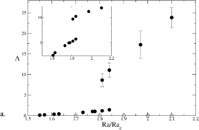
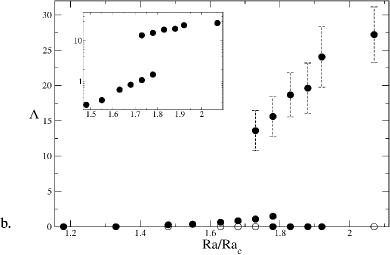
Figure 1: Weak- and strong-field branches for ${\rm E}=3\cdot 10^{-4}$ and a: ${\rm Pm}=14$, and b: ${\rm Pm}=18$. Symbol indicate the time averaged Elsasser number ($\bullet$ stable, $\circ$ unstable), time variability of the dynamo mode is reported using the standard deviation (indicated with error bars). The Insets present the same graphs in lin-log scale, so that the weak-branch is more clearly visible.

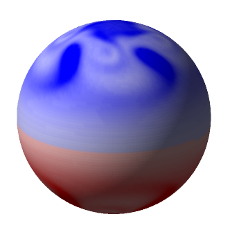
a.       b.

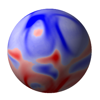
Figure 2: Radial component of the magnetic field produced at the surface of the model for ${\rm Pm}=18$, and ${\rm Ra}/{\rm Ra}_{c}=1.73$ on the weak-field (a.) and strong-field (b.) branches. The field is characterised by a strong axial dipolar component on both branches.

Following the same approach as Morin & Dormy (2009), we study the bifurcation from the purely hydrodynamic solution to the dynamo state using the Rayleigh number as control parameter. At fixed E and Pm, the Rayleigh number needs to exceed a given value for a dynamo solution (non-vanishing field) to exist. We report here direct numerical simulations performed at large values of the magnetic Prandtl number Pm. One may object that such parameter regime is irrelevant to dynamo action in liquid metals (characterised by a small magnetic Prandtl number). We will however argue that considering large values of Pm can compensate for the excessive role of inertial terms in numerical dynamo models, and is a necessary consequence of the large values assumed by the Ekman number.

Figure 1 presents the bifurcation diagrams obtained for ${\rm Pm}={\rm q}=14$ and ${\rm Pm}={\rm q}=18$. The magnetic field strength, as measured by the classical Elsasser number ${\mbox{$\Lambda$}}={B^{2}}/(2\,\Omega\,\rho\,\mu\,\eta)$ is represented versus the Rayleigh number, normalised by its value at the onset of thermal convection ${\rm Ra}_{c}$ (here ${\rm Ra}_{c}=60.8$). Each point on this figure corresponds to a time averaged fully three-dimensional simulation. The time variability of the dynamo mode is reported using the standard deviation.

Figure 1 is characterised by a supercritical bifurcation (as reported in Morin & Dormy (2009) for their “large” values of the magnetic Prandtl number, i.e. ${\rm Pm}=6$). However this first dynamo branch rapidly destabilises to a second branch of much stronger amplitude. This strong-field branch can be maintained for decreasing values of the Rayleigh number. The magnetic field is dominated by the axial dipole on both branches (see Figure  2). The strong-field branch on Fig 1a is hysteretic to the onset of dynamo itself: once on this branch, the control parameter can be decreased below the critical value for dynamo bifurcation, while maintaining a dipolar magnetic field.

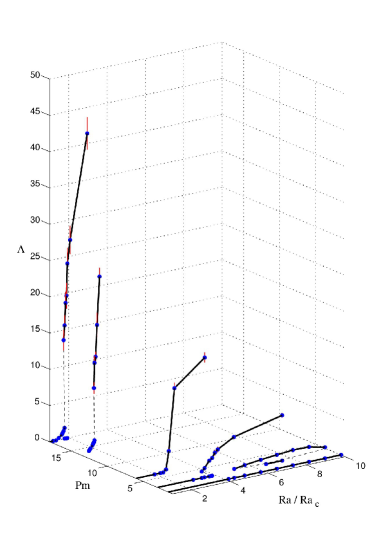
Figure 3: Three-dimensional bifurcation diagram for a fixed Ekman number ${\rm E}=3\cdot 10^{-4}$. Solid lines mark linear interpolation between realised direct numerical simulations. Dashed lines offer a plausible interpretation of the unstable branches.

This new branch completes the sequence of bifurcation diagrams introduced in Morin & Dormy (2009), and the complete three dimensional bifurcation diagram (including the results of Morin & Dormy, 2009) for ${\rm E}=3\,10^{-4}$ and ${\rm Pr}=1$ is reported on Figure 3 versus ${\rm Ra}/{\rm Ra}_{c}$ and ${\rm Pm}$. The corresponding two-dimensional bifurcation diagrams, for lower values of Pm, are available in Morin & Dormy (2009). On such a three-dimensional diagram, the dynamo bifurcation can also be envisaged at fixed value of ${\rm Ra}/{\rm Ra}_{c}$ and varying ${\rm Pm}$.

Figure 3 demonstrates how the transition between the different types of bifurcation takes place for different values of Pm. The study of Morin & Dormy (2009) indicates that as E is decreased (in the moderate range numerically achievable), the overall bifurcation diagram remains largely unaltered but shifted towards lower values of Pm and larger ${\rm Ra}/{\rm Ra}_{c}$.

Transitions between these two branches of dynamo solutions are obtained by varying only slightly the control parameter at the edge of a given branch. This can produce either a runaway field growth (Fig 4a), or a catastrophic collapse (Fig 4b) of the magnetic field. The time at which the forcing (as measured by the Rayleigh number) has been modified (by less than $3\%$ in each case) is indicated by an arrow on each graph.

No significant changes on the typical length scale of the flow can be reported by comparing the weak- and strong-field branches. This is probably due to the fact that the viscous length scale is not very small at the value of the Ekman number considered here ($3\cdot 10^{-4}$). Smaller values of the Ekman number are undoubtedly needed if one is to appreciate a change in the typical length scale of the flow. One can note however that the Nusselt number is $80\%$ larger on the strong-field branch than on the weak-field branch.

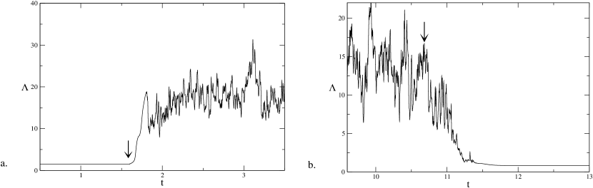
Figure 4: Transition between the weak- and strong-field branches for ${\rm E}=3\cdot 10^{-4}$ and ${\rm Pm}=18$ (same as figure 1.b). Runaway growth from the weak- to the strong-field branch as ${\rm Ra}/{\rm Ra}_{c}$ is increased (arrow) from $1.78$ to $1.83$ (a) and catastrophic decay to the weak-field branch as it is decreased (arrow) from $1.73$ to $1.68$ (b). The lower branch (left part of (a) and right part of (b) corresponds to small, but non-vanishing magnetic fields.

4 Force balance

The bifurcation diagram presented on Figure 1 is reminiscent of a longstanding theoretical expectation originally introduced as the ‘weak’- and ‘strong’-field branch (see Roberts, 1978; Roberts & Soward, 1992). The existence of these two branches in the limit of vanishing viscous forces was introduced through the investigation of magneto-convection studies (see Proctor, 1994; Fearn et al, 1986, for reviews).

Soward (1979) investigated the onset of magneto-convection in the cylindrical annulus configuration with sloping boundaries. He found that in most cases the critical Rayleigh number first starts to increase with the Elsasser number, until ${\mbox{$\Lambda$}}\sim{\cal O}({\rm E}^{1/3})$, before decreasing. This pointed to the probable existence of a weak-field branch, and the occurrence of a turning point marking the end of the weak-field branch when ${\mbox{$\Lambda$}}\sim{\cal O}({\rm E}^{1/3})$. Simultaneously, Fearn (1979a, b) performed a similar study in the spherical geometry. There again, the Rayleigh number for the thermal Rossby mode may first increase with increasing Elsasser number, yet it eventually decreases to reach a minimum for ${\mbox{$\Lambda$}}\sim{\cal O}(1)$. A more recent study of magneto-convection (Jones et al, 2003) focused on the “weak-field” regime and confirmed its existence.

The above asymptotic scenario assumes a small value of both E and Pm, whereas direct numerical simulations in the self-excited dynamo regime require overestimated values of both numbers.

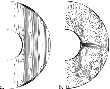
Figure 5: Azimuthal velocity in a meridional cross-section for an arbitrary time on the weak-field branch (a.) and on the strong-field branch (b.) for the same parameter set (${\rm Pm}=18$, ${\rm Ra}/{\rm Ra}_{c}=1.73$).

In order to test the above ideas in the numerical simulations, we need to investigate the dominant force balance relevant to these dynamo modes. Figure 5 presents an instantaneous cross-section of the zonal velocity on both branches for a given parameter set (${\rm Pm}=18$, ${\rm Ra}/{\rm Ra}_{c}=1.73$). The contour intervals are equally spaced between the minimum and the maximum value for each figure. The zonal flow is nearly three times larger on the left panel, so that the contour intervals are not identical on the two plots. On the one hand, the weak-field branch saturates while the zonal flow remains essentially geostrophic; the flow is characterised by quasi-geostrophic convection columns. The zonal flow on the strong-field branch, on the other hand, strongly departs from bidimensionality, demonstrating that the rapid rotation constraint has been relaxed. On figure 5.b, a localised jet appears near the equator which marks a clear departure from geostrophy. The flow is in general less anisotropic along the direction of the axis of rotation. If this corresponds to the weak-field vs strong-field branches as introduced by P.H. Roberts, it implies that the Lorentz forced has achieved a balance with the Coriolis term and thus relaxed the rapid rotation constraint. This dominant balance is usually referred to as the “magnetostrophic balance”.

The Elsasser number $\Lambda$ was introduced to measure an order-of-magnitude of the relative strength of the Lorentz force with respect to the Coriolis force. It achieves this aim remarkably well in asymptotic studies, for the huge distinction between the strong-field balance, characterised by ${\mbox{$\Lambda$}}\sim{\cal O}(1)$ and the weak-field branch characterised by ${\mbox{$\Lambda$}}\sim{\cal O}({\rm E}^{1/3})$. In numerical works, however, as small parameters (such as the Ekman number) are not asymptotically small, the measure provided by this non-dimensional number is then not accurate enough. Finer estimates of this force balance can then be constructed. Introducing $\left\{\cdot\right\}$ as an “order of magnitude” operator, we can write

$$\frac{\left\{(\mu\rho)^{-1}\left(\mbox{\boldmath$\nabla$}\times\mbox{\bf B}\right)\times\mbox{\bf B}\right\}}{\left\{2\,\Omega\times\mbox{\bf u}\right\}}=\frac{B^{2}}{2\,\Omega\,\mu\,\rho\,U\,\ell_{B}}\,,$$ (4)

where $U$ is a typical, say root mean square (r.m.s.) value for the velocity field, $B$ a typical value for the magnetic field, and $\ell_{B}$ the typical magnetic dissipation length scale (see also Oruba & Dormy, 2014a).

The classical definition of the Elsasser number is obtained by assuming $\ell_{B}\sim L$ and a statistical balance between induction and diffusion of the magnetic field

$$\left\{\mbox{\boldmath$\nabla$}\times\left(\mbox{\bf u}\times\mbox{\bf B}\right)\right\}\sim\left\{\eta\mbox{\boldmath$\nabla$}\times\mbox{\boldmath$\nabla$}\times\mbox{\bf B}\right\}\,,$$ (5)

which yields $U\sim\eta/L$. Then (4) provides the standard expression for the Elsasser number ${\mbox{$\Lambda$}}={B^{2}}/(2\,\Omega\,\rho\,\mu\,\eta)\,.$ This expression provides a sensible description of the force balance for asymptotic studies, yet finer estimates appear to be needed for numerical studies.

One can note, for example that $U\sim\eta/L$ amounts to assuming Rm$\sim{\cal O}(1)$. A finer description of the force balance (4) can be obtained by estimating $U$ via ${\rm Rm}\,\eta/L$. Inserting this definition in (4) yields

$${\mbox{$\Lambda^{\prime}$}}=\frac{B^{2}\,L}{2\,\Omega\,\rho\,\mu\,\eta\,{\rm Rm}\,\ell_{B}}={\mbox{$\Lambda$}}\,\frac{L}{{\rm Rm}\,\ell_{B}}\,.$$ (6)

Table 1 presents a comparison of the classical Elsasser number $\Lambda$ and the modified Elsasser number $\Lambda^{\prime}$ on both branches. The magnetic Reynolds number Rm is here defined on the RMS velocity, and the typical magnetic dissipation length scale $\ell_{B}$ is defined, as in Oruba & Dormy (2014a), as

$$\ell_{B}^{2}=\frac{\int_{V}\mbox{\bf B}^{2}{\rm d}V}{\int_{V}(\mbox{\boldmath$\nabla$}\times\mbox{\bf B})^{2}{\rm d}V}\,.$$ (7)

Figure 6 presents the time variation of the modified Elsasser number on the weak-field branch (dashed) and on the strong-field branch (solid line) for the same parameter set, ${\rm Pm}=18$, ${\rm Ra}/{\rm Ra}_{c}=1.73$.

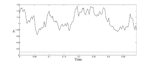
Figure 6: Fluctuation of the modified Elsasser number on both branches for the same parameter set (${\rm Pm}=18$, ${\rm Ra}/{\rm Ra}_{c}=1.73$).

The modified Elsasser number, offering a finer description of the force balance, reveals that the Lorentz force is significantly weaker than the Coriolis force on the weak-field branch and that the two terms are indeed of comparable amplitude on the strong-field branch.

Branch	${\rm Ra}$	${\rm Ra}/{\rm Ra}_{c}$	${\rm Pm}$	Rm	$\ell_{B}$	$\Lambda$	$\Lambda^{\prime}$
Weak	105	1.73	18	195	0.097	1.14	0.06
Strong	105	1.73	18	145	0.082	13.6	1.14
Strong	125	2.05	18	207	0.075	27.2	1.75
Strong	112	1.84	14	150	0.083	11.05	0.89

Table 1: Typical estimates of the Elsasser number and the modified Elsasser number (${\mbox{$\Lambda^{\prime}$}}={\mbox{$\Lambda$}}\,L/({\rm Rm}\,\ell_{B})$, see text) on the weak- and strong-field branches. The modified Elsasser number offers a finer measurement of the force balance.

The orders of magnitude derived above indicate that the anticipated balance between the Coriolis and Lorentz forces is plausible. To achieve a finer validation, than simple orders of magnitude, we can assess whether the two terms tend to balance each other locally in space. To this aim, one can consider the curl of the momentum equation (1), neglecting both the inertial term and the viscous term,

$${-}2\,\frac{\partial\mbox{\bf u}}{\partial z}\sim{\rm Ra}{\rm q}\,\mbox{\boldmath$\nabla$}\times(T\mbox{\bf r})+\mbox{\boldmath$\nabla$}\times\left(\left(\mbox{\boldmath$\nabla$}\times\mbox{\bf B}\right)\times\mbox{\bf B}\right)\,.$$ (8)

If we now consider the radial component of the above equation, i.e. its toroidal component, the first term on the right-hand-side disappears. The remaining two terms were computed numerically at a given instant in time and on a cross-section in an arbitrary meridional plane. These quantities are presented on Figure 7.

Deviations between the two cross-sections can imply only non-vanishing inertial and/or viscous effects. Estimations of these terms reveals that the viscous term accounts for the differences visible on the figures (inertia being one order of magnitude smaller). The comparison reveals such effects (in particular in viscous boundary layers), but otherwise clearly demonstrates that the radial component of the curl of the Lorentz force balances that of the Coriolis force, as expected in the strong-field limit.

The Viscous force will of course not always be negligible in the parameter regime considered here. It can be more important at some places or time. To illustrate this, the quantities represented on Figure 7 are represented at a later time in the form of three-dimensional isosurfaces on Figure 8. The blue and red isosurfaces respectively, correspond to $\pm 90\%$ of the peak values. While deviations from magnetostrophy are obvious in particular comparing the centre of each figure, the dominant magnetostrophic balance is highlighted. Deviations are here primarily due to viscous forces. Boundary layers have not been represented in these figures.

Figures 7 and 8 highlight the balance between the non-gradient part of the Lorentz and Coriolis terms. Differences are primarily due to viscous effects and remain small (but non-vanishing) on average. The r.m.s value of the sum of the two quantities plotted in these figures, averaged in time, exceeds by a factor 5 that of their difference.

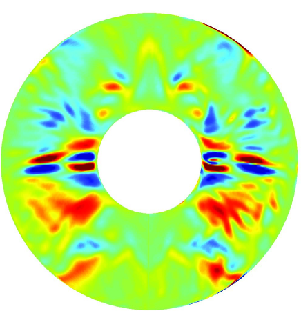
Figure 7: Meridional cross-sections on the strong-field branch at a given time for the same parameters and same phase as in figure 5.b. On the left side $-2\,{\partial\mbox{\bf u}}/{\partial z}\cdot\mbox{\bf e}_{r}$ is presented, and on the right side $\left(\mbox{\boldmath$\nabla$}\times\left(\left(\mbox{\boldmath$\nabla$}\times\mbox{\bf B}\right)\times\mbox{\bf B}\right)\right)\cdot\mbox{\bf e}_{r}$ using the same color range.

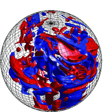
a.       b.

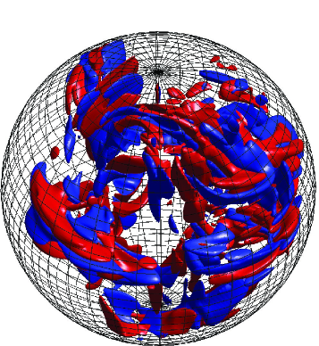
Figure 8: Three dimensional iso-surfaces of the radial component of the curl of the Coriolis force (a.) and the Lorentz force (b.).

5 Discussion

Numerical models of self-excited dynamos usually correspond to two distinct branches, either viscous-dipolar or inertial-multipolar (e.g. Kutzner & Christensen, 2002; Jones, 2011; Oruba & Dormy, 2014b). This work introduces a third dynamo branch in the parameter regime which is numerically achievable with present computational resources. What if this new branch was relevant to the geodynamo?

5.1 Physical interpretation

In numerical models, at moderate Ekman numbers, inertial forces increase too rapidly with the control parameter (the Rayleigh number) to allow for a strong-field branch balance (the magnetic field amplitude does not increase rapidly enough, and inertial forces enter the dominant balance before the Lorentz force). In order to observe at a given Ekman number the third branch introduced in this work, one needs to increase the magnetic Prandtl number in order to decrease the prefactor of inertial forces. This results in a larger magnetic Reynolds number for a given value of the Rayleigh number.

Using large values of the magnetic Prandtl number thus allows for the runaway field solution anticipated theoretically. We observe that the Lorentz force becomes large enough (while inertia remains small enough not to modify the nature of dynamo action) in order for the Lorentz force to relax the constraints of rapid rotation.

Figure 9: Sketch of a tentative two dimensional bifurcation diagram near the region of existence of the weak- and strong-field branches. The fold in the surface accounts for the observed two branches of solutions.

The three-dimensional bifurcation diagram (Figure 3) can be tentatively sketched near the region in which the strong- and weak-field branches coexist (see Figure 9). The change of branch as Ra is varied at fixed Pm corresponds to a fold of the surface of solutions. It is clear from such a representation that, in the two dimensional parameter space (E, Pm), one can continuously move from the lower to the upper branch, avoiding the fold singularity. The corresponding intermediate models would presumably involve a continuous decrease of viscous forces. These intermediate solutions (at lower values of Pm) will then have characteristics continuously varying from that of the weak-branch to that of the strong-branch. It follows that some numerical models obtained at lower values of Pm will necessarily have some characteristics of the strong-field branch. Such is the case in particular for models with a large magnetic Prandtl number (though not large enough for the bistability to occur) and large Rayleigh number (so that viscous effects are reduced), but not too large (to avoid the inertial, non-dipolar, branch). In such a model, time-averaged force balance can tend to magnetostrophy (e.g. Aubert, 2005; Sreenivasan et al, 2014).

It should be stressed as well that large values of Pm have been studied in a few earlier numerical works (e.g. Olson et al, 2011; Gubbins et al, 2007), though without pointing to the existence of a weak- and a strong-field branch.

5.2 Distinguished limit

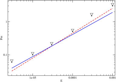
Figure 10: Minimal value of the magnetic Prandtl number ${\rm Pm}_{c}$ below which the dipolar viscous branch is lost for a given Ekman number. Triangles correspond to numerical data produced by Christensen & Aubert (2006), and the dashed line to their empirical fit ${\rm Pm}_{c}\sim{\rm E}^{3/4}$. The solid line corresponds to the ${\rm Pm_{c}}\sim{\rm E}^{2/3}$ scaling (Dormy & Le Mouël, 2010).

We have seen in Morin & Dormy (2009) that the nature of the dynamo bifurcation strongly depends on the parameters (in particular ${\rm Pm}$ at fixed ${\rm E}$). The current approach to geodynamo modelling consists either in trying to explore the whole range of magnetic Prandtl number at fixed Ekman number, or, too often, in trying to decrease the value of the magnetic Prandtl number as low as possible for a given Ekman number (the viscous dipolar solution being lost for ${\rm Pm}$ lower than a critical value ${\rm Pm}_{c}$). The present work suggests that, in order to preserve the relevant force balance, both ${\rm E}$ and ${\rm Pm}$ being small parameters in the Earth’s core, they could be related in numerical studies via a distinguished limit, involving only one small parameter $\varepsilon$. Ideally the nature of the dynamo bifurcation should be preserved in the limiting process.

In order to propose such a scaling, one could be guided by the scaling for the minimum magnetic Prandtl number ${\rm Pm}_{c}$ as a function of the Ekman number ${\rm E}$. This relations stems from numerical simulations in the viscous branch: it is however the only regime that has been widely covered in numerical simulations. The available data are illustrated in Figure 10. Decreasing ${\rm Pm}$ at otherwise fixed parameters amounts to decreasing the magnetic Reynolds number. The dipolar viscous branch is thus lost for ${\rm Pm}<Pm_{c}$ which decreases with decreasing values of the Ekman number (Kutzner & Christensen, 2002; Christensen & Aubert, 2006). It follows a scaling of the form ${\rm Pm}_{c}\sim{\rm E}^{\alpha}\,,$ in which $\alpha$ needs to be determined. Christensen & Aubert (2006) proposed an empirical fit with $\alpha=3/4$. Dormy & Le Mouël (2010) proposed on the basis of exponential growth associated with a locally time dependent shear, a scaling of the form $\alpha=2/3$, which seems to match the numerical data equally well and is guided by a plausible argument. For simplicity, we will use this latter scaling for illustration purposes below, but the same reasoning would apply with a different exponent.

In order to introduce a single small parameter $\varepsilon$ to control both quantities, one can write ${\rm E}\sim A\,\varepsilon^{B}$ and ${\rm Pm}\sim C\,\varepsilon^{D}\,.$ Without loss of generality, one can set $A=1$, up to a redefinition of $\varepsilon$. In order to preserve the nature of the dynamo bifurcation in the limiting process, we propose ${\rm Pm}^{3}\sim{\rm E}^{2}\,,$ and it follows that

$${\rm E}\sim\varepsilon^{3}\qquad{\rm Pm}\sim C\,\varepsilon^{2}\,.$$ (9)

This distinguished limit ensures that both ${\rm E}$ and ${\rm Pm}$ tend to zero with $\varepsilon$ and that they are related in such a way that the nature of the solution, i.e. its dynamo property, should be preserved in the limiting process. The coefficient $C$ can be estimated via sensible estimates for the Earth’s core, such as ${\rm E}\simeq 10^{-14}$ and ${\rm Pm}\simeq 10^{-6}$: the first equation naturally provides $\varepsilon\simeq 2\cdot 10^{-5}$, while the second yields $C\simeq 2\cdot 10^{3}$, which is a rather large prefactor. Applying (9) to the numerical models presented in this work (with ${\rm E}=3\cdot 10^{-4}$), in turn yields ${\rm Pm}\simeq 10$. This distinguished limit thus yields values of the magnetic Prandtl number larger than unity (similar to those used in our numerical studies) for the Ekman number investigated here.

The idea behind such distinguished limits is not to aim at a large magnetic Prandtl number limit, as both the Ekman number and the Prandtl number vanish asymptotically in the limiting process. For the moderate values of the small parameter $\varepsilon$, achievable with current computational resources, the proposed distinguished limit however suggests that the use of values of ${\rm Pm}$ larger than unity is relevant.

As computational resources increase, one should be able in the near future to investigate the behaviour of this strong-field branch for lower values of the Ekman number, and thus lower values of the magnetic Prandtl number. This will allow investigation of interesting and important issues in particular on the evolution of the relevant length scale as the magnetic Prandtl number becomes less than unity.

6 Conclusions

A dominant magnetostrophic balance can be established in direct numerical simulations of rotating spherical dynamos. Magnetostrophy is not satisfied everywhere and for for all time.

The weak- and strong-field branches anticipated from asymptotic studies of magneto-convection are approached in direct numerical simulations for some parameter values. In order for inertial forces to be small enough to allow this regime, it is necessary to relate the magnetic Prandtl number to the Ekman number in the form of a distinguished limit. Further studies will need to decrease the Ekman number to ensure a clear distinction between the small scale flow on the viscous branch and the large-scale flow on the strong-field branch. The next important challenge for direct numerical models would be to maintain dynamo action for ${\rm Ra}/{\rm Ra}_{c}<1$ as expected theoretically. The role of the Prandtl number (fixed to unity here) in controlling the relative strength of the advection versus diffusion of heat also deserves further studies. Further numerical studies of this branch could include varying Pr. For instance the limit of large Pm with small q would allow for significant nonlinearities in the energy equation, while controlling the amplitude of inertial effects.